Variations on the Vev Flip-Flop:
Instantaneous Freeze-out and Decaying Dark Matter

Abstract

In this work we consider a simple model for dark matter and identify regions of parameter space where the relic abundance is set via kinematic thresholds, which open and close due to thermal effects. We discuss instantaneous freeze-out, where dark matter suddenly freezes-out when the channel connecting dark matter to the thermal bath closes, and decaying dark matter, where dark matter freezes-out while relativistic and later decays when a kinematic threshold temporarily opens. These mechanisms can occur in the vicinity of a one-step or a two-step phase transition. In all cases thermal effects provide this dynamic behaviour, while ensuring that dark matter remains stable until the present day.

I Introduction

Understanding the nature of dark matter (DM) is one of the most pressing and elusive problems in physics. For a long time, the best-motivated candidate has been the Weakly Interacting Massive Particle (WIMP). In this picture, DM particles are hypothesised to be heavy ($m_{\text{DM}}\gtrsim 100$ GeV) and to have weak but non-negligible interactions with Standard Model (SM) particles. In the very early universe, these interactions keep the DM and the SM particles in thermal and chemical equilibrium, until eventually the expansion of the universe dilutes the DM density to the extent that DM annihilation into SM particles ceases, and a relic abundance survives to the present day (a process known as freeze-out). However, in spite of a vigorous, multi-pronged search programme [1, 2, 3, 4, 5, 6], there is still no evidence for WIMPs, and the remaining allowed parameter space has been drastically reduced.

There is currently a large effort studying alternative mechanisms of DM production [7]. In the early universe, the SM particles formed a hot, thermal bath and the effects of this plasma can have a dramatic impact on particle properties and interactions. These finite-temperature effects are known to cause important phenomena in the development of the universe, such as the electroweak phase transition (EWPT). Recently there has been interest in understanding the impact of finite temperature effects in mechanisms of DM production [8, 9, 10, 11, 12, 13, 14, 15, 16, 17].

In the present work we examine the mechanism presented in [12, 15] where the DM abundance is set not via freeze-out but via a period of DM decay, which occurs when a new scalar field temporarily obtains a vacuum expectation value (vev) just before the EWPT. We find that the key feature required for this period of decay is the opening and closing of kinematic thresholds, due to particle masses obtaining temperature dependent corrections. In the early universe, bosons receive large finite temperature corrections and their masses and vevs should be treated as functions of temperature. In section II, we propose a simple model which retains the key features of the mechanism in [12]. With this simple model, we identify further regions of parameter space where interesting DM production mechanisms can appear. We first discuss the effective potential at finite temperatures in section III, the thermal bath in section IV and Boltzmann equations to track the DM abundance in section V. With this framework, we describe instantaneous freeze-out in section VI, where DM freezes-out abruptly when a kinematic channel closes. In section VII we show that a period of DM decay can set the relic abundance, dubbed decaying dark matter, when a new scalar field obtains a vev in a one-step phase transition, while in section VIII we look at a situation similar to that described in [12] where a two-step phase transition (or a vev flip-flop) can lead to a period of decaying dark matter. Finally, in section IX we briefly consider the experimental constraints on the different scenarios.

II The Model

Field	Spin	$\mathbb{Z}_{2}$	mass scale (at $T=0$)
$S$	0	$+1$	$\sim 0.1\text{ -- }100\,\text{GeV}$
$\chi$	$\frac{1}{2}$	$-1$	$\sim 5\,\text{GeV}\text{ -- }5\,\text{TeV}$
$\psi$	$\frac{1}{2}$	$-1$	$\sim 5\,\text{GeV}\text{ -- }5\,\text{TeV}$

Table 1: The new particles we introduce in section II with their respective charges and mass scales. All new particles are SM gauge singlets.

To demonstrate the effects as clearly as possible, we consider a simple model consisting of the SM plus a real scalar, $S$, and two dark sector Dirac fermions, $\chi$ and $\psi$, shown in table 1. In what follows, $\chi$ will constitute the dominant component of dark matter. These particles will all be gauge singlets, and will have masses in the GeV to TeV range.

The Lagrangian for these fields is

$$\mathcal{L} \supset\frac{1}{2}(\partial_{\mu}S)(\partial^{\mu}S)+\bar{\psi}(i\not{\partial}-\tilde{m}_{\psi})\psi+\bar{\chi}(i\not{\partial}-m_{\chi})\chi$$

$$\qquad-\big{[}y_{\chi\psi}\,\bar{\psi}S\chi+h.c.\big{]}-y_{\chi}\,\bar{\chi}S\chi-y_{\psi}\,\bar{\psi}S\psi-V(H,S)\,,$$ (1)

with

$$V(H,S) =-\mu_{H}^{2}H^{\dagger}H+\lambda_{H}\,(H^{\dagger}H)^{2}-\frac{1}{2}\mu_{S}^{2}S^{2}+\frac{\lambda_{S}}{4!}S^{4}+\frac{\lambda_{p}}{2}\,S^{2}(H^{\dagger}H)\,.$$ (2)

In our notation, the SM Higgs potential has $\mu_{H}\simeq 88\,\text{GeV}$ and $\lambda_{H}\simeq 0.12$, with $H=(G^{+},(h+iG^{0})/\sqrt{2})$. We choose a basis where the CP-even, neutral component $h$ obtains the vev. We see in eq. 2 that the only interaction at dimension-4 between these new particles and the Standard Model is the Higgs portal term $(\lambda_{p}/2)\,S^{2}(H^{\dagger}H)$. Although in principle there may also be the terms $S^{3}$ and $S(H^{\dagger}H)$, we assume these couplings to be negligibly small. In sections VI and VII we will consider $\lambda_{p}\ll 1$. In this regime the scalar fields decouple and we can consider the evolution of $S$ alone, simplifying the picture. In section VIII we will consider $\lambda_{p}\simeq 1$. For the new Yukawa couplings we will typically consider $y_{\psi}\simeq 1$, $y_{\chi\psi}\sim 10^{-7}$ and $y_{\chi}\simeq 0$. A large $y_{\psi}$ means that $\psi$ will remain in thermal equilibrium throughout the processes affecting the $\chi$ abundance. This small $y_{\chi\psi}$ will however make direct and indirect detection of dark matter challenging. Within this model, none of the operators with small couplings will be generated at a significant level via loops.

We will focus on the regions of parameter space where finite temperature effects from the scalar sector have a significant impact on the final abundance of $\chi$. We know from the standard WIMP picture that the observed relic abundance is obtained if DM freezes-out when its mass is 20 – 30 times greater than the freeze-out temperature. Since we do not have abundances below the equilibrium abundance, this provides a lower limit on $m_{\chi}$. If the DM mass is much greater than the temperature at which the abundance is set, then finite temperature effects will be small compared to zero temperature effects. This tension means that for the mechanisms presented in this paper, we will generally focus on the parameter space where $m_{\chi},\tilde{m}_{\psi}\simeq 30\,\mu_{S}$. We choose the signs of the Yukawas so that for positive couplings, $\left\langle S\right\rangle\neq 0$ will give a positive contribution to the mass. In table 2 we summarise the different mechanisms and highlight the relevant parameter space.

Finally we emphasise that many models can accommodate degenerate or nearly-degenerate vector-like fermions, while the hierarchy between the masses of the new fermions and the new scalar may be expected since their mass scales are not directly connected. Similarly, while the strong hierarchy of the new Yukawa couplings $y_{\psi}$, $y_{\chi\psi}$ and $y_{\chi}$ is not explained, its origin could be related to the SM flavour puzzle. Although we focus on this particular region of parameter space to highlight the importance of finite temperature effects, which will prove to dramatically alter the DM relic abundance, we note that these effects may still be numerically important in much wider regions of parameter space.

P.T.	Mechanism	$\lambda_{p}$	$y_{\psi}$	$m_{S}(T=0)$	$y_{\chi\psi}$	$\chi$ decay ended by	Section
One–step	Instantaneous f.o.	$\ll 1$	$>0$	$0.1\text{ -- }10\,\text{GeV}$	$\sim 10^{-7}$	$\left\langle S\right\rangle$	VI
One–step	Decaying DM	$\ll 1$	$>0$	$0.1\text{ -- }10\,\text{GeV}$	$\sim 10^{-8}$	$\left\langle S\right\rangle$	VII
Two–step	Instantaneous f.o.	$\sim 1$	$<0$	$\sim 100\,\text{GeV}$	$\sim 10^{-6}$	vev flip-flop	VIII
Two–step	Decaying DM	$\sim 1$	$<0$	$\sim 100\,\text{GeV}$	$\sim 10^{-7}$	vev flip-flop	VIII

Table 2: A summary of the mechanisms that operate in various regions of parameter space. In the first column we give the nature of the phase transition of the new scalar $S$. In the penultimate column we note whether the $\chi$ decay and inverse–decay channel closes due to the vev of $S$ becoming sufficiently large, or to the vev of $S$ becoming zero after a ‘vev flip-flop’.

III The Effective Potential at Finite Temperatures

We first turn to the effective potential of the scalar fields, and describe the finite temperature corrections we include. The effective potential is analogous to the free-energy of a system, and the system (in this case the vacuum scalar field configuration) will move to the minimum of the effective potential. The leading terms in the zero-temperature effective potential are the tree-level potential $V^{\text{tree}}(h,S)$, the one-loop Coleman-Weinberg correction $V^{\text{CW}}(h,S)$ [18], and a one-loop counterterm $V^{\text{CT}}(h,S)$. The leading corrections at finite temperature are the one-loop thermal corrections $V^{T}(h,S,T)$ [19] and the resummed higher order “daisy” diagrams [20, 21, 22]. The one-loop effective potential at finite temperature, $V^{\text{eff}}(h,S,T)$, is then

$$V^{\text{eff}}(h,S,T) =V^{\text{tree}}(h,S)+V^{\text{CW}}(h,S)+V^{\text{CT}}(h,S)+V^{T}(h,S,T)+V^{\text{daisy}}(h,S,T)\,.$$ (3)

The tree level potential $V^{\text{tree}}$ is given in eq. 2. The $T$-independent Coleman-Weinberg contribution is [18, 21]

$$V^{\text{CW}}(h,S) =\sum_{i}\frac{n_{i}}{64\pi^{2}}m_{i}^{4}(h,S)\bigg{[}\log\bigg{(}\frac{m_{i}^{2}(h,S)}{\Lambda^{2}}\bigg{)}-C_{i}\bigg{]}+V^{\text{CT}}(h,S)\,,$$ (4)

where the sum is over the eigenvalues of the field-dependent mass matrices of all fields which couple significantly to the scalars and $|n_{i}|$ accounts for their respective numbers of degrees of freedom. In our case $n_{h}=n_{G^{0}}=n_{S}=1$, $n_{G^{+}}=2$, $n_{Z}=3$, $n_{W}=6$ and $n_{t}=-12$. We do not include the lighter quarks as they couple only very weakly to the SM Higgs. The coefficient $n_{i}$ is positive for bosons and negative for fermions, due to their different statistics. As a renormalisation scale $\Lambda$ we use the characteristic scale of the $S$ field, $\mu_{S}$. Using the dimensional regularisation scheme, $C_{i}=5/6$ for gauge bosons and $C_{i}=3/2$ for scalars and fermions. The field-dependent masses of the CP even neutral scalars, in the basis $(h,s)$, are

$$m_{hS}^{2}= \,\begin{pmatrix}-\mu_{H}^{2}+3\,\lambda_{H}\,h^{2}+\frac{1}{2}\lambda_{p}\,S^{2}&\lambda_{p}\,h\,S\\ \lambda_{p}\,h\,S&-\mu_{S}^{2}+\frac{1}{2}\lambda_{S}\,S^{2}+\frac{1}{2}\lambda_{p}\,h^{2}\end{pmatrix},$$ (5)

while the field dependent masses of the remaining bosons are

$$m_{G}^{2} =-\mu_{H}^{2}+\lambda_{H}\,h^{2}+\frac{\lambda_{p}\,S^{2}}{2}\,,$$ (6)

$$m_{W^{\pm}}^{2} =\frac{1}{4}g^{2}\,h^{2}\,,$$ (7)

$$m_{Z}^{2} =\frac{1}{4}(g^{2}+g^{\prime 2})\,h^{2}\,,$$ (8)

$$m_{\gamma}^{2} =0\,,$$ (9)

$$m_{t}^{2} =\frac{1}{2}y_{t}^{2}\,h^{2}\,,$$ (10)

where $g^{\prime}$ and $g$ are the SM $u(1)_{Y}$ and $su(2)_{L}$ coupling constants, respectively. Although the dark sector fermion $\psi$ couples strongly to $S$, we neglect its contribution since its mass is always much larger than either the temperatures or the scalar field values we consider [23].

To ensure that $\langle H\rangle=\mu_{H}/\sqrt{\lambda_{H}}$, $m_{h}^{2}=2\mu_{H}^{2}$ and that $m_{S}$ is given by its tree level value at $T=0$, we add the counterterm

$$V^{\text{CT}}(h,S) =-\frac{1}{2}\delta_{\mu}h^{2}+\frac{1}{4}\delta_{\lambda}h^{4}-\frac{1}{2}\delta_{\mu_{S}}S^{2},$$ (11)

where the factors $\delta_{i}$ are

$$\delta_{\mu} =\frac{3}{2v}\left.\frac{\partial V^{\text{CW}}}{\partial h}\right|_{v}-\frac{1}{2}\left.\frac{\partial^{2}V^{\text{CW}}}{\partial h^{2}}\right|_{v}\,,$$ (12)

$$\delta_{\lambda} =\frac{1}{2v^{3}}\bigg{(}\left.\frac{\partial V^{\text{CW}}}{\partial h}\right|_{v}-v\left.\frac{\partial^{2}V^{\text{CW}}}{\partial h^{2}}\right|_{v}\bigg{)}\,,$$ (13)

$$\delta_{\mu_{S}} =\left.\frac{\partial^{2}V^{\text{CW}}}{\partial S^{2}}\right|_{v}\,.$$ (14)

The one-loop finite temperature correction is [19]

$$V^{T}(h,S,T) =\sum_{i}\frac{n_{i}T^{4}}{2\pi^{2}}\int_{0}^{\infty}\!dx\,x^{2}\log\bigg{[}1\pm\exp\Big{(}-\sqrt{x^{2}+m_{i}^{2}(h,S)/T^{2}}\Big{)}\bigg{]}\,,$$ (15)

where again we sum over the same eigenvalues as in eq. 4. The positive sign in the integrand is for fermions and the negative sign is for bosons.

Finally, higher order diagrams containing the bosons give rise to the so-called “daisy” corrections [20, 21, 24, 22]

$$V^{\text{daisy}}(h,S,T) =-\frac{T}{12\pi}\sum_{i}n_{i}\Big{(}\left[m^{2}(h,S)+\Pi(T)\right]_{i}^{\frac{3}{2}}-\left[m^{2}(h,S)\right]_{i}^{\frac{3}{2}}\Big{)}\,,$$ (16)

where the first term should be interpreted as the $i$-th eigenvalue of the matrix-valued quantity $[m^{2}(h,S)+\Pi(T)]^{3/2}$. Here, $m^{2}(h,S)$ is the block-diagonal matrix composed of the individual mass matrices [25]. This sum runs only over the bosonic degrees of freedom. The thermal (Debye) masses [20] in eq. 16 are

$$\Pi_{h,G^{0},G^{+}} =\tfrac{1}{48}T^{2}\left(9g^{2}+3g^{\prime 2}+24\lambda_{H}+12y_{t}^{2}+2\lambda_{p}\right)\,,$$ (17)

$$\Pi_{S} =\tfrac{1}{24}T^{2}\left(4\lambda_{p}+\lambda_{S}\right)\,,$$ (18)

$$\Pi_{W^{1,2,3}}^{L} =\tfrac{11}{6}g^{2}T^{2}\,,$$ (19)

$$\Pi_{W^{1,2,3}}^{T} =0\,,$$ (20)

$$\Pi_{B}^{L} =\tfrac{11}{6}g^{\prime 2}T^{2}\,,$$ (21)

$$\Pi_{B}^{T} =0\,,$$ (22)

where $\Pi_{h,G^{0},G^{+}}$ are the thermal masses of the components of $H$, $\Pi_{S}$ is the thermal mass of the components of $S$ and $\Pi_{W,B}$ are the thermal masses of the electroweak gauge boson. Only the longitudinal components of the gauge bosons obtain a non-zero thermal mass.

III.1 One-step Phase Transition

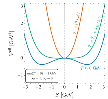
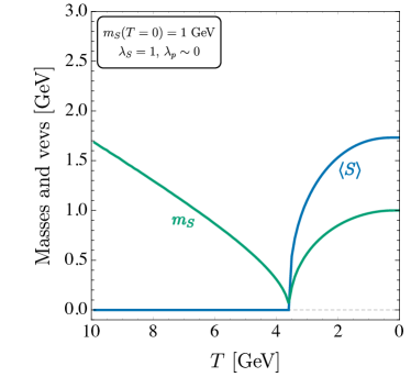
Figure 1: Left: the effective potential as a function of the $S$ field value at a high temperature ($10\,\text{GeV}$), at the critical temperature $T=T_{c}\approx 3.6\,\text{GeV}$ and at $T\approx 0\,\text{GeV}$. We subtract a constant term at each $T$ so that $V^{\text{eff}}(0)=0$. Right: the scalar mass and vev as a function of temperature.

With the effective potential in hand, we can now consider its behaviour in various regions of parameter space. We will first consider the regime where $\lambda_{p}\ll 1$, where the new scalar $S$ and the SM Higgs are weakly coupled. In this case the effective potential in $h$ and $S$ decouples, $V^{\text{eff}}(h,S,T)=V^{\text{eff}}(h,T)+V^{\text{eff}}(S,T)$. To consider the evolution of the new scalar, it is sufficient to consider the effective potential as a function of $S$ alone.

In fig. 1 (left) we show $V^{\text{eff}}(S,T)$ at several temperatures, for a particular choice of parameters. We will be interested in $\mu_{S}>0$, so that $S$ obtains a vev at $T=0$. We see that at high temperatures, thermal corrections dominate the effective potential and the minimum is at $S=0$, so there is no vev. As the universe expands, the temperature reduces until $T\simeq\mu_{S}$, at which point the finite $T$ corrections become similar in size to the $T=0$ potential. At $T_{c}$ there is a second-order phase transition and $S$ obtains a vev. As the universe cools further, the minima deepen and the vev increases to around $1.7\,\text{GeV}$.

As well as the position of the vev, the effective potential also determines the physical mass of the scalar $S$ in the thermal bath. Finite temperature corrections at one-loop are taken into account by taking the second derivative of the effective potential at a minimum. In fig. 1 (right) we show the evolution of the vev along with the physical $S$ mass, as a function of temperature. We see that the mass is large at high temperatures, becomes small through the phase transition (at $T_{c}$ the second derivative of the effective potential goes to zero), and reaches a value $\simeq\mu_{S}$ at zero temperature.

In sections VI and VII we will show that this temperature dependence of the mass and vev can lead to kinematic thresholds opening and closing, allowing dark matter to come into equilibrium or decay in some temperature window.

III.2 Two-step Phase Transition

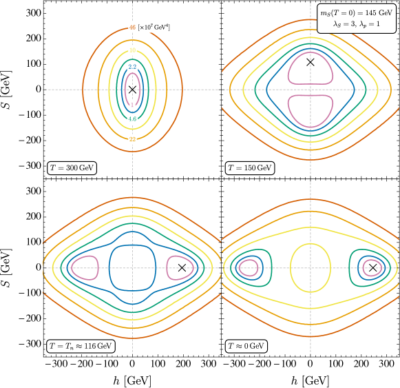
Figure 2: The effective potential $V^{\text{eff}}$ at $T=300\,\text{GeV}$ (top-left), at $T=150\,\text{GeV}$ (top-right), the nucleation temperature $T=T_{n}\approx 116\,\text{GeV}$ (bottom-left) and $T\approx 0\,\text{GeV}$ (bottom-right). In each plot we subtract a constant, the minimum value of the potential, to highlight the features around the minima. The black cross indicates the phase the Universe is in at the given temperatures.

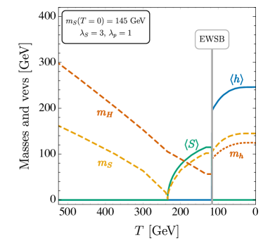
Figure 3: Evolution of the scalar vevs and masses with temperature for a particular parameter point. $m_{H}$ denotes the mass of the SM Higgs doublet above electroweak symmetry breaking, while $m_{h}$ is the mass of the SM-like physical Higgs boson below. The interaction between the SM Higgs and the new scalar, $S$, has reduced the EWSB temperature from its usual value around $160\,\text{GeV}$ to $116\,\text{GeV}$.

In the previous section we assumed the new scalar and the SM Higgs to be weakly coupled. If instead they are coupled with $\lambda_{p}\approx 1$, we must consider the effective potential as a function of both $S$ and $h$. We are in particular interested in the region of parameter space which exhibits a two-step phase transition (also called a vev flip-flop). In fig. 2 we show an example of such a transition. If $\mu_{S}\approx\mu_{H}$, it can happen that at high temperatures (top-left) there is one minimum at $(h,S)=(0,0)$ and neither field has a vev. As the temperature reduces, the finite temperature corrections reduce and minima develop at $\left\langle S\right\rangle\neq 0$ due to the $T=0$ potential. As the temperature drops further, further minima appear at $\left\langle h\right\rangle\neq 0$, (top-right). At this point there is a barrier between the $\left\langle S\right\rangle\neq 0$ minima and the $\left\langle h\right\rangle\neq 0$ minima, and there is a period of supercooling while the universe remains in this meta-stable phase. As the temperature drops further, a first order phase transition may take place, when the formation and growth of bubbles of the new phase is energetically favourable [26]. We calculate the temperature of the phase transition (here named the nucleation temperature) using the publicly available code cosmoTransitions [27, 28, 29, 30]. Note that away from the minima the effective potential is gauge dependent, so the nucleation temperature in principle has a residual gauge dependence [25], which we neglect. At the nucleation temperature $T_{n}$, the universe passes to the phase where $\left\langle h\right\rangle\neq 0$ and $\left\langle S\right\rangle=0$ (bottom-left). As the temperature reduces further, these minima deepen and the universe ends in a phase with $\left\langle h\right\rangle=246\,\text{GeV}$ and $\left\langle S\right\rangle=0$ (bottom-right).

In fig. 3 we show the scalar masses and their vevs as a function of temperature. Since at no point do both $h$ and $S$ obtain a vev, there is no mixing between them. As for the one-step phase transition, section III.1, the scalars have masses similar to $T$ at high temperature. In this example, $S$ obtains its vev in a second order phase transition at $T\approx 230\,\text{GeV}$. As in the one-step phase transition, the mass becomes very small during this transition. After this first transition, $S$ obtains a vev, which grows as the temperature reduces. The mass of $S$ starts to grow while the Higgs continues to get lighter. This continues until the nucleation temperature $T_{n}=116\,\text{GeV}$, when the universe passes to the phase where $\left\langle S\right\rangle=0$ and $\left\langle h\right\rangle\neq 0$ in a strongly first-order phase transition. After this second phase transition, which breaks electroweak symmetry, three components of the Higgs doublet are eaten by the gauge bosons, and the mass of the remaining scalar grows until it reaches $125\,\text{GeV}$ at $T=0$. Similarly, the $h$ vev grows to $246\,\text{GeV}$ at $T=0$.

III.3 Phase Diagram

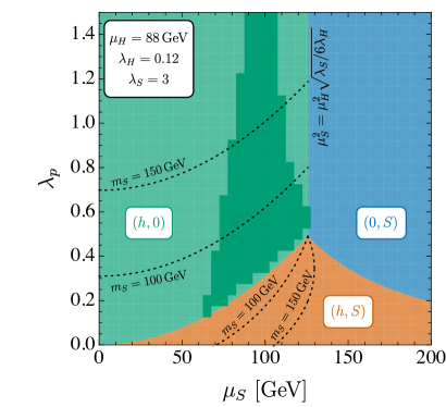
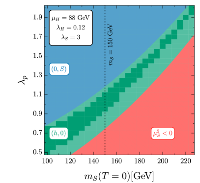
Figure 4: Left: the phase diagram showing which fields obtain a vev in the global minimum of the tree-level effective potential at $T=0$, as a function of $\mu_{S}$ and $\lambda_{p}$. Also shown is $m_{S}(T=0)$ for the physical $(h,0)$ and $(h,S)$ minima. In $(0,S)$ electroweak symmetry is not broken, so it is not physical. Right: the region where a two-step phase transition occurs (green) along with regions where $S$ never obtains a vev (red) and where electroweak symmetry is not broken at $T=0$ (blue) as a function of $m_{S}(T=0)$ and $\lambda_{p}$. Superimposed on both in dark green is the region where cosmoTransitions gives a two-step phase transition for the one-loop effective potential.

Now that we have outlined the two main scenarios of interest, we briefly discuss the parameter space of the effective potential. In fig. 4 (left) we show the phase diagram of the tree-level potential for $\lambda_{S}=3$. The parameter space is divided into regions where at zero temperature the global minimum is one with (green) $(\left\langle h\right\rangle\neq 0,\left\langle S\right\rangle=0)$, (orange) $(\left\langle h\right\rangle\neq 0,\left\langle S\right\rangle\neq 0)$ and (blue) $(\left\langle h\right\rangle=0,\left\langle S\right\rangle\neq 0)$. The blue region does not correspond to our universe, since electroweak symmetry is broken, but either the green or orange region may be physical. In these regions we also plot contours of the $S$ mass at $T=0$. The orange region shows where a one-step phase transition occurs, discussed in section III.1. To simplify calculations we later assume $\lambda_{p}\ll 1$, but the mechanisms we discuss would be seen in the whole orange region.

A two-step phase transition, discussed in section III.2, may occur in the green region. The pixellated region shows points where cosmoTransitions finds that $S$ obtains a vev at some temperature, and then at a later lower temperature, as the SM Higgs obtains its vev, the $S$ vev goes back to zero (also called a vev flip-flop) for the one-loop effective potential. Here, the vev of $h$ gives a contribution to the mass of $S$ and the relation between $m_{S}(T=0)$ and $\mu_{S}$ is

$$m_{S}^{2}(T=0)= \,\frac{\lambda_{p}}{2}\,\langle H\rangle^{2}-\mu_{S}^{2}\,.$$ (23)

We see that when, e.g., $m_{S}(T=0)=150\,\text{GeV}$, only certain values of $\lambda_{p}$ are allowed. This is seen to correspond to fig. 4 (right), where we again plot the green region, now on the $m_{S}(T=0)$ – $\lambda_{p}$ plane. In the lower-right red region, which shows where $\mu_{S}^{2}<0$ at tree-level, the $S$ symmetry is never broken and $S$ never obtains a vev. In the blue region the deepest minima occur when $S$ has a vev and $h$ has no vev, so electroweak symmetry is not broken and this region does not correspond to our universe. The pixellated region again shows where cosmoTransitions calculates that the two-step phase transition successfully completes for the one-loop effective potential. As $\lambda_{S}$ increases, the two-step phase transition region becomes larger. For a given $m_{S}(T=0)$, the $S$ vev and the temperature at which $S$ first obtains a vev both increase with $\lambda_{S}$. Although not shown in these diagrams, $S$ obtains a vev at higher $T$ for larger portal couplings.

IV Finite Temperature Corrections and the Thermal Bath

We now turn to a discussion of the thermal bath. In the hot, early Universe, there is enough energy to produce particles with masses $\lesssim T$. If there are efficient processes which create and destroy a particle, it will come into equilibrium with a number density $n\sim T^{3}$. In this work, we will assume that after inflation and above $T\simeq 100\,\text{TeV}$, there were efficient processes which led to $\chi$, $\psi$ and $S$ to come into equilibrium with the thermal bath. For freeze-in scenarios where $\chi$ does not thermalise in the early universe, see [14].

To determine if certain processes are efficient at keeping the new particles in contact with the thermal bath as the temperature cools, we must calculate the rates of these processes and compare them to the rate of Hubble expansion. The masses which enter the Feynman rules are given by the imaginary part of the self energies, which are modified in the presence of thermal corrections [31, 32]. Although both bosons and fermions obtain these thermal corrections, their different statistics lead to different boundary conditions in the compactified dimension at finite temperature. The bosonic contributions contain a Matsubara zero-mode while the fermionic contributions do not, so the fermionic contributions are subleading to the bosonic contributions. We therefore only include the thermal corrections to the boson masses. However, from eq. 1, we can see that when $S$ has a vev, the effective mass parameter for $\psi$ will receive an extra contribution,

$$m_{\psi}(T)= \,\tilde{m}_{\psi}+y_{\psi}\left\langle S\right\rangle(T)\,,$$ (24)

so $m_{\psi}$ will still depend on temperature. Since we imagine $y_{\chi}$ to be small, we will take $m_{\chi}$ to be temperature independent. Since we will mostly be interested in small mass splittings, we introduce the parameter

$$\Delta= \,\frac{m_{\chi}-\tilde{m}_{\psi}}{m_{\chi}}\,.$$ (25)

These temperature dependent masses mean that kinematic thresholds can open or close as the temperature reduces. In this work, we focus on scenarios where decay and inverse decay of $\chi$, which is only allowed when $m_{\chi}>m_{\psi}(T)+m_{S}(T)$, has a dramatic impact on the resulting dark matter relic abundance. In section VI we consider a scenario where $\chi$ remains in equilibrium until the threshold closes, at which point there are suddenly no processes which keep $\chi$ in contact with the thermal bath and it immediately freezes-out. We call this process instantaneous freeze-out. In this case, the relic abundance is set by the temperature at which the threshold closes, and $m_{\chi}\simeq 30\,T_{\text{End}}$ results in the observed relic abundance. In section VII we consider a scenario where the kinematic threshold is closed at high temperatures and so $\chi$ freezes-out when relativistic. Then, as the finite temperature corrections to $m_{S}$ become smaller, the threshold opens and $\chi$ can decay for some time. Finally, the mass of $\psi$ increases due to $S$ obtaining a vev, closing the threshold and stabilising $\chi$, which we call decaying dark matter. The final relic abundance will then be determined by the amount of decay that has occurred when the threshold closes. The abundance of $\chi$ will approach but not reach equilibrium and produce the observed relic abundance. Ensuring that $\psi$ and $S$ remain in equilibrium means that $\chi\to\psi S$ efficiently depletes the abundance of $\chi$, with the energy density being passed to the thermal bath. In section VIII we consider a similar scenario, but where $S$ is strongly coupled the SM Higgs and a two-step phase transition can occur. In this case, the mass of $\psi$ reduces when $S$ obtains a vev and the kinematic threshold opens, allowing $\chi$ to decay, and closes when the $S$ vev disappears. Again the abundance of $\chi$ will approach but not reach equilibrium and can produce the observed relic abundance. We call this the vev flip-flop.

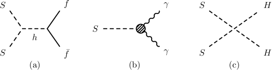
Figure 5: Processes which connect $S$ to the thermal bath.

We now consider the constituents of the thermal bath. The new particles we introduce do not change the evolution of the SM particles, which follow the standard cosmology. For the new particles, we will ensure that $S$ and $\psi$ remain in equilibrium when number changing processes of $\chi$ are active. Although this is not always necessary it will simplify our calculations. We will discuss the precise processes which keep $S$ and $\psi$ in equilibrium in each section, and here give an overview.

In fig. 5 we show three possible ways that $S$ interacts with the SM bath. The processes in fig. 5 (a) and (b) can only keep $S$ in thermal equilibrium when electroweak symmetry (EWS) is broken, while process (c) is always active. Process (a) and (b) will mostly be relevant in sections VI and VII. Process (c) will keep $S$ in thermal equilibrium in section VIII, where EWS is not broken during $\chi$ decay. The annihilation cross sections and decay rates for the processes in fig. 5 are

$$\sigma(SS\to f\bar{f}) =\frac{C_{f}\,\lambda_{p}^{2}\,y_{f}^{2}\,v^{2}}{64\pi s\sqrt{s-4m_{S}^{2}}}\frac{(s-4m_{f}^{2})^{3/2}}{(s-m_{h}^{2})^{2}}\,,$$ (26)

$$\Gamma(S\to\gamma\gamma) =\frac{v^{2}}{16\pi m_{S}}\left(\frac{\lambda_{p}\,v\left\langle S\right\rangle}{m_{h}^{2}-m_{S}^{2}}\right)^{2}|F_{W}^{\gamma\gamma}+F_{f}^{\gamma\gamma}|^{2}\,,$$ (27)

$$\sigma(SS\to HH) =\frac{\lambda_{p}^{2}}{256\pi s}\sqrt{\frac{s-4m_{H}^{2}}{s-4m_{S}^{2}}}\,,$$ (28)

where $C_{f}$ is a colour factor, $y_{f}=m_{f}\,\sqrt{2}/v$ is the Yukawa coupling of the SM fermions to the Higgs, $v$ is the SM Higgs vev, and the factors $F_{W}^{\gamma\gamma}$ and $F_{f}^{\gamma\gamma}$ are given in [33, 34].

Figure 6: Processes which connect $\psi$ to the thermal bath.

In fig. 6 we show processes that may keep $\psi$ in contact with the thermal bath. Since we will be interested in situations where $\chi$ is out of equilibrium, we will choose values of $y_{\psi}$ so that $\psi$ can remain in equilibrium through fig. 6 (b) until the abundance of $\chi$ is fixed. We also want $\chi$ to be the dominant dark matter relic, so we will choose $y_{\psi}$ large enough that $\psi$ freezes-out with less than 10% to the relic abundance. To ensure this, we will need $y_{\psi}\gtrsim 1$ in sections VI and VII and $|y_{\psi}|\gtrsim 4$ in section VIII. This large $y_{\psi}$ also has the benefit of providing a large mass contribution to $\psi$, when $S$ obtains a vev. Process (c) goes as $y_{\chi\psi}^{4}$ and will be too small to keep $\psi$ in equilibrium. In what follows, we will see that $m_{\psi}(T)$ is always smaller than $m_{\chi}+m_{S}(T)$, so the decay process in (a) will always be kinematically forbidden and $\psi$ will only decay via an off-shell $S$. The annihilation cross section for the processes in fig. 6 (b) is

$$\sigma(\psi\bar{\psi}\to SS) \simeq\frac{y_{\psi}^{4}}{64\pi s^{2}(s-4m_{\psi}^{2})}\bigg{[}2(s^{2}+16m_{\psi}^{2}s-32m_{\psi}^{4})\log\bigg{(}\frac{s+\sqrt{s(s-4m_{\psi}^{2})}}{s-\sqrt{s(s-4m_{\psi}^{2})}}\bigg{)}$$

$$\hskip 142.26378pt-4(s+8m_{\psi}^{2})\sqrt{s(s-4m_{\psi}^{2})}\bigg{]}\,,$$ (29)

where we have taken the limit $m_{S}\to 0$. We keep the full $m_{S}$ dependence in our numerical work.

Figure 7: Processes which may connect $\chi$ to the thermal bath. We do not show diagrams involving $\lambda_{p}$, please see text.

Finally, $\chi$ may be in equilibrium through the processes shown in fig. 7. The decay and inverse decay diagram, fig. 7 (a), is proportional to $y_{\chi\psi}^{2}$, while the processes fig. 7 (b) and (c) are at least proportional to $y_{\chi\psi}^{4}$. We will choose $y_{\chi\psi}$ small enough that the processes proportional to $y_{\chi\psi}^{4}$ do not come into equilibrium at the temperatures of interest. The decay rate of the process in fig. 7 (a) is

$$\Gamma(\chi\to\psi S) =\frac{y_{\chi\psi}^{2}}{16\pi}\frac{(m_{\chi}+m_{\psi})^{2}-m_{S}^{2}}{m_{\chi}^{3}}\sqrt{\big{[}m_{\chi}^{2}-(m_{\psi}+m_{S})^{2}\big{]}\big{[}m_{\chi}^{2}-(m_{\psi}-m_{S})^{2}\big{]}}\,.$$ (30)

Note that we do not show $\chi\psi\leftrightarrow S$. Although this channel is kinematically open in the very early universe, when $m_{S}(T)>m_{\chi}+m_{\psi}(T)$, we always take $m_{\chi},\tilde{m}_{\psi}\approx(30-100)\,m_{S}(T=0)$, so this channel will be closed at the temperatures where the abundance of $\chi$ is being set. We also do not show $\psi\leftrightarrow\chi S$ since for the parameter points we consider this decay is always kinematically forbidden.

In (d) - (f) we show channels contributing to $\chi S\leftrightarrow\psi S$. The cross section for the process is

$$\sigma(S\chi\to S\psi) \simeq\frac{y_{\psi}^{2}y_{\chi\psi}^{2}}{32\pi s^{2}(s-m_{\chi}^{2})^{3}}\Big{[}(s-m_{\chi}^{2})(5s^{3}+55m_{\chi}^{2}s^{2}+3m_{\chi}^{4}s+m_{\chi}^{6})$$

$$\hskip 142.26378pt-2s^{2}(s^{2}-18m_{\chi}^{2}s-15m_{\chi}^{4})\log\Big{(}\frac{m_{\chi}^{2}}{s}\Big{)}\Big{]}\,,$$ (31)

where we have taken the limit $m_{\psi}\simeq m_{\chi}$ and $m_{S}\simeq 0$. We have also set $v_{S}=0$ since (f) is subdominant to (d) and (e) for the parameters we consider. In our numerical analysis we use the full expressions. We do however always take $\Gamma_{\psi}=\Gamma_{S}=0$ since the widths of $\psi$ and $S$ are very small. At temperatures near $m_{S}$ but lower than $m_{\chi}$, $n_{S}\langle\sigma(S\chi\to S\psi)v\rangle\sim T^{3}/m_{\chi}^{2}\sim m_{\chi}/x^{3}$ where $x=m_{\chi}/T$, hence the rate of this process will generally be suppressed by a factor $x^{3}$ compared to $\Gamma(\chi\to\psi S)\sim m_{\chi}$. However, the rate can be resonantly enhanced when $m_{S}(T)\approx 0$.

Processes such as $\chi\psi\to S\to SSS$ and $\chi\psi\to S\to SS$ (when $S$ has a vev) are also possible, although the rates will be small as the abundance of $\psi$ will be Boltzmann suppressed at the temperatures of interest, and the intermediate $S$ will be a long way off-shell. We note that although there is in principle mixing between $\chi$ and $\psi$ when $\left\langle S\right\rangle\neq 0$, this mixing will be small and we will ignore its negligible effects. We also neglect diagrams involving $\lambda_{p}$. This coupling is taken to be small in section VI and section VII, while in section VIII these processes lead to a rate significantly smaller than the Hubble rate, due to the $x^{3}$ suppression mentioned above.

V Dark Matter Abundance and the Boltzmann Equations

We will be interested in the abundance of $\chi$ whether or not it is in equilibrium so we will keep track of its abundance using Boltzmann equations. In general the Boltzmann equation for $\chi$ is

$$\dot{n}_{\chi}+3Hn_{\chi} =C[n_{\chi}]\,.$$ (32)

In the parameter space we consider the collision term will have non-negligible contributions from the decay process $\chi\leftrightarrow\psi S$ and the scattering process $\chi S\leftrightarrow\psi S$,

$$C[n_{\chi}] =C_{\chi\leftrightarrow\psi S}[n_{\chi}]+C_{\chi S\leftrightarrow\psi S}[n_{\chi}]\,.$$ (33)

The collision term for the decay process $\chi\leftrightarrow\psi S$ is given by

$$C_{\chi\leftrightarrow\psi S}[n_{\chi}]= \,-\int d\Pi_{\chi}d\Pi_{\psi}d\Pi_{S}(2\pi)^{4}\delta^{4}(p_{\chi}-p_{\psi}-p_{S})\times$$

$$\hskip 56.9055pt\left(\lvert\mathcal{M}_{\chi\to\psi S}\rvert^{2}f_{\chi}(1\pm f_{\psi})(1\pm f_{S})-\lvert\mathcal{M}_{\psi S\to\chi}\rvert^{2}f_{\psi}f_{S}(1\pm f_{\chi})\right)\,,$$ (34)

where $d\Pi_{i}$ is the Lorentz invariant phase space of particle $i$ and $f_{i}$ are their phase space densities. We neglect Pauli-Blocking and Bose-Enhancement, i.e., $(1\pm f_{i})\approx 1$, and assume Maxwell-Boltzmann distributions for $\psi$ and $S$. This is a good approximation for $\psi$, as we will be interested in temperatures much less than the mass of $\psi$, but since these temperatures are similar to the mass of $S$, the full $S$ distribution should be used for more detailed calculations. As we argued above, $\psi$ and $S$ will remain in thermal equilibrium, and we assume with zero chemical potential, during the periods of interest. These assumptions are useful as, when combined with the energy-conservation part of the delta-function, it follows that

$$f_{\psi}f_{S}=e^{-\frac{E_{\psi}}{T}}e^{-\frac{E_{S}}{T}}=e^{-\frac{E_{\chi}}{T}}=f^{eq}_{\chi}\,.$$ (35)

Assuming that the decay process is $CP$ invariant, the collision term then becomes

$$C_{\chi\leftrightarrow\psi S}[n_{\chi}]= \,-\int d\Pi_{\chi}d\Pi_{\psi}d\Pi_{S}(2\pi)^{4}\delta^{4}(p_{\chi}-p_{\psi}-p_{S})\lvert\mathcal{M}_{\chi\to\psi S}\rvert^{2}(f_{\chi}-f^{eq}_{\chi})$$

$$= \,-2\,m_{\chi}\int d\Pi_{\chi}\Gamma_{\chi\rightarrow\psi S}(f_{\chi}-f^{eq}_{\chi})$$

$$= \,-g_{\chi}\int\frac{d^{3}p_{\chi}}{(2\pi)^{3}}\frac{m_{\chi}}{E_{\chi}}\Gamma_{\chi\rightarrow\psi S}(f_{\chi}-f^{eq}_{\chi})\,,$$ (36)

where $g_{\chi}=2$ is the number of degrees of freedom of $\chi$ ($\bar{\chi}$ will satisfy an analogous Boltzmann equation, and will also contribute towards $\Omega_{\chi}$). Note that there is a factor $m_{\chi}/E=1/\gamma$. It appears since particles with higher momenta experience increased time-dilation in the rest frame of the plasma, and so their lifetime is increased. Since we will be interested in situations where almost all $\chi$ decay, this time-dilation in the tail gives an important contribution. To solve this equation in practice, we discretise the integral into bins in momentum space and track the number density in each bin using

$$n_{\chi}^{i}= \,g_{\chi}\int_{p}^{p+\delta p}\frac{d^{3}p^{\prime}}{(2\pi)^{3}}f_{\chi}\,,$$ (37)

which gives

$$C^{i}_{\chi\leftrightarrow\psi S}[n^{i}_{\chi}]= -\frac{\Gamma_{\chi\rightarrow\psi S}}{\gamma^{i}}(n^{i}_{\chi}-n^{eq,i}_{\chi})\,,$$ (38)

where

$$C_{\chi\leftrightarrow\psi S}[n^{i}_{\chi}]= \sum_{i}C^{i}_{\chi\leftrightarrow\psi S}[n^{i}_{\chi}]$$ (39)

For the key results we have checked that changing the number of bins and the highest momentum considered does not significantly change the resulting abundance.

We follow an analogous derivation for the collision term of the scattering process $\chi S\leftrightarrow\psi S$, yielding

$$C^{i}_{\chi S\leftrightarrow\psi S}[n^{i}_{\chi}]= -n_{S}^{eq}\langle\sigma v\rangle(n^{i}_{\chi}-n^{eq,i}_{\chi})\,.$$ (40)

where the thermally averaged cross section for non-identical initial state particles is given by

$$\langle\sigma v\rangle= \,\frac{1}{8Tm_{\chi}^{2}m_{S}^{2}K_{2}(\frac{m_{\chi}}{T})K_{2}(\frac{m_{S}}{T})}\cdot$$

$$\int_{(m_{\chi}+m_{S})^{2}}^{\infty}\sigma\frac{[s-(m_{\chi}-m_{S})^{2}]}{\sqrt{s}}(s-(m_{\chi}+m_{S})^{2})K_{1}\left(\frac{\sqrt{s}}{T}\right)ds\,,$$ (41)

where $K_{1,2}$ are modified Bessel functions of the first and second kind, see, for example, [35]. Although we do not need to discretise this collision term in momentum space, we write it in this way to combine it with the collision term for decay. Writing

$$\Gamma_{\chi S\rightarrow\psi S}= \,n_{S}^{eq}\langle\sigma v\rangle$$ (42)

and introducing the yield, $Y_{\chi}=n_{\chi}/s$, we can write

$$\frac{dY_{\chi}^{i}}{dx}=-\left(\frac{\Gamma_{\chi\rightarrow\psi S}}{\gamma^{i}}+\Gamma_{\chi S\rightarrow\psi S}\right)(Y^{i}_{\chi}-Y^{eq,i}_{\chi})\frac{dt}{dx}\,,$$ (43)

where $x=m_{\chi}/T$.

We will be interested in tracking the relic abundance through changes in the effective number of relativistic degrees of freedom, $g_{\ast}(T)$, so we use the conservation of entropy to write

$$\frac{dT}{dt}= \,\frac{-HT}{1+\frac{T}{3g_{\ast}(T)}\frac{dg_{\ast}(T)}{dT}}\,.$$ (44)

We then obtain a differential equation for each momentum bin,

$$\frac{dY_{\chi}^{i}}{dx}=-\frac{1+{\frac{m_{\chi}}{3xg_{\ast}(T)}\frac{dg\ast(T)}{dT}}}{Hx}\left(\frac{\Gamma_{\chi\rightarrow\psi S}}{\gamma^{i}}+\Gamma_{\chi S\rightarrow\psi S}\right)(Y^{i}_{\chi}-Y^{eq,i}_{\chi})\,.$$ (45)

Although $\chi$ is at times out of equilibrium we check that it never dominates the energy density of the universe, so we can use the usual radiation dominated Hubble expansion of the universe.

VI Instantaneous Freeze-out

With this machinery, we can now turn to exploring various mechanisms of dark matter production. In this section, we will focus on the region of parameter space where the new scalar field exhibits a one-step phase transition, section III.1, and the Yukawa coupling $y_{\chi\psi}$ $\sim 10^{-7}$ is large enough to put $\chi$ into equilibrium. We will assume $m_{\chi}\approx m_{\psi}\approx(30-100)\times m_{S}(T=0)$. This both produces the observed relic abundance of $\chi$ and means that at $T\approx\mu_{S}$ both initial state particles in the 2–to–2 processes $\chi\chi\to\psi\psi$, $\chi\chi\to SS$ and $\chi\psi\to SS$ are significantly Boltzmann suppressed, dramatically reducing the rate $n\left\langle\sigma v\right\rangle$, so these processes can not keep $\chi$ in equilibrium. We will further assume that $\lambda_{p}=10^{-5}-10^{-3}$ and $y_{\psi}=2$. These couplings ensure that $S$ and $\psi$ remain in equilibrium until the abundance of $\chi$ is set. $S$ stays in equilibrium through $SS\leftrightarrow HH$ when it is much heavier than the Higgs, and through $SS\leftrightarrow\bar{f}f$, where $f$ is a SM fermion, when it is much lighter than the Higgs and electroweak symmetry is broken at the temperatures of interest. For $S$ lighter than the muon, the Yukawa coupling becomes too small to keep $S$ in equilibrium, putting a lower limit on the $S$ masses we consider. The process $S\leftrightarrow\gamma\gamma$ can also keep $S$ in equilibrium when $S$ has a vev, near $T_{E}$. The dark sector fermion $\psi$ remains in equilibrium through $\psi\psi\leftrightarrow SS$.

This mechanism, and the others we present in this paper, depend heavily on the opening and closing of a kinematic threshold, which occurs due to the temperature dependence of the masses of $S$ and $\psi$. As such, we will be interested in the region of parameter space where $\chi$ and $\psi$ have a similar mass, as is natural if they obtain their masses from the same mechanism. In this example we will choose $m_{\chi}=77\,\text{GeV}$, $\tilde{m}_{\psi}=74\,\text{GeV}$. We take $y_{\chi\psi}=5\times 10^{-8}$ for the new Yukawa coupling while here and elsewhere we will take $y_{\chi}\approx 0$. For the new scalar we will first choose $m_{S}(T=0)=1\,\text{GeV}$ and $\lambda_{S}=1$. We can see in fig. 1 (right) that with these parameters, $\left\langle S\right\rangle(T=0)\approx 1.7\,\text{GeV}$, so $m_{\psi}$ will increase from $74\,\text{GeV}$ at high temperatures to $74\,\text{GeV}+y_{\psi}\left\langle S\right\rangle(T=0)\approx 77.4\,\text{GeV}$ at $T\approx 0$. At high temperatures, $\psi$ is the lightest dark sector particle, while at $T\approx 0$, $\chi$ takes this role.

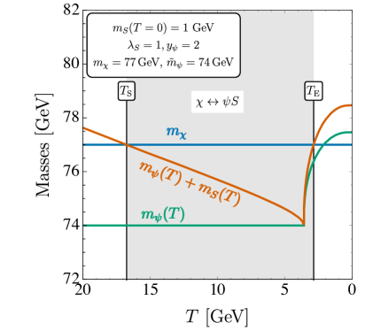
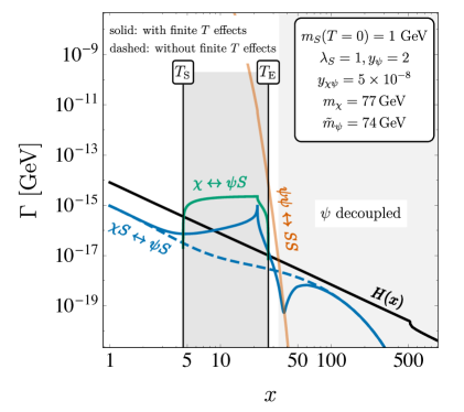
Figure 8: Left: the masses of $\chi$ and $\psi$ as a function of temperature, along with the period where the channel $\chi\leftrightarrow\psi S$ is kinematically allowed. Right: The rates of processes which at some $x$ are larger than the Hubble expansion rate, $H$. In dashed blue we show the rate of $\chi S\leftrightarrow\psi S$ if finite temperature effects are ignored. In light grey we show the period where $\psi$ is decoupled from the thermal bath.

The temperature dependent masses for this set of parameters are shown in fig. 8 (left). We see that at high temperatures, $m_{S}$ receives a large correction and the channel $\chi\leftrightarrow\psi S$ is closed. As the temperature reduces, the $T$ dependent corrections become smaller and the mass of $S$ reduces. The channel $\chi\leftrightarrow\psi S$ becomes active at $T\approx 17\,\text{GeV}$. This continues while $S$ goes through its phase transition, where $S$ obtains a vev and its mass starts to increase. The vev contributes to $m_{\psi}$, so both of these effects act to close the channel. At $T_{\text{E}}\approx 3\,\text{GeV}$, $m_{\chi}$ becomes smaller than $m_{\psi}(T)+m_{S}(T)$, so the process $\chi\leftrightarrow\psi S$ becomes kinematically forbidden. At $T=0$, $m_{\chi}<m_{\psi}$, so $\chi$ is the lightest dark sector particle and cannot decay, even via off-shell processes.

In fig. 8 (right) we show the rates of key processes along with the expansion rate of the universe, $H$, as a function of $x=m_{\chi}/T$. When the rate of a process is much larger than $H$ then it will effectively keep $\chi$ or $\psi$ in equilibrium, but when it is much smaller then it will not. We see that between $T_{\text{S}}$ to $T_{\text{E}}$, $\chi\leftrightarrow\psi S$ is the dominant process and will act to put $\chi$ into equilibrium. The process $\chi S\leftrightarrow\psi S$ may also have a rate larger than the expansion rate of the universe, and will contribute. The rate of $\chi S\leftrightarrow\psi S$ shows two resonant features, one at $x\sim 20$, when $m_{S}\sim 0$ and the propagator $\psi$ can be nearly on-shell, and another at $x\sim 40$, when $m_{\psi}\sim m_{\chi}$ and diagrams (d) and (e) in fig. 7 destructively interfere. Although $\psi$ is kept in chemical equilibrium via $\psi\psi\leftrightarrow SS$ until $T_{E}$, it decouples soon after at $x\sim 30$. Once $\psi$ has departed from chemical equilibrium, the relic abundance of $\chi$ cannot be reduced, since any $\psi$ produced will simply decay back to $\chi$. We also show the rate of $\chi S\leftrightarrow\psi S$ if finite temperature effects are ignored. We see that in this case the $\chi S\leftrightarrow\psi S$ rate is always smaller than the Hubble rate, so $\chi$ will freeze-out while relativistic. All other processes involving $\chi$ have rates orders of magnitude smaller than the Hubble rate.

In fig. 9 (left) we show the evolution of the yield of $\chi$. At small $x$ there are no processes connecting $\chi$ to the thermal bath with a rate larger than the Hubble rate, so $\chi$ freezes-out. Then, at $T_{S}$ the rate of $\chi\leftrightarrow\psi S$ (and later $\chi S\leftrightarrow\psi S$) becomes larger than the Hubble rate and the $\chi$ yield comes back into equilibrium. At $T_{\text{E}}$, however, these channel suddenly becomes inefficient and, since there are no longer any processes keeping $\chi$ in equilibrium, it instantaneously freezes-out. We see that in this scenario, the relic abundance of $\chi$ is set not by usual, smooth freeze-out, resulting from an interplay between a slowly varying annihilation or decay rate and the Hubble rate, but by a sudden and dramatic change in rates. If these finite temperature effects are ignored, the final abundance is overestimated by $\approx 10$ orders of magnitude, since the rate of the most relevant process $\chi S\leftrightarrow\psi S$ remains below the Hubble rate throughout.

This means that the resulting yield is not a function of the coupling constant (provided the assumptions above are satisfied), but only of the mass of the dark matter candidate and $T_{\text{E}}$. The final yield is simply given by

$$Y_{\chi}^{\infty}= \,Y_{\chi}^{\text{Eq.}}(T=T_{\text{E}})\,,$$ (46)

which is only a function of $m_{\chi}$ and $T_{\text{E}}$ (which in turn is a function of $\tilde{m}_{\psi}$, $y_{\psi}$ and the effective potential).

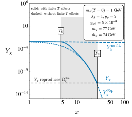
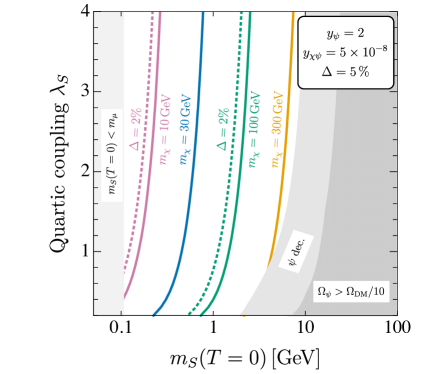
Figure 9: Left: the evolution of the yield of $\chi$ as a function of temperature (solid) with the equilibrium yield of $\chi$ (dotted) and the yield calculated without accounting for the finite temperature effects (dashed). Also shown is the yield which is required to obtain the observed relic abundance of $\chi$ (black, dashed). Right: the required values of $m_{S}(T=0)$ and $\lambda_{S}$ for various $\chi$ masses, for $\Delta=5\%$ and $2\%$. In the left light-grey region $S$ is not in equilibrium throughout the decay of $\chi$, in the central grey region $\psi$ decouples before $T_{\text{E}}$, while in the right dark-grey region $\psi$ is not a subdominant relic.

We now consider the parameter space of this mechanism. Rather than considering the full 7-dimensional parameter space, we explore the impact of varying one or two parameters at a time. The final relic abundance is insensitive to $y_{\chi\psi}$ as long as $\chi\leftrightarrow\psi S$ is fast enough to keep $\chi$ in equilibrium (providing a lower bound on $y_{\chi\psi}$) and as long as $\chi S\leftrightarrow\psi S$ does not significantly deplete $\chi$ after $T_{\text{E}}$ (providing an upper bound on $y_{\chi\psi}$). For the benchmark values of the other parameters, this is satisfied for $3\times 10^{-8}<y_{\chi\psi}<1\times 10^{-7}$. As discussed above, the mechanism occurs while $y_{\psi}$ is large enough to keep $\psi$ in equilibrium while the processes $\chi\leftrightarrow\psi S$ and $\chi S\leftrightarrow\psi S$ occur. If $\psi$ goes out of equilibrium before $T_{\text{E}}$, the processes will not reduce the energy density in the dark sector and, once $m_{\chi}<m_{\psi}$, $\psi$ will decay to $\chi$. In this variation of the mechanism, the relic abundance is set by the freeze-out of $\psi$, not via the dramatic change in the rates of $\chi\leftrightarrow\psi S$ and $\chi S\leftrightarrow\psi S$ at $T_{\text{E}}$. However, in both scenarios, the Yukawa coupling $y_{\chi}$ should be small enough that the 2–to–2 process $\chi\chi\leftrightarrow SS$ is inefficient by $T_{\text{E}}$ or when $\psi$ freezes-out.

In fig. 9 (right) we show the mass of $\chi$ required to produce the observed relic abundance, for $\Delta=5\%$ and $2\%$. We see that $m_{\chi}$ is $30-100$ times larger than $m_{S}(T=0)$, depending on $\lambda_{S}$. Although $m_{S}(T=0)$ depends on $\mu_{S}$, the $S$ vev also depends inversely on the square root of $\lambda_{S}$. This means that as $\lambda_{S}$ becomes smaller, the $S$ vev gets larger. The temperature of the phase transition, which is close to $T_{\text{E}}$, also increases. These two effects mean that $m_{\chi}$ has to increase to compensate. Reducing the mass splitting $\Delta$ has the effect of requiring a larger $m_{\chi}$. This is because a smaller $\Delta$ means that the important 1-to-2 process closes at a higher $T$, so $Y_{\chi}^{\text{Eq.}}(T=T_{\text{E}})$ becomes larger. To yield the observed relic abundance, $m_{\chi}$ then has to increase. If the mass splitting is much larger than $5\%$ then the $\left\langle S\right\rangle$ contribution to $m_{\psi}$ at $T=0$ is not large enough to close the mass gap, so $m_{\chi}>m_{\psi}(T=0)$. As mentioned above, if $S$ is lighter than the muon then it is not in equilibrium throughout the process, so the decay does not reduce the energy density of the dark sector. For $m_{\mu}<m_{S}(T=0)\lesssim 1\,\text{GeV}$, either $\lambda_{p}$ must be reduced below $\lambda_{p}=10^{-3}$ or there is some tuning between the $\mu_{S}^{2}$ term and $\lambda_{p}\left\langle h\right\rangle S^{2}/4$ to achieve this low mass. If $\lambda_{p}$ is reduced, care must be taken that $S$ remains in equilibrium throughout. We find that we require $\lambda_{p}\gtrsim 10^{-5}$ in this low $m_{S}$ region of parameter space. On the other hand, as $m_{S}(T=0)$ increases, $m_{\psi}$ also increases (along with $m_{\chi}$). For the parameters chosen, when $\psi$ is heavy it can freeze-out (at $T=T_{\psi}^{\text{f.o.}}$) at temperatures higher than $T_{\text{E}}$. In this case, dark sector fermion number conservation implies that the $\chi$ abundance is given by

$$Y_{\chi}^{\infty}= \,Y_{\chi}^{\text{Eq.}}(T=T_{\psi}^{\text{f.o.}})\,.$$ (47)

With $y_{\psi}=2$, if $m_{\psi}\gtrsim 1\,\text{TeV}$ then $\psi$ will freeze-out with a relic abundance greater than 10% of the observed relic abundance, so the mechanism we are discussing will not be the dominant mechanism in setting the relic abundance. The quartic coupling $\lambda_{S}$ can become larger than 4 but at some point it becomes non-perturbative and the one-loop analysis breaks down.

VII Decaying Dark Matter with a One-Step Phase Transition

Now we continue to consider the region of parameter space where the new scalar field exhibits a one-step phase transition, discussed in section III.1, but assume a smaller Yukawa coupling, $y_{\chi\psi}\lesssim 10^{-7}$. With a coupling this small, $\chi$ either freezes-out while relativistic or never comes into equilibrium with the thermal bath (as in the freeze-in scenario [14]). Here we will assume that there is some UV physics which connected $\chi$ to the thermal bath after reheating, so that $\chi$ was in equilibrium at high temperatures. In this scenario $\chi$ will have frozen out when relativistic, then $\chi\leftrightarrow\psi S$, and to a lesser extent $\chi S\leftrightarrow\psi S$, bring $\chi$ towards equilibrium after $T_{S}$. This means that $\chi$ will deplete and its abundance will approach the equilibrium abundance. At $T_{\text{E}}$ these process become inefficient and the yield of $\chi$ stabilises. We will require $m_{\chi}\approx m_{\psi}\approx 30\,m_{S}$ to obtain the observed relic abundance. With these masses and couplings the rates of $\chi\leftrightarrow\psi S$ and $\chi S\leftrightarrow\psi S$ are the only processes to ever have a rate greater than the Hubble rate. As discussed in section VI, $\psi$ and $S$ remain in equilibrium throughout the decay process.

To describe the mechanism in this case, we will keep the same scalar parameters chosen above but slightly increase the dark sector fermion masses (we take in this example $m_{\chi}=90\,\text{GeV}$ and $\tilde{m}_{\psi}=87\,\text{GeV}$) and reduce the Yukawa coupling to $y_{\chi\psi}\lesssim 10^{-7}$ (here we take $y_{\chi\psi}=2.57\times 10^{-8}$). The temperature dependence of the masses is shown in fig. 10 (left). We see that with these parameter choices, fig. 8 (left) is simply shifted to slightly higher masses and the channel $\chi\leftrightarrow\psi S$ is open in the same temperature range, $17\,\text{GeV}\gtrsim T\gtrsim 3\,\text{GeV}$.

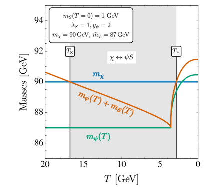
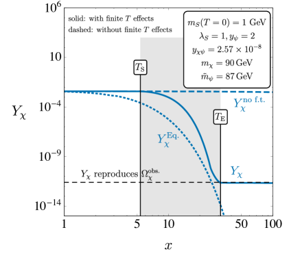
Figure 10: Left: the masses of $\chi$ and $\psi$ as a function of temperature, along with the period where the channel $\chi\leftrightarrow\psi S$ is kinematically allowed. Right: the evolution of the yield of $\chi$ as a function of temperature (solid) with the equilibrium yield of $\chi$ (dotted) and the yield calculated without accounting for the finite temperature effects (dashed). Also shown is the yield which is required to obtain the observed relic abundance of $\chi$ (black, dashed).

In fig. 10 (right) we show the evolution of the yield of $\chi$ with $x$. As expected for $y_{\chi\psi}\lesssim 10^{-7}$, $\chi$ freezes-out while it is still relativistic. However, at $T_{\text{S}}\approx 17\,\text{GeV}$ the channel $\chi\leftrightarrow\psi S$ becomes kinematically allowed and the $\chi$ abundance reduces, approaching the equilibrium curve. The $\chi S\leftrightarrow\psi S$ channel also contributes to a lesser extent. However, in this case, the rate is not fast enough to reach equilibrium and $Y_{\chi}$ remains larger than $Y_{\chi}^{\text{Eq.}}$ at all times. This continues until the channel closes at $T_{\text{E}}\approx 3\,\text{GeV}$ and the yield of $\chi$ becomes fixed until the present day, reproducing the observed relic abundance.

In this case the final yield is not set by $Y_{\chi}^{\text{Eq.}}$ at $T_{\text{E}}$, but by the amount of $\chi$ that has decayed in the period from $T_{\text{S}}$ to $T_{\text{E}}$. This depends on $y_{\chi\psi}$ and on the temperature dependent masses of the particles. As such there is no simple formula for calculating the resulting abundance; the final abundance must be calculated numerically.

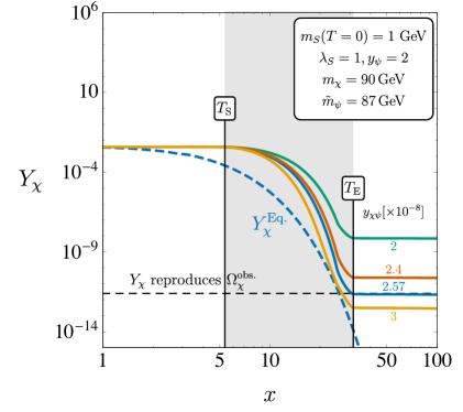
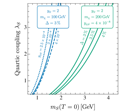
Figure 11: Left: the evolution of the yield for different values of $y_{\chi}$ (solid lines). The equilibrium abundance of $\chi$ is dashed blue while the yield required to reproduce the observed DM relic abundance is black dashed. Right: the $m_{S}(T=0)$ and $\lambda_{S4}$ which reproduce the observed DM relic abundance for different parameter choices. For the dotted line $\psi$ freezes-out before $T_{\text{E}}$, while for the dashed line $\chi$ returns to equilibrium.

We now vary the parameters of the model to see their dependence. We first point out that the relic abundance obtained is exponentially sensitive to the coupling $y_{\chi\psi}$. In fig. 11 (left) we show the evolution of the yield for different values of $y_{\chi\psi}$. As seen above, for a coupling of $y_{\chi\psi}=2.57\times 10^{-8}$ we obtain $\Omega_{\chi}h^{2}=0.12$. With a smaller coupling of $y_{\chi\psi}=2\times 10^{-8}$ we obtain $\Omega_{\chi}h^{2}\sim 340$, $y_{\chi\psi}=2.4\times 10^{-8}$ gives $\Omega_{\chi}h^{2}=1.2$, while $y_{\chi\psi}=3\times 10^{-8}$ gives $\Omega_{\chi}h^{2}=0.015$. We see that a $\approx 10\%$ change in the coupling changes the final abundance by an order of magnitude. As such, this mechanism provides no answer to the coincidence problem (that $\Omega_{\chi}\approx 5\,\Omega_{\text{SM}}$).

In fig. 11 (right) we vary the effective potential, $m_{\chi}$, $y_{\chi\psi}$ and $\Delta$, and plot the curve where the observed relic abundance is reproduced. We see that the observed abundance is reproduced for $m_{\chi}\approx(50-200)\times m_{S}(T=0)$. As in section VI, a smaller quartic coupling $\lambda_{S}$ results in a larger $S$ vev and phase transition temperature, resulting in a heavier $\chi$. Increasing the mass of $S$ similarly provides a larger vev and a larger phase transition temperature, requiring a heavier $\chi$. A larger $y_{\chi\psi}$ means that $\chi$ depletes faster so $T_{\text{E}}$ needs to occur at a higher temperature, which is achieved with a heavier $S$ or a smaller $\lambda_{S}$. Similarly, a larger $\Delta$ means that $T_{\text{E}}$ is naturally lower, so this needs to be compensated with a larger $S$ mass or a smaller $\lambda_{S}$. When $S$ is lighter than the muon, $S$ must couple via a first generation SM Yukawa coupling, which is so small that $S$ does not stay in equilibrium throughout the process. The upper bound on $m_{S}$ is again determined by requiring that $\psi$ freezes-out as a subdominant relic, around $m_{\psi}\approx 1\,\text{TeV}$, but we show just a small region of the possible parameter space to demonstrate the impact of varying $y_{\chi\psi}$ and $\Delta$. It may also happen, as in section VI, that $\psi$ freezes-out before $T_{\text{E}}$. This occurs for the dotted line ($y_{\chi\psi}=2.5\times 10^{-8}$), since the lower $m_{S}(T=0)$ reduces $T_{\text{E}}$ below the $\psi$ decoupling temperature. For the dashed line ($y_{\chi\psi}=4\times 10^{-8}$) the coupling is large enough that $\chi$ returns to equilibrium, so the situation is as discussed in section VI. The quartic coupling $\lambda_{S}$ can also in principle be increased to the perturbativity limit.

VIII Decaying Dark Matter with a Two-Step Phase Transition

Finally we consider the region of parameter space where $\lambda_{p}$ is not negligible, but $\mathcal{O}(1)$. As discussed in section III.2, this can lead to a two-step phase transition where first the new scalar $S$ obtains a vev and later, at the onset of electroweak symmetry breaking (EWSB), the SM Higgs obtains a vev and $\left\langle S\right\rangle$ goes to zero. This two-step phase transition only occurs in the region of parameter space where $\mu_{S}\approx\mu_{H}$, which means that $m_{S}(T=0)=\mathcal{O}(100\,\text{GeV})$. To maintain $m_{\chi}\gtrsim 30\,m_{S}(T=0)$, so that the abundance is set by decay, we require $m_{\chi},m_{\psi}\approx 4$ – $5\,\text{TeV}$. Since $\psi$ is now quite heavy, it will naturally freeze-out with a large relic abundance. To counter this and to ensure that $\psi$ is a subdominant relic, we have to take $|y_{\psi}|\gtrsim 4$ which, while large, is still perturbative. However, corrections from higher orders in the perturbative expansion will not be as small as usually assumed. With this two-step phase transition, we will take $y_{\psi}<0$, so that $\psi$ becomes lighter when $S$ obtains a vev. This allows the channel $\chi\leftrightarrow\psi S$ to open when $S$ obtains a vev, and to close when the $S$ vev goes to zero. This situation can lead to the observed relic abundance either by instantaneous freeze-out when $y_{\chi\psi}$ is $\sim 10^{-7}$, as in section VI, or with a period of DM decay with $y_{\chi\psi}\lesssim 10^{-7}$, as in section VII. Here we choose to explore the latter, to make a connection with the mechanism described in [12].

In [12] it was shown that a new $su(2)_{L}$ triplet scalar $S_{3}$ offers decay channels to a singlet DM candidate when there are two extra dark sector $su(2)_{L}$ triplet fermions, $\psi_{3}$ and $\psi_{3}^{\prime}$. In this case, there are the channels $\chi\leftrightarrow\psi_{3}^{+}W^{-}$ and $\chi\leftrightarrow\psi_{3}^{\prime+}W^{-}$ in addition to the process discussed in the present work, $\chi\leftrightarrow\psi_{3}S_{3}$. However, as we demonstrate here, this extra structure is not required and the observed relic abundance can be obtained through the $\chi\leftrightarrow\psi S$ process.

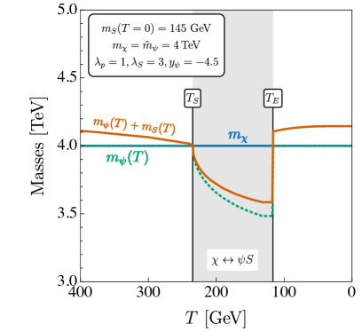
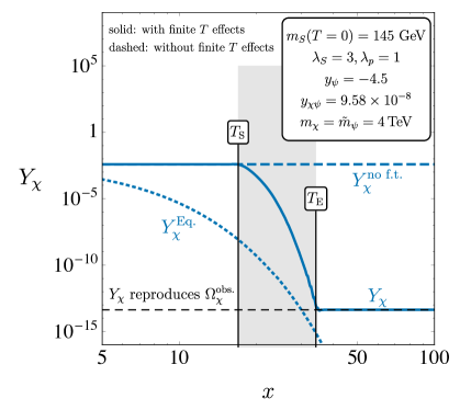
Figure 12: Left: the masses of $\chi$ and $\psi$ as a function of temperature, along with the period where the channel $\chi\leftrightarrow\psi S$ is kinematically allowed. Right: the evolution of the yield of $\chi$ as a function of temperature (solid) with the equilibrium yield of $\chi$ (dashed) and the yield which is required to obtain the observed relic abundance of $\chi$ (black, dashed).

In fig. 12 we again show (left) the masses as a function of $T$. Recall that $m_{\psi}(T)=\tilde{m}_{\psi}+y_{\psi}\left\langle S\right\rangle$. We see that in this case $m_{\chi}=m_{\psi}=4\,\text{TeV}$, as long as $\left\langle S\right\rangle=0$, c.f., fig. 3. However, when $\left\langle S\right\rangle\neq 0$, there is a large negative contribution to $m_{\psi}$, since $y_{\psi}<0$. The mass of $S$ also becomes relatively small between $T_{\text{S}}$ and $T_{\text{E}}$, so the channel $\chi\leftrightarrow\psi S$ opens. At $T_{\text{E}}$ there is a first-order phase transition and, since $\left\langle S\right\rangle$ goes to zero, $m_{\psi}(T)$ returns to $\tilde{m}_{\psi}$ and the channel $\chi\leftrightarrow\psi S$ abruptly closes.

As mentioned above, the large Yukawa coupling $|y_{\psi}|\gtrsim 4$ ensures that $\psi$ remains in equilibrium throughout the depletion of $\chi$. $S$ has a large portal coupling so can easily stay in equilibrium via $SS\leftrightarrow HH$. As discussed in section IV, the rates of all 2–to–2 processes involving $\chi$, except $\chi S\leftrightarrow\psi S$, remain significantly below the Hubble rate at all times. The rate of $\chi S\leftrightarrow\psi S$ is suppressed when $m_{\chi}\approx m_{\psi}(T)$ but enhanced when $m_{S}(T)\approx 0$. This means that the rate of $\chi S\leftrightarrow\psi S$ can be larger than the Hubble rate in the period where $S$ obtains a vev. Although it remains subdominant to $\chi\leftrightarrow\psi S$ in this period, we include it in out numerical calculations. Like $\chi\leftrightarrow\psi S$, the rate of $\chi S\leftrightarrow\psi S$ abruptly reduces below the Hubble rate at $T_{\text{E}}$.

In fig. 12 (right) we see the yield of $\chi$ as a function of $x$. As in section VII, $\chi$ initially freezes-out when relativistic, before beginning to deplete at $T_{\text{S}}$. The depletion continues until it abruptly halts at $T_{\text{E}}$. It stops more abruptly than in section VII due to the first-order phase transition, which quickly changes the mass of $\psi$ at $T_{\text{E}}$. After $T_{\text{E}}$, $\chi$ stabilises and the yield remains constant. We see that there is a choice of $y_{\psi}$ such that the observed relic abundance is obtained. Again, once $\chi$ has departed from equilibrium at high temperatures, it does not return to equilibrium. We see that properly accounting for these finite temperature effects is essential for calculating the correct abundance.

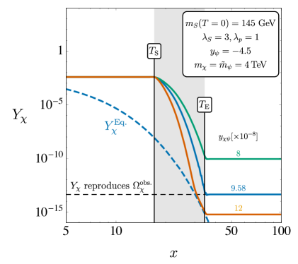
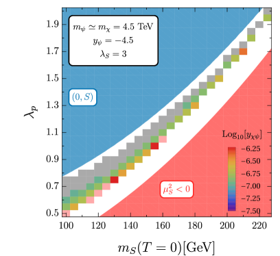
Figure 13: Left: the evolution of the yield for different values of $y_{\chi}$. Right: the $y_{\chi}$ required to produced the observed relic abundance in the $\lambda_{S}$ – $m_{S}(T=0)$ plane. In the red region $S$ does not obtain a vev, while in the blue region electroweak symmetry is not broken at $T=0$. The grey pixels show where $\psi$ freezes-out before $T_{\text{E}}$ while at the pink pixels the equilibrium abundance of $\chi$ at $T_{\text{E}}$ is too large for $Y_{\chi}$ to reduce to the observed value.

We now consider the parameter space of this scenario. In fig. 13 (left) we show the evolution of the yield for different Yukawa couplings $y_{\chi\psi}$. We see that the final yield is again exponentially sensitive to this coupling. A small change in the coupling results in an orders of magnitude change in the final yield. When the Yukawa coupling is $y_{\chi\psi}\gtrsim 1.2\times 10^{-7}$ we see that the rate is fast enough to bring $\chi$ back into equilibrium. We here explicitly see the relationship between instantaneous freeze-out and decaying dark matter. If $\chi$ does go back into equilibrium, the final abundance is simply set by the equilibrium abundance at $T_{\text{E}}$, as in section VI. We note that the abundance of $\chi$ cannot go below the equilibrium abundance with this mechanism.

In fig. 13 (right) we show the value of $y_{\chi\psi}$ required to produce the equilibrium abundance of $\chi$ in the $m_{S}(T=0)$ – $\lambda_{p}$ plane. We have increased the $\chi$ and $\psi$ mass to 4.5 TeV, since otherwise the equilibrium abundance of $\chi$ is above the observed abundance at $T_{\text{E}}$ for many points, meaning that decay cannot set the abundance (this is still the case for some points, shown in pink). In the red region, $\mu_{S}^{2}$ is negative so $S$ never obtains a vev and $\chi$ does not decay. In the blue region, the deepest minima at zero temperature have $\left\langle S\right\rangle\neq 0$ and $\left\langle h\right\rangle=0$, so electroweak symmetry is not broken (i.e., this region is unphysical). In the region between these curves we show a pixellated region where the universe successfully transitions to the EWSB minimum. We see that larger couplings $y_{\chi\psi}$ are required near the red region, where symmetry breaking is weak and $S$ only obtains a vev for a short amount of time. Closer to the blue region the required Yukawa coupling is smaller, as there is a longer amount of time in which $\chi$ can decay. The grey pixels show where $\psi$ freezes-out before $T_{\text{E}}$.

We do not show the variation with $m_{\chi}$ and $m_{\psi}$ since this mechanism only works in a relatively small window. If these masses become much larger, then $\psi$ is no longer a subdominant relic. On the other hand, since $T_{\text{E}}\approx 100\,\text{GeV}$, if the fermions are much lighter, then the equilibrium abundance at $T_{\text{E}}$ is too large and $\chi$ overcloses the universe.

IX Experimental Constraints

We now briefly consider experimental tests of the model in different regions of its parameter space. The usual probes of dark matter, direct and indirect detection of the galactic population and direct dark matter production at colliders, may be effective for the parameter space for instantaneous freeze-out, considered in section VI. However, since in this section the relic abundance is not determined by $y_{\chi\psi}$, there is no expectation of a coupling of a certain size (as there is in typical freeze-out scenarios). In sections VII and VIII, where we consider decaying dark matter, these searches are hindered by the small coupling $y_{\chi\psi}$, as is common for freeze-in models. However, direct detection is beginning to probe even these small couplings [36].

Aside from directly searching for $\chi$, the model may first be probed via its other particle content. In all cases the energy density in $\chi$ must be passed to the SM thermal bath. This means that $S$ and $\psi$ must be in equilibrium while the $\chi\leftrightarrow\psi S$ channel is open, which in turn means that the $S^{2}|H|^{2}$ portal coupling must be $\approx 10^{-3}$ (although for masses less than a GeV it could be as small as $10^{-5}$). If $S$ is lighter than $m_{h}/2$, it may be detected by precision measurements of the Higgs. The current limit excludes $\lambda_{p}\gtrsim 10^{-2}$ [37, 38] while future colliders such as the ILC and CEPC will probe $\lambda_{p}\gtrsim 10^{-3}$ [39, 40, 41]. Pairs of heavy $S$ particles may be produced via an off-shell Higgs at proton colliders. A future $100\,\text{TeV}$ machine with $30\text{ ab}^{-1}$ of integrated luminosity will be able to exclude the two-step phase transition region of section VIII at $2\sigma$ but not discover an $S$ in this region at $5\sigma$ [42, 43, 44]. It will not be able to probe the scalar sector in sections VI and VII.

In sections VI and VII, any remaining $\psi$ and $S$ can decay, so these will not make any of the dark matter relic abundance. However, in section VIII there is a subdominant population of both $\psi$ and $S$ ($S$ has no vev at $T=0$ so the $\mathbb{Z}_{2}$ symmetry may be intact). Assuming that the $\mathbb{Z}_{2}$ symmetry is not softly broken by effects from particles beyond this simple model, the subdominant populations of $S$ and $\psi$ may be detected by direct or indirect detection experiments. However, the rates seen in these experiments depend on their abundances, which are unconnected to the $\chi$ abundance.

In the scenario in section VIII there is a first-order phase transition, as $h$ obtains a vev and $S$ loses its vev. If this phase transition is strong enough there is the interesting possibility of detecting a stochastic gravitational wave background resulting from the first order phase transition in upcoming space based interferometers such as LISA [45].

X Conclusions

In this work we have explored the impact of finite temperature corrections on the relic abundance of a simple model of dark matter, which consists of two dark sector fermions (one being a dark matter candidate, $\chi$, and a further dark sector fermion $\psi$) and a new scalar, $S$. We calculate the leading finite temperature effects, using the effective potential of the new scalar and the SM Higgs, and track the dark matter abundance using Boltzmann equations. We emphasise that in different regions of parameter space the new scalar can either simply obtain a vev (which we focus on in sections VI and VII), or pass through a two-step phase transition during EWSB (section VIII). These finite temperature effects provide corrections to the scalar and fermion masses. We assume that $\chi$ was in equilibrium at high temperatures and focus on regions of parameter space where decays and inverse decays $\chi\leftrightarrow\psi S$ are kinematically allowed for a period of time. We also ensure that $S$ and $\psi$ remain in equilibrium with the SM thermal bath during the time of interest. We have explored the parameter space of the model and identified different regions where finite temperature effects lead to non-standard mechanisms of dark matter production.

In section VI we discussed instantaneous freeze-out and considered the parameter space where $\chi$ can quickly come into equilibrium through the processes $\chi\leftrightarrow\psi S$ and $\chi S\leftrightarrow\psi S$. When these channels abruptly become inefficient, $\chi$ instantaneously freezes-out, resulting in a tight relationship between the temperature of decoupling and the resulting relic abundance. We find viable dark matter candidates in the range $m_{\chi}\approx(3\,\text{GeV}-300\,\text{GeV})$, although $\chi$ and $\psi$ should have similar mass (at the 5% level) to avoid significant fine tuning. However, the final abundance depends exponentially on the temperature at which the $\chi\leftrightarrow\psi S$ and $\chi S\leftrightarrow\psi S$ channels become inefficient.

In section VII we discuss the case where $\chi$ is only weakly coupled to the thermal bath and consider decaying dark matter via a one-step phase transition. In this case, rather than quickly coming into equilibrium, the yield of $\chi$ slowly approaches the equilibrium yield. The final abundance of $\chi$ depends on all of the model parameters in a complicated manner. We again find viable dark matter candidates in the range $m_{\chi}\approx(3\,\text{GeV}-300\,\text{GeV})$. In this scenario, the final abundance is exponentially sensitive to the $\bar{\psi}\chi S$ coupling.

In section VIII we again focus on the case where $\chi$ is weakly coupled and describe decaying dark matter via a two-step phase transition (although we point out that instantaneous freeze-out can also occur during a two-step phase transition). We show that by changing the sign of a Yukawa coupling, we can again achieve the observed dark matter abundance with a period of decay. In this case $S$ must have a mass similar to the SM Higgs, resulting in a smaller region of viable parameter space.

Finally we survey the experimental prospects for detecting particles in these scenarios. In all cases the energy density in $\chi$ must be passed to the SM thermal bath. This means that $S$ must be in equilibrium while the dominant $\chi\leftrightarrow\psi S$ channel is open. The $S^{2}|H|^{2}$ portal coupling cannot be too small, so a light $S$ may be detected by precision measurements of the Higgs, while a heavy $S$ may be detected at a future $100\,\text{TeV}$ proton collider. Direct and indirect detection of $\chi$ is usually hindered by its small couplings. In section VIII the subdominant population of $\psi$ may be detected by these means. In this case there are also interesting possibilities in detecting a stochastic gravitational wave background resulting from a first order phase transition.

Although we study a simple model of dark matter, these mechanisms for setting the dark matter relic abundance, some which we discuss here for the first time, may be relevant in a wide range of Beyond the Standard Model theories.

References

- [1] ATLAS Collaboration, M. Aaboud et al., Search for dark matter and other new phenomena in events with an energetic jet and large missing transverse momentum using the ATLAS detector, JHEP 01 (2018) 126, [arXiv:1711.03301].
- [2] CMS Collaboration, A. M. Sirunyan et al., Search for dark matter produced with an energetic jet or a hadronically decaying W or Z boson at TeV, JHEP 07 (2017) 014, [arXiv:1703.01651].
- [3] XENON Collaboration, E. Aprile et al., Dark Matter Search Results from a One Ton-Year Exposure of XENON1T, Phys. Rev. Lett. 121 (2018), no. 11 111302, [arXiv:1805.12562].
- [4] Fermi-LAT, MAGIC Collaboration, M. L. Ahnen et al., Limits to Dark Matter Annihilation Cross-Section from a Combined Analysis of MAGIC and Fermi-LAT Observations of Dwarf Satellite Galaxies, JCAP 1602 (2016), no. 02 039, [arXiv:1601.06590].
- [5] H.E.S.S. Collaboration, H. Abdallah et al., Search for dark matter annihilations towards the inner Galactic halo from 10 years of observations with H.E.S.S, Phys. Rev. Lett. 117 (2016), no. 11 111301, [arXiv:1607.08142].
- [6] IceCube Collaboration, M. G. Aartsen et al., Search for Neutrinos from Dark Matter Self-Annihilations in the center of the Milky Way with 3 years of IceCube/DeepCore, Eur. Phys. J. C77 (2017), no. 9 627, [arXiv:1705.08103].
- [7] Particle Data Group Collaboration, M. Tanabashi et al., Review of Particle Physics, Phys. Rev. D98 (2018), no. 3 030001.
- [8] V. S. Rychkov and A. Strumia, Thermal production of gravitinos, Phys. Rev. D75 (2007) 075011, [hep-ph/0701104].
- [9] A. Strumia, Thermal production of axino Dark Matter, JHEP 06 (2010) 036, [arXiv:1003.5847].
- [10] K. Hamaguchi, T. Moroi, and K. Mukaida, Boltzmann equation for non-equilibrium particles and its application to non-thermal dark matter production, JHEP 01 (2012) 083, [arXiv:1111.4594].
- [11] M. Drewes and J. U. Kang, Sterile neutrino Dark Matter production from scalar decay in a thermal bath, JHEP 05 (2016) 051, [arXiv:1510.05646].
- [12] M. J. Baker and J. Kopp, Dark Matter Decay between Phase Transitions at the Weak Scale, Phys. Rev. Lett. 119 (2017), no. 6 061801, [arXiv:1608.07578].
- [13] A. Kobakhidze, M. A. Schmidt, and M. Talia, A mechanism for dark matter depopulation, arXiv:1712.05170.
- [14] M. J. Baker, M. Breitbach, J. Kopp, and L. Mittnacht, Dynamic Freeze-In: Impact of Thermal Masses and Cosmological Phase Transitions on Dark Matter Production, JHEP 03 (2018) 114, [arXiv:1712.03962].
- [15] M. J. Baker, Dark matter models beyond the WIMP paradigm, Nuovo Cim. C40 (2017), no. 5 163.
- [16] A. Hektor, K. Kannike, and V. Vaskonen, Amplifying dark matter indirect detection signal by thermal effects at freeze-out, arXiv:1801.06184.
- [17] L. Bian and Y.-L. Tang, Thermally modified sterile neutrino portal dark matter and gravitational waves from phase transition: The Freeze-in case, arXiv:1810.03172.
- [18] S. R. Coleman and E. J. Weinberg, Radiative Corrections as the Origin of Spontaneous Symmetry Breaking, Phys. Rev. D7 (1973) 1888–1910.
- [19] L. Dolan and R. Jackiw, Symmetry Behavior at Finite Temperature, Phys. Rev. D9 (1974) 3320–3341.
- [20] M. E. Carrington, The Effective potential at finite temperature in the Standard Model, Phys. Rev. D45 (1992) 2933–2944.
- [21] M. Quiros, Finite temperature field theory and phase transitions, in Proceedings, Summer School in High-energy physics and cosmology: Trieste, Italy, June 29-July 17, 1998, pp. 187–259, 1999. hep-ph/9901312.
- [22] C. Delaunay, C. Grojean, and J. D. Wells, Dynamics of Non-renormalizable Electroweak Symmetry Breaking, JHEP 04 (2008) 029, [arXiv:0711.2511].
- [23] D. Comelli and J. R. Espinosa, Bosonic thermal masses in supersymmetry, Phys. Rev. D55 (1997) 6253–6263, [hep-ph/9606438].
- [24] A. Ahriche, What is the criterion for a strong first order electroweak phase transition in singlet models?, Phys. Rev. D75 (2007) 083522, [hep-ph/0701192].
- [25] H. H. Patel and M. J. Ramsey-Musolf, Baryon Washout, Electroweak Phase Transition, and Perturbation Theory, JHEP 07 (2011) 029, [arXiv:1101.4665].
- [26] A. D. Linde, Decay of the False Vacuum at Finite Temperature, Nucl. Phys. B216 (1983) 421. [Erratum: Nucl. Phys.B223,544(1983)].
- [27] C. L. Wainwright, CosmoTransitions: Computing Cosmological Phase Transition Temperatures and Bubble Profiles with Multiple Fields, Comput. Phys. Commun. 183 (2012) 2006–2013, [arXiv:1109.4189].
- [28] J. Kozaczuk, S. Profumo, L. S. Haskins, and C. L. Wainwright, Cosmological Phase Transitions and their Properties in the NMSSM, JHEP 01 (2015) 144, [arXiv:1407.4134].
- [29] N. Blinov, J. Kozaczuk, D. E. Morrissey, and C. Tamarit, Electroweak Baryogenesis from Exotic Electroweak Symmetry Breaking, Phys. Rev. D92 (2015), no. 3 035012, [arXiv:1504.05195].
- [30] J. Kozaczuk, Bubble Expansion and the Viability of Singlet-Driven Electroweak Baryogenesis, JHEP 10 (2015) 135, [arXiv:1506.04741].
- [31] H. A. Weldon, Simple Rules for Discontinuities in Finite Temperature Field Theory, Phys. Rev. D28 (1983) 2007.
- [32] M. E. Carrington, H. Defu, and R. Kobes, Scattering amplitudes at finite temperature, Phys. Rev. D67 (2003) 025021, [hep-ph/0207115].
- [33] J. Kopp, E. T. Neil, R. Primulando, and J. Zupan, From gamma ray line signals of dark matter to the LHC, Phys.Dark Univ. 2 (2013) 22–34, [arXiv:1301.1683].
- [34] A. Djouadi, The Anatomy of electro-weak symmetry breaking. I: The Higgs boson in the standard model, Phys. Rept. 457 (2008) 1–216, [hep-ph/0503172].
- [35] M. Cannoni, Relativistic in the calculation of relics abundances: a closer look, Phys. Rev. D89 (2014), no. 10 103533, [arXiv:1311.4494].
- [36] T. Hambye, M. H. G. Tytgat, J. Vandecasteele, and L. Vanderheyden, Direct Detection is testing Freeze-in, arXiv:1807.05022.
- [37] ATLAS Collaboration, G. Aad et al., Constraints on new phenomena via Higgs boson couplings and invisible decays with the ATLAS detector, JHEP 11 (2015) 206, [arXiv:1509.00672].
- [38] CMS Collaboration, V. Khachatryan et al., Searches for invisible decays of the Higgs boson in pp collisions at = 7, 8, and 13 TeV, JHEP 02 (2017) 135, [arXiv:1610.09218].
- [39] Z. Chacko, Y. Cui, and S. Hong, Exploring a Dark Sector Through the Higgs Portal at a Lepton Collider, Phys. Lett. B732 (2014) 75–80, [arXiv:1311.3306].
- [40] P. Ko and H. Yokoya, Search for Higgs portal DM at the ILC, JHEP 08 (2016) 109, [arXiv:1603.04737].
- [41] H. Han, J. M. Yang, Y. Zhang, and S. Zheng, Collider Signatures of Higgs-portal Scalar Dark Matter, Phys. Lett. B756 (2016) 109–112, [arXiv:1601.06232].
- [42] D. Curtin, P. Meade, and C.-T. Yu, Testing Electroweak Baryogenesis with Future Colliders, JHEP 11 (2014) 127, [arXiv:1409.0005].
- [43] N. Craig, H. K. Lou, M. McCullough, and A. Thalapillil, The Higgs Portal Above Threshold, JHEP 02 (2016) 127, [arXiv:1412.0258].
- [44] C.-Y. Chen, J. Kozaczuk, and I. M. Lewis, Non-resonant Collider Signatures of a Singlet-Driven Electroweak Phase Transition, JHEP 08 (2017) 096, [arXiv:1704.05844].
- [45] C. Caprini et al., Science with the space-based interferometer eLISA. II: Gravitational waves from cosmological phase transitions, JCAP 1604 (2016), no. 04 001, [arXiv:1512.06239].