Tracing the formation of the Milky Way through ultra metal-poor stars
Abstract
We use Gaia DR2 astrometric and photometric data, published radial velocities and MESA models to infer distances, orbits, surface gravities, and effective temperatures for all ultra metal-poor stars ( dex) available in the literature. Assuming that these stars are old () and that they are expected to belong to the Milky Way halo, we find that these 42 stars (18 dwarf stars and 24 giants or sub-giants) are currently within of the Sun and that they map a wide variety of orbits. A large fraction of those stars remains confined to the inner parts of the halo and was likely formed or accreted early on in the history of the Milky Way, while others have larger apocentres (), hinting at later accretion from dwarf galaxies. Of particular interest, we find evidence that a significant fraction of all known UMP stars (%) are on prograde orbits confined within of the Milky Way plane (). One intriguing interpretation is that these stars belonged to the massive building block(s) of the proto-Milky Way that formed the backbone of the Milky Way disc. Alternatively, they might have formed in the early disc and have been dynamically heated, or have been brought into the Milky Way by one or more accretion events whose orbit was dragged into the plane by dynamical friction before disruption. The combination of the exquisite Gaia DR2 data and surveys of the very metal-poor sky opens an exciting era in which we can trace the very early formation of the Milky Way.
keywords:
Galaxy: formation - Galaxy: evolution - Galaxy: disc - Galaxy: halo - Galaxy: abundances - stars: distances1 Introduction
Ultra metal-poor (UMP) stars, defined to have [Fe/H]111, with NX= the number density of element dex (Beers & Christlieb, 2005), are extremely rare objects located mainly in the Milky Way (MW) halo. Because they are ultra metal-poor, also relative to their neighbourhood, it is assumed that they formed from relative pristine gas shortly after the Big Bang (e.g., Freeman & Bland-Hawthorn, 2002). As such, they belong to the earliest generations of stars formed in the Universe (Karlsson, Bromm & Bland-Hawthorn, 2013). Because they are old, observable UMPs must be low-mass stars, however the minimum metallicity at which low-mass stars can form is still an open question (see Greif, 2015, and references therein). The search for, and study of, stars with the lowest metallicities are therefore important topics to answer questions on the masses of the first generation of stars and the universality of the initial mass function (IMF), as well as on the early formation stages of galaxies and the first supernovae (e.g., Frebel & Norris, 2015, and references therein). Careful studies over many decades have allowed us to build up a catalogue of 42 UMP stars throughout the Galaxy. Many of these stars were discovered in survey programs that were or are dedicated to finding metal-poor stars using some special pre-selection through prism techniques (e.g., the HK and HES surveys; Beers, Preston & Shectman, 1985; Christlieb, Wisotzki & Graßhoff, 2002) or narrow-band photometry (such as for instance the SkyMapper and Pristine survey programmes; Wolf et al., 2018; Starkenburg et al., 2017a). Others were discovered in blind but very large spectroscopic surveys such as SDSS/SEGUE/BOSS (York et al., 2000; Yanny et al., 2009; Eisenstein et al., 2011) or LAMOST (Cui et al., 2012).
From the analysis of cosmological simulations, predictions can be made for the present-day distribution of such stars in MW-like galaxies. Since these predictions have been shown to be influenced by the physics implemented in these simulations, we can use the present-day distribution to constrain the physical processes of early star formation. For instance, a comparison between the simulations of Starkenburg et al. (2017b) and El-Badry et al. (2018) indicates a clear sensitivity of the present-day distribution on the conditions applied for star formation and the modelling of the ISM.
In an effort to refine the comparison with models and unveil the phase-space properties of these rare stars, we combine the exquisite Gaia DR2 astrometry and photometry (Gaia Collaboration et al., 2018) with models of UMP stars (MESA isochrones and luminosity functions; Paxton et al. 2011; Dotter 2016; Choi et al. 2016, waps.cfa.harvard.edu/MIST) to infer the distance, stellar properties, and orbits of all 42 known UMP stars.
This paper is organised as follows: Section 2 explains how we put our sample together while Section 3 presents our statistical framework to infer the distance, effective temperature, surface gravity, and orbit of each star in the sample using the Gaia DR2 information (parallax, proper motion, and , , and photometry). The results for the full sample are presented in Section 4 and we discuss the implications of the derived orbits in Section 5 before concluding in Section 6. We refer readers who are interested in the results for individual stars to Appendix A, in which each star is discussed separately.
2 Data
We compile the list of all known ultra metal-poor ( dex), hyper metal-poor ( dex), and mega metal-poor ( dex) stars from the literature building from the JINA catalogue (Abohalima & Frebel, 2018), supplemented by all relevant discoveries. The literature properties for these stars are listed in Table 1. We crossmatch this list with the Gaia DR2 catalogue222https://gea.esac.esa.int/archive/ (Gaia Collaboration et al., 2018) in order to obtain the stars’ photometric and astrometric information. This is listed in Table 2.
Some stars were studied in more than one literary source, with different methods involving 1D or 3D models and considering the stellar atmosphere at Local Thermodynamic Equilibrium (LTE) or non-Local Thermodynamic Equilibrium (non-LTE), leading to dissimilar results on metallicity and stellar parameters. In this paper, when multiple results are available, we report in Table 1 preferentially results including 3D stellar atmosphere and/or involving non-Local Thermodynamic Equilibrium (non-LTE) modelling. If all results are in 1D LTE, we favour the most recent results.
When the UMP stars are recognised to be in binary systems and the orbital parameters are known (see Table 1), the reported radial velocity is the systemic value that is corrected for the binary orbital motion around the centre of mass.
Assuming that all stars in our sample are distant, we consider that all the extinction is in the foreground. Therefore, all stars are de-reddened using the Schlegel, Finkbeiner & Davis (1998) extinction map as listed in Table 1 and the Marigo et al. (2008) coefficients for the Gaia filters based on Evans et al. (2018), i.e.
| (1) | |||||
| (2) | |||||
| (3) |
Extinction values remain small in most cases (Table 1).
We assume that the distance between the Sun and the Galactic centre is 8.0 kpc, that the Local Standard of Rest circular velocity is , and that the peculiar motion of the Sun is () as described in Schönrich, Binney & Dehnen (2010).
3 Inferring the properties of stars in the UMP sample
3.1 Distance inference
It is ill advised to calculate the distance to a star by simply inverting the parallax measurement (Bailer-Jones, 2015), especially for large relative measurement uncertainties (e.g., ) and negative parallaxes. Therefore, we infer the probability distribution function (PDF) of the heliocentric distance to a star by combining its photometric and astrometric data with a sensible MW stellar density prior. Following Bayes’ rule (Sharma, 2017), the posterior probability of having a star at a certain distance given its observables (e.g., photometry, metallicity, parallax) and a model is characterised by its likelihood and the prior . The likelihood gives the probability of the set of observables given model , whereas the prior represents the knowledge of the model used for the representation of a phenomenon. With these notations,
| (4) |
In this work, the model parameters are , with the distance modulus of the star, the distance to the star, and its age. The observables can be split into the Gaia photometric observables and the Gaia astrometric (parallax) observables , with the uncertainty associated with measurement . Assuming that the photometric and astrometric information on the star are independent, Equation (4) becomes
| (5) |
3.1.1
In order to determine the photometric likelihood of a given star for a chosen and , we rely on the isochrone models from the MESA/MIST library (Paxton et al., 2011; Dotter, 2016; Choi et al., 2016), as they are the only set of publicly available isochrones that reach the lowest metallicity ( dex) and is therefore the most appropriate for our study.
Any isochrone, , of a given age, , associated with a luminosity function333This associated luminosity function, , assumes a Salpeter IMF (Salpeter, 1955). The choice of the IMF is not very sensitive for the type of stars we analyse. , predicts the density distribution triplet of absolute magnitudes in the Gaia photometric bands. After computing the likelihood , of these predictions shifted to a distance modulus , against the observed photometric properties of the star, results from the marginalization along that isochrone:
| (6) |
with
| (7) |
and the value of a Gaussian function of mean and variance taken on . In Equation (7), a systematic uncertainty of 0.01 mag is added to the photometric uncertainties in each band to represent the uncertainties on the models.
For most stars, we expect to find two peaks in , corresponding to the dwarf and giant solutions but stars close to the main sequence turnoff naturally yield a PDF with a single peak.
3.1.2
Gaia DR2 provides us with a parallax and its uncertainty , which is instrumental in breaking the dwarf/giant distance degeneracy for most stars. The astrometric likelihood is trivially defined as
| (8) |
Here, is the parallax zero-point offset measured by Lindegren et al. (2018).
Even in cases for which the parallax is small and the associated uncertainties are large, the Gaia data are often informative enough to rule out a nearby (dwarf) solution.
3.1.3 )
Prior on the distance and position — The prior on the distance and position to the star folds in our knowledge of the distribution of UMP stars around the MW. Since we expect those stars to be among the oldest stars of the MW and (likely) accreted, we first assume a halo profile. In particular, we use the RR Lyrae density power-law profile inferred by Hernitschek et al. (2018), , since RR Lyrae stars are also expected to be old halo tracers.
From this stellar density profile, the probability density to have a star at distance from the Sun along the line of sight described by Galactic coordinates is
| (9) |
In this equation, is the distance of the star to the Galactic centre, while and are reference values for the density and the scale length of the halo. For this work, the specific values of and will not affect the result because they will be simplified during the normalisation of the posterior PDF.
Anticipating the results described in Section 4, we find that, even when using a pure halo prior, of our sample remains confined to the MW plane and the distance inference for a small number of stars yields unrealistic (unbound) orbits. Hence we repeat the analysis described with a mixture of a thick disc and a halo prior to investigate if, and how, the choice of the prior affects our results. This alternative MW prior is defined as
| (10) |
with the mixture coefficient, the normalised halo prior expressed in Equation (9), and the normalised thick disc prior defined by Binney & Tremaine (2008):
| (11) |
with the disc surface density, the radial scale length for the density and the vertical scale length (Bland-Hawthorn & Gerhard, 2016).
Prior on the age , — There is no well defined age constraint for UMP stars but they are usually assumed to be very old (Starkenburg et al., 2017b). Hence we assume that all the stars studied here were formed at least 11.2 Gyr ago (). Beyond this age, we assume a uniform prior on until 14.1 Gyr (), which is the maximum value of the isochrone grid.
Finally, .
3.1.4 Posterior PDF on distance
So far, but we aim to infer the PDF on the distance modulus (or the distance) to the star alone. In order to do so, we simply marginalise over the age:
| (12) |
assuming mag ().
3.2 Effective temperature and surface gravity inference
For each point of the theoretical isochrones corresponds a value of the surface gravity, , and a value of the effective temperature, . Marginalising the likelihood and prior over distance modulus and age instead of over the isochrone as in Equation (6), we can find the posterior probability as a function of and . In detail,
| (13) |
3.3 Orbital inference
Gaia DR2 provides proper motions in right ascension and declination with their associated uncertainties and covariance. Combining this with the distance inferred through our analysis, we can calculate the velocity vector PDF for all 42 stars in our UMPs sample. This PDF, in turn, allows us to determine the properties of the orbit of the stars for a given choice of Galactic potential. We rely on the galpy444http://github.com/jobovy/galpy package (Bovy, 2015) and choose their MWPotential14, which is a MW gravitational potential composed of a power-law, exponentially cut-off bulge, a Miyamoto Nagai Potential disc, and a Navarro, Frenk & White (1997) dark matter halo. A more massive halo is chosen for this analysis, with a mass of compatible with the value from Bland-Hawthorn & Gerhard (2016) (vs. for the halo used in MWPotential14).
For each star, we perform a thousand random drawings from the position, distance, radial velocity, and proper motion PDFs. In the case of the two components of the proper motion (), we consider their correlation given by the coefficients in Gaia DR2, drawing randomly these two parameters according to a multivariate gaussian function that takes into account the correlation. The possible correlation between coordinates and proper motions is not taken into account because it does not affect our result. For each drawing, we integrate this starting phase-space position backwards and forwards for 2 Gyr and extract the apocentre, , pericentre, , eccentricity, , energy , the angular momentum of the resulting orbit (note that in this frame of reference, means a prograde orbit), and the action-angle vector (, , , where the units are in ).
4 Results
Tables 3 and 6 summarise the results of the analysis and list the inferred stellar and orbital properties for all stars, respectively. In cases for which the (distance) PDF is double-peaked, we report the two solutions, along with their fractional probability.
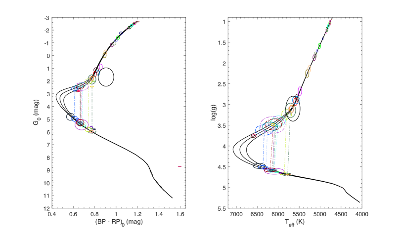
Figure 1 shows the colour-magnitude diagram (CMD) and the temperature-surface gravity diagram for our UMP sample, plotted with three isochrones that cover the age range we considered (). For stars for which the dwarf/giant degeneracy is not broken, we show both solutions connected by a dot-dashed line, where the least probable solution is marked with a dot-dashed ellipse. Only results using a MW halo prior are shown here. As we can see, from the CMD plot (left panel of Figure 1), the method overall works well, except for the HE 0330+0148 ( mag) that lays outside the colour range of the available set of isochrones. This special case is discussed in more detail in section A.13. The distances and stellar parameters lead to the conclusion that 18 stars () are in the main sequence phase, and the other 24 are in the subgiant/giant phase (). This is of course a result of the observing strategies of the multiple surveys that led to the discovery of these stars.
For all 42 stars in our sample, we show the results of our analysis in Figures 4 to 45. In all figures, the top-left panel shows the distance likelihood functions and posterior PDFs, the top-middle panel presents the log(g) PDF, while the top-right panel shows the effective temperature PDF. The orbit of the star in Galactic cartesian coordinates is presented in the bottom panels of the figures.
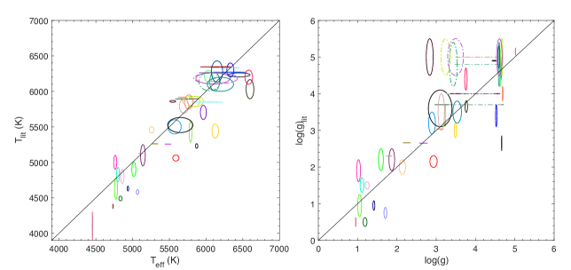
In the subsections of Appendix A, we discuss in detail the results for every star in the sample sorted by right ascension. Specifically, we focus on the inferred distances, stellar parameters, and orbits using a MW halo prior and, when it yields different results, we also discuss the use of the dischalo prior. A global comparison between the inferred stellar parameters form our work and the values from literature is described in Appendix B and shown in the two panels of Figure 46.
We did a comparison between the distances inferred in this work and the ones inferred by Bailer-Jones et al. (2018). These authors use a posterior probability composed by the astrometric likelihood shown in Equation (8) and a MW prior that is based on a Gaia-observed Galaxy distribution function accurately describing the overall distribution of all MW stars. This is naturally more biased to higher densities in the thin disc and thus results in closer distances for most of the stars.
Frebel et al. (2018) compiled a list of 29 UMP stars inferring orbital parameters starting from the MW prior described in Bailer-Jones et al. (2018) but fixing the length-scale parameter to . As both the initial assumptions and the focus of the analysis given in Frebel et al. (2018) significantly differ from the approach taken in this work, we refrain from a further qualitative comparison.
5 Discussions
Our combined analysis of the Gaia DR2 astrometry and photometry with stellar population models for low metallicity stars allows us to infer the stellar parameters and orbital properties of the 42 known UMP stars. We derive well constrained properties for most stars and, in particular, we are now in a position to unravel the possible origin of the heterogeneous sample of UMP stars found to date.
5.1 Insights on the orbits of UMP stars
Apart from 2 ambiguous cases, we can classify the orbits of the UMP stars within three loosely defined categories:
-
•
19 “inner halo” stars, arbitrarily defined as having apocentres smaller than
-
•
12 “outer halo” stars with apocentre larger than
-
•
strikingly, 11 stars that have “MW plane” orbits, by which we mean that they stay confined close to the MW plane ().
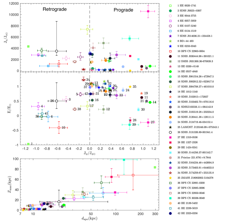
Figure 2 attempts to show these different kind of orbits, displaying on the top panel the vertical component of the action-angle versus the rotational component () for all the UMP in our sample. In this space, the stars confined to the MW plane (denoted by a star marker) are constrained to the lower part of the diagram, while the halo stars have larger . Stars that have a prograde motion have and stars with retrograde orbits lie in the part of the diagram. We note how the Caffau star (SDSS J102915+172927) and 2MASS J18082002-5104378 occupy a special place in this plane and they are the only stars on a quasi-circular orbit at large and low .
It is appealing to assign a tentative origin to stars in these three categories. The “inner halo” stars could well be stars accreted onto the MW during its youth, when its mass was smaller and, therefore, its potential well less deep than it is now. At that time, more energetic orbits would have been unbound and left the MW in formation. “Outer halo” orbits tend to have very radial orbits in this sample (likely a consequence of the window function imparted by the various surveys that discovered these UMP stars; see below), which makes it easier to identify them. It is tempting to see those as being brought in through the accretion of faint dwarf galaxies onto the MW throughout the hierarchical formation of its halo. Although no UMP has been found in MW satellite dwarf galaxies yet, we know of many extremely metal-poor stars in these systems, down to [Fe/H] (e.g., Tafelmeyer et al., 2010) and UMP stars are expected to be present as well (Salvadori, Skúladóttir & Tolstoy, 2015). We note that, among the two “halo” categories, there is a distinct preference for prograde over retrograde orbits.
The 11 “MW plane” orbits are much more unexpected:
-
•
8 stars (SDSS J014036.21+234458.1, BD+44 493, HE 0233-0343, HE 0330+0148, HE 1012-1540, SDSS J103402.70+070116.6, LAMOST J125346.09+075343, SDSS J164234.48+443004.9) share similar rosette orbits within a wide range of angular momentum along the axis (). These stars orbit close to the plane, but not on circular orbits.
- •
-
•
SDSS J174259.67+253135.8 (Figure 37) is retrograde and more likely on an “inner halo” orbit that remains close to the MW plane.
The first ten of those stars, excluding SDSS J174259.67+253135.8, all have positive and thus a prograde orbit, which is unlikely to be a random occurrence ( chance). It is worth noting that it is very unlikely the selection functions that led to the discovery of the UMP stars biased the sample for/against prograde orbit. The origin of those stars is puzzling but we can venture three different hypothesis for their presence in the sample, all of which must account for the fact that this significant fraction of UMP stars, which are expected to be very old, appears to know where the plane of the MW is located, even though the MW plane was unlikely to be in place when they formed.
Scenario 1: The first obvious scenario is that these stars formed in the MW disc itself after the HI disc settled. In this fashion, the stars were born with a quasi-circular orbit and then the presence of a dynamical heating mechanism is mandatory to increase the eccentricity and the height from the plane as a function of time. We find that all the prograde “MW plane” stars and few catalogued as inner halo stars that are confined within and (see Figure 2) overlap in the parameters space (, , , ) with a population of known stars at higher metallicity that Haywood et al. (2018) hypothesise to be born in the thick disc and then dynamical heated by the interaction between the disc and a merging satellite. However, the question is whether in a relatively well-mixed HI disc it is possible to form stars so completely devoid of metals.
Scenario 2: The second scenario is that these stars were brought into the MW by the accretion of a massive satellite dwarf galaxy. Cosmological simulations have shown that merger events are expected to sometimes be aligned with the disc. As a result, significant stellar populations currently in the disc might actually be merger debris (Gómez et al., 2017). Alternatively, Scannapieco et al. (2011), show that 5–20% of disc stars in their simulated MW-like disc galaxies where not formed in situ but, instead, accreted early from now disrupted satellites on co-planar orbits. Additionally, it is well known that the accretion of a massive system onto the MW will see its orbit align with the plane of the MW via dynamical friction, as shown by Abadi et al. (2003) or Peñarrubia, Kroupa & Boily (2002). From these authors’ simulations, one would expect orbits to become such that they would end up with larger eccentricities than the satellite’s orbit at the start of the merging process and also aligned with the disc by dynamical friction and tidal interactions, which is compatible with our orbital inference for the remarkable UMP stars. If such an accretion took place in the MW’s past, it could have brought with it a significant fraction of the UMP stars discovered in the solar neighbourhood. The accretion of the so-called Gaia-Enceladus satellite in the Milky Way’s past (Belokurov et al., 2018; Haywood et al., 2018; Helmi et al., 2018) could be an obvious culprit, however Gaia-Enceladus was discovered via the mainly halo-like and retrograde orbit of its stars whereas the vast majority of the stars we find here are on prograde orbits. In fact, there is no evidence of a particular overdensity of stars in the top-left region of the vs. of Figure 2 where Gaia-Enceladus stars are expected to be found. It would therefore be necessary to summon the presence of another massive or several less massive accretion events onto the MW if this scenario is valid.
Scenario 3: Finally, the third scenario that could explain the presence of this significant fraction of UMP stars that remain confined to the plane of the MW would be one in which these stars originally belonged to one or more of the building blocks of the proto-MW, as it was assembling into the MW that we know today. Fully cosmological simulations confirm that stars that are at the present time deeply embedded in our Galaxy do not need to have their origin in the proto-Galaxy. El-Badry et al. (2018) find in their cosmological simulations that, of all stars formed before presently within of the Galactic centre, less than half were already in the main progenitor at . Over half of these extremely old stars would thus make their way into the main Galaxy in later merging events and find themselves at inside different building blocks that are up to away from the main progenitor centre. In such a scenario, we can expect that whatever gas-rich blocks formed the backbone of the MW disc brought with it its own stars, including UMP stars. Yet, for such a significant number of UMP stars to align with the current MW plane, it is necessary to assume that the formation of the MW’s disc involved a single massive event that imprinted the disc plane that is aligned with the orbit of its stars. The presence of many massive building blocks would have likely led to changes in the angular Hi disc alignment. Similarly, the MW cannot have suffered many massive accretions since high redshift or the disc would have changed its orientation (Scannapieco et al., 2009). This would be in line with expectations that the MW has had an (unusually) quiet accretion history throughout its life (Wyse, 2001; Stewart et al., 2008).
5.1.1 The Caffau star and 2MASS J18082002-5104378
SDSS J102915+172927 (see Figure 22), also known as “the Caffau star” (Caffau et al., 2011), and 2MASS J18082002-5104378 (see Figure 38) both have a disc-like prograde orbit but while the Caffau Star reaches a height of from the MW plane, the latter star is confined within , confirming the results from Schlaufman, Thompson & Casey (2018). Both stars represent outliers inside the surprising sample of “MW planar” stars that typically have more eccentric orbits. For these stars, scenario 3, as outlined above, might be an interesting possibility. A merging between the building blocks of the proto-MW could have brought in these UMP stars and their orbit circularised by dynamical friction.
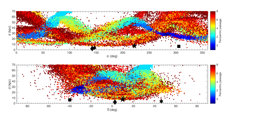
5.1.2 Coincidence with the Sagittarius stream
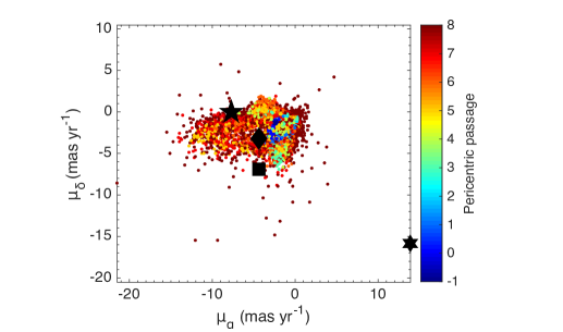
We note that four of the “halo” stars (SDSS J092912.32+023817.0, SDSS J094708.27+461010.0, Pristine221.8781+9.7844 and BPS CS 22885-0096) have orbits that are almost perpendicular to the MW plane (see Figures 19, 20, 34, and 40), coinciding with the plane of the stellar stream left by the Sagittarius (Sgr) dwarf galaxy as it as being tidally disrupted by the MW. We therefore investigate if these stars belong to the stream by comparing their proper motions and distances with the values provided by the N-body simulation of Law & Majewski (2010), hereafter LM10 (see Figure 3). It is clear that SDSS J094708.27+461010.0 has a proper motion that is incompatible with the simulation’s particles. On the other hand, we find that SDSS J092912.32+023817.0, Pristine221.8781+9.7844, and BPS CS 22885-0096 have proper motions that are in broad agreement with those of the simulation. These stars could be compatible with the oldest wraps of the Sgr galaxy but we are nevertheless cautious in this assignment since only the young wraps of the stream were constrained well with observations in the Law & Majewski (2010) model. Older wraps rely on the simulation’s capability to trace the orbit back in the MW potential, that is itself poorly constrained and has likely changed over these timescales, and the true 6D phase-space location the older warps could therefore easily deviate significantly from the simulation’s expectations.
5.1.3 A connection between SDSS J174259.67+253135.8 and Centauri?
SDSS J174259.67+253135.8 is the only star of the “MW planar” sample that has a retrograde motion and its orbital properties are, in fact, similar enough to those of the Centauri (Cen) stellar cluster to hint at a possible connection between the two. It should be noted, however, that the of Cen’s orbit is about twice that of this star. Nevertheless, given the dynamically active life that Cen must have had in the commonly-held scenario that it is the nucleus of a dwarf galaxy accreted by the Milky Way long ago (e.g., Zinnecker et al. 1988; Mizutani, Chiba & Sakamoto 2003), the similarity of the orbits is intriguing enough to warrant further inspection.
5.2 Limits of the analysis and completeness
The heterogeneous UMP sample comes from multiple surveys conducted over the years, with their own, different window functions for the selection of the targets and it can thus by no means be called a complete or homogeneous sample. To reconstruct the full selection function of this sample is nearly impossible since it includes so many inherited window functions from various surveys and follow-up programs. As far as we can deduce, however, none of the programs would have specifically selected stars on particular orbits. We therefore consider the clear preference of the UMP star population for orbits in the plane of the MW disc a strong result of this work but we caution the reader not to consider the ratio of “inner halo,” “outer halo,” and “MW plane” orbits as necessarily representative of the true ratios, which will require a more systematic survey to confirm.
We note that due to the different abundance patterns of these stars, is not always a good tracer of the total metallicity . However, not all stars in this sample are equally well-studied and therefore constraints on are inhomogeneous. This has led us to nevertheless choose a cut on as this is the common quantity measured by all the cited authors.
Another limitation of this work comes from the isochrones we use, which are the most metal-poor isochrones available in the literature at this time and have [Fe/H] dex with solar-scaled -abundances. Beyond the fact that some stars in our sample are significantly more metal-poor than this, not all stars follow this abundance pattern and as a result their total metal-content can change, in turn affecting the colour of the isochrones. We estimate, however, that this will be a small effect at these low metallicities, as low-metallicity isochrones are relatively insensitive to small variations in metallicity, and take this into account adding a systematic uncertainty of 0.01 mag in quadrature to the model (see Section 3.1.1). This is unlikely to affect the final results on the evolutionary phase and the typology of the orbits. A final potential limitation of this work stems from the possible binary of some of the studied stars. If, unbeknownst to us, a star is in fact a binary system whose component are in the same or a similar evolutionary phase, their photometry would not be representative of their true properties and our distant inference would be biased. Similarly a binary star would like have its velocity be affected, leading to flawed orbital parameters. For known binary stars, we nevertheless take these effects into account and our distance and orbital inference should not be severely affected by this binarity issue.
5.3 Future outlook
As described in 5.2, the current sample and analysis of their dynamics is quite limited by an unknown and complicated selection function. With proper motion, parallax, and the exquisite photometry from Gaia DR2, we plan to apply the same bayesian framework described in Section 3 to all the EMP stars within the Pristine survey (Starkenburg et al., 2017a) to investigate their stellar properties and orbits. As the completeness and purity of this sample is very well understood (Youakim et al., 2017) and this sample is much larger, this will open up more quantitative avenues to explore the role of extremely metal-poor stars in the big picture of the accretion history of the MW.
6 Conclusions
Combining the Gaia DR2 photometric and astrometric information in a statistical framework, we determine the posterior probability distribution function for the distance, the stellar parameters (temperature and surface gravity), and the orbital parameters of 42 UMPs (see Tables 3 and 6). Given that 11 of those stars remain confined close to the MW plane, we use both a pure halo prior and a combined dischalo prior. Folding together distance posterior and orbital analysis we find that 18 stars are on the main sequence and the other 24 stars are in a more evolved phase (subgiant or giant).
Through the orbital analysis, we find that 11 stars are orbiting in the plane of disc, with maximum height above the disc within 3 kpc. We hypothesise that they could have once belonged to a massive building blocks of the proto-MW that formed the backbone of the MW disc, or that they were brought into the MW via a specific, massive hierarchical accretion event, or they might have formed in the early disc and have been dynamically heated. Another 31 stars are from both the “inner halo” (arbitrarily defined as having ) and were accreted early on in the history of the MW, or the “outer halo” hinting that they were accreted onto the Galaxy from now-defunct dwarf galaxies. Of these halo stars, SDSS J092912.32+023817.0, Pristine221.8781+9.7844 and BPS CS 22885-0096, could possibly be associated with the Sagittarius stream, although they would need to have been stripped during old pericentric passages of the dwarf galaxy. SDSS J174259.67+253135.8 could also possibly be associated with Cen as its progenitor.
The work presented here provides distances, stellar parameters, and orbits for all known UMP stars and, hence, some of the oldest stars known. To understand their position and kinematics within the Galaxy it is very important to reconstruct the early formation of the MW and/or the hierarchical formation of some of its components. We foresee a statistical improvement of this first study with the arrival of homogeneous and large datasets of EMP stars, such as observed within the Pristine or SkyMapper surveys (Starkenburg et al., 2017a; Wolf et al., 2018). With these surveys, the window function and the selection criteria of the objects for which distances and orbits are derived will be much better known.
Acknowledgements
We would like to thank Benoit Famaey, Misha Haywood and Paola Di Matteo for the insightful discussions and comments.
FS, NFM, NL, and RI gratefully acknowledge funding from CNRS/INSU through the Programme National Galaxies et Cosmologie and through the CNRS grant PICS07708. FS thanks the Initiative dExcellence IdEx from the University of Strasbourg and the Programme Doctoral International PDI for funding his PhD. This work has been published under the framework of the IdEx Unistra and benefits from a funding from the state managed by the French National Research Agency as part of the investments for the future program. ES and AA gratefully acknowledge funding by the Emmy Noether program from the Deutsche Forschungsgemeinschaft (DFG). JIGH acknowledges financial support from the Spanish Ministry project MINECO AYA2017-86389-P, and from the Spanish MINECO under the 2013 Ramón y Cajal program MINECO RYC-2013-14875. KAV thanks NSERC for research funding through the Discovery Grants program.
This research has made use of use of the SIMBAD database, operated at CDS, Strasbourg, France (Wenger et al., 2000). This work has made use of data from the European Space Agency (ESA) mission Gaia (https://www.cosmos.esa.int/gaia), processed by the Gaia Data Processing and Analysis Consortium (DPAC, https://www.cosmos.esa.int/web/gaia/dpac/consortium). Funding for the DPAC has been provided by national institutions, in particular the institutions participating in the Gaia Multilateral Agreement.
| Identifier | [Fe/H] | [C/Fe] | log(g)lit | E(B-V) | Binarity | References | |||||||||
| (deg) | (deg) | (dex) | (dex) | (dex) | (dex) | () | () | (K) | (K) | (dex) | (dex) | (mag) | |||
| HE 0020-1741 | 5.6869167 | 1.4 | 93.06 | 0.83 | 4630.0 | 150 | 0.95 | 0.3 | 0.021 | N | Placco et al. (2016) | ||||
| SDSS J0023+0307 | 5.80834363858 | 3.13284420892 | 1.0 | 6140 | 132 | 4.8 | 0.6 | 0.028 | N | Aguado et al. (2018a) | |||||
| HE 0044-3755 | 11.6508144643 | 48.3 | 2.5 | 4800 | 100 | 1.5 | 0.1 | 0.010 | N | Cayrel et al. (2004) | |||||
| HE 0057-5959 | 14.9749409617 | 0.86 | 375.64a | 1 | 5257 | 2.65 | 0.016 | N | Norris et al. (2007), Norris et al. (2013) | ||||||
| HE 0107-5240 | 17.3714810637 | 0.2 | 3.85 | 46.0a | 2.0 | 5100 | 150 | 2.2 | 0.3 | 0.011 | Ya | Christlieb et al. (2004) | |||
| HE 0134-1519 | 24.2724039774 | 0.2 | 1.00 | 0.26 | 244 | 1 | 5500 | 100 | 3.2 | 0.3 | 0.016 | N | Hansen et al. (2015) | ||
| SDSS J014036.21+234458.1 | 25.1509195676 | 23.7495011637 | 0.3 | 1.1 | 0.3 | a | 1 | 5703 | 100 | 4.7 | 0.3 | 0.114 | Ya | Yong et al. (2013) | |
| BD+44 493 | 36.7072451683 | 44.9629239592 | 0.2 | 1.2 | 0.2 | 0.63 | 5430 | 150 | 3.4 | 0.3 | 0.079 | N | Ito et al. (2013) | ||
| HE 0233-0343 | 39.1241380137 | 0.2 | 3.48 | 0.24 | 64 | 1 | 6300 | 100 | 3.4 | 0.3 | 0.022 | N | Hansen et al. (2015) | ||
| BPS CS 22963-0004 | 44.1940476203 | 0.15 | 0.40 | 0.23 | 292.4 | 0.2 | 5060 | 42 | 2.15 | 0.16 | 0.045 | N | Roederer et al. (2014) | ||
| SDSS J030444.98+391021.1 | 46.1874375223 | 39.1725764233 | 0.2 | 0.7 | 87 | 8 | 5859 | 13 | 5.0 | 0.5 | 0.111 | N | Aguado et al. (2017b) | ||
| SMSS J031300.36-670839.3 | 48.2515614545 | 4.5 | 0.2 | 298.5a | 0.5 | 5125 | 2.3 | 0.032 | N | Keller et al. (2014), Nordlander et al. (2017) | |||||
| HE 0330+0148 | 53.158696449 | 1.96666957231 | 0.1 | 2.6 | a | 1 | 4100 | 200 | 5.2 | 0.1 | 0.094 | Y | Plez, Cohen & Meléndez (2005) | ||
| HE 0557-4840 | 89.6636087844 | 0.2 | 1.65 | 211.9 | 0.8 | 4900 | 100 | 2.2 | 0.3 | 0.037 | N | Norris et al. (2007) | |||
| SDSS J081554.26+472947.5 | 123.976115075 | 47.4965559814 | 5.0 | 23 | 6215 | 82 | 4.7 | 0.5 | 0.063 | N | Aguado et al. (2018b) | ||||
| SDSS J092912.32+023817.0 | 142.301366238 | 2.63806158906 | 388.3 | 10.4 | 5894 | 3.7 | 0.053 | Y | Bonifacio et al. (2015), Caffau et al. (2016) | ||||||
| SDSS J094708.27+461010.0 | 146.784471294 | 46.1694746754 | 0.2 | 1.0 | 0.4 | 12 | 5858 | 73 | 5.0 | 0.5 | 0.013 | N | Aguado et al. (2017a) | ||
| HE 1012-1540 | 153.722814524 | 0.16 | 2.2 | 225.8a | 0.5 | 5230 | 32 | 2.65 | 0.2 | 0.061 | N | Roederer et al. (2014) | |||
| SDSS J102915+172927 | 157.313121378 | 17.4910907404 | 0.06 | 0.7 | 4 | 5850 | 100 | 4.0 | 0.2 | 0.023 | N | Caffau et al. (2011) | |||
| SDSS J103402.70+070116.6 | 158.511301205 | 7.02129528322 | 0.14 | 153 | 3 | 6270 | 0.02 | N | Bonifacio et al. (2018) | ||||||
| SDSS J103556.11+064143.9 | 158.983818359 | 6.6955582264 | 3.08 | 6 | 6262 | 4 | 0.024 | N | Bonifacio et al. (2015) | ||||||
| SDSS J105519.28+232234.0 | 163.830333515 | 23.3761158455 | 0.07 | 0.7 | 62 | 4 | 6232 | 28 | 4.9 | 0.1 | 0.015 | N | Aguado et al. (2017b) | ||
| SDSS J120441.38+120111.5 | 181.172452065 | 12.019865284 | 0.05 | 1.45 | 51 | 3 | 5917 | 3 | 0.024 | N | Placco et al. (2015) | ||||
| SDSS J124719.46-034152.4 | 191.831114232 | 0.18 | 1.61 | 84 | 6 | 6332 | 4 | 0.022 | N | Caffau et al. (2013b) | |||||
| LAMOST J125346.09+075343.1 | 193.44189217 | 7.89526036289 | 0.06 | 1.59 | 78.0 | 0.4 | 6030 | 135 | 3.65 | 0.16 | 0.025 | N | Li et al. (2015) | ||
| SDSS J131326.89-001941.4 | 198.3620349838832 | 0.2 | 2.8 | 0.3 | 268 | 4 | 5525 | 106 | 3.6 | 0.5 | 0.024 | Y | Allende Prieto et al. (2015), | ||
| Frebel et al. (2015), Aguado et al. (2017b) | |||||||||||||||
| HE 1310-0536 | 198.379940261 | 0.2 | 2.36 | 0.23 | 113.2 | 1.7 | 5000 | 100 | 1.9 | 0.3 | 0.037 | N | Hansen et al. (2015) | ||
| HE 1327-2326 | 202.524748159 | 3.78 | 64.4a | 1.3 | 6200 | 100 | 3.7 | 0.3 | 0.066 | N | Frebel et al. (2008) | ||||
| HE 1424-0241 | 216.668044499 | 0.63 | 59.8 | 0.6 | 5260 | 2.66 | 0.055 | N | Norris et al. (2013), Cohen et al. (2008) | ||||||
| SDSS J144256.37-001542.7 | 220.734907425 | 0.21 | 1.59 | 225 | 9 | 5850 | 4 | 0.036 | N | Caffau et al. (2013a) | |||||
| Pristine221.8781+9.7844 | 221.878064787 | 9.78436859397 | 0.13 | 1.76 | 149.0 | 0.5 | 5792 | 100 | 3.5 | 0.5 | 0.020 | N | Starkenburg et al. (2018) | ||
| SDSS J164234.48+443004.9 | 250.643694345 | 44.5013644484 | 0.2 | 0.55 | 0.0 | 4 | 6280 | 150 | 5.0 | 0.3 | 0.011 | N | Aguado et al. (2016) | ||
| SDSS J173403.91+644633.0 | 263.516273652 | 64.7758235012 | 0.2 | 3.1 | 0.2 | 13 | 6183 | 78 | 5.0 | 0.5 | 0.028 | N | Aguado et al. (2017a) | ||
| SDSS J174259.67+253135.8 | 265.748669215 | 25.526636261 | 0.07 | 3.6 | 10.0 | 6345 | 4 | 0.055 | N | Bonifacio et al. (2015) | |||||
| 2MASS J18082002-5104378 | 272.083464041 | 0.07 | 5440 | 100 | 3.0 | 0.2 | 0.101 | Y | Meléndez et al. (2016) | ||||||
| Schlaufman, Thompson & Casey (2018) | |||||||||||||||
| BPS CS 22891-0200 | 293.829490257 | 0.15 | 131 | 10 | 4490 | 33 | 0.5 | 0.1 | 0.068 | N | Roederer et al. (2014) | ||||
| BPS CS 22885-0096 | 305.213220651 | 0.07 | 10 | 4580 | 34 | 0.75 | 0.15 | 0.048 | N | Roederer et al. (2014) | |||||
| BPS CS 22950-0046 | 305.368323431 | 0.14 | 111 | 10 | 4380 | 32 | 0.5 | 0.1 | 0.054 | N | Roederer et al. (2014) | ||||
| BPS CS 30336-0049 | 311.348055352 | 0.09 | 0.31 | 0.8 | 4827 | 100 | 1.5 | 0.2 | 0.054 | N | Lai et al. (2008) | ||||
| HE 2139-5432 | 325.676864649 | 105a | 3 | 5457 | 44 | 2.0 | 0.2 | 0.017 | Ya | Norris et al. (2013) | |||||
| HE 2239-5019 | 340.611864594 | 0.2 | 1.7 | 368.7 | 0.5 | 6100 | 100 | 3.5 | 0.3 | 0.010 | N | Hansen et al. (2015) | |||
| HE 2323-0256 | 351.62419731 | 0.15 | a | 0.3 | 4630 | 34 | 0.95 | 0.13 | 0.043 | N | Roederer et al. (2014) |
| Identifier | Gaia id | G0 | BP0 | RP0 | |||||||||||
| (deg) | (deg) | (mag) | (mag) | (mag) | (mag) | (mag) | (mag) | () | () | () | () | () | () | ||
| HE 0020-1741 | 5.68699047782 | -17.40811466246 | 2367173119271988480 | 12.5609 | 0.00017 | 13.0699 | 0.00095 | 11.904 | 0.00055 | 14.424 | 0.064 | 0.043 | 0.1456 | 0.0384 | |
| SDSS J0023+0307 | 5.80835977813 | 3.1327843082 | 2548541852945056896 | 17.5638 | 0.001 | 17.7947 | 0.0074 | 17.1246 | 0.0074 | 3.743 | 0.318 | 0.187 | 0.2697 | 0.1406 | |
| HE 0044-3755 | 11.65089731416 | 5000753194373767424 | 11.6633 | 0.0003 | 12.1427 | 0.0009 | 11.0310 | 0.0009 | 15.234 | 0.061 | 0.041 | 0.2152 | 0.0344 | ||
| HE 0057-5959 | 14.97496136508 | 4903905598859396480 | 15.0507 | 0.0004 | 15.3857 | 0.0025 | 14.5292 | 0.0025 | 2.389 | 0.042 | 0.041 | 0.1982 | 0.0254 | ||
| HE 0107-5240 | 17.37149810186 | 4927204800008334464 | 14.9334 | 0.0003 | 15.3232 | 0.0019 | 14.3638 | 0.0019 | 2.414 | 0.033 | 0.035 | 0.0789 | 0.0258 | ||
| HE 0134-1519 | 24.27251527664 | 2453397508316944128 | 14.227 | 0.0003 | 14.5501 | 0.0022 | 13.7181 | 0.0022 | 24.961 | 0.056 | 0.039 | 0.3454 | 0.0299 | ||
| SDSS J014036.21+234458.1 | 25.15092436121 | 23.74940873996 | 290930261314166528 | 15.0495 | 0.0006 | 15.3423 | 0.0034 | 14.575 | 0.0034 | 1.019 | 0.176 | 0.091 | 1.0482 | 0.0562 | |
| BD+44 493 | 36.70796538815 | 44.96278519908 | 341511064663637376 | 8.6424 | 0.0005 | 8.9634 | 0.0016 | 8.1758 | 0.0016 | 118.359 | 0.141 | 0.105 | 4.7595 | 0.0660 | |
| HE 0233-0343 | 39.12435352835 | 2495327693479473408 | 15.2126 | 0.0005 | 15.4433 | 0.0027 | 14.8029 | 0.0027 | 49.962 | 0.073 | 0.072 | 0.7925 | 0.0545 | ||
| BPS CS 22963-0004 | 44.1941414394 | 5184426749232471808 | 14.6906 | 0.0005 | 14.9991 | 0.0024 | 14.1973 | 0.0024 | 21.712 | 0.058 | 0.059 | 0.2220 | 0.0364 | ||
| SDSS J030444.98+391021.1 | 46.18743595787 | 39.17249343121 | 142874251765330944 | 17.0085 | 0.0019 | 17.3215 | 0.0088 | 16.5085 | 0.0088 | 0.336 | 0.241 | 0.0752 | 0.1929 | ||
| SMSS J031300.36-670839.3 | 48.25163934361 | 4671418400651900544 | 14.4342 | 0.0003 | 14.8379 | 0.0018 | 13.8545 | 0.0018 | 7.027 | 0.032 | 1.088 | 0.03 | 0.0981 | 0.0162 | |
| HE 0330+0148 | 53.15953261866 | 1.96344241611 | 3265069670684495744 | 13.0859 | 0.0004 | 13.8664 | 0.0032 | 12.2728 | 0.0032 | 194.093 | 0.453 | 0.499 | 12.7174 | 0.2106 | |
| HE 0557-4840 | 89.66361346726 | 4794791782906532608 | 15.0976 | 0.0004 | 15.5156 | 0.0028 | 14.4984 | 0.0028 | 0.718 | 0.043 | 0.735 | 0.044 | 0.0389 | 0.0207 | |
| SDSS J081554.26+472947.5 | 123.97602487635 | 47.49645166114 | 931227322991970560 | 16.5417 | 0.0006 | 16.8056 | 0.0057 | 16.1052 | 0.0057 | 0.135 | 0.09 | 0.4441 | 0.0837 | ||
| SDSS J092912.32+023817.0 | 142.30134736257 | 2.63804791153 | 3844818546870217728 | 17.8302 | 0.0023 | 18.136 | 0.0316 | 17.3618 | 0.0316 | 0.342 | 0.364 | 0.1276 | 0.1872 | ||
| SDSS J094708.27+461010.0 | 146.78455769932 | 46.16940656739 | 821637654725909760 | 18.7343 | 0.0021 | 19.0195 | 0.0221 | 18.2783 | 0.0221 | 13.898 | 0.317 | 0.332 | 0.1989 | 0.2299 | |
| HE 1012-1540 | 153.7223563828 | 3751852536639575808 | 13.7019 | 0.0004 | 14.0084 | 0.0033 | 13.2135 | 0.0033 | 0.046 | 28.13 | 0.04 | 2.5417 | 0.0280 | ||
| SDSS J102915+172927 | 157.31307233934 | 17.49107327845 | 3890626773968983296 | 16.4857 | 0.0013 | 16.7665 | 0.0062 | 15.9976 | 0.0062 | 0.146 | 0.113 | 0.7337 | 0.0780 | ||
| SDSS J103402.70+070116.6 | 158.51126738928 | 7.02126631404 | 3862721340654330112 | 17.1906 | 0.0018 | 17.4051 | 0.0227 | 16.7943 | 0.0063 | 0.236 | 0.291 | 0.2874 | 0.1367 | ||
| SDSS J103556.11+064143.9 | 158.98383317025 | 6.69554785085 | 3862507691800855040 | 18.3472 | 0.0034 | 18.623 | 0.0197 | 17.9584 | 0.0197 | 3.416 | 0.403 | 0.369 | 0.3163 | ||
| SDSS J105519.28+232234.0 | 163.83036912138 | 23.37606935407 | 3989873022818570240 | 17.5182 | 0.0025 | 17.7015 | 0.0317 | 17.1298 | 0.0317 | 7.591 | 0.291 | 0.324 | 0.5909 | 0.1821 | |
| SDSS J120441.38+120111.5 | 181.17245380263 | 12.01984412118 | 3919025342543602176 | 16.027 | 0.0005 | 16.3239 | 0.0043 | 15.5497 | 0.0043 | 0.395 | 0.11 | 0.067 | 0.2454 | 0.0656 | |
| SDSS J124719.46-034152.4 | 191.83107728926 | 3681866216349964288 | 18.1908 | 0.0016 | 18.3958 | 0.0118 | 17.7716 | 0.0118 | 0.439 | 1.812 | 0.226 | 0.3075 | 0.2098 | ||
| LAMOST J125346.09+075343.1 | 193.44198364753 | 7.895007511 | 3733768078624022016 | 12.228 | 0.0002 | 12.4603 | 0.0011 | 11.8239 | 0.0011 | 21.045 | 0.082 | 0.049 | 1.4053 | 0.0378 | |
| SDSS J131326.89-001941.4 | 198.36201866349555 | 3687441358777986688 | 16.3560 | 0.0010 | 16.7237 | 0.0058 | 15.8183 | 0.0710 | 0.160 | 0.078 | 0.2976 | 0.0972 | |||
| HE 1310-0536 | 198.37991838382 | 3635533208672382592 | 14.0256 | 0.0004 | 14.5363 | 0.0021 | 13.3649 | 0.0021 | 0.053 | 0.042 | 0.0078 | 0.0342 | |||
| HE 1327-2326 | 202.52450119109 | 6194815228636688768 | 13.2115 | 0.0004 | 13.45 | 0.0019 | 12.8012 | 0.0019 | 0.04 | 45.498 | 0.035 | 0.8879 | 0.0235 | ||
| HE 1424-0241 | 216.66802803117 | 3643332182086977792 | 15.0437 | 0.0007 | 15.3934 | 0.0046 | 14.5017 | 0.0046 | 0.087 | 0.066 | 0.1152 | 0.0469 | |||
| SDSS J144256.37-001542.7 | 220.73490626598 | 3651420563283262208 | 17.5635 | 0.0023 | 17.8216 | 0.0277 | 17.1364 | 0.0277 | 0.315 | 6.743 | 0.396 | 0.2981 | |||
| Pristine221.8781+9.7844 | 221.87803086877 | 9.78436834556 | 1174522686140620672 | 16.1846 | 0.0009 | 16.4688 | 0.0053 | 15.706 | 0.0053 | 0.110 | 0.116 | 0.1187 | 0.0940 | ||
| SDSS J164234.48+443004.9 | 250.643641407 | 44.50138608236 | 1405755062407483520 | 17.4658 | 0.0012 | 17.6987 | 0.0112 | 17.0356 | 0.0112 | 0.149 | 5.025 | 0.244 | 0.3122 | 0.0906 | |
| SDSS J173403.91+644633.0 | 263.51630029934 | 64.77581642801 | 1632736765377141632 | 19.1198 | 0.0038 | 19.3849 | 0.0465 | 18.7074 | 0.0465 | 2.638 | 0.44 | 0.553 | 0.2702 | ||
| SDSS J174259.67+253135.8 | 265.74864014534 | 25.52658646063 | 4581822389265279232 | 18.5115 | 0.0022 | 18.7628 | 0.0248 | 18.0991 | 0.0248 | 0.248 | 0.292 | 0.1870 | |||
| 2MASS J18082002-5104378 | 272.08342547713 | 6702907209758894848 | 11.488 | 0.0003 | 11.7853 | 0.0024 | 11.0119 | 0.0024 | 0.068 | 0.058 | 1.6775 | 0.0397 | |||
| BPS CS 22891-0200 | 293.82944462026 | 6445220927325014016 | 13.4478 | 0.0003 | 13.9306 | 0.0017 | 12.8053 | 0.0017 | 0.053 | 0.754 | 0.036 | 0.1135 | 0.0342 | ||
| BPS CS 22885-0096 | 305.21319576813 | 6692925538259931136 | 12.9385 | 0.0003 | 13.3482 | 0.0017 | 12.3514 | 0.0017 | 0.038 | 0.028 | 0.1708 | 0.0247 | |||
| BPS CS 22950-0046 | 305.36833037469 | 6876806419780834048 | 13.7403 | 0.0002 | 14.2631 | 0.0011 | 13.0627 | 0.0011 | 1.57 | 0.045 | 0.028 | 0.0587 | 0.0270 | ||
| BPS CS 30336-0049 | 311.34804708033 | 6795730493933072128 | 13.5803 | 0.0002 | 14.074 | 0.0013 | 12.9283 | 0.0013 | 0.038 | 0.027 | 0.0418 | 0.0227 | |||
| HE 2139-5432 | 325.676883449 | 6461736966363075200 | 14.9386 | 0.0003 | 15.2991 | 0.0017 | 14.4 | 0.0017 | 2.547 | 0.046 | 0.041 | 0.0298 | |||
| HE 2239-5019 | 340.61191653735 | 6513870718215626112 | 15.6038 | 0.0007 | 15.8336 | 0.0034 | 15.2107 | 0.0034 | 7.744 | 0.054 | 0.076 | 0.2200 | 0.0545 | ||
| HE 2323-0256 | 351.6242048175 | 2634585342263017984 | 13.9922 | 0.0004 | 14.4286 | 0.0031 | 13.3832 | 0.0031 | 1.742 | 0.062 | 0.048 | 0.0038 | 0.0359 |
| Identifier | D | Teff | log(g) | Area | Prior | |||
| () | () | (K) | (K) | (dex) | (dex) | |||
| HE 0020-1741 | 10.3 | 0.4 | 4774 | 20 | 1.05 | 0.05 | H | |
| 10.3 | 0.4 | 4774 | 20 | 1.05 | 0.05 | DH | ||
| SDSS J0023+0307 | 2.710 | 0.139 | 6116 | 66 | 4.6 | 0.1 | 88% | H |
| 11.03 | 0.73 | 6047 | 146 | 3.4 | 0.1 | 12% | H | |
| 2.693 | 0.136 | 6108 | 65 | 4.6 | 0.1 | 99.6% | DH | |
| 11.02 | 0.74 | 6050 | 154 | 3.4 | 0.1 | 0.4% | DH | |
| HE 0044-3755 | 5.70 | 0.25 | 4852 | 22 | 1.2 | 0.1 | H | |
| 5.65 | 0.26 | 4863 | 23 | 1.2 | 0.1 | DH | ||
| HE 0057-5959 | 6.80 | 0.71 | 5483 | 42 | 2.7 | 0.1 | H | |
| 6.50 | 0.72 | 5501 | 44 | 2.7 | 0.1 | DH | ||
| HE 0107-5240 | 14.3 | 1.0 | 5141 | 32 | 1.9 | 0.1 | H | |
| 14.2 | 1.0 | 5141 | 32 | 1.9 | 0.1 | DH | ||
| HE 0134-1519 | 3.75 | 0.33 | 5572 | 90 | 2.9 | 0.1 | H | |
| 3.61 | 0.30 | 5589 | 37 | 2.9 | 0.1 | DH | ||
| SDSS J014036.21+234458.1 | 0.762 | 0.022 | 5963 | 41 | 4.6 | 0.1 | H | |
| 0.761 | 0.022 | 5962 | 40 | 4.6 | 0.1 | DH | ||
| BD+44 493 | 0.211 | 0.003 | 5789 | 19 | 3.2 | 0.1 | H | |
| 0.211 | 0.003 | 5794 | 20 | 3.2 | 0.1 | DH | ||
| HE 0233-0343 | 1.090 | 0.043 | 6331 | 47 | 4.5 | 0.1 | H | |
| 1.088 | 0.043 | 6327 | 47 | 4.5 | 0.1 | DH | ||
| BPS CS 22963-0004 | 4.47 | 0.42 | 5589 | 42 | 2.9 | 0.1 | H | |
| 4.36 | 0.39 | 5601 | 43 | 3.0 | 0.1 | DH | ||
| SDSS J030444.98+391021.1 | 14.9 | 1.3 | 5547 | 39 | 2.8 | 0.1 | 99% | H |
| 1.505 | 0.071 | 5649 | 68 | 4.7 | 0.1 | 1% | H | |
| 14.3 | 2.5 | 5548 | 74 | 2.8 | 0.2 | 79% | DH | |
| 1.503 | 0.071 | 5648 | 68 | 4.7 | 0.1 | 21% | DH | |
| SMSS J031300.36-670839.3 | 12.0 | 0.8 | 5111 | 31 | 1.8 | 0.1 | H | |
| 12.1 | 0.8 | 5111 | 32 | 1.8 | 0.1 | DH | ||
| HE 0330+0148 | 0.075 | 0.001 | 4454 | 1 | 5.0 | 0.1 | H | |
| 0.075 | 0.001 | 4460 | 1 | 5.0 | 0.1 | DH | ||
| HE 0557-4840 | 20.0 | 1.3 | 5017 | 28 | 1.6 | 0.1 | H | |
| 20.0 | 1.3 | 5018 | 30 | 1.6 | 0.1 | DH | ||
| SDSS J081554.26+472947.5 | 1.591 | 0.067 | 6034 | 56 | 4.6 | 0.1 | H | |
| 1.588 | 0.066 | 6031 | 56 | 4.6 | 0.1 | DH | ||
| SDSS J092912.32+023817.0 | 15.6 | 2.6 | 5708 | 124 | 3.1 | 0.2 | 68% | H |
| 2.398 | 0.205 | 5775 | 122 | 4.7 | 0.1 | 32% | H | |
| 2.367 | 0.198 | 5756 | 120 | 4.7 | 0.1 | 95% | DH | |
| 15.5 | 2.6 | 5713 | 125 | 3.1 | 0.2 | 5% | DH | |
| SDSS J094708.27+461010.0 | 3.84 | 0.30 | 5854 | 110 | 4.7 | 0.1 | 82% | H |
| 21.9 | 2.0 | 5801 | 118 | 3.2 | 0.1 | 18% | H | |
| 3.76 | 0.28 | 5823 | 55 | 4.7 | 0.1 | 98% | DH | |
| 21.9 | 2.0 | 5802 | 120 | 3.2 | 0.1 | 2% | DH | |
| HE 1012-1540 | 0.384 | 0.004 | 5872 | 16 | 4.7 | 0.1 | H | |
| 0.384 | 0.004 | 5870 | 16 | 4.7 | 0.1 | DH | ||
| SDSS J102915+172927 | 1.281 | 0.051 | 5764 | 57 | 4.7 | 0.1 | H | |
| 1.278 | 0.050 | 5761 | 56 | 4.7 | 0.1 | DH |
from previous page. Identifier D Teff log(g) Area Prior () () (K) (K) (dex) (dex) SDSS J103402.70+070116.6 2.79 0.26 6366 110 4.5 0.1 89% H 8.28 0.64 6333 211 3.6 0.1 11% H 2.75 0.25 6330 110 4.5 0.1 99.4% DH 8.18 0.65 6320 200 3.6 0.1 0.6% DH SDSS J103556.11+064143.9 3.97 0.35 6144 110 4.6 0.1 67% H 15.6 1.2 6072 168 3.5 0.1 33% H 3.88 0.32 6114 106 4.6 0.1 95.5% DH 15.6 1.2 6073 175 3.5 0.1 0.5% DH SDSS J105519.28+232234.0 3.49 0.45 6452 147 4.5 0.1 96% H 8.84 0.94 6581 248 3.8 0.2 4% H 3.30 0.39 6387 138 4.5 0.1 99.7% DH 8.79 0.99 6606 257 3.8 0.2 0.3% DH SDSS J120441.38+120111.5 7.03 0.54 5679 56 3.1 0.1 H 6.96 0.53 5686 59 3.1 0.1 DH SDSS J124719.46-034152.4 4.17 0.32 6296 92 4.5 0.1 92% H 13.5 1.0 6256 196 3.6 0.1 8% H 4.09 0.30 6273 90 4.5 0.1 99% DH 13.4 1.0 6263 205 3.6 0.1 1% DH LAMOST J125346.09+075343.1 0.766 0.016 6598 52 3.8 0.1 H 0.766 0.016 6608 52 3.8 0.1 DH SDSS J131326.89-001941.4 8.59 2.86 5649 171 3.1 0.3 99.96% H 1.765 0.248 6278 171 4.5 0.1 0.04% H 8.07 2.70 5687 185 3.1 0.3 96.85% DH 1.707 0.227 6237 164 4.6 0.1 3.15% DH HE 1310-0536 20.6 0.9 4788 20 1.0 0.1 H 20.6 0.9 4764 21 1.0 0.1 DH HE 1327-2326 1.212 0.024 6581 52 3.8 0.1 H 1.212 0.024 6591 51 3.8 0.1 DH HE 1424-0241 10.3 1.0 5308 40 2.3 0.1 H 10.3 1.0 5308 40 2.3 0.1 DH SDSS J144256.37-001542.7 11.3 1.0 5993 165 3.4 0.1 87% H 2.683 0.266 6104 128 4.6 0.1 13% H 2.634 0.249 6079 124 4.6 0.1 84% DH 11.3 1.0 5998 172 3.4 0.1 16% DH Pristine221.8781+9.7844 7.36 0.55 5700 63 3.1 0.1 H 7.28 0.52 5710 65 3.1 0.1 DH SDSS J164234.48+443004.9 2.66 0.16 6149 77 4.6 0.1 99% H 10.2 0.7 6126 163 3.5 0.1 1% H 2.64 0.16 6140 76 4.6 0.1 99.95% DH 10.1 0.7 6148 172 3.5 0.1 0.05% DH SDSS J173403.91+644633.0 5.46 1.02 6094 233 4.6 0.1 86% H 21.8 3.0 6131 297 3.5 0.2 14% H 5.05 0.79 5992 208 4.6 0.1 97% DH 21.7 3.0 6134 302 3.5 0.2 3% DH SDSS J174259.67+253135.8 4.46 0.52 6194 145 4.6 0.1 63% H 16.6 1.4 6115 198 3.5 0.1 37% H 4.34 0.48 6162 140 4.6 0.1 94% DH 16.5 1.4 6118 206 3.5 0.1 6% DH 2MASS J18082002-5104378 0.647 0.012 6124 44 3.5 0.1 H 0.647 0.012 6133 44 3.5 0.1 DH BPS CS 22891-0200 14.7 0.5 4789 2 1.2 0.1 H 13.6 0.6 4836 22 1.2 0.1 DH
from previous page. Identifier D Teff log(g) Area Prior () () (K) (K) (dex) (dex) BPS CS 22885-0096 6.65 0.22 5068 16 1.7 0.1 H 6.61 0.38 5070 27 1.7 0.1 DH BPS CS 22950-0046 19.1 0.3 4780 1.0 H 19.1 0.3 4780 1.0 DH BPS CS 30336-0049 15.5 0.7 4809 20 1.1 0.1 H 15.5 0.7 4802 21 1.1 0.1 DH HE 2139-5432 11.0 0.9 5259 34 2.1 0.1 H 11.0 0.9 5259 34 2.1 0.1 DH HE 2239-5019 4.19 0.28 6195 179 3.5 0.1 H 4.13 0.16 6411 100 3.6 0.1 DH HE 2323-0256 14.2 0.6 4937 22 1.4 0.1 H 14.2 0.6 4937 22 1.4 0.1 DH
| Identifier | X | Y | Z | U | V | W | Apo | Peri | Lz | E | Orbit | |
| () | () | () | () | () | () | () | () | () | (km2 s-2) | |||
| HE 0020-1741 | 7.909 | 1.84 | -8.846 | -428.7 | -446.4 | -192.2 | 295.8 | 12.0 | 0.92 | -2311.5 | 63046.1 | IH |
| SDSS J0023+0307 | 8.456 | 1.311 | -2.375 | 76.8 | -251.2 | 69.2 | 9.8 | 0.6 | 0.88 | 108.2 | -68950.0 | IH |
| NB | NB | NB | NB | NB | NB | NB | NB | NB | NB | NB | NB | |
| HE 0044-3755 | 7.353 | -0.824 | -5.61 | -235.9 | -397.1 | -18.1 | 21.8 | 4.5 | 0.66 | -885.7 | -35273.2 | IH |
| HE 0057-5959 | 6.077 | -3.206 | -5.839 | 206.5 | -456.5 | -129.0 | 31.3 | 9.0 | 0.56 | -1947.5 | -20642.9 | OH |
| HE 0107-5240 | 5.255 | -5.497 | -12.877 | 12.5 | -294.3 | 77.2 | 15.9 | 3.2 | 0.66 | -354.3 | -46879.6 | IH |
| HE 0134-1519 | 9.025 | 0.244 | -3.679 | -302.5 | -416.8 | -197.1 | 70.2 | 4.1 | 0.87 | -1555.1 | 2196.4 | OH |
| SDSS J014036.21+234458.1 | 8.447 | 0.414 | -0.473 | 132.8 | -153.5 | 61.5 | 11.4 | 2.5 | 0.64 | 884.9 | -61399.9 | P |
| BD+44 493 | 8.157 | 0.131 | -0.054 | 30.6 | -184.5 | 51.8 | 8.3 | 1.5 | 0.69 | 549.6 | -76078.3 | P |
| HE 0233-0343 | 8.62 | 0.063 | -0.913 | -175.5 | -209.8 | 27.5 | 11.9 | 1.0 | 0.85 | 344.6 | -62501.0 | P |
| BPS CS 22963-0004 | 10.739 | -0.087 | -3.62 | -421.8 | -359.1 | -39.2 | 155.8 | 3.0 | 0.96 | -1134.0 | 25397.6 | OH |
| SDSS J030444.98+391021.1 | NB | NB | NB | NB | NB | NB | NB | NB | NB | NB | NB | NB |
| 9.24 | 0.735 | -0.435 | -77.0 | -33.8 | -139.9 | 16.5 | 7.9 | 0.35 | 1960.2 | -40260.6 | IH | |
| SMSS J031300.36-670839.3 | 5.821 | -8.413 | -8.566 | -218.6 | -459.4 | -32.7 | 40.4 | 5.8 | 0.76 | 519.6 | -14038.7 | OH |
| HE 0330+0148 | 8.055 | -0.003 | -0.049 | 106.0 | -240.9 | -71.1 | 9.0 | 0.5 | 0.89 | 83.2 | -72495.6 | P |
| HE 0557-4840 | 12.281 | -17.142 | -9.58 | -110.0 | -203.0 | -32.5 | 23.4 | 8.2 | 0.48 | 2273.1 | -29646.0 | IH |
| SDSS J081554.26+472947.5 | 9.332 | 0.185 | 0.892 | -12.2 | -176.1 | -156.2 | 9.7 | 5.0 | 0.32 | 705.3 | -59940.5 | IH |
| SDSS J092912.32+023817.0 | 9.225 | -1.502 | 1.401 | -218.9 | -275.2 | 178.3 | 23.5 | 2.7 | 0.79 | 91.4 | -33988.5 | IH/S |
| 16.138 | -9.971 | 9.303 | -321.7 | -447.3 | -102.6 | 193.7 | 21.1 | 0.8 | -51.8 | 34372.9 | OH | |
| SDSS J094708.27+461010.0 | 10.521 | 0.326 | 2.941 | 205.0 | -264.7 | 197.6 | 30.0 | 8.2 | 0.58 | -71.0 | -21786.8 | OH |
| NB | NB | NB | NB | NB | NB | NB | NB | NB | NB | NB | NB | |
| HE 1012-1540 | 8.074 | -0.316 | 0.207 | -222.5 | -191.1 | 49.0 | 14.0 | 1.3 | 0.83 | 552.7 | -55562.1 | P |
| SDSS J102915+172927 | 8.537 | -0.481 | 1.062 | -31.1 | -23.7 | -68.7 | 10.9 | 8.6 | 0.12 | 1952.3 | -49546.0 | P |
| SDSS J103402.70+070116.6 | 8.917 | -1.482 | 2.209 | -97.0 | -178.5 | 35.4 | 10.2 | 2.3 | 0.63 | 775.0 | -65816.8 | P |
| 10.714 | -4.385 | 6.535 | -188.8 | -366.7 | -126.1 | 24.3 | 9.3 | 0.46 | -426.0 | -27566.6 | IH | |
| SDSSJ103556.11+064143.9 | 9.26 | -2.106 | 3.131 | 87.9 | 2.2 | -20.0 | 22.2 | 7.1 | 0.52 | 2137.3 | -32395.0 | IH |
| 12.915 | -8.218 | 12.216 | 300.8 | -60.8 | 25.1 | 147.8 | 11.9 | 0.86 | -99.4 | 25522.1 | OH | |
| SDSS J105519.28+232234.0 | 9.313 | -0.922 | 3.204 | 155.4 | -150.7 | 90.2 | 15.2 | 4.9 | 0.52 | 790.4 | -45745.3 | IH |
| SDSS J120441.38+120111.5 | 8.213 | -2.304 | 6.814 | 92.3 | -149.9 | 6.2 | 12.8 | 3.7 | 0.55 | 597.9 | -53841.3 | IH |
| SDSS J124719.46-034152.4 | 6.874 | -1.879 | 3.581 | -141.4 | -102.9 | 88.2 | 9.9 | 5.0 | 0.41 | 1263.5 | -55819.2 | IH |
| NB | NB | NB | NB | NB | NB | NB | NB | NB | NB | NB | NB | |
| LAMOST J125346.09+075343.1 | 7.856 | -0.208 | 0.723 | 188.3 | -148.3 | 2.6 | 13.4 | 1.9 | 0.75 | 766.8 | -56611.4 | P |
| SDSS J131326.89-001941.4 | 4.472 | -3.561 | 9.327 | 92.1 | -443.7 | 99.5 | 20.4 | 8.5 | 0.41 | -1256.6 | -34000.2 | IH |
| HE 1310-0536 | 0.259 | -8.32 | 17.184 | -284.9 | -448.9 | 47.0 | 99.7 | 19.0 | 0.68 | 2216.2 | 15227.9 | OH |
| HE 1327-2326 | 7.332 | -0.686 | 0.755 | -279.3 | -68.7 | 287.8 | 91.4 | 7.4 | 0.85 | 1522.3 | 11193.7 | OH |
| HE 1424-0241 | 1.915 | -1.738 | 8.108 | -26.0 | -233.7 | 44.9 | 8.8 | 0.9 | 0.81 | 58.6 | -71087.9 | IH |
from previous page. Identifier X Y Z U V W Apo Peri Lz E Orbit (kpc) (kpc) (kpc) () () () (kpc) (kpc) () (km2 s-2) SDSS J144256.37-001542.7 NB NB NB NB NB NB NB NB NB NB NB NB 6.366 -0.233 2.033 93.2 42.0 217.1 39.1 6.7 0.71 1832.0 -14290.8 OH Pristine 221.8781+9.7844 3.941 0.432 6.4 -249.6 -194.4 -6.7 14.1 4.9 0.49 123.6 -47818.2 IH/S SDSS J164234.48+443004.9 7.283 1.869 1.742 -124.6 -143.0 -6.7 9.2 1.6 0.72 539.8 -70959.7 P SDSS J173403.91+644633.0 8.374 4.823 3.089 66.2 -174.4 -200.0 13.0 7.7 0.33 980.4 -43731.4 IH NB NB NB NB NB NB NB NB NB NB NB NB SDSS J174259.67+253135.8 5.293 3.185 2.0 74.6 -348.1 -58.7 8.0 1.0 0.77 -227.0 -78634.3 IH//P NB NB NB NB NB NB NB NB NB NB NB NB 2MASS J18082002-5104378 7.40 P BPS CS 22891-0200 -2.803 -5.036 -6.553 255.7 -93.4 222.1 64.0 7.4 0.8 -1788.2 1304.9 OH BPS CS 22885-0096 2.413 0.123 -3.701 -145.0 -241.8 223.8 9.3 3.6 0.44 5.2 -63004.7 IH/S BPS CS 22950-0046 -6.594 8.665 -8.233 59.4 -70.6 -222.9 41.7 2.5 0.89 -572.2 -14149.5 OH BPS CS 30336-0049 -4.037 3.41 -9.176 -31.8 -643.6 119.8 122.7 8.1 0.88 1489.5 19080.8 OH HE 2139-5432 0.746 -2.466 -8.023 -48.5 -264.7 -113.8 9.8 1.1 0.79 87.2 -66571.3 IH HE 2239-5019 5.857 -0.731 -3.406 125.2 -540.5 -248.0 52.9 6.8 0.77 -1792.6 -4551.9 OH HE 2323-0256 6.687 7.11 -11.698 -53.7 -199.4 20.4 15.4 2.8 0.68 44.7 -48598.2 IH
References
- Abadi et al. (2003) Abadi M. G., Navarro J. F., Steinmetz M., Eke V. R., 2003, ApJ, 597, 21
- Abohalima & Frebel (2018) Abohalima A., Frebel A., 2018, ApJSupp, 238, 36
- Aguado et al. (2016) Aguado D. S., Allende Prieto C., González Hernández J. I., Carrera R., Rebolo R., Shetrone M., Lambert D. L., Fernández-Alvar E., 2016, A&A, 593, A10
- Aguado et al. (2018a) Aguado D. S., Allende Prieto C., González Hernández J. I., Rebolo R., 2018a, ApJL, 854, L34
- Aguado et al. (2017a) Aguado D. S., Allende Prieto C., González Hernández J. I., Rebolo R., Caffau E., 2017a, A&A, 604, A9
- Aguado et al. (2017b) Aguado D. S., González Hernández J. I., Allende Prieto C., Rebolo R., 2017b, A&A, 605, A40
- Aguado et al. (2018b) —, 2018b, ApJL, 852, L20
- Allende Prieto et al. (2015) Allende Prieto C. et al., 2015, A&A, 579, A98
- Arentsen et al. (2018) Arentsen A., Starkenburg E., Shetrone M. D., Venn K. A., Depagne É., McConnachie A. W., 2018, arXiv e-prints
- Bailer-Jones (2015) Bailer-Jones C. A. L., 2015, Publications of the Astronomical Society of the Pacific, 127, 994
- Bailer-Jones et al. (2018) Bailer-Jones C. A. L., Rybizki J., Fouesneau M., Mantelet G., Andrae R., 2018, AJ, 156, 58
- Beers & Christlieb (2005) Beers T. C., Christlieb N., 2005, ARAA, 43, 531
- Beers, Preston & Shectman (1985) Beers T. C., Preston G. W., Shectman S. A., 1985, AJ, 90, 2089
- Belokurov et al. (2018) Belokurov V., Erkal D., Evans N. W., Koposov S. E., Deason A. J., 2018, MNRAS, 478, 611
- Binney & Tremaine (2008) Binney J., Tremaine S., 2008, Galactic Dynamics: Second Edition. Princeton University Press
- Bland-Hawthorn & Gerhard (2016) Bland-Hawthorn J., Gerhard O., 2016, ARAA, 54, 529
- Bonifacio et al. (2015) Bonifacio P. et al., 2015, A&A, 579, A28
- Bonifacio et al. (2018) —, 2018, A&A, 612, A65
- Bovy (2015) Bovy J., 2015, ApJSupp, 216, 29
- Caffau et al. (2012) Caffau E. et al., 2012, A&A, 542, A51
- Caffau et al. (2013a) —, 2013a, A&A, 560, A15
- Caffau et al. (2011) Caffau E. et al., 2011, Nature, 477, 67 EP
- Caffau et al. (2013b) Caffau E. et al., 2013b, A&A, 560, A71
- Caffau et al. (2016) —, 2016, A&A, 595, L6
- Cayrel et al. (2004) Cayrel R. et al., 2004, A&A, 416, 1117
- Choi et al. (2016) Choi J., Dotter A., Conroy C., Cantiello M., Paxton B., Johnson B. D., 2016, ApJ, 823, 102
- Christlieb et al. (2004) Christlieb N., Gustafsson B., Korn A. J., Barklem P. S., Beers T. C., Bessell M. S., Karlsson T., Mizuno-Wiedner M., 2004, ApJ, 603, 708
- Christlieb, Wisotzki & Graßhoff (2002) Christlieb N., Wisotzki L., Graßhoff G., 2002, A&A, 391, 397
- Cohen et al. (2008) Cohen J. G., Christlieb N., McWilliam A., Shectman S., Thompson I., Melendez J., Wisotzki L., Reimers D., 2008, ApJ, 672, 320
- Cui et al. (2012) Cui X.-Q. et al., 2012, Research in Astronomy and Astrophysics, 12, 1197
- Dahn et al. (1977) Dahn C. C., Liebert J., Kron R. G., Spinrad H., Hintzen P. M., 1977, ApJ, 216, 757
- Dearborn et al. (1986) Dearborn D. S. P., Liebert J., Aaronson M., Dahn C. C., Harrington R., Mould J., Greenstein J. L., 1986, ApJ, 300, 314
- Dotter (2016) Dotter A., 2016, ApJSupp, 222, 8
- Eisenstein et al. (2011) Eisenstein D. J. et al., 2011, AJ, 142, 72
- El-Badry et al. (2018) El-Badry K. et al., 2018, MNRAS, 480, 652
- Evans et al. (2018) Evans D. W. et al., 2018, A&A, 616, A4
- Frebel et al. (2015) Frebel A., Chiti A., Ji A. P., Jacobson H. R., Placco V. M., 2015, ApJL, 810, L27
- Frebel et al. (2008) Frebel A., Collet R., Eriksson K., Christlieb N., Aoki W., 2008, ApJ, 684, 588
- Frebel et al. (2018) Frebel A., Ji A. P., Ezzeddine R., Hansen T. T., Chiti A., Thompson I. B., Merle T., 2018, ArXiv e-prints
- Frebel & Norris (2015) Frebel A., Norris J. E., 2015, ARAA, 53, 631
- Freeman & Bland-Hawthorn (2002) Freeman K., Bland-Hawthorn J., 2002, ARAA, 40, 487
- Gaia Collaboration et al. (2018) Gaia Collaboration, Brown A. G. A., Vallenari A., Prusti T., de Bruijne J. H. J., Babusiaux C., Bailer-Jones C. A. L., 2018, ArXiv e-prints
- Gaia Collaboration et al. (2016) Gaia Collaboration et al., 2016, A&A, 595, A1
- Gómez et al. (2017) Gómez F. A. et al., 2017, MNRAS, 472, 3722
- Greif (2015) Greif T. H., 2015, Computational Astrophysics and Cosmology, 2, 3
- Hansen et al. (2015) Hansen T. et al., 2015, ApJ, 807, 173
- Haywood et al. (2018) Haywood M., Di Matteo P., Lehnert M. D., Snaith O., Khoperskov S., Gómez A., 2018, ApJ, 863, 113
- Helmi et al. (2018) Helmi A., Babusiaux C., Koppelman H. H., Massari D., Veljanoski J., Brown A. G. A., 2018, Nature, 563, 85
- Hernitschek et al. (2018) Hernitschek N. et al., 2018, The Astrophysical Journal, 859, 31
- Ito et al. (2013) Ito H., Aoki W., Beers T. C., Tominaga N., Honda S., Carollo D., 2013, ApJ, 773, 33
- Karlsson, Bromm & Bland-Hawthorn (2013) Karlsson T., Bromm V., Bland-Hawthorn J., 2013, Reviews of Modern Physics, 85, 809
- Keller et al. (2014) Keller S. C. et al., 2014, Nature, 506, 463 EP
- Lai et al. (2008) Lai D. K., Bolte M., Johnson J. A., Lucatello S., Heger A., Woosley S. E., 2008, ApJ, 681, 1524
- Law & Majewski (2010) Law D. R., Majewski S. R., 2010, ApJ, 714, 229
- Li et al. (2015) Li H., Aoki W., Zhao G., Honda S., Christlieb N., Suda T., 2015, PASJ, 67, 84
- Lindegren et al. (2018) Lindegren L. et al., 2018, A&A, 616, A2
- Marigo et al. (2008) Marigo P., Girardi L., Bressan A., Groenewegen M. A. T., Silva L., Granato G. L., 2008, A&A, 482, 883
- Meléndez et al. (2016) Meléndez J., Placco V. M., Tucci-Maia M., Ramírez I., Li T. S., Perez G., 2016, A&A, 585, L5
- Mizutani, Chiba & Sakamoto (2003) Mizutani A., Chiba M., Sakamoto T., 2003, ApJL, 589, L89
- Navarro, Frenk & White (1997) Navarro J. F., Frenk C. S., White S. D. M., 1997, ApJ, 490, 493
- Nordlander et al. (2017) Nordlander T., Amarsi A. M., Lind K., Asplund M., Barklem P. S., Casey A. R., Collet R., Leenaarts J., 2017, A&A, 597, A6
- Norris et al. (2013) Norris J. E. et al., 2013, ApJ, 762, 25
- Norris et al. (2007) Norris J. E., Christlieb N., Korn A. J., Eriksson K., Bessell M. S., Beers T. C., Wisotzki L., Reimers D., 2007, ApJ, 670, 774
- Paxton et al. (2011) Paxton B., Bildsten L., Dotter A., Herwig F., Lesaffre P., Timmes F., 2011, ApJSupp, 192, 3
- Peñarrubia, Kroupa & Boily (2002) Peñarrubia J., Kroupa P., Boily C. M., 2002, MNRAS, 333, 779
- Placco et al. (2016) Placco V. M. et al., 2016, ApJ, 833, 21
- Placco et al. (2015) Placco V. M., Frebel A., Lee Y. S., Jacobson H. R., Beers T. C., Pena J. M., Chan C., Heger A., 2015, ApJ, 809, 136
- Plez, Cohen & Meléndez (2005) Plez B., Cohen J., Meléndez J., 2005, Proceedings of The International Astronomical Union, 228
- Roederer et al. (2014) Roederer I. U., Preston G. W., Thompson I. B., Shectman S. A., Sneden C., Burley G. S., Kelson D. D., 2014, The Astronomical Journal, 147, 136
- Roeser, Demleitner & Schilbach (2010) Roeser S., Demleitner M., Schilbach E., 2010, AJ, 139, 2440
- Salpeter (1955) Salpeter E. E., 1955, ApJ, 121, 161
- Salvadori, Skúladóttir & Tolstoy (2015) Salvadori S., Skúladóttir Á., Tolstoy E., 2015, MNRAS, 454, 1320
- Scannapieco et al. (2009) Scannapieco C., White S. D. M., Springel V., Tissera P. B., 2009, MNRAS, 396, 696
- Scannapieco et al. (2011) —, 2011, MNRAS, 417, 154
- Schlaufman, Thompson & Casey (2018) Schlaufman K. C., Thompson I. B., Casey A. R., 2018, ApJ, 867, 98
- Schlegel, Finkbeiner & Davis (1998) Schlegel D. J., Finkbeiner D. P., Davis M., 1998, ApJ, 500, 525
- Schönrich, Binney & Dehnen (2010) Schönrich R., Binney J., Dehnen W., 2010, MNRAS, 403, 1829
- Sharma (2017) Sharma S., 2017, ARAA, 55, 213
- Starkenburg et al. (2018) Starkenburg E. et al., 2018, MNRAS, 481, 3838
- Starkenburg et al. (2017a) —, 2017a, MNRAS, 471, 2587
- Starkenburg et al. (2017b) Starkenburg E., Oman K. A., Navarro J. F., Crain R. A., Fattahi A., Frenk C. S., Sawala T., Schaye J., 2017b, MNRAS, 465, 2212
- Stewart et al. (2008) Stewart K. R., Bullock J. S., Wechsler R. H., Maller A. H., Zentner A. R., 2008, ApJ, 683, 597
- Tafelmeyer et al. (2010) Tafelmeyer M. et al., 2010, A&A, 524, A58
- Wenger et al. (2000) Wenger M. et al., 2000, A&ASupp, 143, 9
- Wolf et al. (2018) Wolf C. et al., 2018, PASA, 35, e010
- Wyse (2001) Wyse R. F. G., 2001, in Astronomical Society of the Pacific Conference Series, Vol. 230, Galaxy Disks and Disk Galaxies, Funes J. G., Corsini E. M., eds., pp. 71–80
- Yanny et al. (2009) Yanny B. et al., 2009, AJ, 137, 4377
- Yong et al. (2013) Yong D. et al., 2013, ApJ, 762, 26
- York et al. (2000) York D. G. et al., 2000, AJ, 120, 1579
- Youakim et al. (2017) Youakim K. et al., 2017, MNRAS, 472, 2963
- Zinnecker et al. (1988) Zinnecker H., Keable C. J., Dunlop J. S., Cannon R. D., Griffiths W. K., 1988, in IAU Symposium, Vol. 126, The Harlow-Shapley Symposium on Globular Cluster Systems in Galaxies, Grindlay J. E., Philip A. G. D., eds., p. 603
Appendix A Individual results
A.1 HE 0020-1741
Figure 4 shows our results for HE 0020-1741, an ultra metal-poor star studied by Placco et al. (2016). Even if the parallax from Gaia DR2 has a large uncertainty (; red solid line for the MW halo prior and a red dot-dashed line for the dischalo prior in the top-left pane), it is enough to break the dwarf/giant degeneracy obtained from the photometric solution (black line). The final PDFs are shown, using the MW halo prior and the dischalo prior, respectively as the solid blue and the dot-dashed blue curves in that panel and, in both cases, the final scenario is a giant located at . The stellar parameters we infer are in agreement with the values from the literature. In the lower panels of Figure 4, both the orbits calculated from the inferred distances from the PDF and Gaia astrometry only are shown, respectively marked by the blue and the red lines. The orbital parameters relative to the distance PDF represent an unbound orbit, while the Gaia astrometric distance leads to a more benign orbit that remains in the inner part of the MW halo.
A.2 SDSS J0023+0307
Figure 5 summarises our results for SDSS J0023+0307, which is a mega metal-poor star found by Aguado et al. (2018a). The Gaia parallax is not very informative (; red solid line for the MW halo prior and a red dot-dashed line for the dischalo prior in the top-left panel) and cannot break the dwarf/giant degeneracy inherent to the photometric solution (black line). It is nevertheless entirely compatible with that inference. The final PDFs are shown, using the MW halo prior and the dischalo prior, respectively as the solid blue and the dot-dashed blue curves in that panel and, in both cases, yields a more likely dwarf solution at along with a less likely sub-giant solution at . The stellar parameters we infer for the most likely dwarf solution are entirely compatible with the literature values. Combined with the exquisite Gaia proper motions, the two distance solutions yield drastically different orbits. The sub-giant distance peak implies an unbound orbit that is shown in orange, while the (more likely) dwarf solution produces a more benign orbit that remains within the inner MW (shown in blue), supporting the distance of the latter solution as the valid one. While eccentric, this orbit surprisingly remains confined close to the MW plane ()
A.3 HE 0044-3755
HE 0044-3755 is an ultra metal-poor star studied by Cayrel et al. (2004) and our results for this star are shown in Figure 6. The distance PDF constrains the distance to . This result leads to a giant solution that is compatible with the values in the literature. The orbit of this star is typical of a halo star.
A.4 HE 0057-5959
Our results for HE 0057-5959 are shown in Figure 7, taking the literature values from Norris et al. (2013). From the distance PDF, we see a disagreement between the photometric and the astrometric likelihoods, which we cannot trace to any obvious source, but the astrophysical parameter inference is compatible with the literature values. For this giant, we show the orbit inferred both from our full astrometric and photometric analysis (blue orbit) and when using only the Gaia astrometry with the MW prior (red orbit). In both cases, HE 0057-5959 remains in the inner region of the MW halo (apocentre ).
A.5 HE 0107-5240
HE 0107-5240 is likely a binary system (Arentsen et al., 2018) discovered by radial velocity variation. Its spectrum does not present double lines indicating that the light is not polluted by the secondary. It is a hyper metal-poor star analysed by Christlieb et al. (2004). Our results are shown in Figure 8 and we infer a distance of , corresponding to the giant solution because the probability of the dwarf solution is entirely suppressed by the Gaia parallax information. Our values for surface gravity and effective temperature are in perfect agreement with the literature values. The orbit of this star is typical of an eccentric halo orbit and remains within .
A.6 HE 0134-1519
Our analysis of HE 0134-1519 (Hansen et al., 2015) is shown in Figure 9. This is another case for which the astrometric and photometric likelihoods disagree, yielding very different orbits, even though it is clear this star is a giant, in agreement with the literature. Both orbital solutions are indicative of a halo star, but the closer Gaia-only distance solution yields an orbit that remains much closer to the Galactic center (apocentre of vs. ).
A.7 SDSS J014036.21+234458.1
For the dwarf star SDSS J014036.21+234458.1 (Yong et al., 2013, Figure 10), the astrometric and photometric distances are technically in disagreement, but the distance inferences are so similar that it does not impact our results. We infer a distance of and an orbit that brings SDSS J014036.21+234458.1 close to the MW plane ().
A.8 BD+44 493
A.9 HE 0233-0343
The combined astrometric and photometric analysis of HE 0233-0343 (Hansen et al., 2015, Figure 12) yields an accurate distance of . Despite this, our inference is incompatible with the literature value, but the very accurate Gaia parallax lends support to our inference. Like the previous star, HE 0233-0343 remains confined to the region of the MW disc, with and an apocentre of .
A.10 BPS CS 22963-0004
For this UMP studied by Roederer et al. (2014), we infer a distance of (Figure 13). Our astrophysical parameter inference disagrees with the literature values but the MESA isochrones strongly constrain our temperature inference. The difference could hint at systematics in these isochrones or the Roederer et al. (2014) analysis. Despite the currently proximity to this star, its orbit brings it very far into the MW halo, with .
A.11 SDSS J030444.98+391021.1
The Gaia parallax of SDSS J030444.98+391021.1 (Aguado et al., 2017b, Figure 14) is very uncertain () but, in case of the halo prior, strongly suppresses the dwarf solution (1% of the PDF). However, the orbital analysis shows that the favoured giant scenario implies that this star is not bound to the MW. According to this, we repeat the analysis with the dischalo prior finding that the inferred distances are not significantly changed but the fractional probability of the peaks is. With this prior, the dwarf solution represents 21 of the PDF. Taking into account the orbital analysis, the dwarf solution appears to be the more realistic distance estimate (). This solution is also compatible with the of Aguado et al. (2017b), contrary to the result from the giant solution. We note that a slightly larger distance for the dwarf solution would be entirely compatible with the Gaia parallax and we think that the low likelihood of the dwarf solution could be driven further down than it should by a systematic in the models we use. With our favoured close-by distance, this star has the orbit of an inner halo object.
A.12 SMSS J031300.36-670839.3
For this star with the lowest iron-abundance (, Nordlander et al., 2017, Figure 15), we infer a distance of corresponding to the giant solution (). The literature is however in better agreement with the Gaia-only distance that is a little closer. The orbital analysis implies that this star has a fairly eccentric orbit and that, using the Gaia-only distance, it is compatible with an inner halo object. With the final posterior, we infer an outer halo orbit.
A.13 HE 0330+0148
As we can see in Figure 1, the analysis fails for this carbon-enhanced star (also known as G77-61) and its location in the colour-magnitude diagram does not coincide with the isochrone models. The strong carbon bands dominate in the spectrum (Dahn et al., 1977) , where the Gaia DR2 filter is sensitive, leading to an abnormal value of () colour and, as a consequence, this star lays outside the isochrone range. This could also explain the strong disagreement between the photometric-only and astrometric-only distance likelihood functions (see Figure 16). We don’t think that the binarity can affects the photometry because the companion is most likely an unseen white dwarf with a period of 250 days (Dearborn et al., 1986), which means that the Gaia DR2 magnitudes correspond to the magnitude of the star itself and not that of the binary system. In this case, we favour the Gaia-only inference with . HE 0330+0148 has a very radial orbit and its current position near the Sun is near its apocentre. Its orbit is close to the MW plane ().
A.14 HE 0557-4840
A.15 SDSS J081554.26+472947.5
A.16 SDSS J092912.32+023817.0
The distance PDF for this star (Bonifacio et al., 2015; Caffau et al., 2016, Figure 19) shows two solutions that are not strongly constrained due to the non-informative Gaia parallax (). Using a MW halo prior, the sub-giant scenario has a greater likelihood (68 vs. 32), but it yields an orbit that is not bound to the MW. We therefore reanalyse this star using a dischalo orbit, finding that the dwarf solution is now preferred (95 vs. 5). Hence, this star is located at a distance of (dwarf solution) and its orbit is perpendicular to the disc with .
A.17 SDSS J094708.27+461010.0
The distance to SDSS J094708.27+461010.0 is not constrained by the Gaia parallax (, Aguado et al., 2017a, Figure 20). However, for similar reasons to those mentioned above, we favour the dwarf scenario (distance of ) as a larger distance would mean that this star is not bound to the MW. The orbital analysis shows that its orbital plane is perpendicular to the MW plane.
A.18 HE 1012-1540
For HE 1012-1540 (Roederer et al., 2014, Figure 21), the combination of photometric likelihood and the exquisite Gaia parallax leads to a distance of and strongly implies that this is a dwarf star. It is worth noting that the inferred stellar parameters are not in agreement with the literature in which the giant solution is preferred, but the latter seems hardly compatible with the strongly constrained distance. The orbit of this star implies that it remains confined close to the MW plane but has a high eccentricity ().
A.19 SDSS J102915+172927
SDSS J102915+172927, which is currently the most metal-poor star known (Caffau et al., 2011), is presented in Figure 22. The dwarf solution from the photometric likelihood is in agreement with the Gaia parallax and yields a well-constrained distance of . We infer a higher surface gravity than in the literature, but our effective temperature inference is compatible. The orbital analysis shows that this star has the orbit of a disc star with an almost circular orbit around the galactic centre () that remains close to the MW plane (). These orbital properties differ from but supersede those of Caffau et al. (2012) that were based on PPMXL Catalogue for proper motions (Roeser, Demleitner & Schilbach, 2010, and ).
A.20 SDSS J103402.70+070116.6
Our results for SDSS J103402.70+070116.6 (Bonifacio et al., 2018) are shown in Figure 23 and, as we can see, the Gaia parallax does not allow us to break the dwarf/sub-giant degeneracy (). The dwarf solution ( vs. ) at implies an eccentric orbit () that remains confined to the Galactic plane (). On the other hand, the subgiant solution at brings that star further out in the halo . Repeating the analysis with the dischalo prior, the two new solutions are in agreement within the uncertainties with previous results, but now the sub-giant scenario is strongly suppressed (0.6).
A.21 SDSS J103556.11+064143.9
For this star (Bonifacio et al., 2015), the Gaia parallax is negative and does not help to constrain the distance (). Our analysis implies that the dwarf solution at is more likely and this is confirmed by the orbital analysis that yields a large value for the apocentre in case of the giant solution (). Just like with SDSS J103402.70+070116.6 above, the literature falls in-between the two solutions we obtain and only the effective temperature inference is compatible with the literature.
A.22 SDSS J105519.28+232234.0
A.23 SDSS J120441.38+120111.5
A.24 SDSS J124719.46-034152.4
The Gaia parallax on this star is poorly constraining (, Figure 27) and, combined with the photometric likelihood, we obtain a favoured distance of corresponding to the dwarf solution that has an inner halo orbit. The far less likely sub-giant solution yields an orbit that is not bound to the MW. For the stellar parameters, the inferred effective temperature is compatible with the literature value (Caffau et al., 2013b).
A.25 LAMOST J125346.09+075343.1
Figure 28 shows our results for LAMOST J125346.09+075343.1 (Li et al., 2015) and, as we can see, the Gaia likelihood is not in agreement with the photometric one. Our combined distance analysis favours the sub-giant scenario and a distance of , which is close to the Gaia-only inference (). The surface gravity we infer is compatible with the value in the literature but our analysis implies a hotter star. Both the orbits from Gaia and the distance PDF show that LAMOST J125346.09+075343.1 remains confined to the MW plane, even though it has a high eccentricity ().
A.26 SDSS J131326.89-001941.4
The Gaia parallax for this object is poorly constraining (, Figure 29) and we obtain using a pure halo prior that the preferred solution, a giant ( chance), is located at the distance of , with the inferred stellar parameters that are in agreement with the literature (Allende Prieto et al., 2015; Frebel et al., 2015; Aguado et al., 2017b). From the orbital analysis, this star is classifiable as inner halo.
A.27 HE 1310-0536
The Gaia parallax () rules out the dwarf solution for HE 1310-0536 (Figure 30; Hansen et al. 2015) and we infer a distance of . The inferred stellar parameters are not in agreement with the literature, but this could stem from systematics in the red-giant-branch part of the isochrones we rely on. The orbit of this star clearly brings it in the outer parts of the halo, with .
A.28 HE 1327-2326
The results for HE 1327-2326 are shown in Figure 31, and, despite the fact that the Gaia and the photometric likelihoods are not in good agreement, the sub-giant scenario is clearly favoured. The distance obtained for the combined analysis is (or for the Gaia only analysis) and the inferred effective temperature deviates somewhat from the literature value (Frebel et al., 2008). Even though the combined and Gaia-only distances yield significantly different orbits, they both imply halo orbits.
A.29 HE 1424-0241
A.30 SDSS J144256.37-001542.7
The distance PDF for the combined analysis of SDSS J144256.37-001542.7 (Caffau et al. 2013a; Figure 33) still shows two peaks because of the poorly constraining Gaia parallax (). The giant solution and its distance of is the preferred one with a halo prior ( vs. ) but implies an unbound orbit whereas the dwarf solution at yields a more benign halo orbit with . Similar distances are found with a dischalo prior but with the dwarf solution as preferred scenario ( vs. ).
A.31 Pristine 221.8781+9.7844
The small Gaia parallax of Pristine 221.8781+9.7844 (Starkenburg et al. 2018; ) rules out the dwarf solution. Hence the final picture of a subgiant located at from the Sun. As we can see from Figure 34, the inferred stellar parameters agree with the literature and the orbit we infer for Pristine 221.8781+9.7844 indicate that this star has a halo orbit almost perpendicular to the MW plane.
A.32 SDSS J164234.48+443004.9
A.33 SDSS J173403.91+644633.0
SDSS J173403.91+644633.0 has a non-informative Gaia parallax () that does not break the dwarf/giant degeneracy (Figure 36). The dwarf solution with a distance of is nevertheless strongly preferred by the photometric analysis and yields a more realistic inner halo orbit that remains bound to the MW, contrary to the giant solution. The inferred stellar parameters are in agreement with those from the Aguado et al. (2017a) analysis.
A.34 SDSS J174259.67+253135.8
Similarly to the previous star, the Gaia parallax of SDSS J174259.67+253135.8 () does not allow us to discriminate between the dwarf and giant solutions but the giant solution implies an orbit with a very large apocentre beyond and we therefore favour the dwarf solution at (Figure 37). With this distance, SDSS J174259.67+253135.8 (Bonifacio et al., 2015) is on an eccentric orbit that remains close to the MW plane ().
A.35 2MASS J18082002-5104378
Schlaufman, Thompson & Casey (2018) show that this star is in a binary system. The orbital parameters they derive show that this binary system has a very low eccentric orbit and is confined to the MW plane (). From our distance analysis, the photometric likelihood is not in agreement with the exquisite Gaia parallax (), but we derive a similar overall solution at a distance of and stellar parameters in agreement with the literature values (Meléndez et al., 2016, Figure 38). In agreement with the work from Schlaufman, Thompson & Casey (2018), we derive that the orbit is very close to the MW plane and even confined inside the thin disc () with a very low eccentricity of .
A.36 BPS CS 22891-0200
The PDF of BPS CS 22891-0200 (Roederer et al. 2014; Figure 39) shows that is a giant star near the tip (see also Figure 1), located at the distance of . Our inferred stellar parameters do not match the values from the literature. The orbit of BPS CS 22891-0200 brings it far out into the halo of the MW ().
A.37 BPS CS 22885-0096
Figure 40 presents our results for BPS CS 22885-0096 (Roederer et al., 2014), indicating that it is a giant at a distance of , even though the stellar parameters we infer differ from the literature values. The orbit of this star is confined to a very narrow plane that is perpendicular to the MW plane.
A.38 BPS CS 22950-0046
A.39 BPS CS 30336-0049
A.40 HE 2139-5432
Our results on HE 2139-5432 are summarised in Figure 43, and they lead to the conclusion that this star is a giant located at a distance of from the Sun. The inferred surface gravity is in agreement with the literature (Norris et al., 2013) but the effective temperature is slightly cooler. The inferred orbit indicates that HE 2139-5432 is an inner halo star with a high eccentricity ().
A.41 HE 2239-5019
For this star, the photometric and the astrometric likelihoods are in agreement, indicating the subgiant scenario at is the valid solution (Figure 44). The orbit of HE 2239-5019 brings it at fairly large distances in the halo, with . The inferred surface gravity and effective temperature are compatible with the values from literature (Hansen et al., 2015).
A.42 HE 2323-0256
Although the Gaia parallax is uncertain (), it helps break the dwarf/giant degeneracy. The final solution is that of a giant at a distance of , belonging to the halo (Figure 45). We obtain higher values for the effective temperature and surface gravity than Roederer et al. (2014).
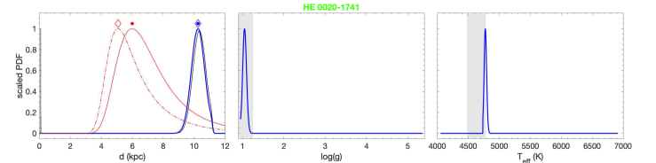
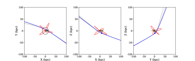
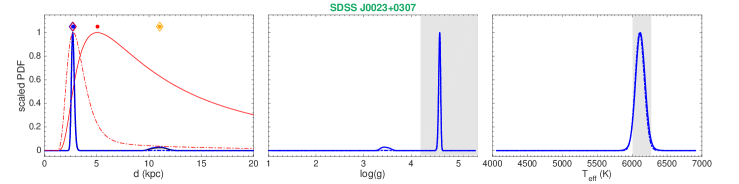
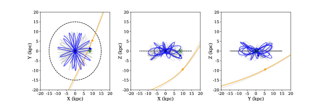
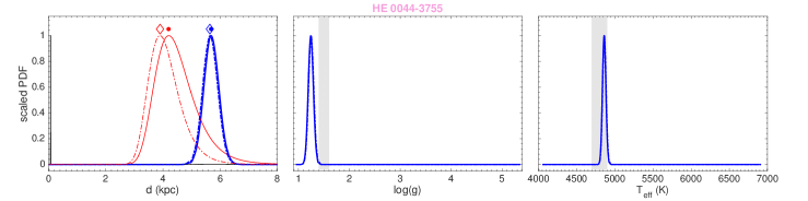
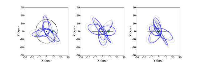
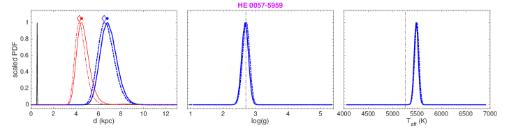
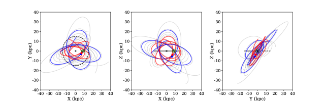
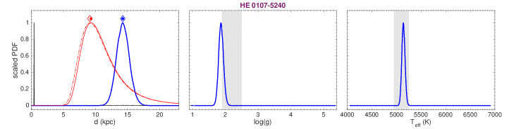
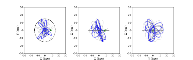
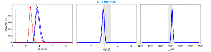
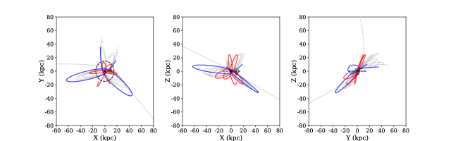
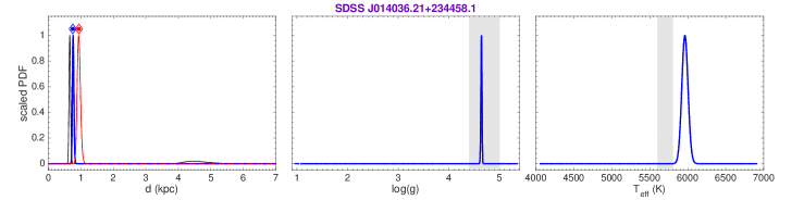

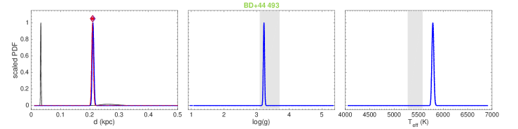
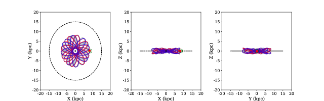
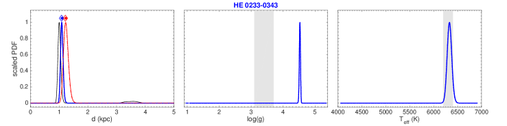
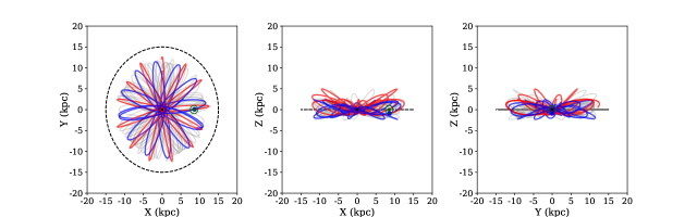
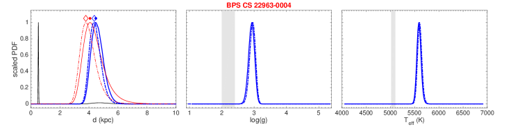
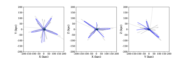
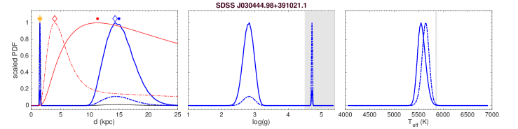
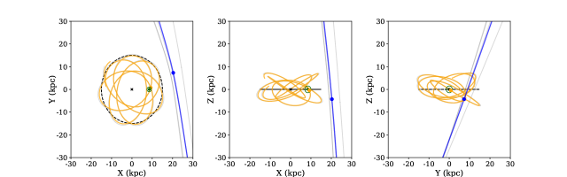
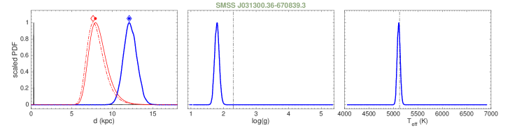
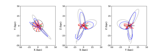
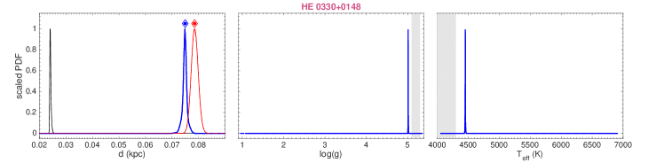
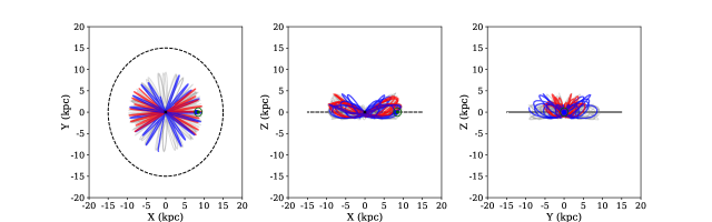
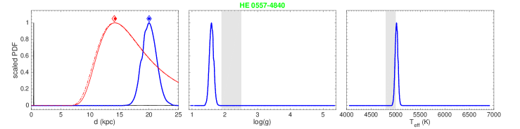
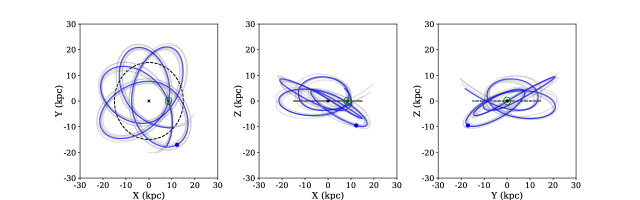
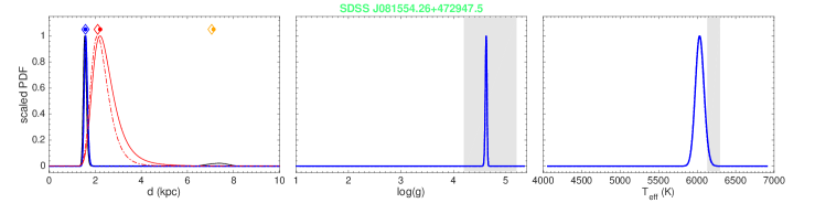
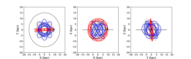
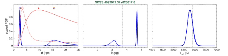
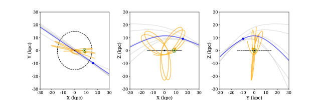
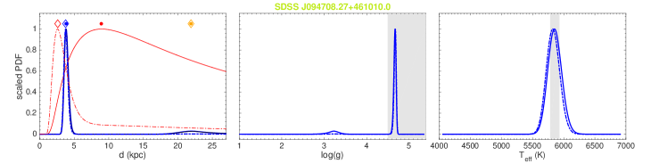
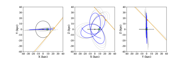
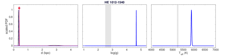
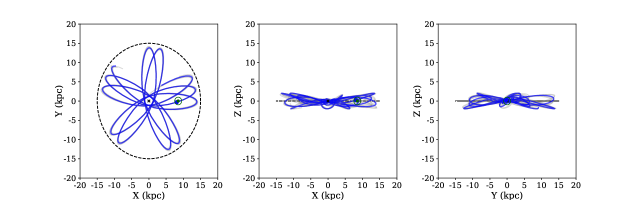

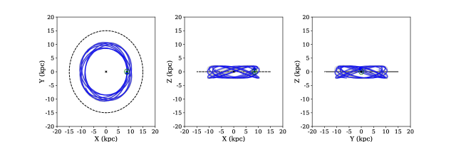
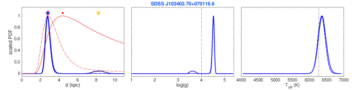
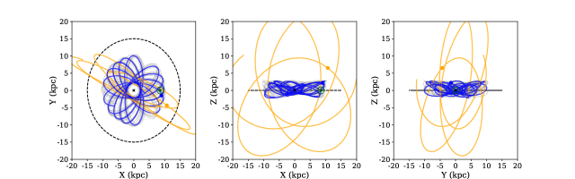
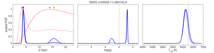
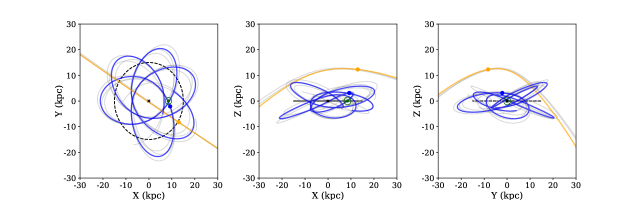
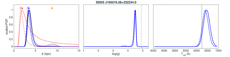
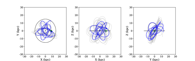
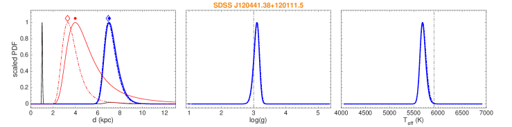
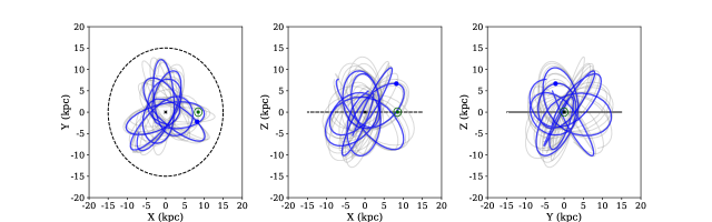
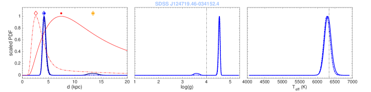
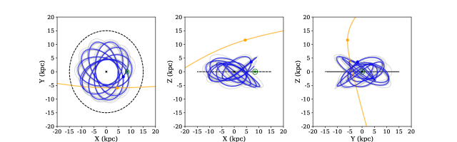
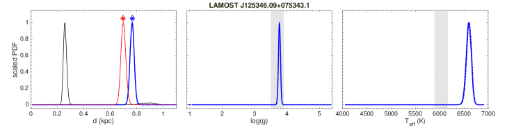
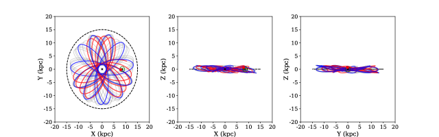
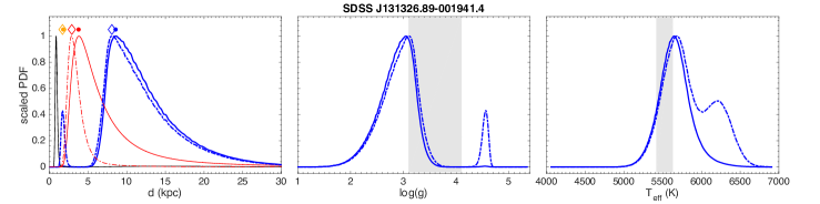
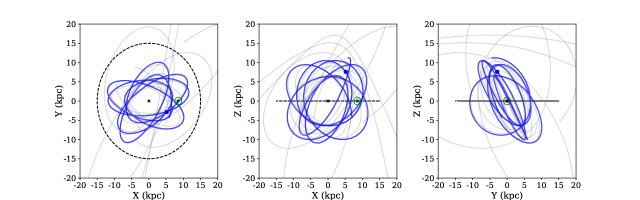
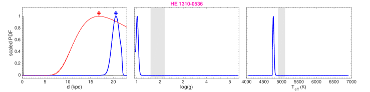
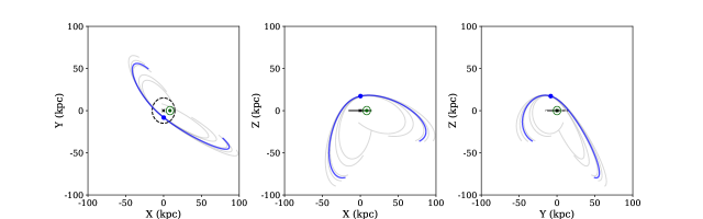
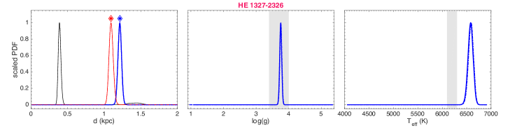
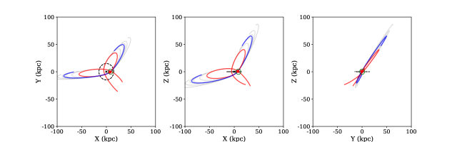
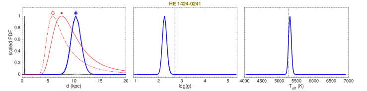
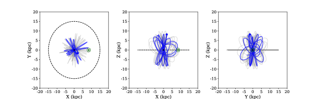
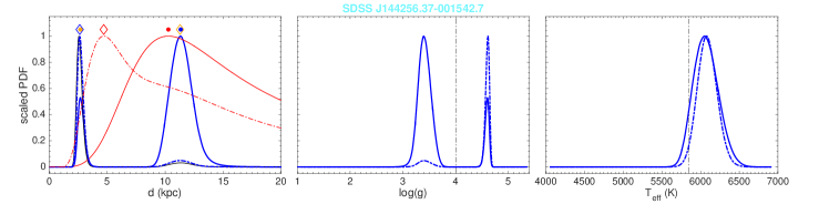
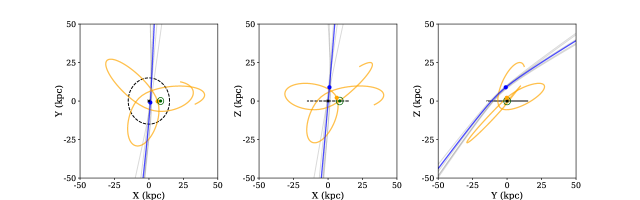
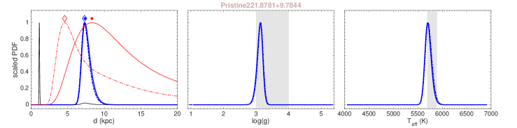
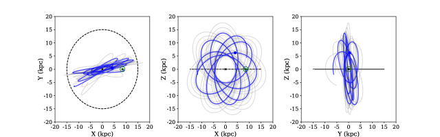
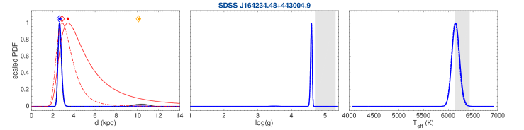
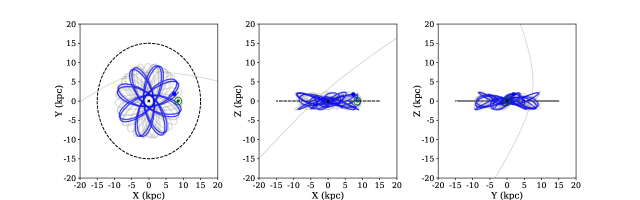
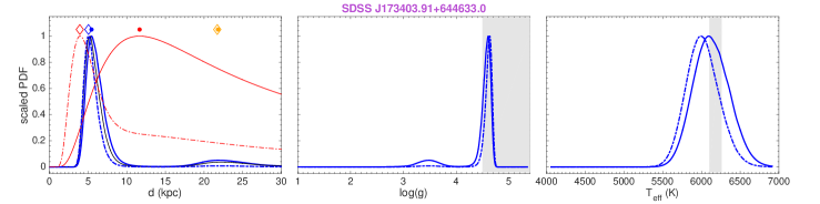
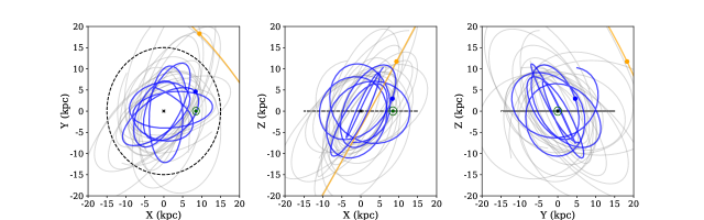
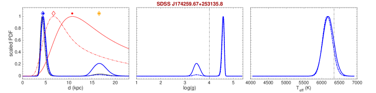
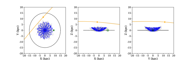
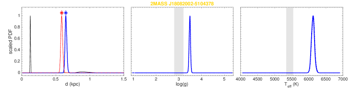
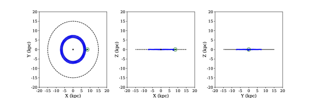
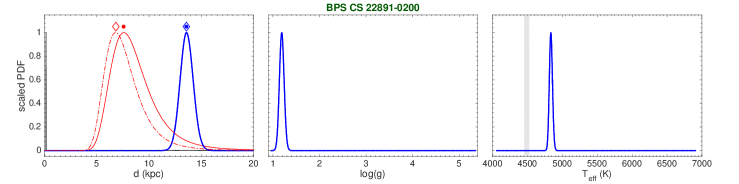
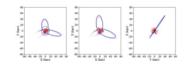
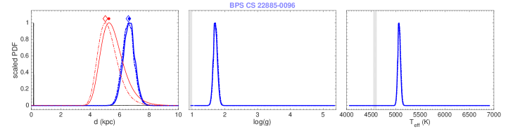
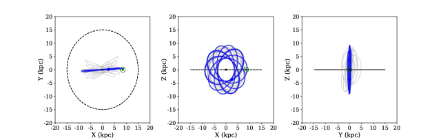
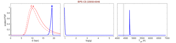
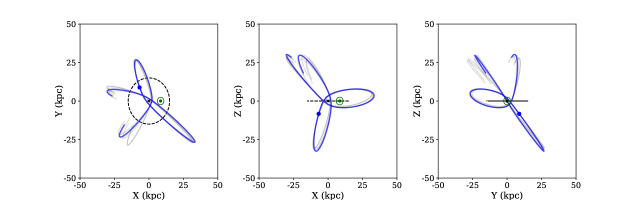
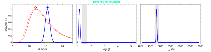
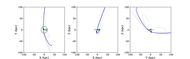
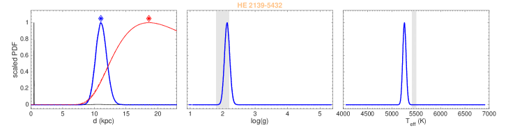
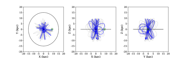
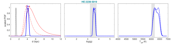
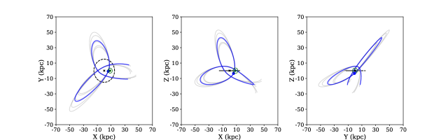
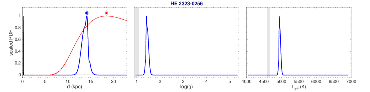
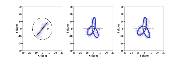
Appendix B Comparison with values from the literature
A global comparison between the stellar parameters inferred in this work and the values found in the literature is reported in the two panels of Figure 46. As we can see, we find a broad agreement for the effective temperature (left panel) and the surface gravity (right panel). Possible systematics are involved both in our method (e.g. relation in the MESA/MIST isochrones) and the multiple spectroscopic methods used by different authors (e.g. grid based models, synthetic spectra, data-driven analysis etc.).