Characterizing Well-Behaved vs. Pathological Deep Neural Networks
Abstract
We introduce a novel approach, requiring only mild assumptions, for the characterization of deep neural networks at initialization. Our approach applies both to fully-connected and convolutional networks and easily incorporates batch normalization and skip-connections. Our key insight is to consider the evolution with depth of statistical moments of signal and noise, thereby characterizing the presence or absence of pathologies in the hypothesis space encoded by the choice of hyperparameters. We establish: (i) for feedforward networks, with and without batch normalization, the multiplicativity of layer composition inevitably leads to ill-behaved moments and pathologies; (ii) for residual networks with batch normalization, on the other hand, skip-connections induce power-law rather than exponential behaviour, leading to well-behaved moments and no pathology.111Code to reproduce all results in this paper is available at https://github.com/alabatie/moments-dnns.
medium1\scalebox1.1\BODY \NewEnvironmedium2\scalebox1.05\BODY
1 Introduction
The feverish pace of practical applications has led in the recent years to many advances in neural network architectures, initialization and regularization. At the same time, theoretical research has not been able to follow the same pace. In particular, there is still no mature theory able to validate the full choices of hyperparameters leading to state-of-the-art performance. This is unfortunate since such theory could also serve as a guide towards further improvement.
Amidst the research aimed at building this theory, an important branch has focused on neural networks at initialization. Due to the randomness of model parameters at initialization, characterizing neural networks at that time can be seen as characterizing the hypothesis space of input-output mappings that will be favored or reachable during training, i.e. the inductive bias encoded by the choice of hyperparameters. This view has received strong experimental support, with well-behaved input-output mappings at initialization extensively found to be predictive of trainability and post-training performance (Schoenholz et al., 2017; Yang & Schoenholz, 2017; Xiao et al., 2018; Philipp & Carbonell, 2018; Yang et al., 2019).
Yet, even this simplifying case of neural networks at initialization is challenging as it notably involves dealing with: (i) the complex interplay of the randomness from input data and from model parameters; (ii) the broad spectrum of potential pathologies; (iii) the finite number of units in each layer; (iv) the difficulty to incorporate convolutional layers, batch normalization and skip-connections. Complexities (i), (ii) typically lead to restricting to specific cases of input data and pathologies, e.g. exploding complexity of data manifolds (Poole et al., 2016; Raghu et al., 2017), exponential correlation or decorrelation of two data points (Schoenholz et al., 2017; Balduzzi et al., 2017; Xiao et al., 2018), exploding and vanishing gradients (Yang & Schoenholz, 2017; Philipp et al., 2018; Hanin, 2018; Yang et al., 2019), exploding and vanishing activations (Hanin & Rolnick, 2018). Complexity (iii) commonly leads to making simplifying assumptions, e.g. convergence to Gaussian processes for infinite width (Neal, 1996; Le Roux & Bengio, 2007; Lee et al., 2018; Matthews et al., 2018; Borovykh, 2018; Garriga-Alonso et al., 2019; Novak et al., 2019; Yang, 2019), “typical” activation patterns (Balduzzi et al., 2017). Finally complexity (iv) most often leads to limiting the number of hard-to-model elements incorporated at a time. To the best of our knowledge, all attempts have thus far been limited in either their scope or their simplifying assumptions.
As the first contribution of this paper, we introduce a novel approach for the characterization of deep neural networks at initialization. This approach: (i) offers a unifying treatment of the broad spectrum of pathologies without any restriction on the input data; (ii) requires only mild assumptions; (iii) easily incorporates convolutional layers, batch normalization and skip-connections.
As the second contribution, we use this approach to characterize deep neural networks with the most common choices of hyperparameters. We identify the multiplicativity of layer composition as the driving force towards pathologies in feedforward networks: either with the neural network having its signal shrunk into a single point or line; or with the neural network behaving as a noise amplifier with sensitivity exploding with depth. In contrast, we identify the combined action of batch normalization and skip-connections as responsible for bypassing this multiplicativity and relieving from pathologies in batch-normalized residual networks.
2 Propagation
We start by formulating the propagation for neural networks with neither batch normalization nor skip-connections, that we refer as vanilla nets. We will slightly adapt this formulation in Section 6 with batch-normalized feedforward nets and in Section 7 with batch-normalized resnets.
Clean Propagation. We first consider a random tensorial input , spatially -dimensional with extent in all spatial dimensions and channels. This input is fed into a -dimensional convolutional neural network with periodic boundary conditions, fixed spatial extent , and activation function .222It is possible to relax the assumptions of periodic boundary conditions and constant spatial extent [B.5]. These assumptions, as well as the assumption of constant width in Section 7, are only made for simplicity of the analysis. At each layer , we denote the number of channels or width, the convolutional spatial extent, the post-activations and pre-activations, the weights, and the biases. Later in our analysis, the model parameters , will be considered as random, but for now they are considered as fixed. At each layer, the propagation is given by
with the convolution and the tensor with repeated version of at each spatial position. From now on, we refer to the propagated tensor as the signal.
Noisy Propagation. To make our setup more realistic, we next suppose that the input signal is corrupted by an input noise having small iid components such that , with and the Kronecker delta for multidimensional indices . We denote , with the neural network mapping from layer to , and we consider the simultaneous propagation of the signal and the noise . At each layer, this simultaneous propagation is given at first order by
| (1) | ||||||
| (2) |
with the element-wise tensor multiplication. The tensor resulting from the simultaneous propagation of in Eq. (1) and Eq. (2) approximates arbitrarily well the noise as [C.1]. For simplicity, we will keep the terminology of noise when referring to .
From Eq. (1) and Eq. (2), we see that , only depend on the input signal , and that depends linearly on the input noise when is fixed. As a consequence, stays centered with respect to such that : , where from now on the spatial position is denoted as and the channel as c.
Scope. We require two mild assumptions: (i) is not trivially zero: ;333Whenever and c are considered as random variables, they are supposed uniformly sampled among all spatial positions and all channels . (ii) the width is bounded.
Some results of our analysis will apply for any choice of , but unless otherwise stated, we restrict to the most common choice: . Even though is not differentiable at , we still define as the result of the simultaneous propagation of in Eq. (1) and Eq. (2) with the convention [C.2].
Note that fully-connected networks are included in our analysis as the subcase .
3 Data Randomness
Now we may turn our attention to the data distributions of signal and noise: , . To outline the importance of these distributions, the output of an -layer neural network can be expressed by layer composition as , with the mapping of the signal and noise by the upper neural network from layer to layer . The upper neural network thus receives as input signal and as input noise, implying that it can only have a chance to do any better than random guessing when: (i) is meaningful; (ii) is under control. Namely, when , are not affected by pathologies. We will make this argument as well as the notion of pathology more precise in Section 3.2 after a few prerequisite definitions.
3.1 Characterizing Data Distributions
Using as a placeholder for any tensor of layer in the simultaneous propagation of – e.g. , , , in Eq. (1) and Eq. (2) – we define:
– The feature map vector and centered feature map vector,
with the vectorial slice of at spatial position . Note that , aggregate both the randomness from which determines the propagation up to , and the randomness from which determines the spatial position in . These random vectors will enable us to circumvent the tensorial structure of .
– The non-central moment and central moment of order for given channel c and averaged over channels,
In the particular case of the noise , centered with respect to , feature map vectors and centered feature map vectors coincide: , such that non-central moments and central moments also coincide: and .
– The effective rank (Vershynin, 2010),
with the covariance matrix and the spectral norm. If we further denote the eigenvalues of , then . Intuitively, measures the number of effective directions which concentrate the variance of .
– The normalized sensitivity – our key metric – derived from the moments of and ,
| (3) |
To grasp the definition of , we may consider the signal-to-noise ratio and the noise factor ,
| (4) |
We obtain in logarithmic decibel scale, i.e. that measures how the neural network from layer to degrades () or enhances () the input signal-to-noise ratio. Neural networks with are noise amplifiers, while neural networks with are noise reducers.
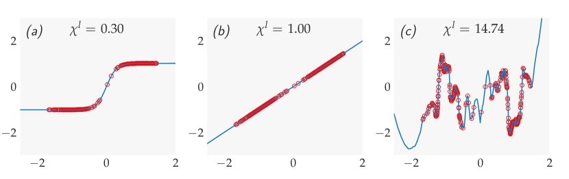
Now, to justify our choice of terminology, let us reason in the case where is the output signal at the final layer. Then: (i) the variance is typically constrained by the task (e.g. binary classification constrains to be roughly equal to ); (ii) the constant rescaling leads to the same constrained variance: . The normalized sensitivity exactly measures the excess root mean square sensitivity of the neural network mapping relative to the constant rescaling [C.3]. This property is illustrated in Fig. 1.
As outlined, measures the sensitivity to signal perturbation, which is known for being connected to generalization (Rifai et al., 2011; Arpit et al., 2017; Sokolic et al., 2017; Arora et al., 2018; Morcos et al., 2018; Novak et al., 2018; Philipp & Carbonell, 2018). A tightly connected notion is the sensitivity to weight perturbation, also known for being connected to generalization (Hochreiter & Schmidhuber, 1997; Langford & Caruana, 2002; Keskar et al., 2017; Chaudhari et al., 2017; Smith & Le, 2018; Dziugaite & Roy, 2017; Neyshabur et al., 2017, 2018; Li et al., 2018). The connection is seen by noting the equivalence between a noise on the weights and a noise and on the signal in Eq. (1) and Eq. (2).
3.2 Characterizing Pathologies
We are now able to characterize the pathologies, with ill-behaved data distributions, , , that we will encounter:
– Zero-dimensional signal: . To understand this pathology, let us consider the following mean vectors and rescaling of the signal:
The pathology implies , meaning that becomes point-like concentrated at the point of unit norm: [C.4]. In the limit of strict point-like concentration, the upper neural network from layer to is limited to random guessing since it “sees” all inputs the same and cannot distinguish between them.
– One-dimensional signal: . This pathology implies that the variance of becomes concentrated in a single direction, meaning that becomes line-like concentrated. In the limit of strict line-like concentration, the upper neural network from layer to only “sees” a single feature from .
– Exploding sensitivity: for some . Given the noise factor equivalence of Eq. (4), the pathology implies , meaning that the clean signal becomes drowned in the noise . In the limit of strictly zero signal-to-noise ratio, the upper neural network from layer to is limited to random guessing since it only “sees” noise.
4 Model Parameters Randomness
We now introduce model parameters as the second source of randomness. We consider networks at initialization, which we suppose is standard following He et al. (2015): (i) weights are initialized with , biases are initialized with zeros; (ii) when pre-activations are batch-normalized, scale and shift batch normalization parameters are initialized with ones and zeros respectively.
Considering networks at initialization is justified in two respects. As the first justification, in the context of Bayesian neural networks, the distribution on model parameters at initialization induces a distribution on input-output mappings which can be seen as the prior encoded by the choice of hyperparameters (Neal, 1996; Williams, 1997).
As the second justification, even in the standard context of non-Bayesian neural networks, it is likely that pathologies at initialization penalize training by hindering optimization. Let us illustrate this argument in two cases:
– In the case of zero-dimensional signal, the upper neural network from layer to must adjust its bias parameters very precisely in order to center the signal and distinguish between different inputs. This case – further associated with vanishing gradients for bounded (Schoenholz et al., 2017) – is known as the “ordered phase” with unit correlation between different inputs, resulting in untrainability (Schoenholz et al., 2017; Xiao et al., 2018).
– In the case of exploding sensitivity, the upper neural network from layer to only “sees” noise and its backpropagated gradient is purely noise. Gradient descent then performs random steps and training loss is not decreased. This case – further associated with exploding gradients for batch-normalized or bounded (Schoenholz et al., 2017) – is known as the “chaotic phase” with decorrelation between different inputs, also resulting in untrainability (Schoenholz et al., 2017; Yang & Schoenholz, 2017; Xiao et al., 2018; Philipp & Carbonell, 2018; Yang et al., 2019).
From now on, our methodology is to consider all moment-related quantities, e.g. , , , , , , as random variables which depend on model parameters. We denote the model parameters as and use as shorthand for . We further denote the geometric increments of as .
Evolution with Depth. The evolution with depth of can be written as
where we used and expressed with telescoping terms. Denoting the multiplicatively centered increments of , we get [C.5]
| (5) | ||||
| (6) | ||||
| (7) |
Discussion. We directly note that: (i) and are random variables which depend on , while is a random variable which depends on ; (ii) by log-concavity; (iii) is centered with and .
We further note that each channel provides an independent contribution to , implying for large that has low expected deviation to and that , , with high probability. The term is thus dominating as long as it is not vanishing. The same reasoning applies to other positive moments, e.g. , .
Further Notation. From now on, the geometric increment of any quantity is denoted with . The definitions of , and in Eq. (5), (6) and (7) are extended to other positive moments of signal and noise, as well as with
We introduce the notation when with , with high probability. And the notation when with , with high probability. From now on, we assume that the width is large, implying
We stress the layer-wise character of this approximation, whose validity only requires , independently of the depth . This contrasts with the aggregated character (up to layer ) of the mean field approximation of as a Gaussian process, whose validity requires not only but also – as we will see – that the depth remains sufficiently small with respect to .
5 Vanilla Nets
We are fully equipped to characterize deep neural networks at initialization. We start by analyzing vanilla nets which correspond to the propagation introduced in Section 2.
Theorem 1 (moments of vanilla nets).
[D.3] There exist small constants , random variables , and events , of probabilities equal to such that
| Under : | ||||
| Under : |
Discussion. The conditionality on , is necessary to exclude the collapse: , , with undefined , , occurring e.g. when all elements of are strictly negative (Lu et al., 2018). In practice, this conditionality is highly negligible since the probabilities of the complementary events , decay exponentially in the width [D.4].
Now let us look at the evolution of , under , . The initialization He et al. (2015) enforces and such that: (i) , are kept stable during propagation; (ii) , vanish and , are subject to a slow diffusion with small negative drift terms: , , and small diffusion terms: , [D.5].555Any deviation from He et al. (2015) leads, on the other hand, to pathologies orthogonal to the pathologies of Section 3.2, with either exploding or vanishing constant scalings of . The diffusion happens in log-space since layer composition amounts to a multiplicative random effect in real space. It is a finite-width effect since the terms , , , also vanish for infinite width.
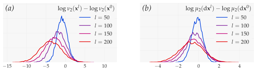
Fig. 2 illustrates the slowly decreasing negative expectation and slowly increasing variance of , , caused by the small negative drift and diffusion terms. Fig. 2 also indicates that , are nearly Gaussian, implying that , are nearly lognormal. Two important insights are then provided by the expressions of the expectation: and the kurtosis: of a lognormal variable with . Firstly, the decreasing negative expectation and increasing variance of , act as opposing forces in order to ensure the stabilization of , . Secondly, , are stabilized only in terms of expectation and they become fat-tailed distributed as .
Theorem 2 (normalized sensitivity increments of vanilla nets).
Discussion. A first consequence is that always increases with depth. Another consequence is that only two possibilities of evolution which both lead to pathologies are allowed:
– If sensitivity is exploding: with exponential drift stronger than the slow diffusion of Theorem 1 and if , are lognormally distributed as supported by Fig. 2, then Theorem 1 implies the a.s. convergence to the pathology of zero-dimensional signal: [D.7].
– Otherwise, geometric increments are strongly limited. In the limit , if the moments of remain bounded, then Theorem 2 implies the convergence to the pathology of one-dimensional signal: [D.8] and the convergence to pseudo-linearity, with each additional layer becoming arbitrarily well approximated by a linear mapping [D.9].
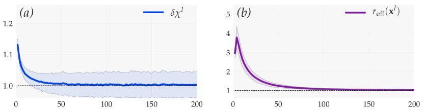
Experimental Verification. The evolution with depth of vanilla nets is shown in Fig. 3. From the two possibilities, we observe the case with limited geometric increments: , the convergence to the pathology of one-dimensional signal: , and the convergence to pseudo-linearity.
The only way that the neural network can achieve pseudo-linearity is by having each one of its units either always active or always inactive, i.e. behaving either as zero or as the identity. Our analysis offers theoretical insight into this coactivation phenomenon, previously observed experimentally (Balduzzi et al., 2017; Philipp et al., 2018).
6 Batch-Normalized Feedforward Nets
Next we incorporate batch normalization (Ioffe & Szegedy, 2015), which we denote as . For simplicity, we only consider the test mode which consists in subtracting and dividing by for each channel c in . The propagation is given by
| (9) | ||||||
| (10) | ||||||
| (11) |
Theorem 3 (normalized sensitivity increments of batch-normalized feedforward nets).
Effect of Batch Normalization. The batch normalization term is such that , with defined as the increment of in the convolution and batch normalization steps of Eq. (9) and Eq. (10). The expression of holds for any choice of .
This term can be understood intuitively by seeing the different channels c in as random projections of and batch normalization as a modulation of the magnitude for each projection. Since batch normalization uses as normalization factor, directions of high signal variance are dampened, while directions of low signal variance are amplified. This preferential exploration of low signal directions naturally deteriorates the signal-to-noise ratio and amplifies owing to the noise factor equivalence of Eq. (4).
Now let us look directly at in Theorem 3. If we define the event under which the vectorized weights in channel c have norm equal to : , then spherical symmetry implies that variance increments in channel c from to and from to have equal expectation under :
On the other hand, the variance of these increments depends on the fluctuation of signal and noise in the random direction generated by . This depends on the conditioning of signal and noise, i.e. on the magnitude of , . If we assume that is well-conditioned, then can be treated as a constant and by convexity of the function :
which in turn implies . The worse the conditioning of , i.e. the smaller , the larger the variance of at the denominator and the impact of the convexity. Thus the smaller and the larger . This argument is strictly valid for the first step of the propagation wherein the noise has perfect conditioning, resulting in [E.2].
Effect of the Nonlinearity. The nonlinearity term is such that , with defined as the increment of in the nonlinearity step of Eq. (11). This term is analogous to the term of Eq. (8) for vanilla nets, except that is less likely to vanish than in Eq. (8) since batch normalization now keeps the signal centered around zero.
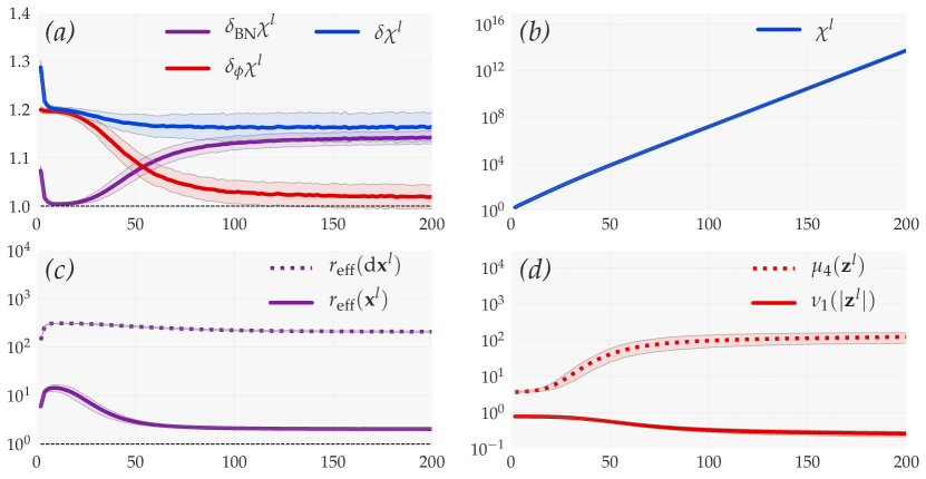
Experimental Verification. In Fig. 5, we confirm experimentally the pathology of exploding sensitivity: for some . We also confirm that: (i) remains well-conditioned, while becomes ill-conditioned; (ii) and are inversely correlated.
Interestingly, becomes subdominant with respect to at large depth. This stems from the fact that becomes fat-tailed distributed with respect to , , with large and small . Combined with and , this explains the decay of and thus of .
7 Batch-Normalized ResNets
We finish our exploration of deep neural network architectures with the incorporation of skip-connections. From now on, we assume that the width is constant, , and following He et al. (2016), we adopt the perspective of pre-activation units. The propagation is given by
| (12) |
If we adopt the convention , then Eq. (12) can be expanded as
| (13) |
For consistency reasons, we redefine the inputs of the propagation as and the normalized sensitivity and its increments as
| , | |||||||
| , |
Theorem 4 (normalized sensitivity increments of batch-normalized resnets).
[F.3] Suppose that we can bound signal variances: and feedforward increments: for all . Further denote and , as well as and . Then there exist positive constants , such that
| (14) | ||||||
| (15) |
Discussion. First let us note that Theorem 4 remarkably holds for any choice of , with and without batch normalization, as long as the existence of , , , is ensured. In the case , the existence of , is always ensured but the existence of , is only ensured when batch normalization controls signal variance inside residual units: [F.4].
Now let us get a better grasp of Theorem 4. We see in Eq. (14) that the evolution remains exponential inside residual units since , have an exponential dependence in . However, it is slowed down by the factor between successive residual units. This stems from the dilution (Philipp et al., 2018) of the residual path into the skip-connection path with ratio of signal variances , decaying as . If we remove the dilution effect by multiplying the skip-connection branch by (i.e. replacing the scaling in by a scaling in ) and if we set , then Eq. (14) recovers the feedforward evolution . The dilution is clearly visible in Eq. (13). Namely, each residual unit adds a term of increased but its relative contribution to the aggregation gets smaller and smaller with , so that the growth of gets slower and slower with .
Since and for , the bounds on in Eq. (15) are obtained by integrating the bounds on the logarithm of Eq. (14). A direct consequence of the dilution is thus the power-law evolution of instead of the exponential evolution for feedforward nets. Equivalently, when rewriting Eq. (15) as
the evolution of for resnets is equivalent to the evolution of for some for feedforward nets. In other words, the evolution with depth of resnets is the logarithmic version of the evolution with depth of feedforward nets.
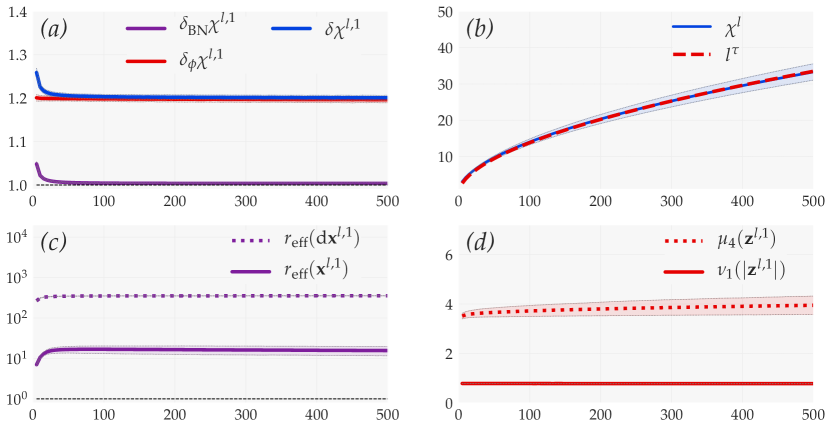
Experimental Verification. The evolution with depth of batch-normalized resnets is shown in Fig. 5. There is a clear parallel between the evolution for in Fig. 5 and the evolution for in Fig. 5. This confirms that batch-normalized resnets are slower-to-evolve variants of batch-normalized feedforward nets.
The exponent in the power-law fit of Fig. 4(f) is notably set to , with the feedforward increment averaged over the whole evolution. This means that Eq. (15) very well describes the evolution of in practice.
Contrary to batch-normalized feedforward nets, the signal remains well-behaved with: (i) many directions of signal variance preserved in ; (ii) close to Gaussian data distribution, as indicated e.g. by close to the Gaussian kurtosis of . No pathology occurs.
8 Discussion and Summary
The novel approach that we introduced for the characterization of deep neural networks at initialization brings three main contributions: (i) it offers a unifying treatment of the broad spectrum of pathologies; (ii) it relies on mild assumptions; (iii) it easily incorporates convolutional layers, batch normalization and skip connections.
Most studies on the convergence of neural networks to Gaussian processes have until now considered the maximal depth as constant and the width in the limit for . We reversed this perspective by considering the width as large but still bounded and the depth in the limit . Then the mean-field approximation of as a Gaussian process indexed by eventually becomes invalid:
– In the context of vanilla nets, with e.g. an input constant with respect to and reduced to a single point of such that remains a single point of . Given the evolution of Fig. 2, the norm becomes fat-tailed distributed as . For given , this means that and become fat-tailed distributed as .
– In the context of batch-normalized feedforward nets, with e.g. an input constant with respect to and uniformly sampled among points positioned spherically symmetrically in . Given the evolution of Fig. 5, spherical symmetry, together with batch normalization, implies that for any given : , , and . For given , this means that and become fat-tailed distributed as .
Similar observations were made in previous works. Duvenaud et al. (2014) found that the composition of Gaussian processes eventually leads to lognormal and ill-behaved derivatives; Matthews et al. (2018) found that the convergence to Gaussianity as becomes slower with respect to as the depth grows. This stems from the fact that the affine transform at each layer is additive with respect to the width dimension, but layer composition is multiplicative with respect to the depth dimension. Intuitively, the Central Limit Theorem implies that becomes normally distributed as , but lognormally distributed (with fat-tail) as .
Beside from this insight, our approach enabled us to characterize deep neural networks with the most common choices of hyperparameters:
– In the case of vanilla nets, the initialization He et al. (2015) limits the evolution of second-order moments of signal and noise. Combined with the limited growth of , this results in the convergence to the pathology of one-dimensional signal: and the convergence to neural network pseudo-linearity, with each additional layer becoming arbitrarily well approximated by a linear mapping.
– In the case of batch-normalized feedforward nets, the pathology of exploding sensitivity: for some has two origins: on the one hand, batch normalization which upweights low-signal pre-activation directions; on the other hand, the nonlinearity .
– Finally in the case of resnets, only grows as a power-law. Equivalently, the evolution with depth of resnets is the logarithmic version of the evolution with depth of feedforward nets. The underlying phenomenon is the dilution of the residual path into the skip-connection path with ratio of signal variances decaying as . This mechanism is responsible for breaking the circle of depth multiplicativity which causes pathologies for feedforward nets.
Acknowledgements
Many thanks are due to Jean-Baptiste Fiot for his precious feedback on initial drafts and to the anonymous reviewers for their insightful comments.
References
- Arora et al. (2018) Arora, S., Ge, R., Neyshabur, B., and Zhang, Y. Stronger generalization bounds for deep nets via a compression approach. In 35th International Conference on Machine Learning, pp. 254–263, 2018. URL http://proceedings.mlr.press/v80/arora18b.html.
- Arpit et al. (2017) Arpit, D., Jastrzebski, S. K., Ballas, N., Krueger, D., Bengio, E., Kanwal, M. S., Maharaj, T., Fischer, A., Courville, A. C., Bengio, Y., and Lacoste-Julien, S. A closer look at memorization in deep networks. In 34th International Conference on Machine Learning, pp. 233–242, 2017. URL http://proceedings.mlr.press/v70/arpit17a.html.
- Balduzzi et al. (2017) Balduzzi, D., Frean, M., Leary, L., Lewis, J. P., Ma, K. W., and McWilliams, B. The shattered gradients problem: If resnets are the answer, then what is the question? In 34th International Conference on Machine Learning, pp. 342–350, 2017. URL http://proceedings.mlr.press/v70/balduzzi17b.html.
- Billingsley (1995) Billingsley, P. Probability and Measure. Wiley, 1995.
- Borovykh (2018) Borovykh, A. A gaussian process perspective on convolutional neural networks. arXiv preprint, 2018. URL https://arxiv.org/abs/1810.10798.
- Chaudhari et al. (2017) Chaudhari, P., Choromanska, A., Soatto, S., LeCun, Y., Baldassi, C., Borgs, C., Chayes, J., Sagun, L., and Zecchina, R. Entropy-sgd: Biasing gradient descent into wide valleys. In International Conference on Learning Representations, 2017. URL https://openreview.net/forum?id=B1YfAfcgl.
- Chiani et al. (2003) Chiani, M., Dardari, D., and Simon, M. K. New exponential bounds and approximations for the computation of error probability in fading channels. IEEE Transactions on Wireless Communications, 2(4):840–845, 2003. URL https://core.ac.uk/download/pdf/11174040.pdf.
- Duvenaud et al. (2014) Duvenaud, D., Rippel, O., Adams, R., and Ghahramani, Z. Avoiding pathologies in very deep networks. In 17th International Conference on Artificial Intelligence and Statistics, pp. 202–210, 2014. URL http://proceedings.mlr.press/v33/duvenaud14.html.
- Dziugaite & Roy (2017) Dziugaite, G. K. and Roy, D. M. Computing nonvacuous generalization bounds for deep (stochastic) neural networks with many more parameters than training data. In 33rd Conference on Uncertainty in Artificial Intelligence, 2017. URL http://auai.org/uai2017/proceedings/papers/173.pdf.
- Garriga-Alonso et al. (2019) Garriga-Alonso, A., Rasmussen, C. E., and Aitchison, L. Deep convolutional networks as shallow gaussian processes. In International Conference on Learning Representations, 2019. URL https://openreview.net/forum?id=Bklfsi0cKm.
- Hanin (2018) Hanin, B. Which neural net architectures give rise to exploding and vanishing gradients? In Advances in Neural Information Processing Systems 31, pp. 580–589, 2018. URL http://papers.nips.cc/paper/7339-which-neural-net-architectures-give-rise-to-exploding-and-vanishing-gradients.
- Hanin & Rolnick (2018) Hanin, B. and Rolnick, D. How to start training: The effect of initialization and architecture. In Advances in Neural Information Processing Systems 31, pp. 569–579, 2018. URL http://papers.nips.cc/paper/7338-how-to-start-training-the-effect-of-initialization-and-architecture.
- He et al. (2015) He, K., Zhang, X., Ren, S., and Sun, J. Delving deep into rectifiers: Surpassing human-level performance on imagenet classification. In International Conference on Computer Vision, pp. 1026–1034, 2015. URL http://dx.doi.org/10.1109/ICCV.2015.123.
- He et al. (2016) He, K., Zhang, X., Ren, S., and Sun, J. Identity mappings in deep residual networks. In 14th European Conference on Computer Vision, pp. 630–645, 2016. URL https://doi.org/10.1007/978-3-319-46493-0_38.
- Hochreiter & Schmidhuber (1997) Hochreiter, S. and Schmidhuber, J. Flat minima. Neural Computation, 9(1):1–42, 1997. URL http://dx.doi.org/10.1162/neco.1997.9.1.1.
- Ioffe & Szegedy (2015) Ioffe, S. and Szegedy, C. Batch normalization: Accelerating deep network training by reducing internal covariate shift. In 32nd International Conference on Machine Learning, pp. 448–456, 2015. URL http://jmlr.org/proceedings/papers/v37/ioffe15.html.
- Keskar et al. (2017) Keskar, N. S., Mudigere, D., Nocedal, J., Smelyanskiy, M., and Tang, P. T. P. On large-batch training for deep learning: Generalization gap and sharp minima. In International Conference on Learning Representations, 2017. URL https://openreview.net/forum?id=H1oyRlYgg.
- Langford & Caruana (2002) Langford, J. and Caruana, R. (not) bounding the true error. In Advances in Neural Information Processing Systems 14, pp. 809–816, 2002. URL http://papers.nips.cc/paper/1968-not-bounding-the-true-error.
- Le Roux & Bengio (2007) Le Roux, N. and Bengio, Y. Continuous neural networks. In 11th International Conference on Artificial Intelligence and Statistics, pp. 404–411, 2007. URL http://proceedings.mlr.press/v2/leroux07a.html.
- Lee et al. (2018) Lee, J., Sohl-dickstein, J., Pennington, J., Novak, R., Schoenholz, S., and Bahri, Y. Deep neural networks as gaussian processes. In International Conference on Learning Representations, 2018. URL https://openreview.net/forum?id=B1EA-M-0Z.
- Li et al. (2018) Li, H., Xu, Z., Taylor, G., Studer, C., and Goldstein, T. Visualizing the loss landscape of neural nets. In Advances in Neural Information Processing Systems 31, pp. 6391–6401, 2018. URL http://papers.nips.cc/paper/7875-visualizing-the-loss-landscape-of-neural-nets.
- Lu et al. (2018) Lu, L., Su, Y., and Karniadakis, G. E. Collapse of deep and narrow neural nets. arXiv preprint, 2018. URL http://arxiv.org/abs/1808.04947.
- Matthews et al. (2018) Matthews, A. G., Rowland, M., Hron, J., Turner, R. E., and Ghahramani, Z. Gaussian process behaviour in wide deep neural networks. arXiv preprint, 2018. URL https://arxiv.org/abs/1804.11271.
- Morcos et al. (2018) Morcos, A. S., Barrett, D. G., Rabinowitz, N. C., and Botvinick, M. On the importance of single directions for generalization. In International Conference on Learning Representations, 2018. URL https://openreview.net/forum?id=r1iuQjxCZ.
- Neal (1996) Neal, R. M. Bayesian Learning for Neural Networks. Springer-Verlag, 1996.
- Neyshabur et al. (2017) Neyshabur, B., Bhojanapalli, S., Mcallester, D., and Srebro, N. Exploring generalization in deep learning. In Advances in Neural Information Processing Systems 30, pp. 5947–5956, 2017. URL http://papers.nips.cc/paper/7176-exploring-generalization-in-deep-learning.
- Neyshabur et al. (2018) Neyshabur, B., Bhojanapalli, S., and Srebro, N. A PAC-bayesian approach to spectrally-normalized margin bounds for neural networks. In International Conference on Learning Representations, 2018. URL https://openreview.net/forum?id=Skz_WfbCZ.
- Novak et al. (2018) Novak, R., Bahri, Y., Abolafia, D. A., Pennington, J., and Sohl-Dickstein, J. Sensitivity and generalization in neural networks: an empirical study. In International Conference on Learning Representations, 2018. URL https://openreview.net/forum?id=HJC2SzZCW.
- Novak et al. (2019) Novak, R., Xiao, L., Bahri, Y., Lee, J., Yang, G., Abolafia, D. A., Pennington, J., and Sohl-dickstein, J. Deep bayesian convolutional networks with many channels are gaussian processes. In International Conference on Learning Representations, 2019. URL https://openreview.net/forum?id=B1g30j0qF7.
- Philipp & Carbonell (2018) Philipp, G. and Carbonell, J. G. The nonlinearity coefficient - predicting overfitting in deep neural networks. arXiv preprint, 2018. URL http://arxiv.org/abs/1806.00179.
- Philipp et al. (2018) Philipp, G., Song, D., and Carbonell, J. G. Gradients explode - deep networks are shallow - resnet explained. In International Conference on Learning Representations - Workshop Track, 2018. URL https://openreview.net/forum?id=HkpYwMZRb.
- Poole et al. (2016) Poole, B., Lahiri, S., Raghu, M., Sohl-Dickstein, J., and Ganguli, S. Exponential expressivity in deep neural networks through transient chaos. In Advances in Neural Information Processing Systems 29, pp. 3360–3368, 2016. URL http://papers.nips.cc/paper/6322-exponential-expressivity-in-deep-neural-networks-through-transient-chaos.
- Raghu et al. (2017) Raghu, M., Poole, B., Kleinberg, J., Ganguli, S., and Sohl-Dickstein, J. On the expressive power of deep neural networks. In 34th International Conference on Machine Learning, pp. 2847–2854, 2017. URL http://proceedings.mlr.press/v70/raghu17a.html.
- Rifai et al. (2011) Rifai, S., Vincent, P., Muller, X., Glorot, X., and Bengio, Y. Contractive auto-encoders: Explicit invariance during feature extraction. In 28th International Conference on Machine Learning, pp. 833–840, 2011. URL http://www.iro.umontreal.ca/~lisa/pointeurs/ICML2011_explicit_invariance.pdf.
- Schoenholz et al. (2017) Schoenholz, S. S., Gilmer, J., Ganguli, S., and Sohl-Dickstein, J. Deep information propagation. In International Conference on Learning Representations, 2017. URL https://openreview.net/forum?id=H1W1UN9gg.
- Smith & Le (2018) Smith, S. L. and Le, Q. V. A bayesian perspective on generalization and stochastic gradient descent. In International Conference on Learning Representations, 2018. URL https://openreview.net/forum?id=BJij4yg0Z.
- Sokolic et al. (2017) Sokolic, J., Giryes, R., Sapiro, G., and Rodrigues, M. R. D. Robust large margin deep neural networks. IEEE Transactions on Signal Processing, 65(16):4265–4280, 2017. URL https://doi.org/10.1109/TSP.2017.2708039.
- Vershynin (2010) Vershynin, R. Introduction to the non-asymptotic analysis of random matrices. arXiv preprint, 2010. URL http://arxiv.org/abs/1011.3027.
- Williams (1997) Williams, C. K. I. Computing with infinite networks. In Advances in Neural Information Processing Systems 9, pp. 295–301, 1997. URL http://papers.nips.cc/paper/1197-computing-with-infinite-networks.
- Xiao et al. (2018) Xiao, L., Bahri, Y., Sohl-Dickstein, J., Schoenholz, S., and Pennington, J. Dynamical isometry and a mean field theory of CNNs: How to train 10,000-layer vanilla convolutional neural networks. In 35th International Conference on Machine Learning, pp. 5393–5402, 2018. URL http://proceedings.mlr.press/v80/xiao18a.html.
- Yang (2019) Yang, G. Scaling limits of wide neural networks with weight sharing: Gaussian process behavior, gradient independence, and neural tangent kernel derivation. arXiv preprint, 2019. URL http://arxiv.org/abs/1902.04760.
- Yang & Schoenholz (2017) Yang, G. and Schoenholz, S. Mean field residual networks: On the edge of chaos. In Advances in Neural Information Processing Systems 30, pp. 7103–7114, 2017. URL http://papers.nips.cc/paper/6879-mean-field-residual-networks-on-the-edge-of-chaos.
- Yang et al. (2019) Yang, G., Pennington, J., Rao, V., Sohl-Dickstein, J., and Schoenholz, S. S. A mean field theory of batch normalization. In International Conference on Learning Representations, 2019. URL https://openreview.net/forum?id=SyMDXnCcF7.
Appendix A Details of the Experiments
Fig. 1 considered an input as a Gaussian mixture, with with probability and with probability . This input was propagated into: (a) a single layer with ; (b) a single layer with linear; (c) a batch-normalized feedforward net with: and for ; linear and for .
The experiments of Fig. 2, 3, 5, 5 were made on cifar10 with a random initial convolution of stride reducing the spatial dimension from to and increasing the width from to . In each case, we considered the convolutional extent and periodic boundary conditions.
In Fig. 2, we considered the width and the total depth . For each realization, we randomly initialized model parameters following He et al. (2015) and randomly sampled images to constitute the input data distribution. For each realization, we then computed the evolution with depth of and . The distributions of and shown in Fig. 2 were estimated using such realizations. The limited width – slightly smaller than standard values – had the purpose of limiting computation time in order to gather more realizations.
In Fig. 3, 5, 5, we increased the width to . For each realization, we randomly initialized model parameters following He et al. (2015) and randomly sampled images to constitute the input data distribution. We then computed the evolution with depth of all moment-related quantites. For each quantity, the expectation as well as the intervals displayed in Fig. 3, 5, 5 were estimated using such realizations.
Let us make a few remarks:
– The limited number of images for each experiment enabled to reduce the computation time, in particular penalized by the computation of , , , in Fig. 3, 5, 5. For batch-normalized feedforward nets and batch-normalized resnets, choosing in the range of standard batch sizes also had the advantage that our setup of batch normalization in test mode matched the usual setup of batch normalization in training mode.
For vanilla nets in Fig. 2, 3 and batch-normalized resnets in Fig. 5, this reduction of had very little impact. For batch-normalized feedforward nets in Fig. 5, on the other hand, this reduction of had the effect of limiting pathologies in the signal. This can be understood by considering batch-normalized random points . In our case, is proportional to but since the data distribution depends on the input and the spatial position . By considering the worst-case scenario such that :
This shows that the empirical kurtosis of is roughly bounded by , i.e. that the pathologies of the signal are naturally limited by the number of input images . As a result, for larger we found that: (i) gets closer to ; (ii) gets even larger and gets even smaller; (iii) and get larger; (iv) and get even smaller.
– The dynamics of at very low depth in Fig. 5, 5 stems from the input images from cifar10 having a number of channels equal to . The signal is therefore ill-conditioned at very low depth and quickly gets better conditioned, implying that is non-negligible at very low depth and quickly gets vanishing. This dynamics is brief and occurs before the settling of the main dynamics which leads in particular to the conditioning of the signal degrading again in Fig. 5.
– We tested to set more realistic values for the width in the experiment of Fig. 2. We always observed an absolutely equivalent behaviour apart from the diffusion getting slower with larger .
– We tested to change the boundary conditions from periodic to reflective and to zero-padding. We always observed an equivalent behaviour with reflective conditions. As for zero-padding conditions: (i) the evolution of vanilla nets was slightly changed with converging to a value of roughly instead of due to the creation of new signal directions by zero-padding; (ii) the evolution of batch-normalized feedforward nets and batch-normalized resnets were always equivalent.
– We tested to change the dataset from cifar10 to mnist, with the random initial convolution of stride reducing the spatial dimension from to and increasing the width from to . We observed an equivalent behaviour apart from the signal being slightly more fat-tailed at low depth due to the original images being more fat-tailed in mnist than in cifar10.
Appendix B Complementary Definitions and Notations
In this section, we use again as placeholder for any tensor of layer in the simultaneous propagation of .
B.1 Receptive Field
Receptive Field Mapping. Let us consider the convolution at layer of an input from layer . The output feature map of the convolution at position is obtained by the application of the convolution kernel over a local input region from of size , with the spatial extent and the channel extent. The local input region is called the receptive field of at spatial position .
The receptive field mapping associates to the tensor , with the reshaped vectorial form of the receptive field of at spatial position . We denote the dimensionality of and the set of indices in corresponding to elements in channel c in . Strictly speaking, depends on but this is implied by the argument, so we write for simplicity.
Receptive Field Vectors. The receptive field vector and centered receptive field vector associated with are defined as
where, slightly abusively, we overloaded the notation in the expectation. Again, strictly speaking, and depend on but this is implied by the argument.
B.2 Propagation with Receptive Field Formulation
Equation of Propagation. Using the definition of , the affine transformation from the receptive field to the feature map in the next layer can be written as
| (16) |
with the suitably reshaped matricial form of . To lighten notation, we write as a short for the affine transformation of Eq. (16) occuring at all spatial positions . We have the following equivalence between the notations with receptive field and convolution:
For vanilla nets, the simultaneous propagation of can be written as
For batch-normalized feedforward nets, the simultaneous propagation of can be written as
B.3 Symmetric Propagation
Symmetric Propagation for Vanilla Nets. We define additional tensors obtained by symmetric propagation at each layer . For vanilla nets, they are given by
Under standard initialization, the tensor moments have the same distribution with respect to for both propagations. Furthermore, : and , implying that : . Thus :
| (17) |
Now let us consider the second-order moments of the noise tensor:
| (18) |
where Eq. (18) was obtained using and , as well as the convention . Since , , are centered, it follows that :
| (19) |
Symmetric Propagation for Batch-Normalized Feedforward Nets. For batch-normalized feedforward nets, the symmetric propagation at each layer is given by
| (20) | ||||||
| (21) | ||||||
| (22) |
in Eq. (21) uses the statistics of such that, under standard initialization, the tensor moments have the same distribution with respect to for both propagations. We then simply have
| (23) |
The same analysis as before gives :
| (25) | ||||
| (26) |
B.4 Gramian and Covariance Matrices
We adopt the standard definition of the Gramian matrices of , , , :
Then, the covariance matrices of , , , are defined as
B.5 Statistics-Preserving Property
Statistics-Preserving Property. is statistics-preserving with respect to if for any channel c and any index , the random variables and , which depend on , , , have the same distribution: .
First we will prove that is statistics-preserving with respect to , when convolutions have periodic boundary conditions and the global spatial extent is constant. Afterwards, we will provide a possible relaxation of these assumptions. The global spatial extent will be denoted as when it is non-constant.
B.5.1 Case of Periodic Boundary Conditions and Constant Spatial Extent
Lemma 1.
If convolutions have periodic boundary conditions and the global spatial extent is constant, then is statistics-preserving with respect to any input from layer .
Proof.
Fix a channel c in , an index , and consider the tensors , . The index corresponds to a given convolution kernel position . Under periodic boundary conditions, this fixed kernel position implies that each position in originates from a different position in the tensor . Therefore the index mapping from to is bijective. We then have when is deterministic and is random. In turn, this implies that , when are random. ∎
Proposition 2.
If convolutions have periodic boundary conditions and the global spatial extent is constant, then is statistics-preserving with respect to and .
Proof. This follows immediately from Lemma 1. ∎
Corollary 3.
For any channel c and , we have and . Since the cardinality is the same for all channels c, it follows that
Note that this result always holds in the fully-connected case , characterized by , and .
B.5.2 Case of Large Spatial Extent
Proposition 4.
If the convolution stride is one (i.e. ) in most layers and the global spatial extent is much larger than the convolutional spatial extent (i.e. ) in most layers, then, for any boundary conditions, is approximately statistics-preserving with respect to and .
Proof. Fix a layer such that and . Denote the receptive field mapping associated with periodic boundary conditions. Since the receptive fields and do not intersect boundary regions for most , implying for most :
This implies for any index that and .
Since is statistics-preserving with respect to and by Lemma 1, it follows for any channel c and index that and . We then deduce that and , meaning that is approximately statistics-preserving with respect to and . ∎
Appendix C Details of Section 3 and Section 4
C.1 Approximation of by
We use the definitions and notations from Section B in the context of the propagation of Eq. (1) and Eq. (2). We further suppose that a.s. with respect to : such that is differentiable in the open ball of radius at point (see Section C.2 for the justification).
We will prove that
| (27) |
Due to the -Lipschitzness of , under periodic boundary conditions, we have that :
with the spectral norm of . It follows that :
This gives:
with .
The assumption on the differentiability of implies that , : . Markov’s inequality applied to further implies that
It then follows that , such that :
with .
Denoting the complementary event of , we deduce that :
| (28) | ||||
where we used Cauchy-Schwarz inequality in Eq. (28).
Since under , it follows that :
| (29) | ||||
Let us finally consider and such that . Then such that :
which proves Eq. (27).
C.2 Assumption that is Differentiable a.s. with respect to
The sensitivity equivalence detailed in Section C.3 relies on the assumption that is differentiable surely with respect to . If is differentiable a.s. with respect to , this can be relaxed using subdifferentials by noting that moments with respect to are left unchanged when ignoring zero-probability events.
Now let us justify the assumption that is differentiable a.s. with respect to in the context of the propagation of Eq. (1) and Eq. (2). We denote the receptive field vectors as in Section B, and we denote as in Section 4. We further assume standard initialization.
Let be an event depending on , , and let be the complementary event. We will prove that with probability with respect to .
For given such that : , it is easy to see that
Under standard initialization, this corresponds to a zero-probability event with respect to , meaning that .
Now considering again as random, using Fubini’s Theorem and making the assumption that a.s. with respect to (which is the case e.g. if has well-defined probability density function):
| (30) |
By contradiction, if there would be non-zero probability with respect to that , then Eq. (30) would not hold. Therefore with probability with respect to , , implying that with probability with respect to , is differentiable a.s. with respect to .
C.3 Property of Normalized Sensitivity
Proposition 5.
The noise tensor and the vectorized version of the tensor , containing for given the derivatives of with respect to , are related by: .
Proof. Due to the definition of as the first-order approximation of :
with the standard dot product in .
Then due to the white noise property: , we deduce that
| ∎ |
Proposition 6.
Denoting the neural network mapping and the constant rescaling leading to the same signal variance: , the normalized sensitivity exactly measures the excess root mean square sensitivty of the neural network mapping relative to the constant rescaling :
Proof. This directly follows from: (i) the definition of ; (ii) the result from Proposition 5; (iii) the fact that the constant rescaling has root mean square sensitivitiy equal to . ∎
C.4 Characterizing Pathologies
We consider the following mean vectors and rescaling of the signal:
We immediately have . Furthermore we have
The pathology implies , which in turn implies , i.e. . It follows that becomes point-like concentrated at point of unit norm.
C.5 Derivation of Eq. (5), (6) and (7)
The quantities , and are defined as
Denoting the multiplicatively centered increments of , the term can be expressed as
| (31) | ||||
where we used in Eq. (31). The term can be expressed as
| (32) | ||||
where we used again in Eq. (32).
Appendix D Details of Section 5
D.1 Lemmas on Weak Convergence
Weak Convergence. The sequence of random variables converges weakly to the random variable if for every continuity point of the function . We then write .
Tightness.
The sequence of random variables is tight if
Uniform Integrability.
The sequence of random variables is uniformly integrable if
Lemma 7 (Theorem 25.7 in Billingsley (1995)).
Consider a real-valued function , continuous everywhere apart from a finite set of discontinuity points . Then is measurable and if with , then .
Lemma 8 (Theorem 25.10 in Billingsley (1995), known as Prokhorov’s theorem).
If the sequence of random variables is tight, then it admits a weakly convergent subsequence, i.e. there exists a sequence of strictly increasing indices and a random variable such that .
Lemma 9 (Theorem 25.12 in Billingsley (1995)).
If the sequence of random variables is uniformly integrable and if , then has well-defined expectation and .
D.2 Lemma on the Sum of Increments
Lemma 10.
Let us consider a sequence of random variables and a decreasing sequence of events , which both depend on . Let us suppose that does not depend on and let us denote under :
Let us further suppose that there exist constants , , , such that , under :
Then it follows that
-
(i)
The random variables are centered and non-correlated such that , :
-
(ii)
There exist random variables and such that under :
Proof of (i).
First we show that is centered under :
| (33) | ||||
Now for , we have and thus is fully determined by . Then we can write
where we used Eq. (33). ∎
Proof
of (ii). First we note that
Combined with the hypothesis that , we deduce that
| (34) |
Now let us denote and . Then, using (i), we get that
| (35) |
D.3 Proof of Theorem 1
Theorem 1 (moments of vanilla nets). There exist small constants , random variables , and events , of probabilities equal to such that
| Under : | |||||||
| Under : |
D.3.1 Proof Introduction
Using the definitions and notations from Section B, denoting and respectively the orthogonal eigenvectors and eigenvalues of and denoting , we get that :
where we defined and used by Corollary 3.
Let us further define
Combined with by Eq. (17), we get that , under :
| (36) | ||||
| (37) |
Now combining Eq. (36) with the symmetry of the propagation: , and the assumption of standard initialization: , we get that , under :
Thus and , i.e. that under :
| (38) |
Next, let us define
with independent of and .
Conditionally on : , independently of and . And conditionally on : , independently of and . It follows that , independently of and .
Defining we get that . We also get that is independent of and thus of . This will be useful later in the course of this proof.
Denoting , we have that
where we used due to .
Now since and are independent, Eq. (37) implies that such that under :
On the other hand, such that under :
Denoting and the chi-squared distributions with and degrees of freedom respectively, such that under :
| (39) |
where we used .
Simply replacing by , by , by , using Eq. (19) instead of Eq. (17) and the identity with instead of in Corollary 3, we get that under :
| (40) |
Furthermore , independent of , such that , and such that under :
| (41) |
Denoting , we also have
Both and are integrable at since and . By Eq. (39) and Eq. (41), it then follows that and have well-defined expectation and variance under and respectively.
Now, crucially, let us note that the distributions of with respect to and with respect to are fully determined by: (i) the input distributions and ; (ii) the model parameters up to layer .
We are thus interested in the following infima and suprima:
| (42) | |||||
| (43) | |||||
| (44) | |||||
| (45) |
Our strategy is to consider:
-
–
Sequences of random variables , corresponding to deterministic distributions , ;
-
–
Sequences of deterministic model parameters up to layer ;
-
–
Sequences of random variables and obtained by the simultaneous propagation of with parameters up to layer ;
-
–
Sequences of random variables and obtained by the simultaneous propagation at layer of with random parameters ;
-
–
Sequences of geometric increments and , defined as and ;
-
–
Sequences of events , , , appropriately defined with respect to and .
We will finally consider sequences such that , , , converge to the infima and suprima of Eq. (42), Eq. (43), Eq. (44), Eq. (45) as .
We start by focusing on and the reasoning will be easily extended to .
D.3.2 Weakly Convergent Subsequence
By Eq. (39), under :
with the logical and, the logical or, and with , defined as in Eq. (39) with respect to . Then can be bounded as
Thus , such that
which means that the sequence of random variables is tight. By Lemma 8, it follows that there exists a sequence of strictly increasing indices and a random variable such that converges weakly to : .
If , have well-defined limits equal to the infima and suprima of Eq. (42) and Eq. (43), then , have the same limits. For simplicity of notations and without loss of generality, may thus be renamed as such that .
We have that for all continuity points of the function :
| (46) |
where we used the definition of weak convergence: .
Now let us show that the set of discontinuity points of the cumulative distribution function (c.d.f.) on has Borel measure equal to . Since c.d.f. are always non-decreasing and right-continuous, the set of discontinuity points is the set of non-left-continuity points, i.e. . Let us denote . Then the function converges point-wise to , i.e. : , and the dominated convergence theorem gives
On the other hand, since is non-decreasing and , it follows that is comprised of at most points, implying that . We deduce that , i.e. that has Borel measure equal to .
It follows that we can find a sequence of continuity points of such that . We then obtain by Eq. (46), and thus . Without loss of generality, we may assume surely (if this is not the case, simply replace by a constant arbitrary value under the zero-probability event ).
Now if we consider the function such that if , and otherwise, then Lemma 7 implies that , i.e. . If we consider , we further deduce that and that .
D.3.3 Uniform Integrability
Since both and are non-decreasing for , Eq. (39) implies that
Since , it follows that both and are uniformly integrable, implying by Lemma 9 that
Again since is non-decreasing for , Eq. (39) implies that under :
Similarly, we have that under :
Using and , and denoting and the chi-squared distributions excluding zero values, we get that
It follows that
Thus both and are uniformly integrable, and by Lemma 9:
D.3.4 Bounding Moments of
First let us bound from above. For each channel, the variance is bounded as
Since the different channels are independent, we get that
Next we bound . Using by Eq. (38):
| (47) | ||||
| (48) | ||||
| (49) |
where we applied Cauchy-Schwarz inequality in Eq. (47) and Eq. (48), defined and used under the large width assumption.
We are then able to bound from above:
| (50) |
where we used again the fact that the terms in are negligible with respect to under the large width assumption.
Finally let us bound from below. In the remaining of this calculation, the conditionality on is assumed but omitted for simplicity of notation. This conditionality has no effect on expectations and probabilities since has probability one.
We first note that , is fully determined by , which is itself independent from . It follows that is independent from , and thus that
Due to and , the conditionality on can be replaced by the conditionality on :
| (51) |
It remains to bound the terms and . A computation similar to Eq. (48) gives
| (52) |
As for the term of Eq. (52), we get by independence of and that
We have under the large width assumption. Then, by Eq. (52):
| (53) | ||||
| (54) |
The variance is given by
| (55) |
D.3.5 Consequence for , , ,
Using Eq. (49) and taking the limit :
Thus is exponentially small in , while the standard deviation of behaves as a power-law of : . This means that is much smaller than the effect of the log-concavity:
In addition, has small standard deviation around since under the large width assumption. This implies that
Now if we alternately consider sequences corresponding to distributions , , and parameters up to layer , such that
then we obtain that
The final remaining dependency is the dependency in and . Since , and since is bounded, it follows that is also bounded. If we denote
then we finally get
The whole reasoning can immediately be transposed to to get
It follows that there exists small positive constants such that :
| (57) | ||||||||
| (58) |
D.3.6 Proof Conclusion
Again we start by focusing on and the reasoning will easily be extended to . Let us define under :
Using Eq. (57), we have that under :
By Lemma 10, we deduce that there exist random variables , such that under :
Finally changing the variable to , we get that under :
Applying the exact same reasoning to , we deduce that there exist random variables , such that under :
D.3.7 Illustration
Let us give an illustration in the fully-connected case with constant width, and . The bounds , , , are obtained by considering the extreme cases for and in Eq. (37):
-
–
We obtain minimum bounds by considering and , leading to , ;
-
–
We obtain maximum bounds by considering and .
We numerically find and as minimum bounds and and as maximum bounds.
D.4 The Conditionality on is Highly Negligible
The events , defined in Theorem 1 have probabilities equal to . Thus
implying that . It follows that , grow linearly in the depth but decay exponentially in the width.
In practice, , are thus highly negligible and the conditionality on , is also highly negligible. For example, in the case of constant width and total depth , we numerically find .
D.5 Relation to the Terms , , of Section 4
Here we relate Theorem 1 to the terms , , defined in Section 4, under the conditionality , . By Eq. (49), we have that . This implies that under :
Similarly, we have that , and that under :
The terms , are thus exponentially small in , implying that the evolution with depth of is dominated by the negative drift terms: , and the diffusion terms: , .
D.6 Proof of Theorem 2
Theorem 2 (normalized sensitivity increments of vanilla nets).
Denoting , the dominating term under in the evolution of is
Proof.
The dominating term in the evolution of is given by
| (59) |
First we consider the term . Again we use the definitions and notations from Section B. We further denote and respectively the orthogonal eigenvectors and eigenvalues of and . Using these notations, we get that :
| (60) |
Then due to :
| (61) |
Since and , we can express and as
| (63) | ||||
| (64) |
where Eq. (66) was obtained by symmetry of the propagation. We then get
Given by Eq. (61), we deduce that , and thus that
| ∎ |
D.7 If the Drift of Is Larger than Diffusion and if , are Lognormal, then a.s.
Lemma 11.
For a sequence of random variables and a random variable , if , then
Proof. For given , denote the number of times that the event occurs such that . Fubini’s theorem implies that , implying that is finite a.s.
Now let us reason by contradiction and suppose that with such that under : . Under , random variable, and random strictly increasing sequence such that : . This implies in turn that with and non-random, such that under : random strictly increasing sequence with : . Thus has non-zero probability to be infinite: , which is a contradiction. We deduce that a.s. ∎
Proposition 12.
Suppose that:
-
(i)
We can neglect the events , of probability exponentially small in the width (see Section D.4 for justification);
-
(ii)
The event under which has drift larger than diffusion has probability ;
-
(iii)
, are lognormal.
Then, under :
Proof.
Neglecting the events , , Theorem 1 implies that , such that
On the other hand, under standard initialization:
implying by induction that and .
Since , are Gaussian by the assumption of lognormality, and since a logormal variable with has expectation equal to , it follows that random variables and constants such that
Now let us make more precise the conditionality on . We may assume that such that under : .
The ratio can be expressed as
This gives with logarithms that, under :
where we defined and . Then for given , under :
where we denoted the logical or, and , and supposed large enough such that . Then such that for large enough, under :
It follows that for large enough:
| (68) | ||||
| (69) |
where Eq. (68) is obtained using , while Eq. (69) is obtained using (Chiani et al., 2003). It follows from Eq. (69) that
By Lemma 11, we finally deduce that, under :
| ∎ |
D.8 If and if Moments of Are Bounded, then Converges to One-Dimensional Signal Pathology
Proposition 13.
Again we adopt the notation: , and the usual notation:
We further suppose that:
-
(i)
is well-defined with bounded moments: , implying in particular and thus , i.e. that does not converge to zero-dimensional signal pathology;
-
(ii)
.
Then converges to one-dimensional signal pathology.
Proof.
Again we use the notations from Section B and we denote:
The statistic-preserving property implies , in turn implying that
i.e. that . Combined with , we deduce that .
Now let us reason by contradiction and suppose that , implying that and strictly increasing sequence with : .
This directly implies that such that :
i.e. that has a direction of variance which is orthogonal to its mean vector . By padding this direction appropriately with zeros, it follows that such that :
Let us denote such that and . Let us further decompose as
Then we get
Given that , this implies by spherical symmetry that , such that :
| (70) |
with the logical and.
On the other hand, by Cauchy-Schwarz inequality:
| (71) |
The second term on the right-hand side can be bounded as
| (72) | ||||
| (73) | ||||
| (74) |
where Eq. (72) and Eq. (73) were obtained by applying Cauchy-Schwarz inequality, while Eq. (74) was obtained with : .
It then follows from Eq. (71) and the hypothesis that all moments are bounded that
| (75) |
Under standard initialization: , the variables and are independent and does not depend on . Therefore , such that :
| (76) |
Now by noting that
we deduce that , such that :
Thus by Theorem 2, such that : , contradicting the hypothesis .
We deduce that , i.e. that converges to one-dimensional signal pathology. ∎
D.9 If , then each Additional Layer Becomes Arbitrarily Well Approximated by a Linear Mapping
We suppose that : and that . Denoting and , Theorem 2 implies that
| (77) |
Now let us fix a channel c and suppose that . Given that , we have that
Both and correspond to the mean absolute error incurred when approximating the rescaled signal in channel c by a linear function. So there exists a linear function such that
If : , and if we define the linear function such that : , then we get
Combined with Eq. (77), this means that can be approximated arbitrarily well by a linear function of with probability arbitrarily close to in .
We have shown that is arbitrarily well approximated by a linear function of when normalizing with respect to . Now let us show that is arbitrarily well approximated by a linear function of when normalizing with respect to .
Let us denote and respectively the orthogonal eigenvectors and eigenvalues of and . By Corollary 3 there is at least one eigenvalue such that , which gives combined with Eq. (60) that :
Using Eq. (65), we then get
| (78) |
Similarly to the proof of Theorem 1, we define
with independent of and .
Since is independent from , it follows from Eq. (78) that such that for large enough:
| (79) | ||||
| (80) |
Now let us fix and consider as in Eq. (80). If we suppose that : , and that , then there exists a linear function such that
where we defined . Given Eq. (77), this means that can be approximated with error by a linear function of with probability arbitrarily close to . Thus can be approximated arbitrarily well by a linear function of with probability arbitrarily close to . Furthermore is itself nearly indistinguishable from .
Appendix E Details of Section 6
E.1 Proof of Theorem 3
Theorem 3 (normalized sensitivity increments of batch-normalized feedforward nets). The dominating term in the evolution of can be decomposed as
Proof. First let us decompose as the product of and :
Next let us decompose as the product of two terms:
The term approximates the geometric increment from to such that , while the term approximates the geometric increment from to such that . These terms can be seen (slightly simplistically) as the direct contribution of respectively batch normalization and the nonlinearity to . Now let us explicitate both terms.
Term . First let us note that batch normalization directly gives , and thus . Next let us explicitate :
All together, we get that
Term . We consider the symmetric propagation for batch-normalized feedforward nets, introduced in Section B. From Eq. (26), we deduce that
| (81) |
where Eq. (81) is obtained by symmetry of the propagation. Next we turn to the symmetric propagation of the signal:
| (82) | ||||
where Eq. (82) follows from Eq. (23). Due to the constraints and , imposed by batch normalization:
| (83) | |||
| (84) |
To obtain the bounds on , the same reasoning as Eq. (67) may be applied to instead of :
| ∎ |
E.2 In the First Step of the Propagation,
Using again the notations from Section B, we may explicitate the second-order moment in channel c of :
| (86) | ||||
| (87) |
where Eq. (86) follows from being centered, while Eq. (87) follows from the white noise property , implying : under periodic boundary conditions.
Now we turn to the second-order moment in channel c of . Denoting and respectively the orthogonal eigenvectors and eigenvalues of and , we get that
| (88) |
where we defined such that : and we used Eq. (87). Under standard initialization, the distribution of is spherically symmetric, implying that for all channels c the distribution of is uniform on the unit sphere of . In turn, this implies that
| (89) |
Finally we can write as
| (90) | ||||
| (91) |
Appendix F Details of Section 7
F.1 Adaptation of the Previous Setup to Resnets
Before proceeding to the analysis, slight adaptations and forewords are necessary. We denote
In the pre-activation perspective, each residual layer starts with after the convolution and ends with again after the convolution. The concrete effect is that and are completely deterministic conditionally on in the first layer of each residual unit . This occurs again for since and are random conditionally on but completely deterministic conditionally on . At even larger granularity, due to the aggregation , the input of each residual unit becomes more and more correlated between successive , and less and less dependent on the random parameters of previous residual units.
Since the evolution of is mainly influenced by batch normalization and the nonlinearity , this shift can be thought as attributing the parameters and thus the stochasticity of layer to layer . A simple strategy to apply the results of Section 6 is thus to shift back to the post-activation perspective by considering the parameters and the evolution from to for layers . Theorem 3 strictly applies in this case.
It remains to understand the evolution from to in layer , and the evolution from to in layer .
By considering the parameter , the dominating term in the evolution from to is
Under the assumption of well-conditioned noise, this term is again by convexity of . For the nonlinearity term, the symmetric propagation with respect to applies for all terms in the sum , except for . The expression of the nonlinearity term in Theorem 3 thus remains approximately valid.
Finally by spherical symmetry, the evolution from to in layer has dominating term
In summary, Theorem 3 remains approximately valid during the feedforward evolution inside residual units.
F.2 Lemma on Dot-Products
Lemma 14.
It holds that:
Proof. By spherical symmetry, the moments of and have the same distribution with respect to .
It follows that
Next we note that
| (92) |
with the standard dot product in .
Let us denote and respectively the orthogonal eigenvectors and eigenvalues of . Let us further denote the unit-variance components of in the basis and the components of in the basis . Then we get that
Now we decompose each component of as
From this definition, we get that
| (93) |
where the dot product in Eq. (93) was computed in the orthogonal basis .
Now computing the dot product of and in the orthogonal basis :
Spherical symmetry implies that the moments of and have the same distribution with respect to . Thus :
We deduce that
Spherical symmetry also implies that the distribution of with respect to does not depend on . Denoting such that : , we get combined with Eq. (93):
Finally combining with Eq. (92):
| (94) | ||||
where we used .
The same analysis immediately applies to and . ∎
F.3 Proof of Theorem 4
Theorem 4 (normalized sensitivity increments of batch-normalized resnets).
Suppose that we can bound signal variances: and feedforward increments: for all . Further denote and , as well as and . Then there exist positive constants , such that
Proof. First we introduce the additional constants and such that we can write and .
We also remind that we write when with , with high probability. And we write when with , with high probability. Denoting the logical and, the logical or, the following rules are easily verified:
Finally let be a random variable depending on with well-defined moments and let be a constant. Let us prove that
Given the assumption , there exists an event with such that under : with , . Furthermore, using Cauchy-Schwarz inequality:
| (95) |
Since , the complementary event has probability . Now by contradiction, if there would be non negligible probability with respect to that is non negligible, then we would not have that is negligible. It follows that with high probability with respect to .
Combined with Eq. (95) and the definition of , we get
A similar reasoning gives
We keep all these rules in mind in the course of this proof.
Due to the hypothesis , we have .
Now let us reason by induction and suppose that . Combined with Eq. (96), we get that
On the other hand, Corollary 15 implies that
Further using Chebyshev’s inequality, we deduce that
| (97) |
For large width , it follows that and with high probability, and thus that
| (98) |
Then Eq. (98) holds for all , and furthermore with high probability. Now let us write as
Denoting and , we then get
| (99) |
We can bound as
| (100) |
By Corollary 15, the variance of is bounded as
The same reasoning as Eq. (97) implies both and with high probability. Finally combining Eq. (99), Eq. (100) and the hypothesis :
where we supposed (see Section F.1 and the evolution of Fig. 5 for the justification). ∎
We can further explicitate the bounds:
| (101) |
where we used in Eq. (101). Considering the integration between and , we similarly get:
Let and . Then:
Since and are lower-bounded and upper-bounded for , there exist positive constants , such that
| ∎ |
F.4 Theorem 4 Holds for any Choice of , with and without Batch Normalization, as long as the Existence of , , , is Ensured
The proof of Lemma 14 neither requires batch normalization nor does it require any assumption on . In addition, the proof still holds up to Eq. (94) when replacing , , , by , , , and eigenvalues of by eigenvalues of . This gives
| (102) |
Similarly, the proof of Theorem 4 only depends on batch normalization and the choice of through the constants , , , . As a consequence, Theorem 4 holds for any choice of , with and without batch normalization, as long as the existence of , , , is ensured.
It is therefore interesting to determine in which cases the constants , , , exist. In the forthcoming analysis, we will consider the common cases and , with and without batch normalization, relating our results and providing extensions to Yang & Schoenholz (2017).
For the sake of brevity, some results will be established only with an informal proof.
F.4.1 Case , without Batch Normalization
From , we deduce that , are bounded as
Since is obtained from only after a single single convolution step, it follows that , are bounded from above. Let us further admit that , are bounded from below so that the existence of , is ensured.
Now let us see whether , exist in the mean-field limit: , where becomes a Gaussian process and all moment-related quantities become deterministic with the expectation over equivalent to the average over channels. Using Lemma 14 as well as Eq. (102), combined with the reasoning of Eq. (98) on and for large :
The probability of non-negligible is equal to the probability that is roughly , which scales as for large . Combined with , this implies that
Given , we get for the ratio of signal variances:
This gives for the squared geometric increment during the nonlinearity step from to :
It follows that and thus are not bounded from above and that the existence of is not ensured. Now if we replace , by in Eq. (14):
Given and for , we get that . Combined with and the definition of , we deduce that , which is exactly the scaling found in Yang & Schoenholz (2017) for the corresponding quantity.
In summary, the growth of is slightly subexponential but still far from power-law.
F.4.2 Case , with Batch Normalization
Batch normalization controls signal variance inside residual units: . Since is obtained from only after a single nonlinearity step and a single convolution step, the existence of , is ensured.
Now let us see whether , exist and let us first limit our reasoning to the feedforward evolution of Section 6. Since the reasoning of Section 6 on the effect of batch normalization applies for any choice of , the assumption of well-conditioned noise implies that is bounded: (i) from above by considering the signal with worst possible conditioning; (ii) from below by .
Regarding , let us consider again the mean-field limit: such that is Gaussian with variance equal to . Then is deterministic and constant, implying that is bounded by constants from above and below.
Since the evolution inside residual units is well approximated by the feedforward evolution of Section 6, it follows that is bounded from above and below.
In summary, Theorem 4 applies and has power-law growth.
F.4.3 Case , without Batch Normalization
Since the evolution inside residual units is well approximated by the feedforward evolution of Section 5, it follows that , are roughly stable and that the increments are limited inside residual units. This implies that and . Combined with Eq. (96) and the fact that and that with high probability for , we deduce that
Using Eq. (102), the same reasoning for non-central moments gives
This means that both and have exponential growth and that the existence of is not ensured. The exponential growth of agrees with the scaling found for the corresponding quantity in Yang & Schoenholz (2017).
Now let us see whether , exist. In the feedforward evolution of Section 5, Theorem 2 directly ensures that .
Again since the evolution inside residual units is well approximated by the feedforward evolution of Section 5, we deduce that is bounded from above and below.
In summary, the existence of is not ensured and Theorem 4 does not apply. No conclusion can be made regarding the growth of .
F.4.4 Case , with Batch Normalization
As in Section F.4.2, the existence of , is ensured by the fact that batch normalization controls signal variance: and that is obtained from only after a single nonlinearity step and a single convolution step.
Now let us see whether , exist and again let us first reason in the feedforward evolution of Section 6. Similarly to Section F.4.2, the term is bounded: (i) from above by considering the signal with worst possible conditioning; (ii) from below by .
Theorem 3 further ensures that .
Since the evolution inside residual units is well approximated by the feedforward evolution of Section 6, we deduce that is bounded from above and below.
In summary, Theorem 4 applies and has power-law growth.