Synchronization in Network Geometries with Finite Spectral Dimension

Abstract

Recently there is a surge of interest in network geometry and topology. Here we show that the spectral dimension plays a fundamental role in establishing a clear relation between the topological and geometrical properties of a network and its dynamics. Specifically we explore the role of the spectral dimension in determining the synchronization properties of the Kuramoto model. We show that the synchronized phase can only be thermodynamically stable for spectral dimensions above four and that phase entrainment of the oscillators can only be found for spectral dimensions greater than two. We numerically test our analytical predictions on the recently introduced model of network geometry called Complex Network Manifolds which displays a tunable spectral dimension.

I Introduction

Recently there has been growing interest in characterizing networked structures using geometrical and topological tools Perspective ; Bassett ; Lambiotte . On one side an increasing number of works aim at unveiling the hidden geometry of networks using statistical mechanics Emergent ; NGF ; CQNM ; Hyperbolic ; Polytopes ; Doro_manifold ; Boguna1 ; Boguna2 , discrete geometry Ollivier_Ricci and machine learning Canistracci ; Bruna , on the other side topological data analysis is tailored to capture the structure of a large variety of network data Vaccarino ; Blue_Brain ; Nanoparticles ; Lambiotte2 ; Evans ; Aste1 ; Aste2 .

Simplicial and cell complexes are generalized network structures not only formed by nodes and links but also by triangles, tetrahedra, hypercubes, orthoplexes, etc. Having geometrical building blocks, simplicial and cell complexes are ideal discrete structures to investigate and model network geometry and topology Perspective ; Bassett ; Lambiotte . Modelling network geometry with simplicial and cell complexes has been for long the practice in quantum gravity approaches including Causal Dynamical Triagulations, Regge calculus or Tensor networks, to name a few Loll ; Oriti ; Tensor . Moreover, simplicial and cell complexes have recently become very popular to model complex systems ranging from brain networks to social networks Perspective ; Bassett ; Lambiotte ; Ana ; Petri ; Latora , in part supported by the fact that their geometrical properties are often retained if one considers their network skeleton, i.e. the network formed exclusively by their nodes and links.

Network geometries are typically characterized by having a finite spectral dimension $d_{S}$ Toulouse ; Burioni ; Burioni_universal ; Durhuus1 ; Durhuus2 that characterizes the return time distribution of the random walk. For instance, Euclidean lattices in dimension $d$ have spectral dimension $d=d_{S}$. Therefore in this case the spectral dimension is also equal to the Hausdorff dimension of the lattice, $d_{S}=d_{H}$. However, in general, networks can have non-integer spectral dimension $d_{S}$ not equal to their Hausdorff dimension. The fundamental role of the spectral dimension in characterizing the geometry of discrete network structures has been widely recognized in quantum gravity where the spectral dimension has been extensively used to compare different approaches Loll_spectral_dimension ; dimensional_reduction ; Durhuus1 ; Durhuus2 .

Interestingly, it has recently been shown that the skeleton of simplicial and cell complexes generated by the model called Complex Network Manifolds NGF ; CQNM ; Hyperbolic ; Polytopes displays finite spectral dimension, heterogeneous degree distribution, small-world property (Hausdorff dimension $d_{H}=\infty$) and rich community structure on top of an emergent hyperbolic geometry. This suggests that a finite spectral dimension is not only a very strong indication of a rich underlying geometry of network structures, but is also totally compatible with the main universal properties of complex networks. Therefore, complex networks with a strong geometric component such as brain networks Sporns ; Bullmore ; Blue_Brain and power-grids Odor are likely to display a finite spectral dimension together with characteristic properties of complexity.

Predicting the properties of synchronization dynamics on network geometries is a fundamental statistical mechanics problem that can be crucial to understand the relation between structural and functional brain networks and to predict the stability of power-grids. Even though the interplay between complex network structure and synchronization dynamics has been extensively studied Kurths ; Boccaletti ; Arenas ; Barahona ; Villegas ; Cota ; Lambiotte_XY ; kuramoto1975self ; strogatz2000kuramoto ; acebron2005kuramoto , so far most works have considered complex networks where the smallest non-zero eigenvalue of the Laplacian (the so called Fidler eigenvalue) is well separated from zero, i.e. the network displays a spectral gap and does not display a spectral dimension.

Only very recently a few works have pointed out that network geometry can have a profound effect on sychronization dynamics Ana ; Blue_Brain ; Torre . In particular, it has been found that neuronal cultures have synchronization properties strongly affected by their dimensionality, so that $2d$ neuronal cultures display weaker synchronization properties than neuronal cultures grown in $3d$ scaffolds Torre . Additionally, large-scale numerical models of the brain generated in the framework of the Blue Brain project Blue_Brain reveal that neurons in the brain can be thought of as forming a simplicial complex where neurons belonging to higher dimensional simplices are more correlated. Recently, these results have been interpreted in the framework of a numerical stylized model of the Kuramoto model on Complex Network Manifolds displaying strong spatio-temporal fluctuations and strong effects of the dimensionality of the simplicial complex Ana .

Here we shed light in these numerical results by investigating the sychronization properties of the Kuramoto model kuramoto1975self on networks with a finite spectral dimension. We first derive analytically general results on the predicted stability of the synchronized phase in the linear approximation of the Kuramoto model. Subsequently we compare these predictions with numerical results of the Kuramoto model on Complex Network Manifolds.

For Euclidean lattices of dimension $d$, it is known that the sychronized phase of the Kuramoto model is thermodynamically stable only for $d>4$ Choi ; Chate . Here we extend this result by showing that in complex networks with finite spectral dimension, the Kuramoto model can yield a synchronized state in the infinite network limit only for spectral dimensions $d_{S}>4$. For spectral dimensions $d_{S}\in(2,4]$ instead, only an entrained synchronization phase can be observed in the large network limit. Our results are then tested on Complex Network Manifolds formed by regular polytopes of dimension $d$. We validate our results and we show evidence that in these network structures it is possible to observe entrained phase synchronization also for dimensions $d>4$ provided that the spectral dimension $d_{S}\leq 4$. Interestingly, Complex Network Manifolds are hyperbolic network geometries Hyperbolic which are very different from regular Euclidean lattices. A notable difference with Euclidean lattices is that despite the fact that they have a finite spectral dimension, their eigenvectors are not delocalized over the network like the Fourier basis on an Euclidean lattice. Rather they can be very localized on a small fraction of nodes, reflecting the symmetries present in the network. Therefore, here we characterize the spectral properties of Complex Network Manifolds and study the effect of these properties on the entrained phase synchronization, which is known to display strong spatio-temporal fluctuations of the order parameter Ana . This phase, also called frustruated synchornization Villegas ; Cota , has a very rich structure and can be interpreted as an extended critical region to be related to the smeared phase observed in critical phenomena on hyperbolic networks, such as percolation Ziff ; Bianconi_Ziff .

The paper is organized as follows. In Sec. II we define the properties of the normalized Laplacian and the spectral dimension of a network. In Sec. III we introduce the model of Complex Network Manifolds and characterize its spectral properties. In Sec. IV we discuss our theoretical predictions regarding the synchronization properties of the Kuramoto model on complex networks with finite spectral dimension using the linear approximation. In Sec. V we validate the theoretical predictions and fully investigate the properties of synchronization defined over Complex Network Manifolds. In Sec. VI we provide the conclusions. Finally in the Appendices we provide an extensive account of our theoretical derivations.

II The spectral dimension

Diffusion on network structures is typically studied using the properties of suitably defined Laplacian operators. On an undirected network of $N$ nodes and adjacency matrix ${\bf a}$ the normalized Laplacian ${\bf L}$ is a $N\times N$ matrix of elements

$$L_{ij}=\delta_{ij}-\frac{a_{ij}}{k_{i}}.$$ (1)

The normalized Laplacian operator is typically used to characterize the random walk on a given network, or a diffusion dynamics in which, starting from each node $i$, there is a well defined probability of diffusion to every neighbour node. For instance, the random walk can be characterized by studying the equation for the probability $\pi_{i}(t)$ that a random walker is at node $i$ at time $t$ given by

$$\pi_{i}(t)=-\sum_{j}L_{ji}\pi_{j}(t-1).$$ (2)

Given the initial condition $\pi_{i}(0)=\delta_{i,i_{0}}$, this equation has the solution

$$\pi_{i}(t)=\sum_{\lambda}e^{-\lambda t}u_{i}^{\lambda}v_{i_{0}}^{\lambda},$$ (3)

where ${\bf v}^{\lambda}$ and ${\bf u}^{\lambda}$ are the right and left eigenvectors corresponding to the eigenvalue $\lambda$. While ${\bf L}$ is asymmetric, an alternative definition of the normalized Laplacian considers the symmetric matrix ${\bf\hat{L}}$ of elements

$$\hat{L}_{ij}=\delta_{ij}-\frac{a_{ij}}{\sqrt{k_{i}k_{j}}}.$$ (4)

Interestingly, is it easy to show that the spectrum of ${\bf L}$ and the spectrum of ${\bf\hat{L}}$ are the same. Therefore, although the normalized Laplacian ${\bf L}$ is asymmetric, it has a real spectrum and non-negative eigenvalues. Additionally, the normalized Laplacian has the following spectral properties:

• The normalized Laplacian L has always one zero eigenvalue $\lambda=0$ with degeneracy equal to the number of components of the network. So if a network is connected the zero eigenvalue has degeneracy one.

• In a connected network the right and left eigenvectors corresponding to the zero eigenvalue $\lambda=0$ are given by

  $${\bf v}^{\lambda=0} = \frac{1}{\sqrt{\langle{k}\rangle N}}(1,1,\ldots 1),$$

  $${\bf u}^{\lambda=0} = \sqrt{\langle{k}\rangle N}(\mu_{1},\mu_{2},\ldots,\mu_{N}),$$ (5)

  where

  $$\mu_{i}=\frac{k_{i}}{\left\langle{k}\right\rangle N}$$ (6)

  is the invariant measure of the random walk on the network. The components of the right ${\bf v}^{\lambda}$ and left ${\bf u}^{\lambda}$ eigenvectors of ${\bf L}$ are related to the components of the eigenvectors ${\bf w}^{\lambda}$ of $\hat{\bf{L}}$ by

  $$u_{i}^{\lambda} = \sqrt{{k_{i}}}w_{i}^{\lambda},$$

  $$v_{i}^{\lambda} = \frac{1}{\sqrt{k_{i}}}w_{i}^{\lambda}.$$ (7)

  Therefore, if follows that the elements $u_{i}^{\lambda}$ and $v_{i}^{\lambda}$ are simply related by the expression

  $$u_{i}^{\lambda}=k_{i}v_{i}^{\lambda}.$$ (8)

  Moreover, since the eigenvectors ${\bf w}^{\lambda}$ are orthogonal, we have

  $$\sum_{i=1}^{N}u_{i}^{\lambda}v_{i}^{\lambda^{\prime}}=\sum_{i=1}^{N}w_{i}^{\lambda}w_{i}^{\lambda^{\prime}}=\delta(\lambda,\lambda^{\prime}).$$ (9)

• The effective number of nodes over which the $\lambda$ eigenmode is localized can be measured using the participation ratio $Y$ defined as Ana

  $$Y = \left[\sum_{i=1}^{N}(u_{i}^{\lambda}v_{i}^{\lambda})^{2}\right]^{-1}$$ (10)

  $$= \left[\sum_{i=1}^{N}(w_{i}^{\lambda})^{4}\right]^{-1}.$$

In networks with distinct geometrical properties, the density of eigenvalues $\rho(\lambda)$ of the normalized Laplacian follows the scaling relation

$$\rho(\lambda)\simeq\lambda^{d_{S}/2-1}$$ (11)

for $\lambda\ll 1$, where $d_{S}$ is called the spectral dimension of the network. In $d$-dimensional Euclidean lattices $d_{S}=d$. More generally, it can be shown that $d_{S}$ is related to the Hausdorff dimension $d_{H}$ of the network by the disinequalities Durhuus1 ; Durhuus2

$$d_{H}\geq d_{S}\geq 2\frac{d_{H}}{d_{H}+1}.$$ (12)

Therefore, for small-world networks, which have infinite Hausdorff dimension $d_{H}=\infty$, it is only possible to have finite spectral dimension $d_{S}\geq 2$.

We observe here that, in presence of a finite spectral dimension, the cumulative distribution $\rho_{c}(\lambda)$ evaluating the density of eigenvalues $\lambda^{\prime}\leq\lambda$ follows the scaling

$$\rho_{c}(\lambda)\simeq\lambda^{d_{S}/2},$$ (13)

for $\lambda\ll 1$. In presence of a finite spectral dimension it is possible to evaluate the scaling with the network size of the smallest non-zero eigenvalue $\lambda_{2}$ of a connected network (also called the the Fidler eigenvalue) by imposing that

$$\rho_{c}(\lambda_{2})=\frac{1}{N},$$ (14)

i.e. the eigenvalue $\lambda_{2}$ is the smallest non zero eigenvalue. From this relation and the scaling of the cumulative density of eigenvalues we get

$$\lambda_{2}\propto N^{-2/d_{S}}.$$ (15)

Therefore, the Fidler eigenvalue $\lambda_{2}\to 0$ as $N\to\infty$ and we say that in the large network limit the spectral gap closes.

III Complex Network Manifolds: a model with tunable spectral dimension

III.1 Definition and basic structural properties

Simplicial complexes and cell complexes are natural objects to be considered when investigating network geometry. In fact, they can be intuitively interpreted as geometrical network structures built from geometrical building blocks.

A pure $d$-dimensional simplicial complex is formed by $d$-dimensional simplices (fully connected networks of $d+1$ nodes) such as nodes ($d=0$), links $(d=1)$, triangles $(d=2)$ , tetrahedra $(d=3)$ etc., glued along their faces. Here by a face of a $d$-dimensional simplex, we indicate a $\delta$-dimensional simplex with $\delta<d$ formed by a subset of its nodes. A simplicial complex has the following two additional properties:

• If a simplex $\alpha$ belongs to the simplicial complex $\mathcal{K}$ (i.e. $\alpha\in{\mathcal{K}}$), then also all its faces $\alpha^{\prime}\subset\alpha$ belong to the simplicial complex $\mathcal{K}$ (i.e. $\alpha^{\prime}\in{\mathcal{K}}$).

• If two simplices $\alpha$ and $\alpha^{\prime}$ belong to the simplicial complex (i.e. $\alpha,\alpha^{\prime}\in{\mathcal{K}}$), either their intersection is null, i.e. $\alpha\cap\alpha^{\prime}=\emptyset$ or their intersection belongs to the simplicial complex, (i.e. $\alpha\cap\alpha^{\prime}\in{\mathcal{K}}$).

Here we consider a recently proposed model, Complex Network Manifolds (CNM) CQNM ; NGF ; Hyperbolic , that generates discrete $d$-dimensional manifolds by a non-equilibrium growing simplicial complex dynamics. CNM are discrete manifolds generated by gluing subsequently $d$-dimensional simplices along their $(d-1)$-faces. Every $(d-1)$-face $\alpha$ of the CNM is characterized by an incidence number $n_{\alpha}$ indicating the number of $d$-dimensional simplices incident to it minus one. Initially (at time $t=1$), the CNM is formed by a single $d$-dimensional simplex. At any subsequent step (at time $t>1$), a new $d$-dimensional simplex is glued to a $(d-1)$- face $\alpha$ with probability

$$\Pi_{\alpha}=\frac{1-n_{\alpha}}{\sum_{\alpha^{\prime}}(1-n_{\alpha^{\prime}})}.$$ (16)

In Ref. Hyperbolic the exact degree distribution of CNM has been analytically derived. Mainly, the degree distribution $\tilde{P}(k)$ is exponential for dimension $d=2$ and power-law (i.e. $\tilde{P}(k)\simeq Ck^{-\gamma}$) for dimension $d>2$, with power-law exponent $\gamma$ given by

$$\gamma=2+\frac{1}{d-2}.$$ (17)

CNM can be generalized to cell complexes that are not just formed by simplices but instead they are formed by the subsequent gluing of regular polytopes along their faces Polytopes . Since in dimension $d>4$ there are only three types of convex regular polytopes, the simplices, the hypercubes and the orthoplexes, here we focus on CNM formed by subsequently gluing these building blocks along their faces. Therefore, we consider CNM built using repeatedly the same building block given by a $d$-dimensional simplex, a $d$-dimensional hypercube or a $d$-dimensional orthoplex. To each face of the polytopes we assign an incidence number $n_{\alpha}$ given by the number of $d$-dimensional polytopes incident to it minus one. Finally the cell complex is built by starting from a single polytope and at each subsequent time adding a new polytope of the same type to a $(d-1)$-face with probability given by Eq. $(\ref{prob})$.

The resulting CNM Polytopes have exponential degree distribution for $d=2$ and power-law degree distribution for $d>2$, with power-law exponent $\gamma$ given by

$$\gamma=1+\frac{F-2}{f-2},$$ (18)

where $F$ is the number of faces of the regular polytopes that form the building block of the cell complex, and $f$ is the number of $(d-1)$-faces incident to a node on the same regular polytope. By using the fact that $F$ and $f$ are given for the different regular polytopes by

$$\begin{array}[]{lll}F=d+1,&f=d,&\mbox{simplices},\\ F=2d,&f=d,&\mbox{hypercubes},\\ F=2^{d},&f=2^{d-1},&\mbox{orthoplexes},\end{array}$$ (22)

we derive that the power-law exponent $\gamma$ of the degree distribution is given by

$$\begin{array}[]{ll}\gamma=2+\frac{1}{d-2},&\mbox{simplices},\\ \gamma=3+\frac{2}{d-2},&\mbox{hypercubes},\\ \gamma=3+\frac{1}{2^{(d-2)}-1},&\mbox{orthoplexes}.\end{array}$$ (26)

Interestingly, we notice that only CNM built using simplices have a scale-free degree distribution with $\gamma\in(2,3]$ in dimension $d>2$.

We observe that the network structure of simplicial complexes CNM CQNM reduces to Apollonian Random Graphs apollonian1 ; apollonian2 and the cell complexes CNM in $d=3$ are strictly related to the model proposed in Ref. Aste .

It was recently revealed that CNM and their generalization called Network Geometry with Flavor NGF , which allows us to establish the connection with preferential attachment models, have an emergent hyperbolic geometry. Here we focus exclusively on the skeleton of CNM, i.e. the network formed exclusively by its nodes and links. The geometrical nature of the skeleton of CNM is strongly reflected in the spectral properties of the network, characterized by a finite spectral dimension, as we will discuss in the following section.

III.2 The spectral properties of Complex Network Manifolds

CNM follow simple combinatorial rules that do not take into account any embedding space. However, these structures display an emergent hyperbolic geometry characterized by an infinite Hausdorff dimension $d_{H}=\infty$ (the networks are small-world) Ana together with a finite spectral dimension $d_{S}\geq 2$.

In this section we investigate numerically the spectral properties of CNM. Figure 1 shows the cumulative distribution of eigenvalues $\rho_{c}(\lambda)$ as obtained for the simplices (panel $a$), hypercubes (panel $b$) and orthoplexes (panel $c$), and for dimensions $d=2,\ 3,\ 4$ and $5$, as indicated by the different colours in the legend. A finite size study of this spectrum reveals that $\lambda_{2}$ approaches zero in the large network limit, as predicted in presence of a finite spectral dimension $d_{S}$. Moreover, $\rho_{c}(\lambda)$ obeys Eq.(13) for $\lambda\ll 1$, which allows us to obtain the spectral dimension $d_{S}$ as a function of $d$ (see Figure $\ref{fig:F1}d$) by performing a power-law fit to $\rho_{c}(\lambda)$ for $\lambda\ll 1$. We notice that the spectral dimension $d_{S}$ increases with the dimension of the regular polytope $d$ for simplices, hypercubes and orthoplex as well. However, the growth of $d_{S}$ with $d$ saturates for hypercubes and orthoplexes, while it does not appear to saturate for simplices. Therefore, we conclude that the spectral dimension $d_{S}$ does not only depend on the dimension $d$ of the polytopes forming the building blocks of the cell complex, but also on the specific nature and symmetry of these polytopes.

Moreover, we observe that although CNM appear to have a finite spectral dimension as Euclidean lattices, the eigenvectors of CNM are very different from the Fourier eigenvectors of a Euclidean lattice, as evidenced by the behavior of its participation ratio $Y$ (see Figure 2). In fact, for Euclidean lattices one would have $Y=N$ for all eigenmodes, while for CNM there is a large fraction of eigenmodes with partion ratio $Y\ll N$. The eigenvectors have indeed a very heterogeneous distribution $P(Y)$ of the participation ratio $Y$, including many eigenvectors localized on a small number of nodes compared to the total number of nodes of the network (see panels $(a)$, $(d)$, and $(g)$ of Figure 2). This phenomenon can be also appreciated by observing that the cumulative distribution $P_{c}(Y)$ of eigenmodes with partition ratio less than $Y$ can be significantly high also for values of $Y$ much smaller than the number of nodes $N$ of the network, i.e. $Y\ll N$ (see panels $(b)$, $(e)$, $(h)$ of Figure 2). Finally, the dependence of the participation ratio $Y$ on $\lambda$ can be highly non-trivial (panels $(c)$, $(f)$, and $(i)$ of Figure 2) and it is likely to be affected by the symmetries of the CNM Sanchez .

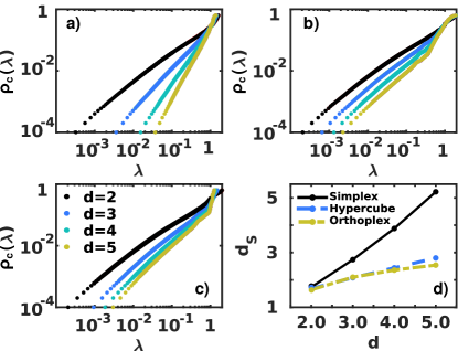
Figure 1: The cumulative distribution of eigenvalues $\rho_{c}(\lambda)$ for CNM of dimension $d=2,\ 3,\ 4$ and $5$, is shown in panels $(a)$, $(b)$ and $(c)$ for the simplex, hypercube and orthoplex CNM respectively. Panel $(d)$ represents the fitted spectral dimension of the CNM as a function of the dimension $d$ of its building blocks. Results are for $N=6400$ and the cumulative distribution of eigenevalue $\rho_{c}(\lambda)$ is averaged over $100$ realizations of the network.

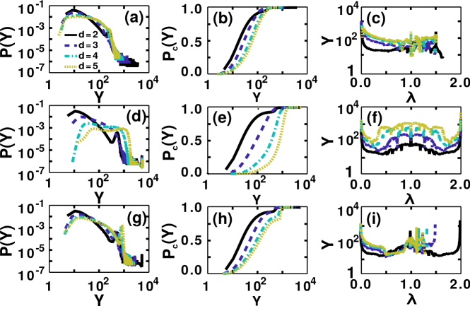
Figure 2: The probability distribution $P(Y)$, the cumulative distribution $P_{c}(Y)$ of the participation ratio $Y$, and the average value of the participation ratio $Y$ as a function of the corresponding eigenvalue $\lambda$ are shown for CNM formed by simplices (panels $(a,b,c)$), hypercubes (panels $(d,e,f)$) and orthoplexes (panels $(g,h,i)$) networks with dimension $d=2,3,4,5$ of the polytopes.

IV Kuramoto dynamics on networks with finite spectral dimension

IV.1 The Kuramoto model

Synchronization dynamics on complex networks has been widely studied in the literature and it is known to be very significantly affected by the spectral properties of the network. However, the scientific interest so far has focused on networks which do not have a spectral dimension and display instead what is called a spectral gap, i.e. the smallest non-zero eigenvalue of the normalized Laplacian $\lambda_{2}$ does not approaches zero in the infinite network limit.

However, in network geometries it is important to consider network structures in which the spectral gap closes, $\lambda_{2}\to 0$ as $N\to\infty$, and the density of eigenvalues follows the scaling in Eq. (11), i.e. the network has a finite spectral dimension. To investigate the role of the spectral dimension in the synchronization dynamics, we consider the Kuramoto model.

The Kuramoto dynamics describes a system of $N$ coupled oscillators $i=1,2,\ldots,N$ with phases $\theta_{i}(t)$ obeying the following dynamical equation,

$$\dot{\theta}_{i}(t)=\omega_{i}+\sigma\sum_{j=1}^{N}\frac{a_{ij}}{k_{i}}\sin(\theta_{j}-\theta_{i}),$$ (27)

where $k_{i}$ is the degree of node $i$, $a_{ij}$ the adjacency matrix of the network, and $\sigma$ the control parameter tuning the strength of the coupling between nodes. Each internal frequency $\omega_{i}$ is independently drawn from a normal distribution with mean $0$ and variance $1$, i.e. ${\mathcal{N}}(0,1).$ We note that sometimes the Kuramoto model is defined by omitting $k_{i}$ in Eq. (27), however our choice here is dictated by the desire to screen out the effect of having heterogeneous degree distributions. Therefore, the considered dynamics is designed to be independent of the degree distribution so that the effect of having networks with different spectral dimension can be revealed.

IV.2 Theoretical predictions

In order to study the stability of the synchronized phase, we have linearized the Kuramoto dynamics in Eq. $(\ref{Kuramoto})$ assuming that $|\theta_{i}-\theta_{j}|\ll 1$ for every pair of neighbour nodes. In this way we get the linear system of equations

$$\dot{\theta}_{i}(t)=\omega_{i}-\sigma\sum_{j=1}^{N}{L}_{ij}\theta_{j},$$ (28)

for $i=1,2,\ldots,N$, where $\bf{L}$ is defined in Eq. (1). In order to evaluate the stability of the synchronized state, we use an approach already established for finite lattices Choi ; Chate . Specifically we calculate the average fluctuation of the phases over the entire network by evaluating $W^{2}$ given by

$$W^{2}=\frac{1}{N}\left\langle{\sum_{i=1}^{N}[\theta_{i}(t)-\overline{\theta}]^{2}}\right\rangle,$$ (29)

where in Eq. (29) $\overline{\theta}$ is given by

$$\overline{\theta}=\frac{1}{N}\sum_{i=1}^{N}{\theta_{i}(t)},$$ (30)

in the linear approximation. In presence of a thermodynamically stable synchronized phase, the average fluctuations of the phases $W^{2}$ should remain bounded. Therefore, if $W^{2}$ diverges with the network size $N$, the synchronized phase is unstable. By considering networks having a finite spectral dimension $d_{S}$ we obtain (see Appendix A) that in the large network limit ($N\to\infty$) $W^{2}$ diverges as long as $d_{S}\leq 4$. Specifically we can show that $W^{2}$ obeys the scaling

$$W^{2}\sim\left\{\begin{array}[]{ll}N^{4/{d}_{S}-1}&\mbox{if }{d}_{S}<4,\\ \ln(N)&\mbox{if }{d}_{S}=4,\\ \mbox{const}&\mbox{if }{d}_{S}>4.\end{array}\right.$$ (34)

It follows from this derivation that the synchronized state cannot be thermodynamically stable in networks with spectral dimension $d_{S}\leq 4$.

The linear approximation is valid only if the coupling term of each oscillator with the phases of the linked oscillators is small. Therefore in order for the linear approximation to hold we must require that the vector ${\bf L}\bm{\theta}$ has small elements. A global parameter that can establish the sufficient condition for the failure of the linear approximation is the correlation $C$ defined as

$$C=\frac{1}{N}\left\langle{\bm{\theta}^{T}{\bf L}\bm{\theta}}\right\rangle.$$ (35)

In fact, if the correlation $C$ diverges the linear approximation cannot be valid. In a network with finite spectral dimension $d_{S}$ we have obtained (see detailed derivation in Appendix B) that $C$ obeys the following scaling with $N$,

$$C\sim\left\{\begin{array}[]{ll}N^{2/{d}_{S}-1}&\mbox{if }{d}_{S}<2,\\ \ln(N)&\mbox{if }{d}_{S}=2,\\ \mbox{const}&\mbox{if }{d}_{S}>2.\end{array}\right.$$ (39)

Therefore, for spectral dimension $d_{S}\leq 2$ the correlations among the phases of nearest neighbour nodes diverge and the linear approximation fails.

So far we have shown that for spectral dimension $d_{S}<2$ the linear approximation fails, while for spectral dimensions $d_{S}\in(2,4]$ the linear approximation can be valid but the synchronized phase is not thermodynamically stable. In order to uncover the phenomenology for spectral dimensions $d_{S}\in(2,4]$, we follow the approach used by Choi ; Chate for regular lattices. We start by characterizing the fluctuations observed in phase velocities across the nodes of the network

$$V^{2}=\frac{1}{N}\sum_{i=1}^{N}\left\langle{\left[{\psi}_{i}-\bar{\psi}\right]^{2}}\right\rangle,$$ (40)

where $\psi_{i}$ indicates the phase velocity of node $i$,

$$\psi_{i}=\dot{\theta_{i}},$$ (41)

and $\bar{\psi}$ the average of the phase velocities over the network

$$\bar{\psi}=\frac{1}{N}\sum_{i=0}^{N}\psi_{i}.$$ (42)

In Appendix C we show that, as long as the linear approximation is valid, i.e. $d_{S}>2$, the fluctuations observed in phase velocities vanish in the large network limit, i.e.

$$V^{2}\to 0 N\to\infty.$$ as (43)

This analysis therefore reveals that for spectral dimensions $d_{S}\in(2,4]$ phase entrainment takes place as long as the linear approximation is valid.

V Kuramoto model on Complex Network Manifolds

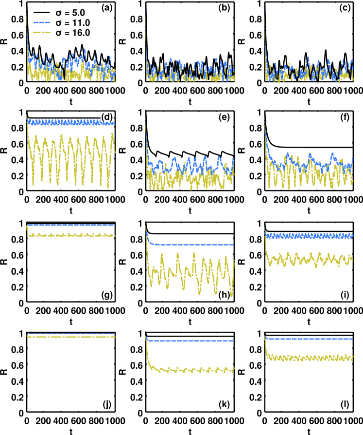
Figure 3: Time series of the global order parameter calulcated for different values of $\sigma=5$, $11$ and $16$, as indicated in the legend, and for CNM formed by simplices (panels $(a)$, $(d)$, $(g)$, $(j)$), hypercubes (panels $(b)$, $(e)$, $(h)$, $(k)$) and orthoplex (panels $(c)$, $(f)$, $(i)$, $(l)$) of dimensions $d=2$ (panels $(a)$, $(b)$, $(c)$), $d=3$ (panels $(d)$, $(e)$, $(f)$), $d=4$ (panels $(g)$, $(h)$, $(i)$) and $d=5$ (panels $(j)$, $(k)$, $(l)$).

In this section we present numerical results of the Kuramoto dynamics defined over CNM. As CNM have tunable spectral dimension this analysis will provide a solid benchmark where we can test our theoretical predictions. The macroscopic state of synchronization of the system at each time $t$ is characterized by the Kuramoto order parameter, defined as

$$Z(t)=R(t)e^{i\phi(t)}=\frac{1}{N}\sum_{j=1}^{N}e^{i\theta_{j}(t)},$$ (44)

where $R(t)\in\left[0,1\right]$ is a real variable that quantifies the level of global synchronization, and $\phi(t)$ gives the average global phase of collective oscillations Kurths ; kuramoto1975self . Therefore, $R(t)\approx 0$ corresponds to the noisy or non-coherent state, whereas $R(t)\approx 1$ corresponds to the coherent or synchronized state.

We simulated the Kuramoto dynamics by integrating the system of Eqs. (27) in MATLAB using the ode45 function, which uses a non-stiff $4$-th order integration algorithm with adaptive time steps. Simulations are run for a total time $T$, and for different realizations of the CNM, formed by $d$-dimensional simplices, hypercubes and orthoplexes.

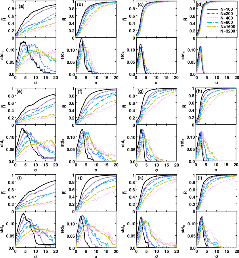
Figure 4: The average order parameter $\bar{R}$ and the standard deviation of the order parameter $std_{R}$) are plotted versus the coupling constant $\sigma$ for CNM formed by simplices (panels $(a)$, $(b)$, $(c)$, $(d)$), hypercubes (panels $(e)$, $(f)$, $(g)$, $(h)$) and orthoplexes (panels $(i)$, $(j)$, $(k)$, $(l)$) and for dimension $d=2$ (panels $(a)$, $(e)$, $(i)$), $d=3$ (panels $(b)$, $(f)$, $(j)$), $d=4$ (panels $(c)$, $(g)$, $(k)$) and $d=5$ (panels $(d)$, $(h)$, $(l)$). Results are shown for different network sizes $N=100,\ 200,\ 400,\ 800,\ 1600$ and $3200$ as indicated in the legend. Results are for $T=1000$ and have been averaged after equilibration for $20$ realizations of the networks and internal frequencies.

Our numerical analysis reveals that CNM can display a frustrated synchronization phase with fully entrained phases in which the global order parameter $R(t)$ has large temporal fluctuations. The typical range of values of the coupling constants where we observe this phase depends both on the spectral dimension $d_{S}$ and the network size $N$. In Figure 3 we show single instances of the time series $R(t)$ of the global order parameter defined on CNM of size $N=3200$ for representative values of the coupling $\sigma$ and for different polytopes and dimensions. Characteristic states of frustrated synchronization can be observed for $\sigma=5.0$ and $d=3,4$ for CNM formed by simplex, hypercubes and orthoplex (panels $(d)$, $(e)$, $(f)$, $(g)$, $(h)$ and $(i)$ of Figure ${fig:series}$); and also for $d=5$ for CNM formed by hypercubes and orthoplex (panels $(k)$ and $(l)$ for Figure 3).

In general, for CNM formed by a finite number of nodes $N$, as the coupling constant $\sigma$ increases we can generally distinguish between three phases. For very small values of the coupling constant $\sigma$, the order parameter $R(t)\approx 0$, i.e. the oscillators are not coherent (as shown for example in panels $(a)$ and $(b)$ of Figure 3). For large values of the coupling constant $\sigma$ we observe a synchronized phase and a stationary time-series of $R(t)$ with large values of $R(t)$ (see for instance curves obtained for $\sigma=11.0$, and $\sigma=16.0$, in panels $(a)$ and $(b)$ of Figure 3). In the intermediate range of values of the coupling constant $\sigma$, we observe the frustrated synchronization regime of phase entrainment where the order parameter $R(t)$ is not stationary (see for instance curves obtained for $\sigma=5.0$ in panels $(d)$, $(e)$ and $(f)$ of Figure 3).

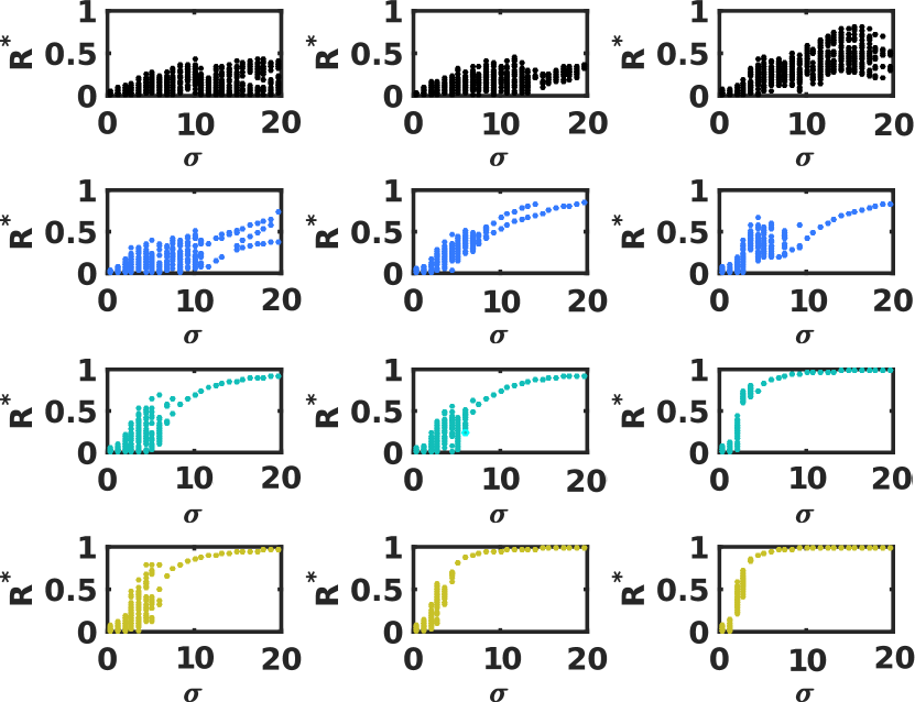
Figure 5: Orbit diagrams of the system dynamics for CNM formed by simplices (left panels), hypercubes (center panels) and orthoplexes (right panel) for $d=2,\ 3,\ 4$ and $5$ from top to bottom. The orbit diagrams are represented by the extremes (maxima and minima) $R^{*}$ taken by $R(t)$ for $t>0.8T$. Results are for $N=3200$, $T=1000$ and a given realization of the networks structure.

In order to investigate the thermodynamical stability of these phases in the large network limit as a function of the spectral dimension $d_{S}$, we have studied the finite size effects of the Kuramoto synchronization for CNM formed by simplices, hypercubes and orthoplexes for dimensions $d=2,3,4,5$. The spectral dimension of these CNM is shown in Figure 1. For $d=2$ CNM have spectral dimension $d_{S}\approx 2$, whereas for $2<d\leq 5$ CNM formed by simplices have spectral dimension $d_{S}$ that in first approximation can be assumed to be $d_{S}\approx d$ and CNM formed by hypercubes and orthoplexes have spectral dimension $d_{S}\in(2,3)$. Consequently, our theoretical expectation is that for $d=2$ we cannot observe entrained phases, and that for $2<d\leq 4$ we can observe entrained phases and the synchronized phase cannot be thermodynamically stable. Moreover for $d=5$ our predictions are that CNM formed by simplices can display a thermodynamically stable synchronized phase while CNM formed by hypercubes and orthoplexes cannot display a thermodynamically stable synchronized phase.

In order to test these predictions we have numerically studied as functions of the coupling $\sigma$ the mean value $\bar{R}$ and the standard deviation $std_{R}$ of the order parameter $R(t)$, averaged after the transient evolution over different realizations of CNM. In Figure 4 we display $\bar{R}$ and $std_{R}$ for CNM formed by simplices, hypercubes and orthoplex of dimension $d=2,3,4,5$ and different network sizes $N$. The de-coherent or unsynchronized phase corresponds to the regime where $\bar{R}$ is low. The synchronized phase corresponds to the regime where $\bar{R}$ is high and the fluctuations $std_{R}$ are low. Finally, the frustrated synchronization phase corresponds to values of the coupling where both $\bar{R}$ and $std_{R}$ have significantly high values. As the network size $N$ increases we observe different scenarios depending on the value of the spectral dimension $d_{S}$. For spectral dimension $d_{S}\approx 2$, in the large network limit the system remains in the de-coherent state. This occurs for all considered CNM of dimension $d=2$. For spectral dimension $d_{S}\in(2,4]$, we observe that the synchronized phase is not thermodynamically stable as the values of coupling constant where the onset of this phase is observed increase with the network size and do not converge to a finite value. It occurs for CNM formed by simplices of dimension $d=3,4$ and for CNM formed by hypercubes and orthoplexes of dimension $d=3,4,5$. Finally, for spectral dimension $d_{S}>4$ we observe that the synchronized phase is thermodynamically stable as the onset of this phase occurs at a finite value of $\sigma$ in the large network limit.

In summary, our numerical study of the synchronization properties of CNM indicates that the phase diagram of the model depends critically on the spectral dimension $d_{S}$ as predicted by our theoretical investigation.

The properties of the frustrated synchronization phase observed in CNM are here furthermore investigated by means of the orbit diagrams Poincare (see Figure 5). These are measured as the extrema $R^{*}$ (maximum and minimum) of the time series $R(t)$ for each coupling $\sigma$. Therefore, a fixed stationary state is represented by one point corresponding to the mean value, as it appears in the synchronized state observed for high values of $\sigma$ provided that $d>2$. This situation corresponds to one of full synchronization if $R^{*}=1$ or to partial synchronization if $R^{*}<1$, in which some nodes remain unsynchronized. For spectral dimensions $d_{S}\in(2,4]$, on the other hand, we observe that, as the value of the coupling constant $\sigma$ is lowered and we enter in the frustrated synchronization phase, oscillatory states appear with a given number of extrema that depends on the network and frequency realization. These typically correspond to intereference among different locally synchronized regions, whose sizes scale as $N$ Ana , which gives rise to a chaotic behavior as the coupling constant $\sigma$ is decreased. Finally, in the case $d_{S}\approx d=2$ the synchronized state is never reached.

VI Conclusions

This work investigates the role of the spectral dimension $d_{S}$ on the synchronization properties of the Kuramoto model. Using a linear approximation we have shown that the synchronized phase cannot be thermodynamically stable for spectral dimension $d_{S}\leq 4$. Therefore a necessary condition to observe a synchronized regime in the thermodynamic limit is that $d_{S}>4$. We have also shown that the considered linear approximations cannot be valid for $d_{S}\leq 2$, since the correlations $C$ diverge. Finally, we have shown that, for spectral dimension $d_{S}\in\left(2,4\right]$, phase entrainment takes place in the large network limit as long as the linear approximation is valid, i.e. the fluctuations in phase velocities, $V^{2}$, vanish asymptotically in time, so that the phases of the nodes are totally entrained.

In order to consider a concrete example where to test these theoretical derivations, we have characterized the synchronization dynamics of the normalized Kuramoto model taking place on Complex Network Manifolds which have a tunable spectral dimension. These networks define discrete manifolds with the small-world property (infinite Hausdorf dimension) and highly modular structure, and provide an ideal theoretical setting to explore the interplay between network geometry and synchronization dynamics Ana .

CNM have significant spectral properties and display a finite spectral dimension. In particular, we have found that CNM based on simplicial complexes have a spectral dimension $d_{S}$ increasing almost linearly with the dimension $d$ of the simplices, whereas CNM formed by $d$-dimensional hypercubes and orthoplexes have a spectral dimension $d_{S}$ that saturates with $d$. Having a tunable spectral dimension, CNM can be compared to Euclidean lattices that have a spectral dimension $d_{S}$ equal to their Hausdorff dimension, i.e. $d_{S}=d_{H}$. However, CNM have a hyperbolic structure with $d_{H}=\infty$ and we always observe $d_{S}<d_{H}$. Moreover, a closer look at the localization properties of the eigenvectors CNM reveals more significant differences with respect to Euclidean lattices. In fact, contrarily to the Fourier eigenvector of Euclidean lattices, a large fraction of eigenmodes of CNM are highly localized on few nodes of the network, reflecting the symmetries of the building block structure.

We have studied numerically the Kuramoto dynamics on CNM testing our theoretical predictions on the nature of the synchronization dynamics as a function of the spectral dimension $d_{S}$. We show that a frustrated synchronization regime with entrained phases emerges for spectral dimensions $d_{S}\in(2,4]$ and that, for this range of values of the spectral dimension, finite CNM with high coupling constant $\sigma$ reach also a synchronized phase but this phase is not thermodynamically stable. Moreover, we show that for spectral dimension $d_{S}=5$ the synchronized phase is thermodynamically stable.

In conclusion our work reveals that non-trivial synchronization states can emerge even in small-world networks, with an infinite Hausdorff dimension, provided that the spectral dimension is finite. These results reveal deep connections between geometry and synchronization dynamics and are potentially very useful to further investigate the relation between structural and functional brain networks.

Appendix A Stability of the synchronized phase

In this Appendix we will investigate the stability of the synchronized phase by considering the linearized dynamical system given by Eqs. (28). The normalized Laplacian ${\bf{L}}$ appearing in Eqs. (28) and defined in Eq. (1) is diagonalizable with eigenvalues $\{\lambda_{i}\}_{i=1,2,\ldots,N}$, numbered in increasing order, $0=\lambda_{1}<\lambda_{2}\leq\lambda_{3},\ldots,\leq\lambda_{N}$, and therefore can be written as

$$\bf{P}^{-1}{L}P=D,$$ (45)

where ${\bf P}$ is the matrix whose columns are the right eigenvectors ${\bf v}^{\lambda}$ and and ${\bf P}^{-1}$ is the matrix whose rows are the left eigenvectors ${\bf u}^{\lambda}$ of ${\bf{L}}$. Notice that we always have ${\bf P}^{-1}{\bf P}={\bf I}$, where ${\bf I}$ indicates the identity matrix, due to the normalization condition of the eigenvectors given by Eq. (9).

The vector $\bm{\theta}=\left(\theta_{1},\theta_{2},\ldots,\theta_{N}\right)^{T}$ can be projected in the base of the right and left eigenvectors, so $\theta_{i}$ can be equivalently expressed as

$$\theta_{i} = \sum_{\lambda}\theta_{\lambda}^{R}v_{i}^{\lambda},$$

$$\theta_{i} = \sum_{\lambda}\theta_{\lambda}^{L}u_{i}^{\lambda},$$ (46)

or, equivalently,

$$\bm{\theta} = {\bf P}\bm{\theta}^{R},$$

$$\bm{\theta} = [{\bf P}^{-1}]^{T}{\bm{\theta}}^{L},$$ (47)

where we have indicated with $\bm{\theta}^{R}$ and $\bm{\theta}^{L}$ the column vector of elements $\theta_{\lambda}^{R}$ and $\theta_{\lambda}^{L}$, respectively. Inverting these relations we have that $\bm{\theta}^{R}$ and $\bm{\theta^{L}}$ are given by

$${\bm{\theta}}^{R} = {\bf P}^{-1}{\bm{\theta}},$$

$${\bm{\theta}}^{L} = {\bf P}^{T}{\bm{\theta}}.$$ (48)

Similarly we can also consider the vector $\bm{\omega}$ of elements $\omega_{i}$ and project it along the bases of the right and the left eigenvectors,

$$\bm{\omega} = {\bf P}\bm{\omega}^{R},$$

$$\bm{\omega} = [{\bf P}^{-1}]^{T}{\bm{\omega}}^{L}.$$ (49)

Inverting these relations we obtain

$${\bm{\omega}}^{R} = {\bf P}^{-1}{\bm{\omega}},$$

$${\bm{\omega}}^{L} = {\bf P}^{T}{\bm{\omega}}.$$ (50)

The linearized Eq. $(\ref{linearized})$ can also be projected along the bases of right and left eigenvectors getting

$$\frac{d\theta^{R}_{\lambda}}{dt} = \omega^{R}_{\lambda}-\sigma\lambda\theta^{R}_{\lambda},$$

$$\frac{d\theta^{L}_{\lambda}}{dt} = \omega^{L}_{\lambda}-\sigma\lambda\theta^{L}_{\lambda}.$$ (51)

This equations can be solved obtaining, for $\lambda\neq 0$,

$$\theta_{\lambda}^{R/L}(t)=e^{-\sigma\lambda t}\theta_{\lambda}^{R/L}(0)+\frac{\omega_{\lambda}^{R/L}}{\sigma\lambda}(1-e^{-\sigma\lambda t}),$$ (52)

and, for $\lambda=0$,

$$\theta_{\lambda}^{R/L}(t)=\theta_{\lambda=0}^{R/L}(0)+{\omega_{\lambda=0}^{R/L}}t.$$ (53)

Finally, let us note that $\bm{\omega}^{R,L}$ have the following averages

$$\left\langle{\omega^{R,L}_{\lambda}}\right\rangle = 0.$$

$$\left\langle{\omega^{R}_{\lambda}\omega^{L}_{\lambda^{\prime}}}\right\rangle = \sum_{i=1}^{N}\sum_{j=1}^{N}\left\langle{\omega_{i}\omega_{j}}\right\rangle u_{i}^{\lambda}v_{j}^{\lambda^{\prime}}=\delta_{\lambda,\lambda^{\prime}}.$$ (54)

As mentioned in the main text, in order to evaluate the stability of the synchronized state, we use an approach already established for finite lattices Choi ; Chate and we calculate the average fluctuation of the phases over the entire network. These fluctuations are quantified by $W^{2}$ given by

$$W^{2}=\frac{1}{N}\left\langle{\sum_{i=1}^{N}[\theta_{i}(t)-\overline{\theta}]^{2}}\right\rangle,$$ (55)

where

$$\overline{\theta}=\frac{1}{N}\sum_{i=1}^{N}{\theta_{i}(t)}.$$ (56)

The divergence of $W^{2}$ with the network size $N$ will indicate that the synchronized phase is unstable.

Since $\bm{\theta}$ can be expressed equivalently in the base of right and left eigenvectors as expressed in Eqs. $(\ref{theta_eigenvectors})$, and the right eigenvector is given by the first of Eqs. $(\ref{eigen})$, we can calculate $\overline{\theta}$ in terms of $\bm{\theta}^{L}$ and $\bm{\theta}^{R}$ as

$$\overline{\theta} = \sqrt{\frac{\langle{k}\rangle}{N}}{\theta}_{\lambda=0}^{L}(t)$$

$$\overline{\theta} = \sum_{\lambda}\theta_{\lambda}^{R}(t)\frac{1}{N}\sum_{i}{v}_{i}^{\lambda}$$ (57)

Using the explicit solution of $\theta^{L}_{\lambda}(t)$ and $\theta^{R}_{\lambda}(t)$ given by Eq. (52) and Eq. $(\ref{sol0})$ and using Eqs. (54) we can express $\left\langle{\overline{\theta}^{2}}\right\rangle$ as

$$\left\langle{\overline{\theta}^{2}}\right\rangle = \frac{1}{N}\left\langle{\theta_{\lambda=0}^{L}(t)\theta_{\lambda=0}^{R}(t)}\right\rangle+\sqrt{\frac{\langle{k}\rangle}{N}}\theta_{\lambda=0}^{L}(0)\theta_{\lambda=0}^{R}(0)$$ (58)

$$\times\sum_{\lambda\neq 0}e^{-\sigma\lambda t}\frac{1}{N}\sum_{i=1}^{N}v_{i}^{\lambda}.$$

Therefore asymptotically in time, for $t\to\infty$, we obtain

$$\left\langle{\overline{\theta}^{2}}\right\rangle=\frac{1}{N}\left\langle{\theta_{\lambda=0}^{L}(t)\theta_{\lambda=0}^{R}(t)}\right\rangle.$$ (59)

The fluctuations of the phases of the Kuramoto dynamics can be evaluated by considering that $W^{2}$ can be equivalently expressed as

$$W^{2}=\frac{1}{N}\left\langle{\bm{\theta}^{T}\bm{\theta}}\right\rangle-\left\langle{\overline{\theta}^{2}}\right\rangle.$$ (60)

Using Eq. (48) we note that $\left\langle{\bm{\theta}^{T}\bm{\theta}}\right\rangle$ has a simple expression in terms of $\bm{\theta}^{L}$ and $\bm{\theta}^{R}$, i.e.

$$\left\langle{\bm{\theta}^{T}\bm{\theta}}\right\rangle=\left\langle{[\bm{\theta}^{L}]^{T}{\bf P^{-1}}{\bf P}[\bm{\theta}^{R}]}\right\rangle=\left\langle{[\bm{\theta}^{L}]^{T}\bm{\theta}^{R}}\right\rangle.$$ (61)

Using the solution of the Kuramoto dynamics Eq. $(\ref{soln})$ and Eqs. (54) we get

$$\left\langle{[\bm{\theta}^{L}]^{T}\bm{\theta}^{R}}\right\rangle=\left\langle{\theta_{\lambda=0}^{L}(t)\theta_{\lambda=0}^{R}(t)}\right\rangle$$

$$+\sum_{\{\lambda\}|\lambda\neq 0}\left[e^{-2\sigma\lambda t}\theta_{\lambda}^{R}(0)\theta_{\lambda}^{L}(0)+\frac{1}{(\sigma\lambda)^{2}}(1-e^{-\sigma\lambda t})^{2}\right].$$ (62)

Finally using Eq. $(\ref{zero})$ together with Eqs. (59)-(62), it results that asymptotically in time for $t\to\infty$

$$W^{2}=\int_{\lambda_{2}}^{\lambda_{max}}d\lambda\rho(\lambda)\frac{1}{(\sigma\lambda)^{2}}.$$ (63)

Since the Fidler eigenvalue $\lambda_{2}$ satisfies the scaling expressed in Eq. $(\ref{Fidler})$ and goes to zero in the infinite network limit, using the scaling in Eq. (11) for the density of eigenvalues $\rho(\lambda)$ we obtain the following results.

• For spectral dimension $d_{S}<4$ the average fluctuation of the phases $W^{2}$ diverges as

  $$W^{2}\simeq O\left(\lambda_{2}^{d_{S}/2-2}\right)$$ (64)

• For spectral dimension $d_{S}=4$ the average fluctuation of the phases $W^{2}$ diverges as

  $$W^{2}\simeq O(-\ln\lambda_{2}).$$ (65)

• Only for spectral dimension $d>4$ the average fluctuation of the phases $W^{2}$ converges.

Specifically, by inserting the scaling of the Fidler eigenvalue Eq. $(\ref{Fidler})$ with the network size $N$ we obtain

$$W^{2}\sim\left\{\begin{array}[]{ll}N^{4/{d}_{S}-1}&\mbox{if }{d}_{S}<4\\ \ln(N)&\mbox{if }{d}_{S}=4\\ \mbox{const}&\mbox{if }{d}_{S}>4.\end{array}\right.$$ (69)

It follows from this derivation that the synchronized state cannot be thermodynamically stable in networks with spectral dimension $d_{S}\leq 4$.

Appendix B Correlations between phases and validity of the linear approximation

In this Appendix we will evaluate the scaling of the correlation $C$ defined as

$$C=\frac{1}{N}\left\langle{\bm{\theta}^{T}{\bf L}\bm{\theta}}\right\rangle$$ (70)

in the linear approximation. The divergence of the correlation $C$ in the large network limit indicates that the linear approximation fails to be valid. The correlation can be expressed in the basis of eigenvalues of the normalized Laplacian getting the simple expression

$$C=\frac{1}{N}\sum_{\lambda}\left\langle{\theta_{\lambda}^{L}\lambda\theta_{\lambda}^{R}}\right\rangle.$$ (71)

By using the explicit expression for $\theta_{\lambda}^{L/R}$ given by Eq. $(\ref{soln})$ it is easy to show that

$$C = \frac{1}{N}\sum_{\{\lambda\}|\lambda\neq 0}\lambda\left[e^{-2\sigma\lambda t}\theta_{\lambda}^{R}(0)\theta_{\lambda}^{L}(0)+\frac{1}{(\sigma\lambda)^{2}}(1-e^{-\sigma\lambda t})^{2}\right]$$

which gives in the asymptotic limit $t\to\infty$

$$C = \int_{\lambda_{2}}^{\lambda_{N}}\rho(\lambda)\frac{1}{\sigma^{2}\lambda}d\lambda.$$ (72)

By inserting the scaling of the Fidler eigenvalue with the network size $N$ given by Eq. $(\ref{Fidler})$ we obtain

$$C\sim\left\{\begin{array}[]{ll}N^{2/{d}_{S}-1}&\mbox{if }{d}_{S}<2\\ \ln(N)&\mbox{if }{d}_{S}=2\\ \mbox{const}&\mbox{if }{d}_{S}>2.\end{array}\right.$$ (76)

Therefore, for spectral dimension $d_{S}\leq 2$ the correlations among the phases of nearest neighbour nodes diverge and the linear approximation fails.

Appendix C Entrained phases

In this Appendix we will characterize the fluctuations observed in phase velocities across the nodes of the network quantified by the global parameter $V^{2}$ given by

$$V^{2}=\frac{1}{N}\sum_{i=1}^{N}\left\langle{\left[{\psi}_{i}-\bar{\psi}\right]^{2}}\right\rangle$$ (77)

where $\psi_{i}$ indicates the phase velocity of node $i$

$$\psi_{i}=\dot{\theta_{i}},$$ (78)

and $\bar{\psi}$ the average of the phase velocities over the network

$$\bar{\psi}=\frac{1}{N}\sum_{i=0}^{N}\psi_{i}.$$ (79)

The phase velocities $\bm{\psi}=(\psi_{1},\psi_{2},\ldots,\psi_{N})^{T}$ can be projected into the basis of right and left eigenvectors of the normalized Laplacian getting

$${\bm{\psi}}^{R} = {\bf P}^{-1}{\bm{\psi}},$$

$${\bm{\psi}}^{L} = {\bf P}^{T}{\bm{\psi}}.$$ (80)

By using the solution of the linearized dynamics, Eqs. (52) and $(\ref{sol0})$, it is easy to show that with the linear approximation we have

$$\psi_{\lambda}^{R/L}(t)=\dot{\theta_{\lambda}}^{R/L}=-\sigma\lambda e^{-\sigma\lambda t}\theta_{\lambda}^{R/L}(0)+{\omega_{\lambda}^{R/L}}e^{-\sigma\lambda t},$$ (81)

and for $\lambda=0$

$$\psi_{\lambda}^{R/L}(t)={\omega_{\lambda=0}^{R/L}}.$$ (82)

Using the same procedure used previously for the derivation of $\bar{\theta}$, it is easy to show that the average phase velocity $\bar{\psi}$ can be expressed equivalently as

$$\bar{\psi} = \sqrt{\frac{\langle{k}\rangle}{N}}{\psi}_{\lambda=0}^{L}(t),$$

$$\bar{\psi} = \sum_{\lambda}\psi_{\lambda}^{R}(t)\frac{1}{N}\sum_{i}{v}_{i}^{\lambda}.$$ (83)

From these expressions, and using Eqs. (54), it follows that

$$\left\langle{\bar{\psi}^{2}}\right\rangle=\frac{1}{N}\left\langle{{\psi}_{\lambda=0}^{L}(t){\psi}_{\lambda=0}^{r}(t)}\right\rangle.$$ (84)

Finally using again Eq. (54) we get that

$${V^{2}} = \frac{1}{N}\left\langle{[{\bm{\psi}^{L}}]^{T}{\bm{\psi}}^{R}}\right\rangle-\left\langle{\bar{\psi}^{2}}\right\rangle$$ (85)

scales in the asymptotic limit $t\to\infty$ as

$$V^{2} \sim \int_{\lambda_{2}}^{\lambda_{max}}d\lambda\rho(\lambda)e^{-2\sigma\lambda t}$$ (86)

$$\sim t^{-d_{S}/2}.$$

This result implies that asymptotically in time the fluctuations in the phase velocities vanish, i.e.

$$V^{2}\to 0$$ (87)

as $t\to\infty$. This result implies that the phases of the oscillators are totally entrained as long as the linear approximation is valid.

References

- (1) G. Bianconi, Interdisciplinary and physics challenges of network theory, EPL (Europhysics Letters) 111, 56001 (2015).
- (2) C. Giusti, R. Ghrist and D. S. Bassett, Two’s company, three (or more) is a simplex, J. Computational Neuroscience, 41, 1 (2016).
- (3) Salnikov, Vsevolod, D. Cassese, and R. Lambiotte, Simplicial complexes and complex systems. arXiv preprint arXiv:1807.07747 (2018).
- (4) Z. Wu, G. Menichetti, C. Rahmede and G. Bianconi, Emergent complex network geometry, Sci. Rep. 5, 10073 (2014).
- (5) G. Bianconi and C. Rahmede, Complex quantum network manifolds in dimension are scale-free, Sci. Rep. 5, 13979 (2015).
- (6) G. Bianconi and C. Rahmede, Network geometry with flavor: from complexity to quantum geometry, Phys. Rev. E 93, 032315 (2016).
- (7) G. Bianconi and C. Rahmede, Emergent hyperbolic network geometry, Sci. Rep. 7 41974 (2017).
- (8) D. Mulder and G. Bianconi, Network Geometry and Complexity J. Stat. Phys. (2018).
- (9) D. C. da Silva, G. Bianconi, R. A. da Costa, S. N. Dorogovtsev, and J. F. F. Mendes, Complex network view of evolving manifolds, Phys. Rev. E 97, 032316 (2018).
- (10) M. Boguñá, F. Papadopoulos, and D. Krioukov, Sustaining the internet with hyperbolic mapping, Nature Commun. 1, 62 (2010).
- (11) D. Krioukov, F. Papadopoulos, M. Kitsak, A. Vahdat, and M. Boguñá., Hyperbolic geometry of complex networks, Phys. Rev. E 82, 036106 (2010).
- (12) J. Jost, and S. Liu, Ollivier’s Ricci curvature, local clustering and curvature-dimension inequalities on graphs, Discrete & Computational Geometry 51, 300 (2014).
- (13) A. Muscoloni, J. M. Thomas, S. Ciucci, G. Bianconi and C. V. Cannistraci, Machine learning meets complex networks via coalescent embedding in the hyperbolic space. Nature Communications, 8, 1615 (2017).
- (14) M. M. Bronstein, J. Bruna, Y. LeCun, A. Szlam and P. Vandergheynst, Geometric deep learning: going beyond euclidean data. IEEE Signal Processing Magazine, 34, 18 (2017).
- (15) G. Petri, P. Expert, F. Turkheimer, R. Carhart-Harris, D. Nutt, P. J. Hellyer, and F. Vaccarino, Homological scaffolds of brain functional networks, J. Royal Society Interface 11, 20140873 (2014).
- (16) M. W. Reimann, M. Nolte, M. Scolamiero, et al., Cliques of neurons bound into cavities provide a missing link between structure and function, Front. Comp. Neuro. 11, 48 (2017).
- (17) V. Salnikov, D. Cassese, R. Lambiotte, and N. S. Jones, Co-occurrence simplicial complexes in mathematics: identifying the holes of knowledge, arXiv preprint arXiv:1803.04410 (2018).
- (18) M. Šuvakov, M. Andjelković, and B. Tadić, Hidden geometries in networks arising from cooperative self-assembly, Sci. Rep. 8, 1987 (2018).
- (19) J. R. Clough, and T.S. Evans, Embedding graphs in Lorentzian spacetime, PloS one, 12, e0187301 (2017).
- (20) M. Tumminello, T. Aste, T. Di Matteo and R. N. Mantegna, A tool for filtering information in complex systems, Proc. Nat. Aca. Sci., 102 10421 (2005).
- (21) W. Barfuss, G. P. Massara, T. Di Matteo and T. Aste, Parsimonious modeling with information filtering networks, Phys. Rev. E, 94, 062306 (2016).
- (22) J. Ambjorn, J. Jurkiewicz and R. Loll, Reconstructing the universe, Phys. Rev. D 72, 064014 (2005).
- (23) D. Oriti, Spacetime geometry from algebra: spin foam models for non-perturbative quantum gravity, Reports on Progress in Physics 64, 1703 (2001).
- (24) L. Lionni, Colored discrete spaces: Higher dimensional combinatorial maps and quantum gravity, arXiv preprint arXiv:1710.03663 (2017).
- (25) A. P. Millán, J. J. Torres and G. Bianconi, Complex Network Geometry and Frustrated Synchronization, Sci. Rep.8, 9910 (2018).
- (26) G. Petri and A. Barrat, Simplicial Activity Driven Model, arXiv preprint arXiv:1805.06740 (2018).
- (27) I. Iacopini, G. Petri, A. Barrat and V. Latora, Simplicial models of social contagion. arXiv preprint arXiv:1810.07031 (2018).
- (28) R. Rammal, and G. Toulouse, Random walks on fractal structures and percolation clusters, Journal de Physique Lettres, 44, 1 (1983).
- (29) R. Burioni, and D. Cassi, Random walks on graphs: ideas, techniques and results. Jour. Phys. A 38, R45 (2005).
- (30) R. Burioni and D. Cassi, Universal properties of spectral dimension, Phys. Rev. Lett., 76, 1091 (1996).
- (31) T. Jonsson, and J. F. Wheater, The spectral dimension of the branched polymer phase of two-dimensional quantum gravity, Nucl. Phys. B 515, 549 (1998).
- (32) B. Durhuus, T. Jonsson and J. F. Wheater, The spectral dimension of generic trees, Jour. Stat. Phys. 128, 1237 (2007).
- (33) S. Carlip, Spontaneous dimensional reduction in quantum gravity, Int. Jour. Mod. Phys. D 25, 1643003 (2016).
- (34) P. Horava, Spectral dimension of the universe in quantum gravity at a Lifshitz point, Phys. Rev. Lett. 102, 161301 (2009).
- (35) E. Bullmore and O. Sporns, Complex brain networks: graph theoretical analysis of structural and functional systems, Nat. Rev. Neuro., 10, 3 (2009).
- (36) O. Sporns, Networks of the Brain. (MIT Press, 2010).
- (37) G. Ódor, and B. Hartmann, Heterogeneity effects in power grid network models, Phys. Rev. E 98, 022305 (2018).
- (38) A. Pikovsky, M. Rosenblum and J. Kurths, Synchronization: a universal concept in nonlinear sciences, Vol. 12 (Cambridge University Press, 2003).
- (39) A. Arenas, A. Díaz-Guilera, J. Kurths, Y. Moreno and C. Zhou, Synchronization in complex networks. Phys. Rep., 469, 3 (2008).
- (40) M. Chavez, D. U. Hwang, A. Amann, H. G. E. Hentschel, and S. Boccaletti, Synchronization is enhanced in weighted complex networks, Phys. Rev. Lett., 94, 218701 (2005).
- (41) M. Barahona, and L. M. Pecora, Synchronization in small-world systems, Phys. Rev. Lett., 89, 054101 (2002).
- (42) P. Expert, S. de Nigris, T. Takaguchi, and R. Lambiotte, Graph spectral characterization of the X Y model on complex networks, Phys. Rev. E 96, 012312 (2017).
- (43) P. Villegas, P. Moretti and M. A. Muñoz, Frustrated hierarchical synchronization and emergent complexity in the human connectome network, Sci. Rep. 4 5990 (2014).
- (44) W. Cota, G. Odor and S. C. Ferreira, Griffiths phases in infinite-dimensional, non-hierarchical modular networks. arXiv:1801.06406.
- (45) S. H. Strogatz, From Kuramoto to Crawford: exploring the onset of synchronization in populations of coupled oscillators. Physica D 143 1 (2000).
- (46) J. A. Acebrón, L. L. Bonilla, C. J. Pérez-Vicente,F. Ritort and R. Spigler, The Kuramoto model: a simple paradigm for synchronization phenomena, Rev. Mod. Phys. 77 137 (2005).
- (47) Y. Kuramoto, Self-entrainment of a population of coupled nonlinear oscillators, Lect. Notes Phys. 39 420 (1975).
- (48) F. P. U. Severino, J. Ban, Q. Song, M. Tang, G. Bianconi, G. Cheng and V. Torre, The role of dimensionality in neuronal network dynamics, Sci. Rep. 6, 29640 (2016).
- (49) H. Hong, H. Park and M. Y. Choi, Collective synchronization in spatially extended systems of coupled oscillators with random frequencies, Phys. Rev. E, 72, 036217 (2005).
- (50) H. Hong, H. Chaté, H. Park and L. H. Tang, Entrainment transition in populations of random frequency oscillators, Phys. Rev. Lett., 99, 184101 (2007).
- (51) S. Boettcher, V. Singh, and R. M. Ziff, Ordinary percolation with discontinuous transitions, Nature Comm., 3, 787 (2012).
- (52) G. Bianconi and R. M. Ziff, Topological Percolation on Hyperbolic Simplicial Complexes, arXiv preprint arXiv:1808.05836 (2018).
- (53) Jr J. S. Andrade, H. J. Herrmann, R. F. S. Andrade and L. R. Da Silva, Apollonian networks: Simultaneously scale-free, small world, euclidean, space filling, and with matching graphs, Phys. Rev. Lett. 94, 018702 (2005).
- (54) R. F. S. Andrade and H. J. Herrmann, Magnetic models on Apollonian networks, Phys. Rev. E 71, 056131 (2005).
- (55) Z. Zhang, F. Comellas, G. Fertin and L. Rong, High-dimensional Apollonian networks, Journal of Physics A: Mathematical and General, 39, 8 (2006).
- (56) W. M. Song,T. Di Matteo and T. Aste, Building complex networks with Platonic solids. Phys. Rev. E, 85, 046115 (2012).
- (57) S. H. Strogatz, Nonlinear dynamics and chaos: with applications to physics, biology, chemistry, and engineering, (CRC Press, 2014).
- (58) R. J. Sanchez-Garcia, Exploiting symmetry in network analysis. arXiv preprint arXiv:1803.06915 (2018).