Neutrino predictions from a left-right symmetric
flavored extension of the standard model

Abstract

We propose a left-right symmetric electroweak extension of the Standard Model based on the $\Delta\left(27\right)$ family symmetry. The masses of all electrically charged Standard Model fermions lighter than the top quark are induced by a Universal Seesaw mechanism mediated by exotic fermions. The top quark is the only Standard Model fermion to get mass directly from a tree level renormalizable Yukawa interaction, while neutrinos are unique in that they get calculable radiative masses through a low-scale seesaw mechanism. The scheme has generalized $\mu-\tau$ symmetry and leads to a restricted range of neutrino oscillations parameters, with a nonzero neutrinoless double beta decay amplitude lying at the upper ranges generically associated to normal and inverted neutrino mass ordering.

I Introduction

The $\mathrm{SU(3)_{C}\otimes SU(2)_{L}\otimes U(1)_{Y}}$ gauge theory provides a remarkable description of the interactions of quarks and leptons as mediated by intermediate vector bosons associated to the Standard Model gauge structure. However, it is well-known to suffer from a number of drawbacks. Most noticeably, it fails to account for neutrino masses, needed to describe the current oscillation data[1]. Likewise, it does not provide a dynamical understanding of the origin of parity violation in the weak interaction. Last, but not least, it also fails in providing an understanding of charged lepton and quark mass hierarchies and mixing angles from first principles. Left-right symmetric electroweak extensions of the Weinberg-Salam theory address the origin of parity violation [2, 3], while models based on non-Abelian flavor symmetries [4] address the flavor issues [5, 6]. Combining these features is a desirable step forward. Indeed, a predictive Pati-Salam theory of fermion masses and mixing combining both approaches has been suggested recently [7].

In this paper we propose a less restrictive left-right symmetric electroweak extension of the Standard Model based on the $\mathrm{SU(3)\otimes SU(2)_{L}\otimes SU(2)_{R}\otimes U(1)_{B-L}}$ gauge group and the $\Delta\left(27\right)$ family symmetry. Of the Standard Model fermions only the top quark acquires mass through a tree level renormalizable Yukawa interaction. Exotic charged fermions acquire mass from their corresponding tree level mass terms, while gauge singlet fermions can also have gauge-invariant tree level Majorana mass terms. The masses for the other electrically charged Standard Model fermions, namely quarks lighter than the top, as well as charged leptons, are all induced by a Universal Seesaw mechanism mediated by the exotic fermions. The mass hierarchies as well as the quark mixing angles arise from the spontaneous breaking of the $\Delta\left(27\right)\otimes Z_{6}\otimes Z_{12}$ discrete family group, and the radiative nature of the inverse seesaw mechanism is guaranteed by spontaneously broken $Z_{4}$ and $Z_{12}$ symmetries, with $Z_{12}$ spontaneously broken down to a preserved $Z_{2}$ symmetry. The Cabibbo mixing arises from the up-type quark sector, whereas the down-type quark sector contributes to the remaining CKM mixing angles. On the other hand, the lepton mixing matrix receives its main contributions from the light active neutrino mass matrix, while the Standard Model charged lepton mass matrix provides Cabibbo-like corrections to these parameters. These features of our flavoured left-right symmetric theory regarding the origin of the main contributions to the fermionic mixing parameters result from the discrete symmetries and hold in the particular basis of the eigenstates of the generators of the flavour group. Finally, the masses for the light active neutrinos emerge from a low-scale inverse/linear seesaw mechanism [8, 9, 10, 11, 12] with one-loop-induced seed mass parameters [13, 14].

II The model

The model is based on the left-right gauge symmetry $\mathrm{SU(3)\otimes SU(2)_{L}\otimes SU(2)_{R}\otimes U(1)_{B-L}}$ supplemented by the discrete $\Delta\left(27\right)\otimes Z_{4}\otimes Z_{6}\otimes Z_{12}$ family group. The particle content and gauge quantum numbers are summarized in table 1, while the transformation properties of the fields under the discrete symmetries are presented in tables 2, 3 and  4. Here $\omega=e^{\frac{2\pi i}{3}}$ and the numbers in boldface denote the $\Delta\left(27\right)$ irreducible representations.

Notice that the fermion sector of the original left-right symmetric model has been extended with two vectorlike up-type quarks $T_{k}$, $k=1,2$, three vectorlike down type quarks $B_{i}$, three vectorlike charged leptons $E_{i}$ and six neutral Majorana singlets $S_{i}$, $\Omega_{i}$, with $i=1,2,3$. The role of the new exotic vectorlike fermions is to generate the masses for Standard Model charged fermions from a Universal Seesaw mechanism [15, 16, 17, 18, 19, 20, 21, 22, 23, 24, 25, 26, 27]. Neutrino masses are in turn produced by an inverse seesaw mechanism, triggered by a one loop generated mass scale [13, 14] from the interplay of the gauge singlet fermions $S_{i}$ and $\Omega_{i}$.

In the scalar sector the model includes a bi-doublet, two $SU(2)_{L}$ doublets, and two $SU(2)_{R}$ doublets with vacuum expectation values (VEVs):

$$\left\langle\Phi\right\rangle=\left(\begin{array}[]{cc}v_{1}&0\\ 0&v_{2}\end{array}\right),\hskip 42.67912pt\left\langle\chi_{kL}\right\rangle=\left(\begin{array}[]{c}0\\ v_{kL}\end{array}\right),\hskip 42.67912pt\left\langle\chi_{kR}\right\rangle=\left(\begin{array}[]{c}0\\ v_{kR}\end{array}\right),\hskip 42.67912ptk=1,2,$$ (1)

as well as several singlet scalars

$$\sigma,\,\eta,\,\varphi,\,\rho_{i},\,\phi_{i},\,\tau_{i},\,\xi_{i}\,\hskip 42.67912pti=1,2,3.$$ (2)

In the following, we set $v_{2}=0$ for simplicity. We assume that all singlet scalar fields acquire nonvanishing vacuum expectation values, except for $\varphi$.

Field

$Q_{iL}$

$Q_{iR}$

$L_{iL}$

$L_{iR}$

$T_{kL}$

$T_{kR}$

$B_{iL}$

$B_{iR}$

$E_{iL}$

$E_{iR}$

$S_{i}$

$\Omega_{i}$

$\Phi$

$\chi_{kL}$

$\chi_{kR}$

$\sigma$

$\eta$

$\varphi$

$\rho_{i}$

$\phi_{i}$

$\tau_{i}$

$\xi_{i}$

$SU\left(3\right)_{c}$

$\mathbf{3}$

$\mathbf{3}$

$\mathbf{1}$

$\mathbf{1}$

$\mathbf{3}$

$\mathbf{3}$

$\mathbf{3}$

$\mathbf{3}$

$\mathbf{1}$

$\mathbf{1}$

$\mathbf{1}$

$\mathbf{1}$

$\mathbf{1}$

$\mathbf{1}$

$\mathbf{1}$

$\mathbf{1}$

$\mathbf{1}$

$\mathbf{1}$

$\mathbf{1}$

$\mathbf{1}$

$\mathbf{1}$

$\mathbf{1}$

$SU\left(2\right)_{L}$

$\mathbf{2}$

$\mathbf{1}$

$\mathbf{2}$

$\mathbf{1}$

$\mathbf{1}$

$\mathbf{1}$

$\mathbf{1}$

$\mathbf{1}$

$\mathbf{1}$

$\mathbf{1}$

$\mathbf{1}$

$\mathbf{1}$

$\mathbf{2}$

$\mathbf{2}$

$\mathbf{1}$

$\mathbf{1}$

$\mathbf{1}$

$\mathbf{1}$

$\mathbf{1}$

$\mathbf{1}$

$\mathbf{1}$

$\mathbf{1}$

$SU\left(2\right)_{R}$

$\mathbf{1}$

$\mathbf{2}$

$\mathbf{1}$

$\mathbf{2}$

$\mathbf{1}$

$\mathbf{1}$

$\mathbf{1}$

$\mathbf{1}$

$\mathbf{1}$

$\mathbf{1}$

$\mathbf{1}$

$\mathbf{1}$

$\mathbf{2}$

$\mathbf{1}$

$\mathbf{2}$

$\mathbf{1}$

$\mathbf{1}$

$\mathbf{1}$

$\mathbf{1}$

$\mathbf{1}$

$\mathbf{1}$

$\mathbf{1}$

$U(1)_{B-L}$

$\frac{1}{3}$

$\frac{1}{3}$

$-1$

$-1$

$\frac{4}{3}$

$\frac{4}{3}$

$-\frac{2}{3}$

$-\frac{2}{3}$

$-2$

$-2$

$0$

$0$

$0$

$1$

$1$

$0$

$0$

$0$

$0$

$0$

$0$

$0$

Table 1: Particle content and transformation properties under the $\mathrm{SU(3)\otimes SU(2)_{L}\otimes SU(2)_{R}\otimes U(1)_{B-L}}$ gauge symmetries. Here $i=1,2,3$ and $k=1,2$.

Field	$Q_{1L}$	$Q_{1R}$	$Q_{2L}$	$Q_{2R}$	$Q_{3L}$	$Q_{3R}$	$T_{1L}$	$T_{1R}$	$T_{2L}$	$T_{2R}$	$B_{1L}$	$B_{1R}$	$B_{2L}$	$B_{2R}$	$B_{3L}$	$B_{3R}$
$\Delta(27)$	$\mathbf{1}_{\mathbf{0,0}}$	$\mathbf{1}_{\mathbf{0,0}}$	$\mathbf{1}_{\mathbf{0,0}}$	$\mathbf{1}_{\mathbf{0,0}}$	$\mathbf{1}_{\mathbf{2,1}}$	$\mathbf{1}_{\mathbf{2,2}}$	$\mathbf{1}_{\mathbf{0,0}}$	$\mathbf{1}_{\mathbf{0,0}}$	$\mathbf{1}_{\mathbf{0,0}}$	$\mathbf{1}_{\mathbf{0,0}}$	$\mathbf{1}_{\mathbf{0,0}}$	$\mathbf{1}_{\mathbf{0,0}}$	$\mathbf{1}_{\mathbf{0,0}}$	$\mathbf{1}_{\mathbf{0,0}}$	$\mathbf{1}_{\mathbf{0,0}}$	$\mathbf{1}_{\mathbf{0,0}}$
$Z_{4}$	$1$	$1$	$1$	$1$	$1$	$1$	$1$	$1$	$1$	$1$	$1$	$1$	$1$	$1$	$1$	$1$
$Z_{6}$	$-1$	$-1$	$\omega^{2}$	$\omega^{2}$	$1$	$1$	$\omega^{-\frac{1}{2}}$	$\omega^{-\frac{1}{2}}$	$\omega^{2}$	$\omega^{2}$	$\omega^{-\frac{1}{2}}$	$\omega^{-\frac{1}{2}}$	$\omega$	$\omega$	$1$	$1$
$Z_{12}$	$1$	$1$	$1$	$1$	$1$	$1$	$-1$	$-1$	$1$	$1$	$-1$	$-1$	$i$	$i$	$1$	$1$

Table 2: Transformation properties of the quarks under the flavor symmetry $\Delta\left(27\right)\otimes Z_{4}\otimes Z_{6}\otimes Z_{12}$.

Field	$L_{1L}$	$L_{1R}$	$L_{2L}$	$L_{2R}$	$L_{3L}$	$L_{3R}$	$E_{1L}$	$E_{1R}$	$E_{2L}$	$E_{2R}$	$E_{3L}$	$E_{3R}$	$S$	$\Omega$
$\Delta(27)$	$\mathbf{1}_{\mathbf{2,0}}$	$\mathbf{1}_{\mathbf{2,0}}$	$\mathbf{1}_{\mathbf{2,0}}$	$\mathbf{1}_{\mathbf{2,0}}$	$\mathbf{1}_{\mathbf{2,0}}$	$\mathbf{1}_{\mathbf{2,0}}$	$\mathbf{1}_{\mathbf{2,0}}$	$\mathbf{1}_{\mathbf{2,0}}$	$\mathbf{1}_{\mathbf{2,0}}$	$\mathbf{1}_{\mathbf{2,0}}$	$\mathbf{1}_{\mathbf{2,0}}$	$\mathbf{1}_{\mathbf{2,0}}$	$\mathbf{3}$	$\overline{\mathbf{3}}$
$Z_{4}$	$1$	$1$	$1$	$1$	$1$	$1$	$1$	$1$	$1$	$1$	$1$	$1$	$1$	$i$
$Z_{6}$	$-1$	$-1$	$\omega^{2}$	$\omega^{2}$	$\omega^{-\frac{1}{2}}$	$\omega^{-\frac{1}{2}}$	$\omega^{-\frac{1}{2}}$	$\omega^{-\frac{1}{2}}$	$\omega$	$\omega$	$\omega^{-\frac{1}{2}}$	$\omega^{-\frac{1}{2}}$	$1$	$\omega^{-\frac{1}{2}}$
$Z_{12}$	$-1$	$-1$	$-1$	$-1$	$-1$	$-1$	$1$	$1$	$-i$	$-i$	$-1$	$-1$	$-\omega^{\frac{1}{2}}$	$\omega^{-\frac{1}{2}}$

Table 3: Transformation properties of the leptons under the flavor symmetry $\Delta\left(27\right)\otimes Z_{4}\otimes Z_{6}\otimes Z_{12}$.

Field	$\Phi$	$\chi_{1L}$	$\chi_{1R}$	$\chi_{2L}$	$\chi_{2R}$	$\sigma$	$\eta$	$\varphi$	$\rho$	$\phi$	$\tau$	$\xi$
$\Delta(27)$	$\mathbf{1}_{\mathbf{0,2}}$	$\mathbf{1}_{\mathbf{0,0}}$	$\mathbf{1}_{\mathbf{0,0}}$	$\mathbf{1}_{\mathbf{2,1}}$	$\mathbf{1}_{\mathbf{2,2}}$	$\mathbf{1}_{\mathbf{0,0}}$	$\mathbf{1}_{\mathbf{0,0}}$	$\mathbf{1}_{\mathbf{0,0}}$	$\overline{\mathbf{3}}$	$\overline{\mathbf{3}}$	$\overline{\mathbf{3}}$	$\mathbf{3}$
$Z_{4}$	$1$	$1$	$1$	$1$	$1$	$1$	$1$	$i$	$1$	$1$	$1$	$-1$
$Z_{6}$	$1$	$1$	$1$	$1$	$1$	$\omega^{-\frac{1}{2}}$	$\omega$	$\omega^{-\frac{1}{2}}$	$\omega$	$-1$	$1$	$\omega^{2}$
$Z_{12}$	$1$	$1$	$1$	$1$	$1$	$1$	$-i$	$-1$	$\omega^{-\frac{1}{2}}$	$\omega^{-\frac{1}{2}}$	$\omega^{-\frac{1}{2}}$	$\omega^{2}$

Table 4: Transformation properties of the scalars under the flavor symmetry $\Delta\left(27\right)\otimes Z_{4}\otimes Z_{6}\otimes Z_{12}$.

Field	$S_{i}$	$\Omega_{i}$	$\Phi$	$\chi_{kL}$	$\chi_{kR}$	$\sigma$	$\eta$	$\varphi$	$\rho_{i}$	$\phi_{i}$	$\tau_{i}$	$\xi_{i}$
$U_{1}^{(a)}$	$0$	$1$	$0$	$0$	$0$	$0$	$0$	$1$	$0$	$0$	$0$	$2$
$U_{1}^{(b)}$	$1$	$0$	$0$	$0$	$0$	$0$	$0$	$1$	$-1$	$-1$	$-1$	$0$
$U_{1}^{(c)}$	$1$	$0$	$0$	$1$	$-1$	$0$	$0$	$1$	$0$	$0$	$0$	$0$
$U_{1}^{(d)}$	$1$	$1$	$0$	$0$	$0$	$0$	$0$	$2$	$-1$	$-1$	$-1$	$2$
$U_{1}^{(e)}$	$1$	$1$	$0$	$1$	$-1$	$0$	$0$	$2$	$0$	$0$	$0$	$2$

Table 5: Accidental $\mathrm{U_{1}^{(a)}\otimes U_{1}^{(b)}\otimes U_{1}^{(c)}\otimes U_{1}^{(d)}\otimes U_{1}^{(e)}}$ symmetries.

Given the particle content, the following up-type, down-type quark, charged lepton and neutrino Yukawa terms arise, respectively:

$$-\mathcal{L}_{Y}^{\left(U\right)} = \alpha\overline{Q}_{3L}\Phi Q_{3R}+x_{11}\overline{Q}_{1L}\widetilde{\chi}_{1L}T_{1R}\frac{\eta^{2}}{\Lambda^{2}}+x_{22}\overline{Q}_{2L}\widetilde{\chi}_{1L}T_{2R}+x_{12}\overline{Q}_{1L}\widetilde{\chi}_{1L}T_{2R}\frac{\sigma}{\Lambda}$$ (3)

$$+x_{11}\overline{T}_{1L}\widetilde{\chi}_{1R}^{\dagger}Q_{1R}\frac{\left(\eta^{\ast}\right)^{2}}{\Lambda^{2}}+x_{22}\overline{T}_{2L}\widetilde{\chi}_{1R}^{\dagger}Q_{2R}+x_{12}\overline{T}_{2L}\widetilde{\chi}_{1R}^{\dagger}Q_{1R}\frac{\sigma^{\ast}}{\Lambda}+\mathop{\displaystyle\sum}\limits_{i=1}^{2}m_{T_{i}}\overline{T}_{iL}T_{iR}+h.c.,$$

$$-\mathcal{L}_{Y}^{\left(D\right)} = y_{11}\overline{Q}_{1L}\chi_{1L}B_{1R}\frac{\eta^{2}}{\Lambda^{2}}+y_{22}\overline{Q}_{2L}\chi_{1L}B_{2R}\frac{\eta}{\Lambda}+y_{33}\overline{Q}_{3L}\chi_{2L}B_{3R}$$ (4)

$$+y_{13}\overline{Q}_{1L}\chi_{1L}B_{3R}\frac{\sigma^{3}}{\Lambda^{3}}+y_{23}\overline{Q}_{2L}\chi_{1L}B_{3R}\frac{\sigma^{2}}{\Lambda^{2}}$$

$$+y_{11}\overline{B}_{1L}\chi_{1R}^{\dagger}Q_{1R}\frac{\left(\eta^{\ast}\right)^{2}}{\Lambda^{2}}+y_{22}\overline{B}_{2L}\chi_{1R}^{\dagger}Q_{2R}\frac{\eta^{\ast}}{\Lambda}+y_{33}\overline{B}_{3L}\chi_{2R}^{\dagger}Q_{3R}$$

$$+y_{13}^{\ast}\overline{B}_{3L}\chi_{1R}^{\dagger}Q_{1R}\frac{\left(\sigma^{\ast}\right)^{3}}{\Lambda^{3}}+y_{23}\overline{B}_{3L}\chi_{1R}^{\dagger}Q_{2R}\frac{\left(\sigma^{\ast}\right)^{2}}{\Lambda^{2}}+\mathop{\displaystyle\sum}\limits_{i=1}^{3}m_{B_{i}}\overline{B}_{iL}B_{iR}+h.c.,$$

$$-\mathcal{L}_{Y}^{\left(E\right)} = z_{11}\overline{L}_{1L}\chi_{1L}E_{1R}\frac{\eta^{2}}{\Lambda^{2}}+z_{22}\overline{L}_{2L}\chi_{1L}E_{2R}\frac{\eta}{\Lambda}+z_{33}\overline{L}_{3L}\chi_{1L}E_{3R}$$ (5)

$$+z_{13}\overline{L}_{1L}\chi_{1L}E_{3R}\frac{\sigma^{2}}{\Lambda^{2}}+z_{23}\overline{L}_{2L}\chi_{1L}E_{3R}\frac{\sigma}{\Lambda}$$

$$+z_{11}\overline{E}_{1L}\chi_{1R}^{\dagger}L_{1R}\frac{\left(\eta^{\ast}\right)^{2}}{\Lambda^{2}}+z_{22}\overline{E}_{2L}\chi_{1R}^{\dagger}L_{2R}\frac{\eta^{\ast}}{\Lambda}+z_{33}\overline{E}_{3L}\chi_{1R}^{\dagger}L_{3R}$$

$$+z_{13}^{\ast}\overline{E}_{3L}\chi_{1R}^{\dagger}L_{1R}\frac{\left(\sigma^{\ast}\right)^{2}}{\Lambda^{2}}+z_{23}\overline{E}_{3L}\chi_{1R}^{\dagger}L_{2R}\frac{\sigma^{\ast}}{\Lambda}\color[rgb]{0,0,0}{+}\mathop{\displaystyle\sum}\limits_{i=1}^{3}m_{E_{i}}\overline{E}_{iL}E_{iR}+h.c.,$$

$$-\mathcal{L}_{Y}^{\left(\nu\right)} = \gamma_{1}\overline{L}_{1L}\Phi L_{1R}\frac{\left(\xi\xi^{\ast}\right)_{\mathbf{1}_{\mathbf{0,1}}}}{\Lambda^{2}}+\gamma_{2}\overline{L}_{2L}\Phi L_{2R}\frac{\left(\xi\xi^{\ast}\right)_{\mathbf{1}_{\mathbf{0,1}}}}{\Lambda^{2}}+\gamma_{3}\overline{L}_{3L}\Phi L_{3R}\frac{\left(\xi\xi^{\ast}\right)_{\mathbf{1}_{\mathbf{0,1}}}}{\Lambda^{2}}$$ (6)

$$+\frac{\kappa_{1}}{\Lambda}\overline{L}_{1L}\widetilde{\chi}_{1L}\left(\rho S\right)_{\mathbf{1}_{\mathbf{2,0}}}\frac{\sigma^{\ast}}{\Lambda}+\frac{\kappa_{2}}{\Lambda}\overline{L}_{2L}\widetilde{\chi}_{1L}\left(\phi S\right)_{\mathbf{1}_{2\mathbf{,0}}}\frac{\sigma^{\ast}}{\Lambda}+\frac{\kappa_{3}}{\Lambda}\overline{L}_{3L}\widetilde{\chi}_{1L}\left(\tau S\right)_{\mathbf{1}_{2\mathbf{,0}}}\frac{\sigma}{\Lambda}$$

$$+\frac{\kappa_{1}}{\Lambda}\left(\overline{S^{C}}\rho\right)_{\mathbf{1}_{1\mathbf{,0}}}\widetilde{\chi}_{1R}^{\dagger}L_{1R}\frac{\sigma^{\ast}}{\Lambda}+\frac{\kappa_{2}}{\Lambda}\left(\overline{S^{C}}\phi\right)_{\mathbf{1}_{1\mathbf{,0}}}\widetilde{\chi}_{1R}^{\dagger}L_{2R}\frac{\sigma}{\Lambda}+\frac{\kappa_{3}}{\Lambda}\left(\overline{S^{C}}\tau\right)_{\mathbf{1}_{1\mathbf{,0}}}\widetilde{\chi}_{1R}^{\dagger}L_{3R}\frac{\sigma^{\ast}}{\Lambda}$$

$$+\lambda_{1}\left(\overline{\Omega}\Omega^{C}\right)_{\overline{\mathbf{3}}_{S_{1}}}\xi+\lambda_{2}\left(\overline{\Omega}\Omega^{C}\right)_{\overline{\mathbf{3}}_{S_{2}}}\xi+\lambda_{3}\left(\overline{S}\Omega^{C}\right)_{\mathbf{1}_{\mathbf{0,0}}}\varphi+h.c.,$$

Let us note that the neutrino Yukawa terms given in Eq. (6) have accidental $\mathrm{U_{1}^{(a)}\otimes U_{1}^{(b)}\otimes U_{1}^{(c)}\otimes U_{1}^{(d)}\otimes U_{1}^{(e)}}$ symmetries described in Table 5. These are spontaneously broken by the VEVs of the scalar fields charged under these symmetries. As a result, massless Goldstone bosons are expected to arise from the spontaneous breakdown of these symmetries. However, these can acquire masses from scalar interactions like $\lambda\rho^{2}\xi^{2}$ and $M\chi^{\dagger}_{2L}\Phi\chi_{2R}$, invariant under the symmetry group $\mathcal{G}$ of our model, but not under the accidental $U_{1}^{(a)}\times U_{1}^{(b)}\times U_{1}^{(d)}$ and $U_{1}^{(c)}\times U_{1}^{(e)}$ symmetries, respectively.

Notice that the lightest of the physical neutral scalars is a combination of $\left(\Phi\right)_{11}$, $\left(\Phi\right)_{22}$, $\chi_{kL}$ ($k=1,2$) and should be interpreted as the SM-like 125 GeV Higgs particle found at the LHC. Furthermore, our model at low energies corresponds to a four Higgs doublet model with 2 scalar singlets coming from $\chi_{kR}$. As seen from Eq. (3), the top quark mass arises only from $\left(\Phi\right)_{11}$. Consequently, the dominant contribution to the SM-like 125 GeV Higgs arises mainly from $\left(\Phi\right)_{11}$. Here we note that there are enough free parameters in the low energy scalar potential to adjust the required pattern of scalar masses. This allows us to safely assume that the remaining scalars are heavy and outside the current reach of the LHC. In addition, the loop effects of the heavy scalars contributing to precision observables can be adequately suppressed by making an appropriate choice of the free parameters in the scalar potential. These adjustments do not affect the physical observables in the quark and lepton sectors, which are determined mainly by the Yukawa couplings.

We now explain the different group factors of the model. In the present model, the $\Delta\left(27\right)$ group is responsible for the generation of a neutrino mass matrix texture compatible with the experimentally observed deviation of the tribimaximal mixing pattern. In addition it allows for renormalizable Yukawa terms only for the top quark, the gauge singlet Majorana fermions $\Omega_{i}$ ($i=1,2,3$) and tree level mass terms for the exotic charged fermions. This allows for their masses to appear at the tree level. Let us note that the $\Delta(27)$ discrete group is a non trivial group of the type $\Delta(3n^{2})$, isomorphic to the semi-direct product group $(Z_{3}^{\prime}\times Z_{3}^{\prime\prime})\times Z_{3}$ [4]. This group was proposed for the first time in Ref. [28] and it has been employed in order to construct the Pati-Salam electroweak extension proposed in [7]. This group has also been used in multiscalar singlet models [29], multi-Higgs doublet models [30, 31], Higgs triplet models [32] SO(10) models [33, 34, 35], warped extra dimensional models [36], and models based on the $SU(3)_{C}\otimes SU(3)_{L}\otimes U(1)_{X}$ gauge symmetry [37, 38, 39].

The auxiliary $Z_{6}$ and $Z_{12}$ symmetries select the allowed entries of the charged fermion mass matrices and shape their hierarchical structure, so as to get realistic SM charged lepton masses as well as quark mixing out of order one parameters. We assume that the $Z_{12}$ symmetry is broken down to a preserved $Z_{2}$ symmetry, which allows the implementation of an inverse/linear seesaw mechanism [8, 9, 10, 11, 12] for the generation of the light active neutrino masses. This is triggered by one-loop-induced seed mass parameters, in a manner analogous to the models discussed in [13, 14].

The spontaneously broken $Z_{4}$ symmetry also ensures the radiative nature of the inverse seessaw mechanism. This group was previously used in some other flavor models and proved to be helpful, in particular, in the context of Grand Unification [40, 41, 42], models with extended $SU(3)_{C}\otimes SU(3)_{L}\otimes U(1)_{X}$ gauge symmetry [43, 44], extension of the inert doublet model [45] and warped extra-dimensional models [46]. It is worth mentioning that one or both of the $Z_{6}$ and $Z_{12}$ discrete groups were previously used in some other flavor models and proved to be useful in describing the SM fermion mass and mixing pattern, in particular in the context of two and three Higgs doublet models [47, 48], models with extended $SU(3)_{C}\otimes SU(3)_{L}\otimes U(1)_{X}$ gauge symmetry [43, 49, 14], Grand Unified theories [41] and models with strongly coupled heavy vector resonances [50].

Despite its extended particle spectrum, our model is minimal in the sense that each introduced field plays its own role in predicting viable fermion mass matrix textures that give rise to the observed SM fermion mass spectrum as well as fermion mixing parameters. This is achieved without the need to introduce hierarchy between the Yukawa couplings and heavy exotic fermion masses. The role of the different particles of our model is explained in the following:

1. The heavy exotic vector-like quarks $T_{k}$ ($k=1,2$), $B_{i}$ and heavy exotic charged leptons $E_{i}$ ($i=1,2,3$) represent the minimal set of exotic charged degrees of freedom needed to generate the masses for the up, charm, down, strange and bottom quarks and charged leptons via a Universal Seesaw mechanism. Note that for each SM charged fermion lighter than the top quark, one needs one exotic vector-like charged fermion to mediate the Universal Seesaw mechanism responsible for its mass. A reduced set of charged exotic fermions would lead to a proportionality between the rows and columns of the SM charged fermion mass matrix resulting after the implementation of the Universal Seesaw mechanism, thus giving rise to a vanishing determinant for this matrix.

2. The scalar bi-doublet $\Phi$ is needed in order to build the renormalizable Yukawa term that gives rise to the tree-level top quark mass.

3. The $SU(2)_{L}$ doublet $\chi_{1L}$ and $SU(2)_{R}$ doublet $\chi_{1R}$ are crucial for generating the up, charm, down and strange quark masses, as well as the masses of the charged leptons and the Cabbibo angle $\theta_{12}^{\left(q\right)}$.

4. The $SU(2)_{L}$ and $SU(2)_{R}$ doublets $\chi_{2L}$ and $\chi_{2R}$, respectively, are crucial to generate the bottom quark mass, and the quark mixing parameters $\sin\theta_{23}^{\left(q\right)}$ and $\sin\theta_{13}^{\left(q\right)}$ as well as the quark CP violating phase $\delta$.

5. The gauge singlet scalar field $\sigma$ is required to generate a Froggatt-Nielsen picture of the CKM quark mixing matrix, crucial for naturally explaining the observed hierarchies of the quark mixing parameters, in terms of powers of the Wolfenstein parameter $\lambda=0.225$. In addition, the singlet scalar field $\sigma$ is crucial for generating the Cabbibo-sized corrections to the leptonic mixing parameters (whose main contribution arises from the light active neutrino mass matrix). This is needed to generate a realistic leptonic mixing pattern.

6. The scalar singlet $\eta$ is needed to account for the SM charged fermion mass hierarchy. Note that, despite the presence of several heavy vector-like fermions to trigger the Universal Seesaw mechanism, we assume that all of these have masses of the same order of magnitude, thus implying the need of implementing a Froggat-Nielsen mechanism. This, in combination with the Universal Seesaw mechanism, yields the SM charged fermion mass and quark mixing pattern.

7. The $\Delta\left(27\right)$ anti-triplet gauge singlet scalars $\rho$, $\phi$ and $\tau$ are crucial to make diagonal the heavy matrix blocks associated to the Dirac neutrino states. This makes the light active neutrino mass matrix arising from the inverse seesaw, directly proportional to the submatrix $\mu$, which characterizes the violation of lepton number by two units. On the other hand the $\Delta\left(27\right)$ triplet gauge singlet scalar $\xi$ is necessary to generate the Dirac neutrino mass submatrix, which is diagonal, due to the symmetries of our model. Thus, a realistic and predictive light active neutrino mass matrix exhibiting a generalized $\mu-\tau$ symmetry emerges, thanks to the presence of the $\Delta\left(27\right)$ triplet gauge singlet scalar $\xi$. This also provides TeV-scale masses for the gauge singlet right handed Majorana neutrinos $\Omega_{i}$ ($i=1,2,3$) that mediate, together with scalar singlet $\varphi$, the one-loop level inverse seesaw mechanism for the generation of the light active neutrino masses.

8. The gauge singlet scalar $\varphi$ is the only scalar in the model, which does not acquire vacuum expectation value. Its inclusion is crucial for the implementation of the radiative inverse seesaw mechanism (at one-loop level) that produces small masses for the light active neutrinos.

As seen from Eqs. (3), (4), (5) and (6), we introduced several non-renormalizable Yukawa operators. These allow us to explain the observed hierarchies in the SM fermion mass spectrum and the fermion mixing parameters while keeping all the Yukawa couplings of order unity and the exotic fermion masses around the same order of magnitude. We now comment on the possible ultraviolet origin of these non-renormalizable operators. Notice that all of them have the following form:

$$\overline{f}_{L}S_{1}F_{R}\left(\frac{\Sigma_{1}}{\Lambda}\right)^{n_{1}}\hskip 28.45274pt\overline{F}_{L}S_{2}f_{R}\left(\frac{\Sigma_{2}}{\Lambda}\right)^{n_{1}}$$ (7)

where $f$ and $F$ stand for light and heavy fermions, respectively, $n_{1}$, $n_{2}$ are integers and $S_{1}$, $S_{2}$, $\Sigma_{1}$ and $\Sigma_{2}$ are scalars. Here, for simplicity, we have omitted family and fermionic type indices. One sees that these non-renormalizable operators in Eq. (7) can all arise from the following renormalizable operators:

$$\overline{f}_{L}S_{3}\tilde{F}_{R}\hskip 28.45274pt\overline{\tilde{F}}_{L}S_{4}F_{R}\hskip 28.45274pt\overline{\tilde{F}}_{L}S_{5}\tilde{F}_{R}$$

$$\overline{f}_{L}S_{6}\tilde{F}_{R}\hskip 28.45274pt\overline{\tilde{F}}_{L}S_{7}F_{R}\hskip 28.45274pt\overline{\tilde{F}}_{L}S_{8}\tilde{F}_{R}$$ (8)

where $S_{k}$ ($k=3,4,\cdots 8$) are extra scalars and $\tilde{F}$ extra very heavy fermions. Assuming that the $S_{5}$ and $S_{8}$ scalars acquire vacuum expectation values much larger than the remaining scalars, the fermions $\tilde{F}$ will get very large masses. As a result, they can be integrated out, yielding effective non-renormalizable operators as in Eq. (7).

Quark masses and mixing parameters are modeled with the help of the scalar singlets $\sigma$ and $\eta$. We assume that these scalars acquire vacuum expectation values of order $\lambda\Lambda$, where $\lambda=0.225$ is the Cabibbo angle and $\Lambda$ is the cutoff of our model. Consequently, we set the VEVs of the scalar fields to satisfy the following hierarchy:

$$v_{1}\sim v_{kL}\sim v\ll v_{kR}\sim v_{\xi}\ll v_{\rho}\sim v_{\phi}\sim v_{\tau}\sim v_{\eta}\sim v_{\sigma}\sim\lambda\Lambda,\hskip 42.67912ptk=1,2.$$ (9)

Here $v=246$ GeV is the electroweak symmetry breaking scale and $v_{kR}\gtrsim$ $\mathcal{O}(10)$ TeV ($k=1,2$) the scale of breaking of the left-right symmetry. It has been shown in detail in Ref. [51] that this lower bound on the scale of breaking of the $SU(2)_{R}$ symmetry is obtained from stringent flavor constraints, assuming that all the gauge and quartic couplings remain perturbative up to the GUT scale. This makes it hard to detect the $SU(2)_{R}$ gauge bosons at the LHC. However, a future $100$ TeV proton-proton collider could probe signatures associated to $W_{R}$ and $Z_{R}$ gauge bosons and hence test the model. Moreover, our model can also be tested via the production and decays of the heavy vector-like fermions that mediate the Universal Seesaw Mechanism. As seen from Eqs. (3), (4) and (5), the masses of these exotic fermions are not related to the $SU(2)_{R}$ symmetry breaking scale could be of the order of few TeV, making them potentially accesible to LHC searches. A detailed study of the collider phenomenology of our model goes beyond the scope of this work and is deferred for future studies.

The resulting mixing angles of $\xi$ with $\rho$, $\eta$ and $\tau$ are very tiny since they are suppressed by the ratios of their VEVs, which is a consequence of the method of recursive expansion proposed in Ref. [52]. Thus, the scalar potential for $\xi$ can be studied independently from the corresponding one for $\rho$, $\eta$, $\tau$. As shown in detail in Ref. [7], the following VEV alignments for the $\Delta(27)$ scalar triplets are consistent with the scalar potential minimization equations for a large region of parameter space:

$$\left\langle\rho\right\rangle=v_{\rho}\left(1,0,0\right),\hskip 42.67912pt\left\langle\phi\right\rangle=v_{\phi}\left(0,1,0\right),\hskip 42.67912pt\left\langle\tau\right\rangle=v_{\tau}\left(0,0,1\right),\hskip 42.67912pt\left\langle\xi\right\rangle=\frac{v_{\xi}}{\sqrt{2+r^{2}}}\left(r,e^{-i\psi},e^{i\psi}\right).$$ (10)

Summarizing, the full symmetry of the model exhibits the following spontaneous breaking pattern

$$\mathcal{G}=SU(3)_{C}\otimes SU\left(2\right)_{L}\otimes SU\left(2\right)_{R}\otimes U\left(1\right)_{B-L}\otimes\Delta\left(27\right)\otimes Z_{4}\otimes Z_{6}\otimes Z_{12}$$ (11)

$$\Downarrow\Lambda_{int}$$

$$SU(3)_{C}\otimes SU\left(2\right)_{L}\otimes SU\left(2\right)_{R}\otimes U\left(1\right)_{B-L}\otimes Z_{4}\otimes Z_{2}$$

$$\Downarrow v_{kR},v_{\xi}$$

$$SU(3)_{C}\otimes SU\left(2\right)_{L}\otimes U\left(1\right)_{Y}\otimes Z_{2}$$

$$\Downarrow v_{1},v_{kL}$$

$$SU(3)_{C}\otimes U\left(1\right)_{Q}\otimes Z_{2}.$$

III Lepton masses and mixings

III.1 Charged lepton sector

From the charged lepton Yukawa terms in Eq. (5), we find that the mass matrix containing the charged leptons in the basis $(\overline{l}_{1L},\overline{l}_{2L},\overline{l}_{3L},\overline{E}_{1L},\overline{E}_{2L},\overline{E}_{3L})$ versus $(l_{1R},l_{2R},l_{3R},E_{1R},E_{2R},E_{3R})$ takes the form:

$$M_{E}=\left(\begin{array}[]{cc}0_{3\times 3}&z\frac{v_{L}}{\sqrt{2}}\\ z^{T}\frac{v_{R}}{\sqrt{2}}&m_{E}\end{array}\right),\hskip 28.45274ptz=\left(\begin{array}[]{ccc}z_{11}\lambda^{2}&0&z_{13}\lambda^{2}\\ 0&z_{22}\lambda&z_{23}\lambda\\ 0&0&z_{33}\end{array}\right)\allowbreak,\hskip 28.45274ptm_{E}=\left(\begin{array}[]{ccc}m_{E_{1}}&0&0\\ 0&m_{E_{2}}&0\\ 0&0&m_{E_{3}}\end{array}\right)\allowbreak\allowbreak$$

Given that the exotic charged lepton masses $m_{E_{i}}$ ($i=1,2,3$) are much larger than $v_{L}$ and $v_{R}$, it follows that the SM charged leptons get their masses from an Universal seesaw mechanism mediated by the three charged exotic leptons $E_{i}$ ($i=1,2,3$). Then, the SM charged lepton mass matrix becomes

$$\widetilde{M}_{E} = \frac{v_{L}v_{R}}{2}zm_{E}^{-1}z^{T}=\left(\begin{array}[]{ccc}\left(\frac{m_{E_{3}}}{m_{E_{1}}}z_{11}^{2}+z_{13}^{2}\right)\lambda^{4}&z_{13}z_{23}\lambda^{3}&z_{13}z_{33}\lambda^{2}\\ z_{13}z_{23}\lambda^{3}&\left(\frac{m_{E_{3}}}{m_{E_{2}}}z_{22}^{2}+z_{23}^{2}\right)\lambda^{2}&z_{23}z_{33}\lambda\\ z_{13}z_{33}\lambda^{2}&z_{23}z_{33}\lambda&z_{33}^{2}\end{array}\right)\allowbreak\frac{v_{L}v_{R}}{2m_{E_{3}}}$$ (15)

$$= \left(\begin{array}[]{ccc}e_{11}\lambda^{7}&e_{12}\lambda^{6}&e_{13}\lambda^{5}\\ e_{12}\lambda^{6}&e_{22}\lambda^{5}&e_{23}\lambda^{4}\\ e_{13}\lambda^{5}&e_{23}\lambda^{4}&e_{33}\lambda^{3}\end{array}\right)\allowbreak\frac{v}{\sqrt{2}},$$ (19)

where the effective Yukawas $e_{ij}$ are naturally expected to be of order one. The Standard Model charged lepton mass matrix is diagonalized by a unitary matrix through $V_{l}^{\dagger}\widetilde{M}_{E}\widetilde{M}_{E}^{\dagger}V_{l}=\mathrm{diag}(m_{e}^{2},m_{\mu}^{2},m_{\tau}^{2})$. In order to illustrate how the charged lepton mass spectrum arises from Eq.(15), we can choose the benchmark point

$$e_{11} =e_{12}=e_{22}=e_{23}=1.3622, e_{13} =1.61464, e_{33} =0.759133,\,$$ (20)

assuming real entries in $\widetilde{M}_{E}$, to get the mass eigenvalues $m_{e}=0.487\,\mathrm{MeV}$, $m_{\mu}=102.8\,\mathrm{MeV}$ , $m_{\tau}=1.75\,\mathrm{GeV}$ with the charged lepton mixing matrix

$$V_{l}=\left(\begin{array}[]{ccc}0.952869&-0.288859&0.0927446\\ -0.302746&-0.885564&0.352309\\ 0.0196361&0.363782&0.931277\end{array}\right).$$ (21)

III.2 Neutrino sector

From the neutrino Yukawa interactions in Eq. (6), we obtain the following mass terms:

$$-\mathcal{L}_{mass}^{\left(\nu\right)}=\frac{1}{2}\left(\begin{array}[]{ccc}\overline{\nu_{L}^{C}}&\overline{\nu_{R}}&\overline{S}\end{array}\right)M_{\nu}\left(\begin{array}[]{c}\nu_{L}\\ \nu_{R}^{C}\\ S^{C}\end{array}\right)+H.c,$$ (22)

where the neutrino mass matrix $M_{\nu}$ is given in block form as:

$$M_{\nu} = \left(\begin{array}[]{ccc}0_{3\times 3}&M_{1}&\frac{v_{L}v_{\xi}^{2}}{v_{R}\Lambda^{2}}M_{2}\\ M_{1}^{T}&0_{3\times 3}&M_{2}\\ \frac{v_{L}v_{\xi}^{2}}{v_{R}\Lambda^{2}}M_{2}^{T}&M_{2}^{T}&\mu\end{array}\right),\hskip 28.45274ptM_{1}=\left(\begin{array}[]{ccc}\gamma_{1}&0&0\\ 0&\gamma_{2}&0\\ 0&0&\gamma_{3}\end{array}\right)\allowbreak\frac{vv_{\xi}^{2}}{\sqrt{2}\Lambda^{2}},\hskip 28.45274ptM_{2}=\left(\begin{array}[]{ccc}\kappa_{1}\frac{v_{\rho}}{\Lambda}&0&0\\ 0&\kappa_{2}\frac{v_{\phi}}{\Lambda}&0\\ 0&0&\kappa_{3}\frac{v_{\tau}}{\Lambda}\end{array}\right)\allowbreak\frac{v_{R}v_{\sigma}}{\sqrt{2}\Lambda},$$ (32)

$$\mu = \left(\begin{array}[]{ccc}r\lambda_{1}F\left(\frac{\lambda_{1}v_{\xi}}{\sqrt{2+r^{2}}},m_{R},m_{I}\right)&\lambda_{2}e^{i\psi}F\left(\frac{\lambda_{2}e^{i\psi}v_{\xi}}{\sqrt{2+r^{2}}},m_{R},m_{I}\right)&\lambda_{2}e^{-i\psi}F\left(\frac{\lambda_{2}e^{-i\psi}v_{\xi}}{\sqrt{2+r^{2}}},m_{R},m_{I}\right)\\ &&\\ \lambda_{2}e^{i\psi}F\left(\frac{\lambda_{2}e^{i\psi}v_{\xi}}{\sqrt{2+r^{2}}},m_{R},m_{I}\right)&\lambda_{1}e^{-i\psi}F\left(\frac{\lambda_{1}e^{-i\psi}v_{\xi}}{\sqrt{2+r^{2}}},m_{R},m_{I}\right)&r\lambda_{2}F\left(\frac{r\lambda_{2}v_{\xi}}{\sqrt{2+r^{2}}},m_{R},m_{I}\right)\\ &&\\ \lambda_{2}e^{-i\psi}F\left(\frac{\lambda_{2}e^{-i\psi}v_{\xi}}{\sqrt{2+r^{2}}},m_{R},m_{I}\right)&r\lambda_{2}F\left(\frac{r\lambda_{2}v_{\xi}}{\sqrt{2+r^{2}}},m_{R},m_{I}\right)&\lambda_{1}e^{i\psi}F\left(\frac{\lambda_{1}e^{i\psi}v_{\xi}}{\sqrt{2+r^{2}}},m_{R},m_{I}\right)\end{array}\right)\allowbreak\frac{v_{\xi}}{\sqrt{2+r^{2}}},$$ (38)

with $m_{R}=m_{\mathop{\mathrm{R}e}\varphi}$ and $m_{I}=m_{\mathop{\mathrm{I}m}\varphi}$ and the loop function [53]:

$$F\left(m_{1},m_{2},m_{3}\right)=\frac{\lambda_{3}^{2}}{16\pi^{2}}\left[\frac{m_{2}^{2}}{m_{2}^{2}-m_{1}^{2}}\ln\left(\frac{m_{2}^{2}}{m_{1}^{2}}\right)-\frac{m_{3}^{2}}{m_{3}^{2}-m_{1}^{2}}\ln\left(\frac{m_{3}^{2}}{m_{1}^{2}}\right)\right].$$ (39)

The one-loop Feynman diagrams contributing to the entries of the Majorana neutrino mass submatrix $\mu$ are shown in Fig. 1. The splitting between the masses $m_{\mathop{\mathrm{R}e}\varphi}$ and $m_{\mathop{\mathrm{I}m}\varphi}$ arises from the term

$$\frac{\kappa}{\Lambda^{2}}\left(\varphi^{\ast}\right)^{2}\tau^{\ast}\xi^{\ast}\left(\eta^{\ast}\right)^{2}.$$ (40)

For the sake of simplicity, we assume that the singlet scalar field $\varphi$ is heavier than the right-handed Majorana neutrinos $\Omega_{i}$ ($i=1,2,3$), so that we can restrict to the scenario

$$m_{R}^{2},m_{I}^{2}\gg\max\left(\frac{\lambda_{1}^{2}\allowbreak v_{\xi}^{2}}{2+r^{2}},\frac{r^{2}\lambda_{1}^{2}\allowbreak v_{\xi}^{2}}{2+r^{2}}\right),$$ (41)

and $m_{R}^{2}-m_{I}^{2}\ll m_{R}^{2}+m_{I}^{2}$, for which the submatrix $\mu$ takes the form

$$\mu\simeq\frac{\lambda_{3}^{2}\left(m_{R}^{2}-m_{I}^{2}\right)v_{\xi}}{8\pi^{2}\left(m_{R}^{2}+m_{I}^{2}\right)\sqrt{2+r^{2}}}\left(\begin{array}[]{ccc}r\lambda_{1}&\lambda_{2}e^{i\psi}&\lambda_{2}e^{-i\psi}\\ &&\\ \lambda_{2}e^{i\psi}&\lambda_{1}e^{-i\psi}&r\lambda_{2}\\ &&\\ \lambda_{2}e^{-i\psi}&r\lambda_{2}&\lambda_{1}e^{i\psi}\end{array}\right)\allowbreak.$$ (42)

The structure of the resulting neutrino mass is a particular case of that in Ref. [54] (see below). Besides the three active Majorana neutrinos the physical states include the six heavy exotic neutrinos. After seesaw block-diagonalization [55] we obtain

$$M_{\nu}^{\left(1\right)}=\left(\frac{vv_{\xi}^{2}}{v_{\rho}v_{\sigma}v_{R}}\right)^{2}\mu-\frac{v_{L}v_{\xi}^{2}}{v_{R}\Lambda^{2}}\left(M_{1}+M_{1}^{T}\right),\hskip 14.22636ptM_{\nu}^{\left(2\right)}=-\frac{1}{2}\left(M_{2}+M_{2}^{T}\right)+\frac{1}{2}\mu,\hskip 14.22636ptM_{\nu}^{\left(3\right)}=\frac{1}{2}\left(M_{2}+M_{2}^{T}\right)+\frac{1}{2}\mu.$$ (43)

where we have simplified our analysis setting $\gamma_{i}=\kappa_{i}$ ($i=1,2,3$). Here $M_{\nu}^{\left(1\right)}$ corresponds to the effective active neutrino mass matrix resulting from seesaw diagonalization, whereas $M_{\nu}^{\left(2\right)}$ and $M_{\nu}^{\left(3\right)}$ correspond to the heavy blocks associated to the exotic Dirac states. These form three quasi-Dirac pairs that can lie at the TeV scale, with a small splitting $\mu$. The first term in $M_{\nu}^{\left(1\right)}$ corresponds to the inverse seesaw piece [8, 9], while the latter comes from the linear seesaw contribution [11, 10, 12].

Figure 1: Loop Feynman diagram contributing to the Majorana neutrino mass submatrix entries $\mu_{ij}$, with $i,j=1,2,3$.

The light neutrino mass matrix can be further simplified ignoring the diagonal contributions from the linear seesaw term ($v_{L}\ll v_{R}$). In this approximation, the mass matrix becomes simply $M_{\nu}^{\left(1\right)}=\mu$. Taking real Yukawa couplings $\lambda_{i}$ and VEVs, we find that $M_{\nu}^{\left(1\right)}$ has explicit generalized $\mu-\tau$ symmetry [56, 54, 6]

$$X^{T}M_{\nu}^{\left(1\right)}X=M_{\nu}^{\left(1\right)*},$$ (44)

with

$$X=\left(\begin{array}[]{ccc}1&0&0\\ 0&0&1\\ 0&1&0\end{array}\right).$$ (45)

The most general matrix $V_{\nu}$ that diagonalizes $M_{\nu}^{\left(1\right)}$ with $V_{\nu}^{T}M_{\nu}^{\left(1\right)}V_{\nu}=\mathrm{diag}(m^{\nu}_{1},m^{\nu}_{2},m^{\nu}_{3})$ can be written as [57, 58]

$$V_{\nu}=\Sigma O_{23}O_{13}O_{12}Q_{\nu},$$ (46)

where the matrix

$$\Sigma=\left(\begin{array}[]{ccc}1&0&0\\ 0&\frac{1}{\sqrt{2}}&\frac{i}{\sqrt{2}}\\ 0&\frac{1}{\sqrt{2}}&-\frac{i}{\sqrt{2}}\end{array}\right),$$ (47)

stands for the Takagi factorization of $X$, satisfying $X=\Sigma\Sigma^{T}$. The $O_{ij}$ are $3\times 3$ orthogonal matrices parameterized as

$$\begin{split}O_{23}&=\left(\begin{array}[]{ccc}1&0&0\\ 0&\cos\omega_{23}&\sin\omega_{23}\\ 0&-\sin\omega_{23}&\cos\omega_{23}\end{array}\right)\,,\qquad O_{13}=\left(\begin{array}[]{ccc}\cos\omega_{13}&0&\sin\omega_{13}\\ 0&1&0\\ -\sin\omega_{13}&0&\cos\omega_{13}\end{array}\right)\,,\\ \qquad O_{12}&=\left(\begin{array}[]{ccc}\cos\omega_{12}&\sin\omega_{12}&0\\ -\sin\omega_{12}&\cos\omega_{12}&0\\ 0&0&1\end{array}\right),\end{split}$$ (48)

and $Q_{\nu}=\mathrm{diag}(e^{-i\pi k_{1}/2},e^{-i\pi k_{2}/2},e^{-i\pi k_{3}/2})$ is a diagonal matrix of phases, with $k_{i}=0,1,2,3$.

Due to the reduced number of parameters in our model, we have the following relations among the parameters of the mixing matrix:

$$\begin{split}&\tan 2\omega_{12}=\frac{4\sin\omega_{13}\left[\sin\left(2\psi+\omega_{23}\right)+\sin 3\omega_{23}\right]}{\left(3\cos 2\omega_{13}-1\right)\cos\left(2\psi+\omega_{23}\right)+\left(\cos 2\omega_{13}-3\right)\cos 3\omega_{23}}\,,\\ &\lambda_{1}=-\sqrt{2}\lambda_{2}\tan\omega_{13}\cos\left(\psi-\omega_{23}\right)\csc\left(\psi+2\omega_{23}\right)\\ &r=-\frac{\sqrt{2}\left[\sin\omega_{13}\cos\left(\psi-\omega_{23}\right)\cos\left(\psi+2\omega_{23}\right)+2\cos\omega_{13}\cot 2\omega_{13}\sin\left(\psi-\omega_{23}\right)\sin\left(\psi+2\omega_{23}\right)\right]}{\sqrt{2}\sin\omega_{13}\cos\left(\psi-\omega_{23}\right)+\cos\omega_{13}\sin\left(\psi+2\omega_{23}\right)}\,.\end{split}$$ (49)

Finally, the light active neutrino mass spectrum is

$$\mathrm{diag}(m^{\nu}_{1},m^{\nu}_{2},m^{\nu}_{3})=Q_{\nu}^{T}\mathrm{diag}(m_{1},m_{2},m_{3})Q_{\nu},$$ (50)

with positive definite physical masses $m^{\nu}_{i}$, $i=1,2,3$, and

$$\begin{split}m_{1}=&m_{0}\bigg{\{}\frac{\sqrt{2}\tan\omega_{13}\sin 2\left(\psi-\omega_{23}\right)+\left(1-4\tan^{2}\omega_{13}\right)\cos\left(2\psi+\omega_{23}\right)-\cos 3\omega_{23}}{2\tan\omega_{13}\left[\sqrt{2}\sin\left(\psi+2\omega_{23}\right)+2\tan\omega_{13}\cos\left(\psi-\omega_{23}\right)\right]}\\ &\qquad-\frac{\left(3\cos 2\omega_{13}-1\right)\cos\left(2\psi+\omega_{23}\right)+\left(\cos 2\omega_{13}-3\right)\cos 3\omega_{23}}{2\sqrt{2}\sin 2\omega_{13}\sin\left(\psi+2\omega_{23}\right)}\\ &\qquad\times\sqrt{1+\frac{16\sin^{2}\omega_{13}\left[\sin\left(2\psi+\omega_{23}\right)+\sin\left(3\omega_{23}\right)\right]{}^{2}}{\left[\left(3\cos 2\omega_{13}-1\right)\cos\left(2\psi+\omega_{23}\right)+\left(\cos 2\omega_{13}-3\right)\cos 3\omega_{23}\right]{}^{2}}}\bigg{\}}\,,\\ m_{2}=&m_{0}\bigg{\{}\frac{\sqrt{2}\tan\omega_{13}\sin 2\left(\psi-\omega_{23}\right)+\left(1-4\tan^{2}\omega_{13}\right)\cos\left(2\psi+\omega_{23}\right)-\cos 3\omega_{23}}{2\tan\omega_{13}\left[\sqrt{2}\sin\left(\psi+2\omega_{23}\right)+2\tan\omega_{13}\cos\left(\psi-\omega_{23}\right)\right]}\\ &\qquad+\frac{\left(3\cos 2\omega_{13}-1\right)\cos\left(2\psi+\omega_{23}\right)+\left(\cos 2\omega_{13}-3\right)\cos 3\omega_{23}}{2\sqrt{2}\sin 2\omega_{13}\sin\left(\psi+2\omega_{23}\right)}\\ &\qquad\times\sqrt{1+\frac{16\sin^{2}\omega_{13}\left[\sin\left(2\psi+\omega_{23}\right)+\sin\left(3\omega_{23}\right)\right]{}^{2}}{\left[\left(3\cos 2\omega_{13}-1\right)\cos\left(2\psi+\omega_{23}\right)+\left(\cos 2\omega_{13}-3\right)\cos 3\omega_{23}\right]{}^{2}}}\bigg{\}}\,,\\ m_{3}=&m_{0}\bigg{\{}\frac{\tan^{2}\omega_{13}\left[\cos\left(\psi+2\omega_{23}\right)+\cos 3\psi\right]\csc^{2}\left(\psi+2\omega_{23}\right)-\sqrt{2}\cot\omega_{13}\sin\left(\psi-\omega_{23}\right)}{1+\sqrt{2}\tan\omega_{13}\cos\left(\psi-\omega_{23}\right)\csc\left(\psi+2\omega_{23}\right)}\bigg{\}}\,,\end{split}$$ (51)

in terms of a common mass scale $m_{0}$

$$m_{0}=\frac{\lambda_{2}\lambda_{3}^{2}\left(m_{R}^{2}-m_{I}^{2}\right)v_{\xi}}{8\pi^{2}\sqrt{2+r^{2}}\left(m_{R}^{2}+m_{I}^{2}\right)}\left(\frac{vv_{\xi}^{2}}{v_{\rho}v_{\sigma}v_{R}}\right)^{2}\approx\frac{\lambda_{2}\lambda_{3}^{2}\left(m_{R}^{2}-m_{I}^{2}\right)v_{\xi}}{8\pi^{2}\lambda^{4}\sqrt{2+r^{2}}\left(m_{R}^{2}+m_{I}^{2}\right)}\left(\frac{v^{2}v_{\xi}^{2}}{\Lambda^{4}}\right).$$ (52)

III.3 Lepton mixing matrix

The lepton mixing matrix is thus given by

$$U=V_{l}^{\dagger}V_{\nu},$$ (53)

where we take $V_{l}$ to be approximated as

$$V_{l}\approx\left(\begin{array}[]{ccc}\cos\eta_{1}&\sin\eta_{1}&0\\ -\sin\eta_{1}&\cos\eta_{1}&0\\ 0&0&1\\ \end{array}\right)\left(\begin{array}[]{ccc}1&0&0\\ 0&\cos\eta_{2}&\sin\eta_{2}\\ 0&-\sin\eta_{2}&\cos\eta_{2}\\ \end{array}\right)=\left(\begin{array}[]{ccc}\cos\eta_{1}&\cos\eta_{2}\sin\eta_{1}&\sin\eta_{1}\sin\eta_{2}\\ -\sin\eta_{1}&\cos\eta_{1}\cos\eta_{2}&\cos\eta_{1}\sin\eta_{2}\\ 0&-\sin\eta_{2}&\cos\eta_{2}\end{array}\right),$$ (54)

with $\eta_{1}$ and $\eta_{2}$ of the same order as the Cabibbo parameter $\lambda$, as indicated by our estimate in Eq.(21). In the fully “symmetrical” presentation of the lepton mixing matrix [59, 60]

$$U=\left(\begin{array}[]{ccc}c_{12}c_{13}&s_{12}c_{13}e^{-i\phi_{12}}&s_{13}e^{-i\phi_{13}}\\ -s_{12}c_{23}e^{i\phi_{12}}-c_{12}s_{13}s_{23}e^{-i(\phi_{23}-\phi_{13})}&c_{12}c_{23}-s_{12}s_{13}s_{23}e^{-i(\phi_{23}+\phi_{12}-\phi_{13})}&c_{13}s_{23}e^{-i\phi_{23}}\\ s_{12}s_{23}e^{i(\phi_{23}+\phi_{12})}-c_{12}s_{13}c_{23}e^{i\phi_{13}}&-c_{12}s_{23}e^{i\phi_{23}}-s_{12}s_{13}c_{23}e^{-i(\phi_{12}-\phi_{13})}&c_{13}c_{23}\end{array}\right)\,,$$ (55)

with $c_{ij}=\cos\theta_{ij}$ and $s_{ij}=\sin\theta_{ij}$, we find the relation between mixing angles and the entries of $U$ to be given as

$$\sin^{2}\theta_{13}=\left|U_{e3}\right|^{2}\,,\quad\sin^{2}\theta_{12}=\frac{\left|U_{e2}\right|^{2}}{1-\left|U_{e3}\right|^{2}}\quad\text{and}\quad\sin^{2}\theta_{23}=\frac{\left|U_{\mu 3}\right|^{2}}{1-\left|U_{e3}\right|^{2}}\,.$$ (56)

The Jarlskog invariant $J_{\mathrm{CP}}=\mathrm{Im}\left(U_{11}^{*}U_{23}^{*}U_{13}U_{21}\right)$, takes the form [60]

$$J_{\mathrm{CP}}=\frac{1}{8}\sin 2\theta_{12}\,\sin 2\theta_{23}\,\sin 2\theta_{13}\,\cos\theta_{13}\,\sin(\phi_{13}-\phi_{23}-\phi_{12})\,,$$ (57)

This is the CP phase relevant for the description of neutrino oscillations. The two additional Majorana-type rephasing invariants $I_{1}=\mathrm{Im}\left(U_{12}^{2}U_{11}^{*2}\right)$ and $I_{2}=\mathrm{Im}\left(U_{13}^{2}U_{11}^{*2}\right)$ are given as

$$\begin{array}[]{l}I_{1}=\frac{1}{4}\sin^{2}2\theta_{12}\cos^{4}\theta_{13}\sin(-2\phi_{12})\quad\text{and}\quad I_{2}=\frac{1}{4}\sin^{2}2\theta_{13}\cos^{2}\theta_{12}\sin(-2\phi_{13})\,.\end{array}$$ (58)

In terms of the model parameters, the lepton mixing angles are expressed as

$$\sin^{2}\theta_{13}=\frac{1}{4}\left[2\sin^{2}\eta_{1}+(1+3\cos 2\eta_{1})\sin^{2}\omega_{13}-\sqrt{2}\sin 2\eta_{1}\sin 2\omega_{13}\sin\omega_{23}\right]\,,$$ (59)

$$\begin{split}\sin^{2}\theta_{12}=&\big{[}2\sin^{2}\eta_{1}+(1+3\cos 2\eta_{1})\sin^{2}\omega_{12}\cos^{2}\omega_{13}\\ &-2\sqrt{2}\sin 2\eta_{1}\sin\omega_{12}\cos\omega_{13}\left(\cos\omega_{12}\cos\omega_{23}-\sin\omega_{12}\sin\omega_{13}\sin\omega_{23}\right)\big{]}\\ &\times\big{[}4-2\sin^{2}\eta_{1}-(1+3\cos 2\eta_{1})\sin^{2}\omega_{13}+\sqrt{2}\sin 2\eta_{1}\sin 2\omega_{13}\sin\omega_{23}\big{]}^{-1}\,,\end{split}$$ (60)

$$\begin{split}&\sin^{2}\theta_{23}=\bigg{\{}5+\cos 2\omega_{13}\left(1+3\cos 2\eta_{1}-6\sin^{2}\eta_{1}\cos 2\eta_{2}\right)-\cos 2\eta_{1}+2\sin^{2}\eta_{1}\cos 2\eta_{2}\\ &\qquad+8\cos\eta_{2}\cos\omega_{13}\left[2\sin\eta_{2}\cos\eta_{1}\cos\omega_{13}\cos 2\omega_{23}+\sqrt{2}\sin\omega_{13}\sin\omega_{23}\left(\sin 2\eta_{1}\cos\eta_{2}-2\sin\eta_{1}\sin\eta_{2}\right)\right]\bigg{\}}\\ &\qquad\times\big{\{}4\big{[}4-2\sin^{2}\eta_{1}-(1+3\cos 2\eta_{1})\sin^{2}\omega_{13}+\sqrt{2}\sin 2\eta_{1}\sin 2\omega_{13}\sin\omega_{23}\big{]}\big{\}}^{-1}\,,\end{split}$$ (61)

leading to the correlations

$$\begin{split}\cos^{2}\theta_{13}(\cos 2\theta_{12}-\cos 2\omega_{12})=&-\cos 2\omega_{12}\sin^{2}\eta_{1}+\frac{1}{\sqrt{2}}\sin 2\eta_{1}\sin 2\omega_{12}\cos\omega_{13}\cos\omega_{23},\end{split}$$ (62)

$$\begin{split}\cos^{2}\theta_{13}\cos 2\theta_{23}=&\frac{1}{4}\big{\{}\sin^{2}\eta_{1}\cos 2\eta_{2}\left(3\cos 2\omega_{13}-1\right)-4\sin 2\eta_{2}\cos\eta_{1}\cos 2\omega_{23}\cos^{2}\omega_{13}\\ &+2\sqrt{2}\sin\eta_{1}\sin 2\omega_{13}\sin\omega_{23}\left(\sin 2\eta_{2}-\cos\eta_{1}\cos 2\eta_{2}\right)\big{\}}.\end{split}$$ (63)

The right-hand side of both relations vanishes in the limit $\eta_{1},\eta_{2}\to 0$, recovering the predictions of generalized $\mu-\tau$ symmetry, namely, $\theta_{12}=\omega_{12}$ and $\theta_{23}=\pi/4$.

Analogously, the rephasing invariants can be written in terms of the model parameters as

$$\begin{split}&J_{\mathrm{CP}}=\frac{1}{64}\Bigg{\{}\sin\eta_{1}\bigg{\{}\sqrt{2}\big{\{}\sin 2\eta_{2}\cos^{2}\eta_{1}\left[4\sin 2\omega_{13}\cos 2\omega_{12}\cos 3\omega_{23}+\sin 2\omega_{12}\sin 3\omega_{23}\left(\cos 3\omega_{13}-5\cos\omega_{13}\right)\right]\\ &\quad-\left(2\cos\eta_{1}\cos 2\eta_{2}+\sin 2\eta_{2}\cos 2\eta_{1}\right)\left[4\sin 2\omega_{13}\cos 2\omega_{12}\cos\omega_{23}+\sin 2\omega_{12}\sin\omega_{23}\left(\cos\omega_{13}+3\cos 3\omega_{13}\right)\right]\big{\}}\\ &\quad+16\sin\eta_{1}\sin 2\eta_{2}\cos\eta_{1}\sin 2\omega_{23}\cos 2\omega_{12}\cos 2\omega_{13}\bigg{\}}+4\sin 2\omega_{12}\sin\omega_{13}\big{\{}4\cos 2\eta_{1}\cos 2\eta_{2}\cos^{2}\omega_{13}\\ &\quad-\sin^{2}\eta_{1}\sin 2\eta_{2}\cos\eta_{1}\left[4\cos^{2}\omega_{13}+\left(1-3\cos 2\omega_{13}\right)\cos 2\omega_{23}\right]\big{\}}\Bigg{\}},\end{split}$$ (64)

$$\begin{split}&I_{1}=\frac{(-1)^{k_{1}+k_{2}}}{8}\sin\eta_{1}\cos\omega_{13}\bigg{\{}4\sqrt{2}\cos^{3}\eta_{1}\sin 2\omega_{12}\sin\omega_{23}\cos^{2}\omega_{13}-\sin^{3}\eta_{1}\sin 2\omega_{12}\sin 2\omega_{13}\\ &\quad+2\sin\eta_{1}\cos^{2}\eta_{1}\left[\sin 2\omega_{12}\sin 2\omega_{13}\left(2-\cos 2\omega_{23}\right)-2\sin 2\omega_{23}\cos 2\omega_{12}\cos\omega_{13}\right]\\ &\quad+\sqrt{2}\sin^{2}\eta_{1}\cos\eta_{1}\left[\sin 2\omega_{12}\sin\omega_{23}\left(1-3\cos 2\omega_{13}\right)-4\sin\omega_{13}\cos 2\omega_{12}\cos\omega_{23}\right]\bigg{\}},\end{split}$$ (65)

$$\begin{split}&I_{2}=\frac{(-1)^{k_{1}+k_{3}}}{16}\Bigg{\{}2\sin^{2}\eta_{1}\big{\{}4\cos^{2}\eta_{1}\sin 2\omega_{23}\left(\sin^{2}\omega_{12}\sin^{2}\omega_{13}+\cos 2\omega_{13}\cos^{2}\omega_{12}\right)\\ &\quad-\sin 2\omega_{12}\sin\omega_{13}\left[\left(5\cos 2\eta_{1}+3\right)\cos^{2}\omega_{13}+4\cos^{2}\eta_{1}\sin^{2}\omega_{13}\cos 2\omega_{23}\right]\big{\}}\\ &\quad+\sqrt{2}\sin\eta_{1}\cos\eta_{1}\cos\omega_{13}\big{\{}\sin 2\omega_{12}\sin\omega_{23}\left[\cos 2\eta_{1}\left(3-5\cos 2\omega_{13}\right)+2\cos^{2}\omega_{13}\right]\\ &\quad-8\sin\omega_{13}\cos\omega_{23}\left(\cos 2\eta_{1}\cos 2\omega_{12}+\cos^{2}\eta_{1}\right)\big{\}}\Bigg{\}}.\end{split}$$ (66)

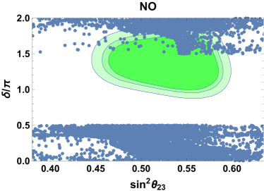
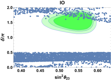
Figure 2: Allowed values for the leptonic mixing parameters for Normal Ordering (NO) and Inverted Ordering (IO). All points lie within the $2\sigma$ regions of the neutrino oscillation parameters. For comparison, the green regions correspond to the generic 90, 95 and 99% C.L. regions from the Global fit in[1].

In the above expressions, the angle $\omega_{12}$ can be eliminated using Eq.(49). Thus, the lepton mixing parameters depend on three angles $\omega_{13}$, $\omega_{23}$, $\psi$ (restricted in our analysis to satisfy Eq.(49) with real values for $\lambda_{1}$, $\lambda_{2}$ and $r$), two additional angles coming from charged lepton mixing and subject to $\eta_{1}\sim\eta_{2}\sim\lambda$ and three discrete variables $k_{1}$, $k_{2}$, $k_{3}$ entering in the Majorana phases.

In Figure (2) we show the allowed values for the leptonic Dirac CP violating phase $\delta$ versus the atmospheric mixing parameter $\sin^{2}\theta_{23}$, for both normal and inverted neutrino mass orderings. These values were generated by randomly varying the model parameters $\omega_{13}$, $\omega_{23}$, $\psi$, $|\eta_{1}|$ and $|\eta_{2}|$ within a range that covers reactor and solar mixing angles inside the $2\sigma$ experimentally allowed range. In particular, we varied $|\eta_{1}|$ and $|\eta_{2}|$ in the range $[0.5\lambda,3\lambda]$. Furthermore, the light active neutrino mass scale was randomly varied in the range $10^{-4}\mathrm{eV}<m_{0}<1\mathrm{eV}$, consistent with $2\sigma$ allowed values for the neutrino mass squared splittings.

To close this section we note that, in contrast to the Left-right symmetric models of Refs. [61, 62], where the $\mu-\tau$ symmetry is broken softly, our departure from $\mu-\tau$ symmetry is induced by the mixing in the charged lepton sector, parameterized by the $\eta_{1}$ and $\eta_{2}$ angles, assumed to be of the same order as the Cabibbo angle $\lambda$.

IV Neutrinoless double beta decay

In this section we present the model predictions for neutrinoless double beta ($0\nu\beta\beta$) decay. The effective Majorana neutrino mass parameter is

$$\left|m_{\beta\beta}\right|=\left|\sum_{i=1}^{3}m^{\nu}_{i}U_{ei}^{2}\right|=\left|m^{\nu}_{1}c^{2}_{12}c^{2}_{13}+m^{\nu}_{2}s^{2}_{12}c^{2}_{13}e^{-2i\phi_{12}}+m^{\nu}_{3}s^{2}_{13}e^{-2i\phi_{13}}\right|,$$ (67)

where $m_{\nu_{i}}$ are the light active neutrino masses and $U_{ei}^{2}$ are the squared lepton mixing matrix elements, respectively.

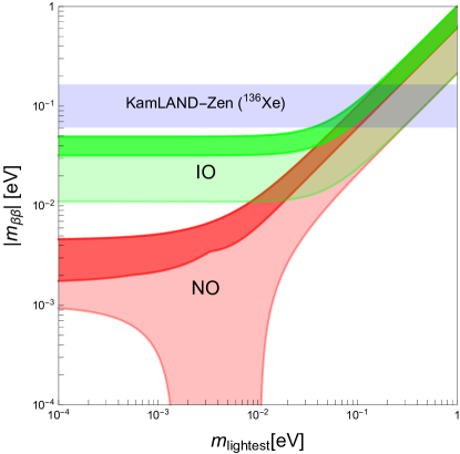
Figure 3: Effective Majorana neutrino mass parameter $|m_{\beta\beta}|$ as a function of the lightest active neutrino mass $m_{\text{lightest}}$ for normal and inverted neutrino mass orderings. The dark regions correspond to points satisfying $2\sigma$ constraints for all mixing parameters. The current sensitivity of the KamLAND-Zen experiment is indicated in purple.

The current experimental sensitivity on the Majorana neutrino mass parameter is illustrated by the horizontal band in Fig. (3) and comes from the KamLAND-Zen limit on the ${}^{136}\mathrm{Xe}$ $0\nu\beta\beta$ decay half-life $T^{0\nu\beta\beta}_{1/2}({}^{136}\mathrm{Xe})\geq 1.07\times 10^{26}$ yr [63], which translates into a corresponding upper bound on $|m_{\beta\beta}|\leq(61-165)$ meV at 90% C.L. as indicated by the horizontal band in Fig. (3). For those of other experiments see Ref. [64, 65, 66, 67, 68]. The “expected” regions for the effective Majorana neutrino mass parameter $|m_{\beta\beta}|$ consistent with the constraints from the current neutrino oscillation data at the $2\sigma$ level are indicated by the other broad shaded bands. There are two cases, corresponding to normal and inverted neutrino mass orderings. These are generic, arising only by imposing current oscillation data. In contrast, the thinner (darker) bands include also the model predictions described in the previous section. These regions are obtained from our generated model points by imposing current neutrino oscillation constraints at the $2\sigma$ level.

One sees that our “predicted” ranges for the effective Majorana neutrino mass parameter have lower bounds in both cases, of normal and inverted mass orderings, indicating that a complete destructive interference amongst the three light neutrinos is always prevented in our model. These lower bounds for the $\mathrm{0}\nu\beta\beta$ amplitude are general predictions of the present model, and can easily be understood.

In fact, as mentioned above, the structure of our $\mu-\tau$ symmetric neutrino mass matrix is a particular case of that in Ref. [54]. Comparing with the results of Ref. [57] one sees that, indeed, the possible destructive interference amongst the three light neutrinos is prevented (as $\lim_{\eta_{1}\rightarrow 0}I_{1,2}=0$), thus explaining the absolute lower bound we obtain.

The experimental sensitivity of $\mathrm{0}\nu\beta\beta$ searches is expected to improve in the near future. For our model, the predicted $\mathrm{0}\nu\beta\beta$ decay rates may be tested by the next-generation bolometric CUORE experiment [69], as well as the next-to-next-generation ton-scale $0\nu\beta\beta$-decay experiments [63, 70, 71, 72].

V Quark masses and mixings

In this section, we illustrate how the model is capable of reproducing the correct masses and mixings in the quark sector. From the quark Yukawa interactions, we find that the up-type mass matrix in the basis $(\overline{u}_{1L},\overline{u}_{2L},\overline{u}_{3L},\overline{T}_{1L},\overline{T}_{2L},\overline{T}_{3L})$ versus $(u_{1R},u_{2R},u_{3R},T_{1R},T_{2R},T_{3R})$ is given by:

$$M_{U}=\left(\begin{array}[]{ccc}0_{2\times 2}&0_{2\times 1}&x\frac{v_{L}}{\sqrt{2}}\\ 0_{1\times 2}&\alpha_{33}\frac{v}{\sqrt{2}}&0_{1\times 2}\\ x^{T}\frac{v_{R}}{\sqrt{2}}&0_{2\times 1}&M_{T}\end{array}\right),\hskip 28.45274ptx=\left(\begin{array}[]{cc}x_{11}\lambda^{2}&x_{12}\lambda\\ 0&x_{22}\end{array}\right),\hskip 28.45274ptM_{T}=\left(\begin{array}[]{cc}m_{T_{1}}&0\\ 0&m_{T_{2}}\end{array}\right),\hskip 28.45274ptm_{t}=\alpha\frac{v}{\sqrt{2}},$$ (68)

while the down type quark mass matrix is given as:

$$M_{D}=\left(\begin{array}[]{cc}0_{3\times 3}&y\frac{v_{L}}{\sqrt{2}}\\ y^{T}\frac{v_{R}}{\sqrt{2}}&M_{B}\end{array}\right),\hskip 28.45274pty=\left(\begin{array}[]{ccc}y_{11}\lambda^{2}&0&y_{13}\lambda^{3}\\ 0&y_{22}\lambda&y_{23}\lambda^{2}\\ 0&0&y_{33}\end{array}\right)\allowbreak,\hskip 28.45274ptM_{B}=\left(\begin{array}[]{ccc}m_{B_{1}}&0&0\\ 0&m_{B_{2}}&0\\ 0&0&m_{B_{3}}\end{array}\right),\allowbreak\allowbreak$$ (69)

expressed in the basis $(\overline{d}_{1L},\overline{d}_{2L},\overline{d}_{3L},\overline{B}_{1L},\overline{B}_{2L},\overline{B}_{3L})$-$(d_{1R},d_{2R},d_{3R},B_{1R},B_{2R},B_{3R})$. Assuming the exotic quark masses to be sufficiently larger than $v_{L}$ and $v_{R}$, it follows that the SM quarks lighter than the top quark all get their masses from a Universal seesaw mechanism mediated by the three exotic up-type and down-type quarks $U_{i}$ and $D_{i}$ ($i=1,2,3$). It is worth mentioning that the top quark does not mix with the remaining up-type quarks. As a result, the SM quark mass matrices take the form:

$$\widetilde{M}_{U} = \left(\begin{array}[]{cc}\frac{v_{L}v_{R}}{2}xM_{T}^{-1}x^{T}&0_{2\times 1}\\ 0_{1\times 2}&m_{t}\end{array}\right)=\left(\begin{array}[]{ccc}\left(x_{12}^{2}+\frac{m_{T_{2}}}{m_{T_{1}}}x_{11}^{2}\lambda^{2}\right)\lambda^{2}\frac{v_{L}v_{R}}{2m_{T_{2}}}&x_{12}x_{22}\lambda\frac{v_{L}v_{R}}{2m_{T_{2}}}&0\\ x_{12}x_{22}\lambda\frac{v_{L}v_{R}}{2m_{T_{2}}}&x_{22}^{2}\frac{v_{L}v_{R}}{2m_{T_{2}}}&0\\ 0&0&m_{t}\end{array}\right)$$ (75)

$$= \left(\begin{array}[]{ccc}\left(\frac{a_{12}^{2}}{a_{22}}+\kappa\lambda^{2}\right)\lambda^{6}&a_{12}\lambda^{5}&0\\ a_{12}\lambda^{5}&a_{22}\lambda^{4}&0\\ 0&0&\alpha\end{array}\right)\allowbreak\allowbreak\frac{v}{\sqrt{2}},$$ (79)

$$\widetilde{M}_{D} = \frac{v_{L}v_{R}}{2}yM_{B}^{-1}y^{T}=\left(\begin{array}[]{ccc}\left(\frac{m_{B_{3}}}{m_{B_{1}}}y_{11}^{2}+y_{13}^{2}\lambda^{2}\right)\lambda^{4}&y_{13}y_{23}\lambda^{5}&y_{13}y_{33}\lambda^{3}\\ y_{13}y_{23}\lambda^{5}&\left(\frac{m_{B_{3}}}{m_{B_{2}}}y_{22}^{2}+y_{23}^{2}\lambda^{2}\right)\lambda^{2}&y_{23}y_{33}\lambda^{2}\\ y_{13}y_{33}\lambda^{3}&y_{23}y_{33}\lambda^{2}&y_{33}^{2}\end{array}\right)\allowbreak\frac{v_{L}v_{R}}{2m_{B_{3}}}$$ (83)

$$= \left(\begin{array}[]{ccc}b_{11}\lambda^{7}&b_{12}\lambda^{8}&b_{13}\lambda^{6}\\ b_{12}\lambda^{8}&b_{22}\lambda^{5}&b_{23}\lambda^{5}\\ b_{13}\lambda^{6}&b_{23}\lambda^{5}&b_{33}\lambda^{3}\end{array}\right)\allowbreak\frac{v}{\sqrt{2}},$$ (87)

where we have set $v_{L}=\lambda^{4}\frac{\sqrt{2}v}{v_{R}}m_{T_{2}}=\lambda^{3}\frac{\sqrt{2}v}{v_{R}}m_{B_{2}}$. Let us note that in our model, the dominant contribution to the Cabbibo mixing arises from the up-type quark sector, whereas the down-type quark sector contributes to the remaining CKM mixing angles. In order to recover the low energy quark flavor data, we assume that all dimensionless parameters of the SM quark mass matrices are real, except for $b_{13}$, taken to be complex.

Starting from the following benchmark point:

$$a_{12} \simeq -1.375,\hskip 28.45274pta_{22}\simeq 1.599,\hskip 28.45274pt\kappa\simeq 1.724,\hskip 28.45274pt\alpha\simeq 0.989,\hskip 28.45274ptb_{11}\simeq 0.595,\hskip 28.45274ptb_{12}\simeq 0.847,$$

$$b_{22} \simeq 0.640,\hskip 28.45274pt\left|b_{13}\right|\simeq 1.168,\hskip 28.45274pt\arg\left(b_{13}\right)\simeq-158.2^{\circ},\hskip 28.45274ptb_{23}\simeq 1.104,\hskip 28.45274ptb_{33}\simeq 1.414$$ (88)

Observable	Model value	Experimental value
$m_{u}(\mathrm{MeV})$	$1.92$	$1.45_{-0.45}^{+0.56}$
$m_{c}(\mathrm{MeV})$	$744$	$635\pm 86$
$m_{t}(\mathrm{GeV})$	$172.1$	$172.1\pm 0.6\pm 0.9$
$m_{d}(\mathrm{MeV})$	$2.82$	$2.9_{-0.4}^{+0.5}$
$m_{s}(\mathrm{MeV})$	$60.3$	$57.7_{-15.7}^{+16.8}$
$m_{b}(\mathrm{GeV})$	$2.82$	$2.82_{-0.04}^{+0.09}$
$\sin\theta_{12}$	$0.225$	$0.22536\pm 0.00061$
$\sin\theta_{23}$	$0.0414$	$0.0414\pm 0.0012$
$\sin\theta_{13}$	$0.00355$	$0.00355\pm 0.00015$
$J$	$3.08\times 10^{-5}$	$2.96_{-0.16}^{+0.20}\times 10^{-5}$

Table 6: Model and experimental values of the quark masses and CKM parameters.

one can check that the resulting values for the physical quark mass spectrum [73, 74], mixing angles and Jarlskog invariant [75] are indeed consistent with the experimental data, as shown in Table 6. This establishes the viability of our model also for the quark sector. Note that the dimensionless parameters of the benchmark point (V) are all $\sim O(1)$ in absolute value. This means that our model reproduces the quark mass and mixing hierarchy by its symmetries resulting in certain distribution of the powers of $\lambda$ among the entries of the mass matrices (79), (87).

VI Features of the model

We now sum up the main theoretical features of our model.

1. Only the top quark and the gauge singlet Majorana neutrinos $\Omega_{i}$ ($i=1,2,3$) acquire masses from renormalizable Yukawa interactions. The exotic charged fermions all have bare tree level mass terms.

2. The masses for the SM charged fermions lighter than the top quark arise from a Universal Seesaw mechanism mediated by charged exotic fermions. The quark mixing angles and the hierarchy between quark masses arise from the spontaneous breaking of the $Z_{6}\otimes Z_{12}$ discrete group.

3. The Cabibbo mixing arises from the up-type quark sector, whereas the down-type quark sector induces the remaining CKM mixing angles. On the other hand, the leptonic mixing parameters receive their dominant contributions from the light active neutrino mass matrix, whereas the charged lepton mass matrix provides Cabibbo-sized corrections to these parameters.

4. The masses for the light active neutrinos emerge from a one loop level inverse seesaw mechanism, whose radiative nature is guaranteed by the spontaneously broken $Z_{4}$ and $Z_{12}$ symmetries, with $Z_{12}$ spontaneously broken down to a preserved $Z_{2}$ symmetry.

5. The mass terms for the gauge singlet sterile neutrinos $S_{i}$ ($i=1,2,3$) are generated from at one loop level, mediated by the real and imaginary components of the electrically neutral gauge singlet scalar $\varphi$ as well as by the gauge singlet Majorana neutrinos $\Omega_{i}$ ($i=1,2,3$). These mass terms break lepton number by two units, triggering the one loop level inverse seesaw mechanism responsible for the light active neutrino masses.

VII Discussion and Conclusions

In summary, we have built a viable extension of the left-right symmetric electroweak extension of the Standard Model capable of explaining the current pattern of SM fermion masses and mixings. Our model is based on the $\Delta(27)$ discrete symmetry, supplemented by the $Z_{4}\otimes Z_{6}\otimes Z_{12}$ discrete family group. In our model, the masses of the light active neutrinos emerge from a one loop level inverse seesaw mechanism, whereas the masses of the Standard Model charged fermions lighter than the top quark are produced by a Universal Seesaw mechanism. Of the Standard Model fermions only the top quark acquires mass through a tree level renormalizable Yukawa interaction. In our model the Cabibbo mixing arises from the up-type quark sector whereas the down-type quark sector contributes to the other CKM mixing angles. On the other hand, the leptonic mixing parameters receive their dominant contributions from the light active neutrino mass matrix, whereas the SM charged lepton mass matrix provide Cabibbo sized corrections. The observed hierarchy of SM charged fermion masses and mixing angles is caused by the spontaneous breaking of the $\Delta\left(27\right)\otimes Z_{6}\otimes Z_{12}$ discrete flavor group, whereas the radiative nature of the inverse seessaw mechanism is guaranteed by spontaneously broken $Z_{4}$ and $Z_{12}$ symmetries, having $Z_{12}$ spontaneously broken down to a preserved $Z_{2}$ symmetry. Our model features a generalized $\mu-\tau$ symmetry and predicts a restricted range of neutrino oscillations parameters, with the neutrinoless double beta decay amplitude lying at the upper ranges associated to normal and inverted neutrino mass ordering.

Notice also that our low-scale left-right symmetric radiative seesaw scheme not only accounts for the light neutrino masses and mixings that lead to oscillations and $0\nu\beta\beta$-decay, but can also lead to signatures that can make it testable at collider experiments such as the LHC. For example, the heavy quasi Dirac neutrinos can be produced in pairs at the LHC, via a Drell-Yan mechanism mediated by a heavy non Standard Model neutral gauge boson $Z^{\prime}$. These heavy quasi Dirac neutrinos can decay into a Standard Model charged lepton and $W$ gauge boson, due to their mixings with the light active neutrinos. Thus, the observation of an excess of events in the dilepton final states with respect to the SM background, would be a signal supporting this model at the LHC. Moreover, lepton flavor violation is expected in these decays, even if suppressed at low energies [76, 77]. A detailed study of the collider phenomenology of this model is beyond the scope of the present paper and is left for future studies.