Mxdrfile: read and write Gromacs trajectories with Matlab

Abstract

Progress in hardware, algorithms, and force fields are pushing the scope of molecular dynamics (MD) simulations towards the length- and time scales of complex biochemical processes. This creates a need for developing advanced analysis methods tailored to the specific questions at hand. We present mxdrfile, a set of fast routines for manipulating the binary xtc and trr trajectory files formats of Gromacs, one of the most commonly used MD codes, with Matlab, a powerful and versatile language for scientific computing. The unique ability to both read and write binary trajectory files makes it possible to leverage the broad capabilities of Matlab to speed up and simplify the development of complex analysis and visualization methods. We illustrate these possibilities by implementing an alignment method for buckled surfaces, and use it to briefly dissect the curvature-dependent composition of a buckled lipid bilayer. The mxdrfile package, including the buckling example, is available as open source at http://kaplajon.github.io/mxdrfile/.

I Introduction

Molecular dynamics (MD) simulations are useful complements to experimental studies of many biomolecular processes, because they generate information about all classical degrees of freedom of the system with atomic resolution by solving Newton’s equations of motion.

The length- and time-scales that are accessible to atomistic MD simulations are increasing rapidly, due to increasing computer power and improved algorithmic performance, which means that it becomes feasible to simulate increasingly complex systems and processes Pronk et al. (2013). Even larger and longer simulations are possible by using coarse-graining, where detailed structural features are systematically removed from the models in order to increase computational speed Reynwar et al. (2007); Marrink et al. (2007). Simulations of complex processes often require customized analysis and visualization methods that are most easily developed using high-level languages for general-purpose scientific computing. This, in turn, requires efficient methods to read and write the simulated MD trajectories in such environments which is not a trivial task, as trajectory files often use non-intuitive formats to minimize file size.

Here, we present the mxdrfile toolbox, which can read and write binary trajectories from one of the most popular and powerful MD codes, Gromacs Pronk et al. (2013), with Matlab, a powerful and widely used language for general-purpose scientific computing. Our routines utilize the loadlibrary functionality in Matlab to access the binary files directly through the Gromacs xdr library, which was developed precisely to allow easy interfacing with external analysis tools xdr . This offers an efficient and robust implementation, and extends the functionality of previous Gromacs parsers for Matlab which are read-only Arthur ; Ribarics ; Dien et al. (2014).

II Basic usage

Reading or writing Gromacs trajectories (xtc or trr files) are done in three steps: opening a binary file for reading or writing, stepping through the trajectory to read or write each frame, and finally closing the file. Using the wrapper commands of mxdrfile, loading and parsing a trajectory requires about 10 lines of code:

 loadmxdrfile; % Load the xdrfile library
 % open files for reading and writing
 [~,rTraj]=inittraj(’test.xtc’,’r’);
 [~,wTraj]=inittraj(’testwrite.xtc’,’w’);
 % read first frame
 [rstatus,traj]=read_xtc(rTraj);
 % parse trajectory
 while(not(rstatus))
    % Do something with the coordinates
    traj.x.value=traj.x.value*0.8;
    % Write newcoords to a new xtc file
    wstatus=write_xtc(wTraj, traj);
    % read next frame
    [rstatus,traj]=read_xtc(rTraj);
 end
% close files
[status,rTraj]=closetraj(rTraj);
[status,wTraj]=closetraj(wTraj);

Figure 1: Component distributions in a coarse-grained buckled POPE/POPG bilayer interacting with a single Magainin peptide Gómez-Llobregat et al. (2016). a) Theoretical buckled surface used for alignment. b) Simulation snapshot. c-f) Mass density plots in the $xz$-plane of vrious components. Molecular graphics generated with VMD Humphrey et al. (1996).

For read-only parsing, an @mxdrfile class provides even more compact access to both trajectory types, as illustrated by the following minimal example:

 loadmxdrfile; % Load the xdrfile library
 % open file and read the first frame
 trj=mxdrfile(’test.xtc’);
 z=[];
 % Loop over the trajectory frames
 while(~trj.status)
     z(end+1)=mean(trj.x.value(3,:));
     trj.read(); % move to next frame
 end
 clear trj % also closes trj file

III Case study: membrane buckling

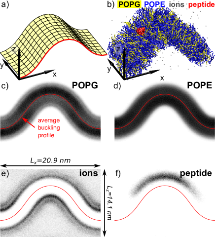
Next, we consider an application that makes use of Matlab’s numerical capabilities, by studying the curvature-dependent composition of a lipid bilayer using simulated buckling. Buckling a lipid bilayer by compressing the projected area of a rectangular patch creates a shape that closely follows the classical Euler buckling profile Noguchi (2011); Hu et al. (2013), and thus presents a range of positive and negative curvatures that makes it an excellent model system for simulating membrane curvature sensing Gómez-Llobregat et al. (2016) (see Fig. 1a,b). The shape is maintained by simulating an ensemble where the projected area is kept fixed (but the box height may be used to maintain constant pressure).

However, to extract useful information, one must remove random drift of the membrane profile from the simulation in order to analyse motions relative to the buckled membrane profile. This presents a challenging alignment problem. Since the lipids move randomly within the membrane plane, simply minimizing the RMSD to some reference configuration will not work well. An alternative approach is to use the theoretical Euler buckling profile (Fig. 1a) as a template, and align by minimizing the total square distance between the buckling profile and the beads at the end of the lipid tails, which are situated near the membrane midplane. The degree of buckling of the template shape should also be flexible to accomodate small area fluctuations of the membrane.

The Euler shape depends on a dimensionless compression factor $\gamma=(L-L_{x})/L$, where $L$ is the arclength along the buckled direction, and $L_{x}$ is the corresponding projected length. Hence, if we parameterize the buckled profile as a function of $\gamma$ for a reference size, the general case can be obtained by shifting and scaling. Following ref. Gómez-Llobregat et al. (2016), we choose $L_{x}=1$ as reference, and write the general buckling profile in the $x,z$ plane as a parametric curve

$$x=L_{x}\big{(}s+\xi(s,\gamma)\big{)},\quad z=L_{x}\zeta(s,\gamma),$$ (1)

where $s$ is an arclength-like parameter that we will take to be normalized to have period 1. If the beads to align have coordinates $\{x_{i},z_{i}\}$, $i=1,2,\ldots$, the alignment problem consists of minimizing the total square distance

$$\sum_{i}\Big{(}x_{0}+L_{x}\big{(}s+\xi(s_{i},\gamma)\big{)}-x_{i}\Big{)}^{2}+\Big{(}z_{0}+L_{x}\big{(}\zeta(s_{i},\gamma)\big{)}-z_{i}\Big{)}^{2}$$ (2)

w.r.t. the shape parameter $\gamma$, the projected positions $s_{i}$, and the overall displacements $x_{0},z_{0}$.

We used mxdrfile to solve this alignment problem in Matlab. An efficient numerical solution of this non-linear least-squares problem requires good minimization routines (which Matlab has) as well as fast evaluation of $\xi,\zeta$ and their partial derivatives w.r.t $s,\gamma$. The Euler buckling problem has a partly implicit analytical solution in terms of elliptic functions Noguchi (2011). We chose a brute-force numerical approach instead, and used Matlab’s built-in boundary value solver to compute buckling profiles for the reference case $L_{x}=1$, from which we expanded $\xi,\zeta$ in truncated Fourier series that for symmetry reasons take the forms

$$\xi(s,\gamma)= \sum_{n=1}^{N}a_{n}^{(x)}(\gamma)\sin(4\pi ns),$$ (3)

$$\zeta(s,\gamma)= a_{0}^{(z)}(\gamma)+\sum_{n=1}^{N}a_{n}^{(z)}(\gamma)\cos(2\pi(2n-1)s).$$ (4)

Only a few terms are needed, and partial derivatives w.r.t. $s$ are now easily constructed. For the coefficients $a_{j}^{(x,z)}(\gamma)$, we used Matlab’s piece-wise polynomial interpolation, which can be exactly differentiated w.r.t. $\gamma$.

We applied the above analysis to a 15 $\mathrm{\SIUnitSymbolMicro s}$ Martini Marrink et al. (2007); de Jong et al. (2013) simulation of the antibacterial amphipathic peptide magainin interacting with a buckled two-component lipid bilayer (70:30 POPE:POPG, see Ref. Gómez-Llobregat et al. (2016) for details). Fig. 1c shows transverse density profiles of the two lipid species, the counter ions, and the peptide, all of which display non-trivial curvature-dependent distributions. An animation showing part of the trajectory before and after alignment is shown in supplementary movie S1.

IV Conclusions

We provide a set of routines to enable read and write access to Gromacs binary xtc and trr trajectory file formats in Matlab. The code was showcased with an application to solve the alignment problems related to Euler buckling of lipid bilayers. We believe that the ability to parse and manipulate Gromacs trajectories will be similarly useful in tackling future complex simulation problems, utilizing the full potentials of Gromacs and Matlab.

The mxdrfile package, including the buckling example, is available as open source at http://kaplajon.github.io/mxdrfile/.

Acknowledgements

Finanical support from the Carl Trygger Foundation (J.K. through Arnold Maliniak), the Wenner-Gren Foundations (M.L.) and the Swedish Foundation for Strategic Research via the Center for Biomembrane Research (M.L.) are gratefully acknowledged.

References

- Pronk et al. (2013) Sander Pronk, Szilárd Páll, Roland Schulz, Per Larsson, Pär Bjelkmar, Rossen Apostolov, Michael R. Shirts, Jeremy C. Smith, Peter M. Kasson, David van der Spoel, Berk Hess, and Erik Lindahl, “GROMACS 4.5: a high-throughput and highly parallel open source molecular simulation toolkit,” Bioinformatics 29, 845–854 (2013).
- Reynwar et al. (2007) Benedict J. Reynwar, Gregoria Illya, Vagelis A. Harmandaris, Martin M. Muller, Kurt Kremer, and Markus Deserno, “Aggregation and vesiculation of membrane proteins by curvature-mediated interactions,” Nature 447, 461–464 (2007).
- Marrink et al. (2007) Siewert J. Marrink, H. Jelger Risselada, Serge Yefimov, D. Peter Tieleman, and Alex H. de Vries, “The MARTINI force field: Coarse grained model for biomolecular simulations,” J. Phys. Chem. B 111, 7812–7824 (2007).
- (4) “Gromacs xtc library,” http://www.gromacs.org/Developer_Zone/Programming_Guide/XTC_Library, accessed 2014-09-24.
- (5) Evan Arthur, “Convert gromacs v 4.5 trajectory files into MatLab matrix - file exchange - MATLAB central,” .
- (6) Reiner Ribarics, “Gromacs matlab exchange,” Bitbucket.org/BioSimVienna/gro-mex.
- Dien et al. (2014) Hung Dien, Charlotte M. Deane, and Bernhard Knapp, “Gro2mat: A package to efficiently read gromacs output in MATLAB,” J. Comput. Chem. 35, 1528–1531 (2014).
- Gómez-Llobregat et al. (2016) Jordi Gómez-Llobregat, Federico Elías-Wolff, and Martin Lindén, “Anisotropic membrane curvature sensing by amphipathic peptides,” Biophys. J. 110, 197–204 (2016).
- Humphrey et al. (1996) William Humphrey, Andrew Dalke, and Klaus Schulten, “VMD: Visual molecular dynamics,” J. Mol. Graphics 14, 33–38 (1996).
- Noguchi (2011) Hiroshi Noguchi, “Anisotropic surface tension of buckled fluid membranes,” Phys. Rev. E 83, 061919 (2011).
- Hu et al. (2013) Mingyang Hu, Patrick Diggins, and Markus Deserno, “Determining the bending modulus of a lipid membrane by simulating buckling,” J. Chem. Phys. 138, 214110–214110–13 (2013).
- de Jong et al. (2013) Djurre H. de Jong, Gurpreet Singh, W. F. Drew Bennett, Clement Arnarez, Tsjerk A. Wassenaar, Lars V. Schäfer, Xavier Periole, D. Peter Tieleman, and Siewert J. Marrink, “Improved parameters for the Martini coarse-grained protein force field,” J. Chem. Theory Comput. 9, 687–697 (2013).