Simulation-based inference methods for partially observed Markov model via the R package is2

Duc Anh Doan, Dao Nguyen, Xin Dang Simulation-based inference methods Simulation-based inference methods Partially observed Markov process (POMP) models are powerful tools for time series modeling and analysis. Inherited the flexible framework of R package pomp, the is2 package extends some useful Monte Carlo statistical methodologies to improve on convergence rates. A variety of efficient statistical methods for POMP models have been developed including fixed lag smoothing, second-order iterated smoothing, momentum iterated filtering, average iterated filtering, accelerate iterated filtering and particle iterated filtering. In this paper, we show the utility of these methodologies based on two toy problems. We also demonstrate the potential of some methods in a more complex model, employing a nonlinear epidemiological model with a discrete population, seasonality, and extra-demographic stochasticity. We discuss the extension beyond POMP models and the development of additional methods within the framework provided by is2. Markov processes, state space model, stochastic dynamical system, maximum likelihood, fixed lag smoothing, R Markov processes, state space model, stochastic dynamical system, maximum likelihood, fixed lag smoothing, R Duc Anh Doan
Department of Mathematics
University of Mississippi
38677 Mississippi, USA
E-mail:
Dao Nguyen
Department of Mathematics
University of Mississippi
38677 Mississippi, USA
E-mail:
URL: https://math.olemiss.edu/dao-nguyen/
Xin Dang
Department of Mathematics
University of Mississippi
38677 Mississippi, USA
E-mail:
URL: home.olemiss.edu/~xdang/

1 Introduction

In data analysis, partially observed Markov process (POMP) models (also known as state space models) have been known of as powerful tools in modeling and analyzing time series in many disciplines such as ecology, econometric, engineering and statistics. However, making inferences on POMP models can be problematic because of the presence of incomplete measurements, and possibly weakly identifiable parameters. Typical methods for inference (e.g., maximum likelihood) with strong assumptions of linear Gaussian models have often resulted in undesired outcomes, especially when the assumptions are violated. Simulation-based inferences, also called plug-and-play inferences, are characterized as the dynamic model entering the statistical computations through a numerical solution of the sample paths (Bretó et al., 2009). As a result, there has been a lot of interest in simulation-based inference for POMP models, largely software development for this class of inference. The pomp software package (King et al., 2014) was developed to provide a general representation of a POMP model where several algorithms implemented within pomp are applicable to arbitrary POMP models (Ionides et al., 2006; Toni et al., 2009; Andrieu et al., 2010; Wood, 2010; Ionides et al., 2015; Nguyen and Ionides, 2017). However, since pomp is designed years ago for conventional POMP models, applicabilities of these inference methods for very large-scale data set remains an open question. In particular, in the big data regime when the convergence rate is critical, some recently efficient methods have not yet been parts of pomp. Motivated by this need and the popularity of pomp, we develop is2 software package to provide additional efficient algorithms. Based on the recent developments of stochastic optimization literature, we focus more on inference methods using advanced machine learning algorithms, which we consider as a complement of pomp rather than a competing software package.

Specifically, we extend the core functionality of pomp to include particle fixed lag smoothing which is more stable than filtering and reduces computational expense of traditional smoothing. In addition, we provide several efficient inference methods using the full information and full likelihood of the data. The first algorithm developed to carry out such inference is the second order iterated smoothing algorithm of Nguyen and Ionides (2017). Doucet et al. (2013) showed that sequential Monte Carlo smoothing can give the first derivative as well as Hessian estimation of the log likelihood that have better asymptotic convergence rates than those used for iterated filtering in pomp. One can apply these moments approximations of Doucet et al. (2013) in a Newton-Raphson type optimization algorithm. We develop a modification of the theory of Doucet et al. (2013) giving rise to a new algorithm, which empirically shows enhanced performance over other available methods on standard benchmarks. The second implemented algorithm is called momentum iterated filtering where we accumulate a velocity vector in the persistent increase directions of the log likelihood function across iterations. This will help the algorithm achieve results of the same level of accuracy in fewer iterations. The third algorithm developed for simulation-based inference is accelerate iterated filtering. Unlike original iterated filtering, the accelerate method exploits an approximation of the gradient of log likelihood in the accelerated scheme where the convexity and unbiasedness restrictions are relaxed. The theoretical underlying is described in more details in (Nguyen, 2018). By avoiding the computational expenses of Hessian, this method is very promising as it is a first order but obtains the quadratic convergence rate of the second order approaches. The fourth algorithm included in the package is average iterated filtering, which has typically been motivated by two time scales optimization process. In this algorithm, the slower scale will be sped up by the faster scale, resulting in a very attractive approach with a simple computation but a fast convergence rate. Lastly, we implement a particle version of iterated filtering algorithm where gradient of the log likelihood as the by-product of iterated filtering is used to improve the proposal distribution in Langevin algorithm in the context of simulation-based algorithm. This algorithm enables a routine full-information plug-and-play Bayesian inference for POMP models, inheriting several advantages such as shortening the burn-in, accelerating the mixing of the Markov chain at the stationary period, and simplifying tuning (Dahlin et al., 2015a).

The key contributions of this paper are three-fold. First, we provide users with ample of new efficient algorithms for simulation-based inferences, demonstrating its ease of use in practical problems. Second, advanced machine learning simulation-based inference algorithms are not only attractive in theory, but we show them also have good numerical performance in practice. In particular, they are applied in both simple toy problems and a challenging scientific problem and they give impressive results. Third, we provide a general framework for interested users not only they can use but also they can develop new algorithms based on smoothing instead of filtering. Consequently, as moments are by-products of iterated smoothing, advanced methods such as proximal optimization simulation-based inference could be implemented in our framework.

The paper is organized as follows. In Section 2, we introduce some backgrounds of simulation-based inferences we investigate. In Section 3, we describe the fixed lag smoothing algorithm in the context of partially observed Markov models, which are later extended to different plug-and-play methodologies. We also give a brief description on advantages and disadvantages of each methodology. Section 4 presents two toy problems, showing substantial gains for our new methods over current alternatives, while Section 5 illustrates the potential applications of some efficient methods in a challenging inference problem of fitting a malaria transmission model to time series data. We conclude in Section 6 with the suggesting of the future works to be extended. More experiments and different functionalities can also be found in the package repository.

2 Background of models and simulation-based inferences

Let $\{X(t),\ t\in\mathbb{T}\}$ be a Markov process with $X(t)$ taking values in a measurable space $\mathcal{X}$ with a finite subset $t_{1}<t_{2}<\cdots<t_{N}$ at which $X(t)$ is observed, together with some initial time $t_{0}<t_{1}$. We write $X_{0:N}=(X_{0},\ \ldots,\ X_{N})=(X(t_{0}),\ \ldots,\ X(t_{N}))$ and hereafter for any generic sequence $\{X_{n}\}$, we shall use $X_{i:j}$ to denote $(X_{i},\ X_{i+1},\ \ldots,\ X_{j})$. The distribution of $X_{0:N}$ is characterized by the initial density $X_{0}\sim\mu(x_{0};\theta)$ and the conditional density of $X_{n}$ given $X_{n-1}$, written as $f_{n}(x_{n}|x_{n-1};\theta)$ for $1\leq n\leq N$ where $\theta$ is an unknown parameter in $\mathbb{R}^{d}$. The process $\{X_{n}\}$ takes values in a measurable space $\mathcal{Y}$, being only observed through another process $\{Y_{n},n=1,\dots,N\}$ . The observations are assumed to be conditionally independent given $\{X_{n}\}$. Their probability density is of the form

$$p_{Y_{n}|Y_{1:n-1},\ X_{0:n}}(y_{n}|y_{1:n-1},\ x_{0:n};\theta)=g_{n}(y_{n}|x_{n};\theta),$$

for $1\leq n\leq N$. It is assumed that $X_{0:N},\mathrm{Y}_{1:N}$ have a joint density $p_{X_{0:N},Y_{1:N}}(x_{0:N},y_{1:N};\theta)$ on $\mathcal{X}^{N+1}\times\mathcal{Y}^{N}$. The data are a sequence of observations $y_{1:N}^{*}=(y_{1}^{*},\ \ldots,\ y_{N}^{*})\in\mathcal{Y}^{N}$, considered as fixed and we write the $\log$ likelihood function of the data for the POMP model as

$$\ell(\theta) = \log p_{Y_{1:N}}(y_{1:N}^{*};\theta)$$

$$= \log\int\mu(x_{0};\theta)\prod_{n=1}^{N}f_{n}(x_{n}|x_{n-1};\theta)\ g_{n}(y_{n}^{*}|x_{n};\theta)\ dx_{0:N}.$$

A practical limitation for those models is that it is difficult or even impossible to compute the log-likelihood and hence to compute the MLE in closed form. Therefore, MLE process often uses first order stochastic approximation (Kushner and Clark, 2012), which involves a Monte Carlo approximation to a difference equation,

$$\theta_{m}=\theta_{m-1}+\gamma_{m}\nabla\ell(\theta_{m-1}),$$

where $\theta_{0}\in\Theta$ is an arbitrary initial estimate and $\{\gamma_{m}\}_{m\geq 1}$ is a sequence of step sizes with ${\sum_{m\geq 1}\gamma_{m}=\infty}$ and ${\sum_{m\geq 1}\gamma_{m}^{2}<\infty}$. The algorithm converges to a local maximum of $\ell(\theta)$ under regularity conditions. The term $\nabla\ell(\theta)$, also called the score function, is shorthand for the $\mathbb{R}^{d}$-valued vector of partial derivatives,

$$\nabla\ell(\theta)=\frac{\partial\ell(\theta)}{\partial\theta}.$$

Sequential Monte Carlo (SMC) approaches have previously been developed to estimate the score function (Poyiadjis et al., 2009; Nemeth et al., 2016b; Dahlin et al., 2015b). However under plug-and-play setting, which does not requires the ability to evaluate transition densities and their derivatives, these approaches are not applicable. Consider a parametric model consisting of a density $p_{Y}(y;\theta)$ with the log-likelihood of the data $y^{*}\in\mathcal{Y}$ given by $\ell(\theta)=\log p_{Y}(y^{*};\theta)$. A stochastically perturbed model corresponding to a pair of random variables $(\breve{\Theta},\breve{Y})$ having a joint probability density on $\mathbb{R}^{d}\times\mathcal{Y}$ can be defined as

$$p_{\breve{\Theta},\breve{Y}}(\breve{\vartheta},\ y;\theta,\ \tau)=\tau^{-d}\kappa\left\{\tau^{-1}(\breve{\vartheta}-\theta)\right\}p_{Y}(y;\breve{\vartheta}).$$

Suppose some regularity conditions, (Doucet et al., 2013) showed that

$$\left|\tau^{-2}\Sigma^{-1}\breve{\mathbb{E}}\left(\breve{\Theta}-\theta\left|\breve{Y}=y^{*}\right.\right)-\nabla\ell\left(\theta\right)\right|<C\tau^{2}.$$ (1)

These approximations are useful for latent variable models, where the log likelihood of the model consists of marginalizing over a latent variable, $X$,

$$\ell(\theta)=\log\int{p_{{X},{Y}}(x,y^{*};\theta)\,dx}.$$

In latent variable models, the expectation in equation (1) can be approximated by Monte Carlo importance sampling, as proposed by Ionides et al. (2011) and Doucet et al. (2013). In Nguyen and Ionides (2017), the POMP model is a specific latent variable model with ${X}=X_{0:N}$ and ${Y}=Y_{1:N}$. A perturbed POMP model is defined to have a similar construction to a perturbed latent variable model with ${\breve{X}}=\breve{X}_{0:N}$, $\breve{Y}=\breve{Y}_{1:N}$ and $\breve{\Theta}=\breve{\Theta}_{0:N}$. Ionides et al. (2011) perturbed the parameters by setting $\breve{\Theta}_{0:N}$ to be a random walk starting at $\theta$, whereas Doucet et al. (2013) took $\breve{\Theta}_{0:N}$ to be independent additive white noise perturbations of $\theta$. Taking advantage of the asymptotic developments of Doucet et al. (2013) while maintaining some practical advantages of random walk perturbations for finite computations, Nguyen and Ionides (2017) show that $\nabla{\ell}\left(\theta\right)$ of the extended model can be approximated as follows.

Theorem 1

(Theorem 2 of Nguyen and Ionides (2017)) Suppose assumptions 1, 2 and 5 of (Nguyen and Ionides, 2017), there exists a constant $C$ independent of $\tau,\tau_{1},...\tau_{N}$ such that,

$$\left|\nabla\ell\left(\theta\right)-\tau^{-2}\Psi^{-1}\left\{\tau_{0}^{-2}\breve{\mathbb{E}}\left(\breve{\Theta}_{0}-\theta|\breve{Y}_{1:N}=y_{1:N}^{*}\right)\right\}\right|<C\tau^{2},$$

where $\Psi$ is the non-singular covariance matrix associated to $\psi$.

Nguyen and Ionides (2017) also presented an alternative variation on these results which leads to a more stable Monte Carlo estimation.

Theorem 2

(Theorem 3 of Nguyen and Ionides (2017)) Suppose assumptions 1,2, 5 as in Nguyen and Ionides (2017). In addition, assume that $\tau_{n}=O(\tau^{2})$ for all $n=1\ldots N$, the following hold true,

$$\left|\nabla\ell\left(\theta\right)-\frac{1}{N+1}\tau^{-2}\tau_{0}^{-2}\Psi^{-1}\sum_{n=0}^{N}\left\{\breve{\mathbb{E}}\left(\breve{\Theta}_{n}-\theta|\breve{Y}_{1:N}=y_{1:N}^{*}\right)\right\}\right|=O(\tau^{2}).$$ (2)

These theorems are useful for our investigated simulation-based inference approaches because we can approximate the gradient of the likelihood of the extended model to the second order of $\tau$ using either particle filtering or particle smoothing, which fits well with our inference framework in the next section.

3 Methodology for POMP models

We are mostly interested in full-information, either Bayesian or frequentist and plug-and-play methods. Table 3 provides a list of several inference methodologies for POMP models implemented in is2.

Implemented algorithms
	Frequentist	Bayesian
Full information	Second-order iterated smoothing (is2, section 3.2)	Particle iterated filtering (pmif, section 3.6)
	Momentum iterated filtering (Momentum-Mif, section 3.3)
	Accelerate iterated filtering (aif, section 3.4),
	Average iterated filtering (avif, section 3.5)

Table 1: Plug-and-play inference methods for POMP models, implemented in is2.

3.1 The likelihood function and particle smoothing

The structure of a POMP model indicates its log likelihood $\ell(\theta)$ can be expressed as the sum of conditional log likelihoods. Typically $\ell(\theta)$ has no closed form and is generally approximated by Monte Carlo methods. In the primitive bootstrap particle filter, the filtering distribution $p(\mathrm{X}_{t}|\mathrm{y}_{1:t})$ at each time step $t$ is represented by $J$ weighted samples $(x_{t}^{j},\ w_{t}^{j})_{j=1}^{J}$, where $(x_{t}^{j})_{j=1}^{J}$ are random samples of the distribution and the weight $w_{t}^{j}$ is the density at this sample. Initially, each weight is set to $\frac{1}{J}$ and $x_{0}^{j}$ are sampled from the prior distribution $\mu_{0}(dx_{0})$. At each time step $t\geq 1$, we draw a sample $X_{t}^{j}$ from $f_{X_{t}|X_{t-1}}(x_{t}|x_{t-1};\theta)$ and use observation $y_{t}$ to compute $w_{t}^{j}$ such that $w_{t}^{j}\propto g(y_{t}|x_{t}^{j})$ and then we normalize them to sum to 1. Now we sample $\left\{X_{t}^{j}\right\}$ by resampling them with probabilities proportional $\left\{w_{t}^{j}\right\}$. The process goes on and the log likelihood approximation is estimated by $\ell(\theta)=\sum_{t=1}^{T}\log\big{(}J^{-1}\,\sum_{j=1}^{J}\!w_{t}^{j})$. It has been shown that as $J\rightarrow\infty$, the approximation will approach the true log likelihood (e.g. (Del Moral, 2004)) and $J$ is typically chosen as a fixed large number.

Primitive bootstrap particle filter is often deteriorated quickly, especially when there are outliers in the observations. This leads to the particle depletion problem when the distribution are represented by only a few survival particles. For this reason, particle smoothing is often preferable to particle filtering since the variance of the smoothing distribution is always smaller than that of the filtering distribution. However, a naive particle smoothing algorithm does not get rid of the particle depletion problem entirely and is known for rather computationally expensive (Kitagawa, 1996; Doucet et al., 2000). Many variations of the particle smoothing algorithm have been proposed to ameliorate this problem. Some approaches may improve numerical performance in appropriate situations (Cappé et al., 2007) but typically lose the plug-and-play property, except for fixed lag smoothing. Since we are interested in plug-and-play property, which assists in investigating of alternative models, we will focus here on fixed lag smoothing. Specifically, rather than targeting the sequence of filtering densities, we target the sequence of distribution $p(dx_{t}|y_{1:T})$. It is often reasonable to assume that for sufficiently large $L$, the future state after the $L$ time steps has little information about the current state. This motivates an approximation, in which we only use all observations up to a time $s+L$ for some sufficiently large $L$ when estimating the state at time $s$. Mathematically, this is equivalent to approximating marginally $p(dx_{t}|y_{1:T})$ by $p(dx_{t}|y_{1:t+L})$ for some lag value $L$, and then approximating $p(dx_{t}|y_{1:t+L})$ with the sequence of densities $p(x_{t}|y_{1:t+L})$ for $t=1,2,\ \ldots T-L$ and $p(x_{t}|y_{1:T})$ for $t=T-L+1,\ \ldots T$ (see e.g. (Polson et al., 2008). This is done by representing $p(x_{t}|y_{1:t+L})$ with a set of weighted particles $\{x_{t}^{j},\ w_{t}^{j}\}_{j=1}^{J}$, each of which is a state $x_{t}$.

input: Simulator for $f_{X_{n}|X_{n-1}}(x_{n}{\,|\,}x_{n-1}{\hskip 1.42262pt;\hskip 1.42262pt}\theta)$; evaluator for $f_{Y_{n}|X_{n}}(y_{n}{\,|\,}x_{n}{\hskip 1.42262pt;\hskip 1.42262pt}\theta)$; simulator for $f_{X_{0}}(x_{0}{\hskip 1.42262pt;\hskip 1.42262pt}\theta)$; parameter, $\theta$; data, $y^{*}_{1:N}$; number of particles, $J$.

1 Initialize smoothing particles: simulate ${X}_{0,j}^{F}\sim{f}_{{X}_{0}}\left({\,\cdot\,}{\hskip 1.42262pt;\hskip 1.42262pt}{\theta}\right)$ for $j$ in ${1}\!:\!{J}$.

2 for $n$ in ${1}\!:\!{N}$ do

3      Simulate for prediction: ${X}_{n,j}^{P}\sim{f}_{{X}_{n}|{X}_{n-1}}\big{(}{\,\cdot\,}|{X}_{n-1,j}^{F};{\theta}\big{)}$ for $j\ \text{in}\ {1}\!:\!{J}$.

4      Evaluate weights: $w(n,j)={f}_{{Y}_{n}|{X}_{n}}(y_{n}^{*}|{X}_{n,j}^{P}{\hskip 1.42262pt;\hskip 1.42262pt}{\theta})$ for $j$ in ${1}\!:\!{J}$.

5      Normalize weights: $\tilde{w}(n,j)=w(n,j)/\sum_{m=1}^{J}w(n,m)$.

6      Apply resampling to select indices $k_{1:J}$ with $\mathbb{P}\left[{k_{j}=m}\right]=\tilde{w}(n,m)$.

7      resample: set ${X}_{n,j}^{F}={X}_{n,k_{j}}^{P}$ for $j$ in ${1}\!:\!{J}$.

8      for $n$ in $1:N-L$, let $a_{1}(n,k_{j})=j$, $a{}_{l+1}(n,j)=a_{1}(n-l,a_{l}(n,j))$ for $j$ in $1:J$, $l$ in $1:L-1$

9      Compute conditional log likelihood: $\hat{\ell}_{n|1:n-1}=\log\big{(}J^{-1}\,\sum_{m=1}^{J}\!w(n+L,m)\big{)}$ for $n$ in $1:N-L$ and $\hat{\ell}_{n|1:n-1}=\log\big{(}J^{-1}\,\sum_{m=1}^{J}\!w(N,m)\big{)}$ for $n$ in $N-L+1:N$

10     

11      end

      output: Log likelihood estimate, $\hat{\ell}(\theta)=\sum_{n=1}^{N}\hat{\ell}_{n|1:n-1}$; smoothing sample, $X^{F}_{n+L,1:J}$, for $n$ in ${1}\!:\!{N-L}$ and $X^{F}_{N,1:J}$, for $n$ in ${N-L+1}\!:\!{N}$.

      complexity: $\mathcal{O}\!\left({J}\right)$

Algorithm 1 Fixed lag particle smoothing: psmooth( P, Np = $J$), where P is a class ‘pomp’ object with definitions for rprocess, dmeasure, init.state, coef, and obs.

In the fixed lag smoothing, $x_{t}^{j}$ is obtained by tracing back the lineage of the particle $x_{t+L}^{j}$. Define $a_{1}(x_{s},k_{j})=j$, $a{}_{l+1}(x_{s},j)=a_{1}(x_{s-l},a_{l}(x_{s},j))$ for all $t\leq s<t+L$, then $x_{t}^{j}$ is $x_{t+L}^{a_{L}(x_{t+L},j)}$.

The algorithm of (Kitagawa, 1996) can be used to approximate $p(x_{t}|y_{1:t+L})$ for a suitable value $L$. Choosing an optimal $L$ might be difficult but in general for any given lag, smoothing is often a better choice compared to filtering. Another advantage of a fixed lag smoothing is that the computational complexity is the same as that of the particle filter. We present the fixed lag smoothing algorithm in Algorithm 1.

3.2 Second-order iterated smoothing

Iterated smoothing, a variant of iterated filtering algorithm, enables inference using simulation-based sequential Monte Carlo smoothing. The basic form of iterated smoothing, proposed by Doucet et al. (2013), was found to have favorable theoretical properties such as being more stable than iterated filtering and producing tighter moment approximations. The innovations of Doucet et al. (2013) are perturbing parameters by white noise and basing on a sequential Monte Carlo solution to the smoothing problem. However, it is an open problem whether the original iterated smoothing approach is competitive in practice. Nguyen and Ionides (2017) modified the theory developed by Doucet et al. (2013) in two key regards.

First, random walk parameter perturbations can be used in place of the white noise perturbations of the original iterated smoothing while preserving much of the theoretical support provided by Doucet et al. (2013). Perturbation in this way has some positive effects:

1. It inherits second-order convergence properties by using an approximation of the observed information matrix.

2. It combats computational expense by canceling out some computationally demanding covariance terms.

3. Plug-and-play property, inherited from the sequential Monte Carlo smoothing, is preserved.

Second, Nguyen and Ionides (2017) modified to construct an algorithm which carries out smoothing, in particular fixed lag smoothing. This Taylor-series approach remains competitive with other state of the art inference approaches both in theory and in practice.

By default, iterated smoothing carries out the fixed lag smoothing with a specified number of lag $l$ and an option for choosing either random walk noise or white noise perturbation. A basic version of a second-order iterated smoothing algorithm using random walk noise is available via the method="is2". The second order iterated smoothing algorithm is2 of Nguyen and Ionides (2017) has shown promises in advancing development of simulation-based inferences. In all iterated smoothing methods, by analogy with simulated annealing, it has shown that in the limit as the perturbation intensity approaches zero, the algorithm will reach the maximum likelihood solution. This perturbation process is gradually reduced according to a prescribed cooling schedule in order to allow the likelihood function to converge.

For some time series models, a few unknown initial conditions, called initial value parameters (IVP), are estimated as parameters. As the length of the time series increases, the estimates are not accurate since only early time points have information of the initial state (King et al., 2015). Therefore for these parameters, we only perturb them at time zero. In general, the perturbation distribution is supplied by the user either with each component, $[\theta]_{i}$, of the parameter vector being perturbed independently or simultaneously. By default, the perturbations on the parameters in Algorithms 5 and 5 of Algorithm 2 is a normal distribution and is perturbed independently. In addition, it is always possible to transform the parameters and choose the perturbation distribution of interest to simplify the algorithm.

input: Starting parameter, $\theta_{0}$; simulator for $f_{X_{0}}(x_{0}{\hskip 1.42262pt;\hskip 1.42262pt}\theta)$; simulator for $f_{X_{n}|X_{n-1}}(x_{n}{\,|\,}x_{n-1}{\hskip 1.42262pt;\hskip 1.42262pt}\theta)$; evaluator for $f_{Y_{n}|X_{n}}(y_{n}{\,|\,}x_{n}{\hskip 1.42262pt;\hskip 1.42262pt}\theta)$; data, $y^{*}_{1:N}$; labels, $I\subset\{1,\dots,p\}$, designating IVPs; fixed lag, $L$, for estimating IVPs; number of particles, $J$, number of iterations, $M$; cooling rate, $0<a<1$; perturbation scales, $\sigma_{1:p}$; initial scale multiplier, $C>0$.

1 for $m$ in ${1}\!:\!{M}$ do

2      $\big{[}\Theta_{0,j}^{F}\big{]}_{i}\sim\mathcal{N}\big{(}\big{[}\theta_{m-1}\big{]}_{i},(c^{m-1}\sigma_{i})^{2}\big{)}$ for $j$ in $1:J$, $i$ in $1:d$

3      initialize states: simulate $X_{0,j}^{F}\sim\mu\big{(}{x}_{0};{\Theta_{0,j}^{F}}\big{)}$ for $j$ in $1:J$

4      for $n$ in $1{\;:\;}N$ do

5           Filtering: $\big{[}\Theta_{n,j}^{P}\big{]}_{i}\sim\mathcal{N}\big{(}\big{[}\Theta^{F}_{n-1,j}\big{]}_{i},(c^{m-1}\sigma_{i})^{2}\big{)}$ for $i\notin I$, $j$ in $1:J$

6           Simulate particles: ${X}_{n,j}^{P}\sim{f}_{n}\big{(}{x}_{n}|{X}_{n-1,j}^{F};{\Theta_{n,j}^{P}}\big{)}$ for $j$ in $1:J$

7           Evaluate weights: $w(n,j)=g_{n}(y_{n}^{*}|X_{n,j}^{P};\Theta_{n,j}^{P})$ for $j$ in $1:J$

8           Normalize weights: $\breve{w}(n,j)=w(n,j)/\sum_{u=1}^{J}w(n,u)$

9           Apply resampling to select indices $k_{1:J}$ with $P\left\{k_{u}=j\right\}=\breve{w}\left(n,j\right)$

10           resample particles: $X_{n,j}^{F}=X_{n,k_{j}}^{P}$ and $\Theta_{n,j}^{F}=\Theta_{n,k_{j}}^{P}$ for $j$ in $1:J$

11           fixed-lag smoothing: for $n$ in $1:N-L$, let $a_{1}(n,k_{j})=j$, $a{}_{l+1}(n,j)=a_{1}(n-l,a_{l}(n,j))$ for $j$ in $1:J$, $l$ in $1:L-1$

12           smoothed mean: $\bar{\theta}_{n-L}^{L}=\sum_{j=1}^{J}\breve{w}(n,j)\Theta_{n-L,a_{L}(n,j)}^{P}$ if $n>L$

13           variance:${V}_{n-L,n-L}^{m}=\sum_{j}\breve{w}(n,j)\big{(}\Theta_{n-L,a_{L}(n,j)}^{P}-\bar{\theta}_{n-L}^{L}\big{)}\big{(}\Theta_{n-L,a_{L}(n,j)}^{P}-\bar{\theta}_{n-L}^{L}\big{)}^{\top}$ if $n>L$

14          

15           end

16           for $n$ in $N-L+1:N$ mean: $\bar{\theta}_{N+l-L}^{L}=\sum_{j=1}^{J}\breve{w}(N,j)\Theta_{N+l-L,a_{L-l}(N,j)}^{P}$ for $l$ in $1:L$

17           $[\theta_{m}]_{i}=[\theta_{m-1}]_{i}+V_{1}^{i}\sum_{n=1}^{N}\left(V_{n}^{i}\right)^{-1}\left(\bar{\theta}_{n}^{i}-\bar{\theta}_{n-1}^{i}\right)$ for $i\not\in I$.

18           ${V}_{N+l-L,N+l-L}^{m}=\sum_{j}\breve{w}(N,j)\big{(}\Theta_{N+l-L,a_{L-l}(N,j)}^{P}-\bar{\theta}_{N+l-L}^{L}\big{)}$
                     $\big{(}\Theta_{N+l-L,a_{L-l}(N,j)}^{P}-\bar{\theta}_{N+l-L}^{L}\big{)}^{\top}$ for $l$ in $1:L$

19           update: $S_{m}=c^{-2(m-1)}\Psi^{-1}\sum_{n=1}^{N}\big{[}\left(\bar{\theta}_{n}^{L}-\theta_{m-1}\right)\big{]}$

20           $I_{m}=-c^{-4(m-1)}\Psi^{-1}\left[\sum_{n=1}^{N}\left(V_{n,n}^{m}/(N+1)-c^{2(m-1)}\Psi\right)\right]\Psi^{-1}$

21           update parameters: $\theta_{m}=\theta_{m-1}+I_{m}^{-1}S_{m}$

22           update IVP parameters: $\big{[}\theta_{m}\big{]}_{i}=\frac{1}{J}\sum_{j=1}^{J}\big{[}\Theta^{F}_{L,j}\big{]}_{i}$ for $i\in I$

23          

24           end

           output: Monte Carlo maximum likelihood estimate, $\theta_{M}$.

           complexity: $\mathcal{O}\!\left({JM}\right)$

Algorithm 2 Second-order iterated smoothing: is2(P, start = $\theta_{0}$, Nis = $M$, Np = $J$, rw.sd = $\sigma_{1:p}$, lag = $L$, var.factor = $C$, cooling.factor = $a$), where P is a class ‘pomp’ object with defined rprocess, dmeasure, init.state, and obs components.

This algorithm is especially useful for parameter estimation in state-space models, in which the focus is on continuous space, discrete time and the latent process can be simulated and the conditional density of the observation given the state can be evaluated point-wise up to a multiplicative constant. The parameters are often added to the state space and this modified state-space model has been inferred using sequential Monte Carlo filtering/smoothing. In the literature, there has been a number of previous proposed approaches to estimate the parameter such as (Kitagawa, 1998; Liu and West, 2001; Wan and Van Der Merwe, 2000) but second-order iterated smoothing is distinguished by having an optimal theoretical convergence rate to the maximum likelihood estimate and is fully supported in practice as well.

3.3 Momentum iterated filtering

The underlying theoretical foundation of original iterated filtering (Ionides et al., 2006) is stochastic gradient descent (SGD). It is generally well known that SGD would easily get stuck in ravines where the curvature surfaces are steeper in some dimensions than the others. It would oscillate across the slopes of the ravine and slowly progress to the local optimum, thus slow down the convergence rate. Some motivations to apply momentum method to iterated filtering rather than using the original iterated filtering consist of:

• To accelerate the convergence rate, it accumulates a velocity vector in directions of persistent increase in the log likelihood function across iterations (Sutskever et al., 2013). Specifically, if the dimensions of the momentum term and the gradient are in the same directions, movement in these directions will be accelerated. On the other hand, if the dimensions of the momentum term and the gradient are in the opposite directions, the momentum term will lend a helping hand to dampen the oscillation in these directions. It can be shown that momentum approach requires fewer iterations to get to the identical degree of precision than gradient descent approach (Polyak, 1964).

• Instead of re-weighting the update throughout each eigen-direction proportional to the inverse of the associated curvature, momentum method adapts the learning rate by accumulating changes along the updated path. For high dimensional data, it is notoriously admitted that explicit computation of curvature matrix is expensive or even infeasible. Accumulating this information along the way appears to possess a certain computational advantage, especially for sparse data regime.

• Another crucial merit of momentum method is the capability to avoid getting trapped in its numerous suboptimal local maxima or saddle points. (Dauphin et al., 2014) postulated that the difficulty arises indeed not from local maxima but from saddle points, i.e. points where one dimension slants up and another inclines down. These saddle points are usually surrounded by a plateau of the same error, which makes it notoriously difficult for SGD to get away from, as the gradient is near zero in all dimensions. It is vital to examine to what degree, momentum method escapes such saddle points, particularly, in the high-dimensional setting in which the directions of avoiding points may be few.

input: Starting parameter, $\theta_{0}$; simulator for $f_{X_{0}}(x_{0}{\hskip 1.42262pt;\hskip 1.42262pt}\theta)$; simulator for $f_{X_{n}|X_{n-1}}(x_{n}{\,|\,}x_{n-1}{\hskip 1.42262pt;\hskip 1.42262pt}\theta)$; evaluator for $f_{Y_{n}|X_{n}}(y_{n}{\,|\,}x_{n}{\hskip 1.42262pt;\hskip 1.42262pt}\theta)$; data, $y^{*}_{1:N}$; labels, $I\subset\{1,\dots,p\}$, designating IVPs; fixed lag, $L$, for estimating IVPs; number of particles, $J$, number of iterations, $M$; cooling rate, $0<a<1$; perturbation scales, $\sigma_{1:p}$; initial scale multiplier, $C>0$; momentum term $\gamma$.

1 for $m$ in ${1}\!:\!{M}$ do

2      Initialize parameters: $[\Theta^{F}_{0,j}]_{i}\sim{\mathrm{Normal}}\left([\theta_{0}]_{i},(Ca^{m-1}\sigma_{i})^{2}\right)$ for $i$ in ${1}\!:\!{p}$, $j$ in $1{\;:\;}J$.

3      Initialize states: simulate $X_{0,j}^{F}\sim f_{X_{0}}\big{(}{\,\cdot\,};{\Theta^{F}_{0,j}}\big{)}$ for $j$ in ${1}\!:\!{J}$.

4      Initialize filter mean for parameters: $\bar{\theta}_{0}=\theta_{0}$.

5      for $n$ in $1{\;:\;}N$ do

6           Perturb parameters: $\big{[}\Theta^{P}_{n,j}\big{]}_{i}\sim{\mathrm{Normal}}\left(\big{[}\Theta^{F}_{n-1,j}\big{]}_{i},(a^{m-1}\sigma_{i})^{2}\right)$ for $i\not\in I$, $j$ in $1{\;:\;}J$.

7           Simulate prediction particles: ${X}_{n,j}^{P}\sim{f}_{{X}_{n}|{X}_{n-1}}\big{(}{\,\cdot\,}|{X}_{n-1,j}^{F}{\hskip 1.42262pt;\hskip 1.42262pt}{\Theta^{P}_{n,j}}\big{)}$ for $j$ in $1{\;:\;}J$.

8           Evaluate weights: $w(n,j)=f_{Y_{n}|X_{n}}(y_{n}^{*}|X_{n,j}^{P}{\hskip 1.42262pt;\hskip 1.42262pt}\Theta^{P}_{n,j})$ for $j$ in $1{\;:\;}J$.

9           Normalize weights: $\tilde{w}(n,j)=w(n,j)/\sum_{u=1}^{J}w(n,u)$.

10           Apply resampling to select indices $k_{1:J}$ with $\mathbb{P}\left[{k_{u}=j}\right]=\tilde{w}\left(n,j\right)$.

11           resample particles: $X_{n,j}^{F}=X_{n,k_{j}}^{P}$ and $\Theta_{n,j}^{F}=\Theta^{P}_{n,k_{j}}$ for $j$ in $1{\;:\;}J$.

12           Filter mean: $\big{[}\bar{\theta}_{n}\big{]}_{i}=\sum_{j=1}^{J}\tilde{w}(n,j)\big{[}\Theta^{P}_{n,j}\big{]}_{i}$ for $i\not\in I$.

13           Prediction variance: $[\bar{V}_{n+1}]_{i}=(a^{m-1}\sigma_{i})^{2}+\sum_{j}\tilde{w}(n,j)\big{(}[\Theta^{F}_{n,j}]_{i}-[\bar{\theta}_{n}]_{i}\big{)}^{2}$ for $i\not\in I$.

14          

15           end

16           $\mu_{0}^{i}=[\theta_{0}]_{i}$.

17           $\mu_{m}^{i}=\gamma\mu_{m-1}^{i}-V_{1}^{i}\sum_{n=1}^{N}\left(V_{n}^{i}\right)^{-1}\left(\bar{\theta}_{n}^{i}-\bar{\theta}_{n-1}^{i}\right)$ for $i\not\in I$.

18           $[\theta_{m}]_{i}=[\theta_{m-1}]_{i}-\mu_{m}^{i}$.

19          

20           end

           output: $\theta_{M}$.

           complexity: $\mathcal{O}\!\left({JM}\right)$

Algorithm 3 Momentum iterated filtering: mif-Momentum(P, start = $\theta_{0}$, Nmif = $M$, Np = $J$, rw.sd = $\sigma_{1:p}$, ic.lag = $L$, var.factor = $C$, cooling.factor = $a$), where P is a class ‘pomp’ object with defined rprocess, dmeasure, init.state, and obs components.

While the classical convergence theories for momentum method depend on noiseless gradient approximate, it is possible to extend to stochastic setting of iterated filtering. Unfortunately, it has been conjectured that any merit in terms of asymptotic local rate of convergence will be lost (Wiegerinck et al., 1994), and LeCun et al. (2012) confirmed that in extensive experiments. However, fascination in applying momentum methods has received considerable attentions recently after they diminished for a while. In simulation-based inference, the momentum method improves the convergence rate of SGD by adding a short term memory, a fraction $\gamma$ of the update vector of the previous one time step to the current update vector. Note that, momentum-based methods will outperform SGD for convex objective functions in the early or transient phase of the optimization process where l/t is the most influential term though both the methods will be equally effective during the ending phase. However, it is an open question whether momentum-based methods yield faster rates in the non-convex setting, specifically when we consider the convergence criterion of second-order stationarity. Motivated by performance of momentum-based methods (e.g. (Ruder, 2016)), we implement momentum iterated filtering algorithm in Algorithm 3. We only focus on providing potential interesting methodologies for simulation-based inference while its theoretical foundations will be published elsewhere.

3.4 Accelerate iterated filtering

Some motivations to accelerate iterated filtering rather than the naive iterated filtering include:

input: Starting parameter, $\theta_{0}=\theta^{ag}_{0}$, sequences $\alpha_{n},\beta_{n},\lambda_{n},\Gamma_{n}$; simulator for $f_{X_{0}}(x_{0}{\hskip 1.42262pt;\hskip 1.42262pt}\theta)$; simulator for $f_{X_{n}|X_{n-1}}(x_{n}{\,|\,}x_{n-1}{\hskip 1.42262pt;\hskip 1.42262pt}\theta)$; evaluator for $f_{Y_{n}|X_{n}}(y_{n}{\,|\,}x_{n}{\hskip 1.42262pt;\hskip 1.42262pt}\theta)$; data, $y^{*}_{1:N}$; labels, $I\subset\{1,\dots,p\}$, designating IVPs; fixed lag, $L$, for estimating IVPs; number of particles, $J$, number of iterations, $M$; cooling rate, $0<a<1$; perturbation scales, $\sigma_{1:p}$; initial scale multiplier, $C>0$.

1 Initialize parameters: $\theta^{md}_{0}=\theta_{0}$.

2 $[\Theta^{F}_{0,j}]_{i}\sim N\left([\theta^{md}_{0}]_{i},(Ca^{m-1}\sigma_{i})^{2}\right)$ for $i$ in $1..p$, $j$ in $1...J$.

3 Initialize states: simulate $X_{0,j}^{F}\sim f_{X_{0}}\big{(}\cdot;{\Theta^{F}_{0,j}}\big{)}$ for $j$ in $1..J$.

4 for $m$ in ${1}\!:\!{M}$ do

5      $\theta^{md}_{m}=(1-\alpha_{m})\theta^{ag}_{m-1}+\alpha_{m}\theta_{m-1}$.

6      for $n$ in $1...N$ do

7           Perturb parameters: $\big{[}\Theta_{n,j}^{P}\big{]}_{i}\sim\mathcal{N}\big{(}\big{[}\theta^{md}_{m}\big{]}_{i},(c^{m-1}\sigma_{i})^{2}\big{)}$ for $i\notin I$, $j$ in $1:J$.

8           Simulate prediction particles: ${X}_{n,j}^{P}\sim{f}_{n}\big{(}{x}_{n}|{X}_{n-1,j}^{F};{\Theta_{n,j}^{P}}\big{)}$ for $j$ in $1:J$.

9           Evaluate weights: $w(n,j)=g_{n}(y_{n}^{*}|X_{n,j}^{P};\Theta_{n,j}^{P})$ for $j$ in $1:J$.

10           Normalize weights: $\breve{w}(n,j)=w(n,j)/\sum_{u=1}^{J}w(n,u)$.

11           Apply resampling to select indices $k_{1:J}$ with $P\left\{k_{u}=j\right\}=\breve{w}\left(n,j\right)$.

12           resample particles: $X_{n,j}^{F}=X_{n,k_{j}}^{P}$ and $\Theta_{n,j}^{F}=\Theta_{n,k_{j}}^{P}$ for $j$ in $1:J$.

13           Filter mean: $\bar{\theta}_{n}=\sum_{j=1}^{J}\breve{w}(n,j)\Theta_{n,j}^{F}$

14          

15           end

16           Update Parameters: $S_{m}=c^{-2(m-1)}\Psi^{-1}\sum_{n=1}^{N}\big{[}\left(\bar{\theta}_{n}-\theta^{md}_{m}\right)\big{]}/(N+1)$.

17           $\big{[}\theta_{m}\big{]}_{i}=\theta_{m-1}-\lambda_{m-1}\big{[}S_{m}\big{]}_{i}$ for $i\notin I$.

18           $\big{[}\theta^{ag}_{m}\big{]}_{i}=\theta^{md}_{m-1}-\beta_{m-1}\big{[}S_{m}\big{]}_{i}$ for $i\notin I$.

19           $\big{[}\theta_{m}\big{]}_{i}=\frac{1}{J}\sum_{j=1}^{J}\big{[}\Theta^{F}_{j}\big{]}_{i}$ for $i\in I$.

20          

21           end

           output: Monte Carlo maximum likelihood estimate, $\theta_{M}$.

           complexity: $\mathcal{O}\!\left({JM}\right)$

Algorithm 4 Accelerate iterated filtering: aif(P, start = $\theta_{0}$, Nmif = $M$, Np = $J$, rw.sd = $\sigma_{1:p}$, ic.lag = $L$, var.factor = $C$, cooling.factor = $a$), where P is a class ‘pomp’ object with defined rprocess, dmeasure, init.state, and obs components.

1. The naive stochastic gradient descent method converges for a general non-convex optimization problem but it does not achieve the optimal rate of convergence, in terms of the functional optimality gap (Ghadimi and Lan, 2016).

2. The accelerated gradient method in Nesterov (2013) is optimal for solving convex optimization problems, but does not necessarily converge for solving non-convex optimization problems.

3. Modified accelerated gradient method, which can converge in both convex and non-convex optimization, assumes unbiased estimation of the gradient which is not satisfies for most simulation-based inferences.

4. Biased estimation of the score function from sequential Monte Carlo filtering/smoothing and perturbation noise may slow down convergence rate of the inference, limiting the range of applicabilities.

5. Accelerate gradient approaches are typically first-order, meaning that they require only gradient, not Hessian, which is computationally expensive. Thus, it is preferred to second-order approaches for any big data models since it has the same convergence rate.

When targeting item 3, one aims to find a step size scheme which can both control the added noise and doesn’t affect the convergence rate of the accelerated gradient methods. Items 2 and 4 deliberately look for momentum which increases the convergence rate; in this context the momentum is implicit. It has been shown that for some selections of step sizes and moment schemes $\left\{\alpha_{k}\right\},\left\{\beta_{k}\right\}$,$\left\{\lambda_{k}\right\}$ and $\left\{\Gamma_{k}\right\}$, accelerated gradient method actually converges with an optimal convergence rate in both convex and non-convex case. It is in the same order of magnitude as that for the original gradient descent method (Nesterov, 2005) as long as the perturbation noise is controlled properly. We now add a few remarks about the extension of this approach. This approach is considered quite general since it does not require convex surface of the log-likelihood and the estimation could be biased, especially for the simulation-based estimation. It could be called accelerate inexact gradient approach.

Simulation-based inference of an accelerate iterated filtering is implemented by aif (Algorithm 4). The function requires an exponentially decaying average of the moments to increase the convergence rate. Working on this scheme, there is substantial improvement between the aif approaches of Nguyen and Ionides (2017) and the naive approach of Ionides et al. (2006). Numerical optimization of the accelerate iterated filtering is implemented by aif, which offers a choice of the filtering method Ionides et al. (2011) or smoothing method (Nguyen and Ionides, 2017).

3.5 Average iterated filtering

For class of iterated filtering approaches, under rather general conditions, averaging over the output of each filter will result in optimal convergence rates (Ruppert, 1988; Polyak and Juditsky, 1992; Kushner and Yang, 1993; Kushner, 2010). The parameter estimation corresponding to this averaging is defined as: ¯Θk=1k+1∑j=0kΘj. Averaging iterated filtering has typically been motivated by two time scales optimization process, in which the slower scale will be sped up by the faster scale. For stochastic approximation, it is advisable to decrease the step size slower to improve stability for finite samples (Spall, 2005). The common practice often chooses the sequence of step size in order of $O(n^{-\beta})$ where $\beta$ is closer to $1/2$. This, however, makes the estimate sequence converge rather slow. The second time scale will step in and improve the overall convergence rate without affecting the stability of the algorithm. The key theoretical insight behind averaging algorithms is that it is a simplest form of two time scale algorithm and it can be implemented on-line without remembering the previous estimation. No additional constraints is imposed on the algorithm while the computation of averaging is simple, making it a very attractive approach.

One interesting feature of averaging is that it can be applied for biased sequences (e.g. sequences generated by the Kiefer-Wolfowitz or SPSA algorithms (Spall, 2005)). In simulation-based inference, by perturbing the sequence and using sequential Monte Carlo filter to estimate, the output of each filter is biased, which is especially suitable in the averaging framework. However, as shown by Dippon and Renz (1997), in general averaging does not yield asymptotically optimal convergence rate. For example, averaging across transients will only make things worse (Spall, 2005). Therefore it is recommended to average only after some warm start: ¯Θk=1k+1-kStart∑j=kStartkΘj. It is straightforward to apply averaging to any of the available estimators. We only focus on average iterated filtering here as it improves estimation in the naive iterated filtering. The average approximation in Algorithm 5 by default is from all filtering output but it is optional to specified when to start averaging. The average iterated filtering algorithm avif is averaged stochastic gradient descent implementation of sequential Monte Carlo filtering (SMC) (Lindström, 2013). In the same style as iterated filtering, we assume a Gaussian random walk in parameter space. The package also supports different choices of proposal distribution.

input: Starting parameter, $\theta_{0}$; simulator for $f_{X_{0}}(x_{0}{\hskip 1.42262pt;\hskip 1.42262pt}\theta)$; simulator for $f_{X_{n}|X_{n-1}}(x_{n}{\,|\,}x_{n-1}{\hskip 1.42262pt;\hskip 1.42262pt}\theta)$; evaluator for $f_{Y_{n}|X_{n}}(y_{n}{\,|\,}x_{n}{\hskip 1.42262pt;\hskip 1.42262pt}\theta)$; data, $y^{*}_{1:N}$; labels, $I\subset\{1,\dots,p\}$, designating IVPs; fixed lag, $L$, for estimating IVPs; number of particles, $J$, number of iterations, $M$; cooling rate, $0<a<1$; perturbation scales, $\sigma_{1:p}$; initial scale multiplier, $C>0$.

1 for $m$ in ${1}\!:\!{M}$ do

2      Initialize parameters: $[\Theta^{F}_{0,j}]_{i}\sim{\mathrm{Normal}}\left([\theta_{0}]_{i},(Ca^{m-1}\sigma_{i})^{2}\right)$ for $i$ in ${1}\!:\!{p}$, $j$ in $1{\;:\;}J$.

3      Initialize states: simulate $X_{0,j}^{F}\sim f_{X_{0}}\big{(}{\,\cdot\,};{\Theta^{F}_{0,j}}\big{)}$ for $j$ in ${1}\!:\!{J}$.

4      Initialize filter mean for parameters: $\bar{\theta}_{0}=\theta_{0}$.

5      for $n$ in $1{\;:\;}N$ do

6           Perturb parameters: $\big{[}\Theta^{P}_{n,j}\big{]}_{i}\sim{\mathrm{Normal}}\left(\big{[}\Theta^{F}_{n-1,j}\big{]}_{i},(a^{m-1}\sigma_{i})^{2}\right)$ for $i\not\in I$, $j$ in $1{\;:\;}J$.

7           Simulate prediction particles: ${X}_{n,j}^{P}\sim{f}_{{X}_{n}|{X}_{n-1}}\big{(}{\,\cdot\,}|{X}_{n-1,j}^{F}{\hskip 1.42262pt;\hskip 1.42262pt}{\Theta^{P}_{n,j}}\big{)}$ for $j$ in $1{\;:\;}J$.

8           Evaluate weights: $w(n,j)=f_{Y_{n}|X_{n}}(y_{n}^{*}|X_{n,j}^{P}{\hskip 1.42262pt;\hskip 1.42262pt}\Theta^{P}_{n,j})$ for $j$ in $1{\;:\;}J$.

9           Normalize weights: $\tilde{w}(n,j)=w(n,j)/\sum_{u=1}^{J}w(n,u)$.

10           Apply resampling to select indices $k_{1:J}$ with $\mathbb{P}\left[{k_{u}=j}\right]=\tilde{w}\left(n,j\right)$.

11           resample particles: $X_{n,j}^{F}=X_{n,k_{j}}^{P}$ and $\Theta_{n,j}^{F}=\Theta^{P}_{n,k_{j}}$ for $j$ in $1{\;:\;}J$.

12           Filter mean: $\big{[}\bar{\theta}_{n}\big{]}_{i}=\sum_{j=1}^{J}\tilde{w}(n,j)\big{[}\Theta^{P}_{n,j}\big{]}_{i}$ for $i\not\in I$.

13          

14           end

15           Update non-IVP parameters: $[\theta_{m}]_{i}=(N-k_{start})^{-1}\sum_{n=k_{start}+1}^{N}\left(\bar{\theta}_{n}^{i}-\bar{\theta}_{n-1}^{i}\right)$ for $i\not\in I$.

16           Update IVPs: $[\theta_{m}]_{i}=\frac{1}{J}\sum_{j}\big{[}\Theta_{L,j}^{F}\big{]}_{i}$ for $i\in I$.

17          

18           end

           output: Monte Carlo maximum likelihood estimate, $\theta_{M}$.

           complexity: $\mathcal{O}\!\left({JM}\right)$

Algorithm 5 Average iterated filtering: avif(P, start = $\theta_{0}$, Nmif = $M$, Np = $J$, rw.sd = $\sigma_{1:p}$, ic.lag = $L$, var.factor = $C$, cooling.factor = $a$), where P is a class ‘pomp’ object with defined rprocess, dmeasure, init.state, and obs components.

3.6 Particle iterated filtering

In Bayesian inference, we are interested in sampling from the parameter posterior distribution, p(θ|y1:T)=p(y1:T|θ)p(θ)p(y1:T), where $p(\theta)$ denotes the prior distribution of the parameter and $p(y_{1:T}|\theta)=\prod_{t=1}^{T}p_{\theta}(y_{t}|y_{1:t-1})$ denotes the likelihood function.

input: Starting parameter, $\theta_{0}$; simulator for $f_{X_{0}}(x_{0}{\,|\,}\theta)$; simulator for $f_{X_{n}|X_{n-1}}(x_{n}{\,|\,}x_{n-1}{\hskip 1.42262pt;\hskip 1.42262pt}\theta)$; evaluator for $f_{Y_{n}|X_{n}}(y_{n}{\,|\,}x_{n}{\hskip 1.42262pt;\hskip 1.42262pt}\theta)$; simulator for $q(\theta^{P}{\,|\,}\theta)$; data, $y^{*}_{1:N}$; number of particles, $J$; number of filtering operations, $M$; perturbation scales, $\sigma_{1:p}$; evaluator for prior, $f_{\Theta}(\theta)$.

1 Initialization: compute $\hat{\ell}(\theta_{0})$ using pfilter with $J$ particles.

2 for $m$ in ${1}\!:\!{M}$ do

3      Approximate, $\nabla\hat{\ell}(\theta_{m-1})$ through mif algorithm.

4      Draw a parameter proposal, $\theta^{P}_{m}$, from the proposal distribution: $\Theta^{P}_{m}\sim q\left({\,\cdot\,}{\,|\,}\theta_{m-1}+\nabla\hat{\ell}(\theta_{m-1})\right)$.

5      Compute $\hat{\ell}(\theta^{P}_{m})$ using pfilter with $J$ particles.

6      Generate $U\sim\mathrm{Uniform}(0,1).$

7      Set $\big{(}\theta_{m},\hat{\ell}(\theta_{m})\big{)}=\begin{cases}\big{(}\theta^{P}_{m},\hat{\ell}(\theta^{P}_{m})\big{)},&\text{if }U<\displaystyle\frac{f_{\Theta}(\theta^{P}_{m})\exp(\hat{\ell}(\theta^{P}_{m}))}{f_{\Theta}(\theta_{m-1})\exp(\hat{\ell}(\theta_{m-1}))},\\ \big{(}\theta_{m-1},\hat{\ell}(\theta_{m-1})\big{)},&\text{otherwise.}\end{cases}$

8     

9      end

      output: Samples, $\theta_{1:M}$, representing the posterior distribution, $f_{\Theta|Y_{1:N}}(\theta{\,|\,}y_{1:N}^{*})$.

      complexity: $\mathcal{O}\!\left({JM}\right)$

Algorithm 6 Particle iterated filtering: pmif(P, start = $\theta_{0}$, Nmcmc = $M$, Np = $J$, proposal = $q$), where P is a class ‘pomp’ object with defined methods for rprocess, dmeasure, init.state, dprior, and obs. The supplied proposal samples from a symmetric, but otherwise arbitrary, MCMC proposal distribution, $q(\theta^{P}{\,|\,}\theta)$.

Particle Markov chain Monte Carlo (PMCMC) algorithms (Andrieu et al., 2010) enable routine full-information plug-and-play Bayesian inference for POMP models. The basic PMCMC algorithm, called particle marginal Metropolis-Hastings (PMMH), relies on the fact that the unbiased likelihood estimate from SMC can be used to move the current parameter to the desired target posterior distribution (Andrieu and Roberts, 2009). It has been shown that using additional information such as the gradient of the log likelihood can improve the proposal distribution, resulting in a better mixing algorithm. Thus, (Dahlin et al., 2015a; Nemeth et al., 2016a) proposed a particle version of Langevin algorithm. In the context of plug-and-play algorithm, we propose a particle version of iterated filtering algorithm where gradients of the log likelihood as the by-product of iterated filtering are used to improve proposal distribution. This particle iterated filtering (PIF) is implemented in pmif, as described in Algorithm 6.

Some considerations follow, closely related to the considerations for PMMH.

1. For a sufficiently small perturbation, the bias of estimation of the gradient can be absorbed in the acceptance/rejection step and asymptotically the posterior distribution will stabilize around the true posterior.

2. On account of perturbation, particle iterated filtering is a doubly plug-and-play algorithm.

3. Potentially, particle iterated filtering could be preferable to particle Markov chain Monte Carlo in some situations. It has been argued that information from bias estimated of the gradient of log likelihood can increase the rather slow convergence rate and reduce the computation complexity of PMCMC.

4. As noted by Andrieu et al. (2015, 2016), the mixing of the final target distribution of the algorithm is determined by the accuracy of the likelihood approximation. The better likelihood estimation becomes, the better proposal will be, leading to the better mixing algorithm.

In addition, one advantage of PIF is that the number of particles used for SMC only increases linearly as the number of observation increases for the same level of mixing. As a result, the computational complexity of PIF is the same as that of PMCMC.

4 Model construction and data analysis: simple examples

To measure the performance of the new inference algorithms, we evaluate our implemented algorithms on some benchmark examples and compare them to the existing simulation-based approaches. We make use of well tested and maintained code of R packages such as pomp (King et al., 2015). Specifically, models are coded using C snipet declarations. New algorithms are written in R package is2, which provides user-friendly interfaces in R and efficient underlying algorithms in C. All the simulation-based approaches mentioned above use either bootstrap particle filtering or fixed lag particle smoothing. Experiments were carried out on a node of $32$ cores Intel Xeon E5-2680 $2.7$ Ghz with $256$ GB memory. For a fair comparison, we use the same setup and assessment for every inference method. A public Github repository containing scripts for reproducing our results may be found at https://github.com/nxdao2000/JSScomparisons.

We consider the bivariate discrete time Gaussian process example and the Gompertz example from (King et al., 2015). These are two relatively simple models which we can obtain exact value of the likelihood functions by applying Kalman filter directly or to transformed scale. We will use likelihood computed by Kalman filter to justify our estimation from simulation-based algorithms. Both datasets are available from the R package pomp (King et al., 2015) by simply loading through command pompExample(ou2) and pompExample(Gompertz).

4.1 Toy example: A linear, Gaussian model

The linear model is given by the state space forms: $X_{n}|X_{n-1}=x_{n-1}\sim\mathcal{N}(\alpha x_{n-1},\sigma^{\top}\sigma),$ $Y_{n}|X_{n}=x_{n}\sim\mathcal{N}(x_{n},I_{2})$ where $\alpha$, $\sigma$ are $2\times 2$ matrices and $I_{2}$ is $2\times 2$ identity matrix. The data are simulated from the following parameters:

$${\displaystyle\alpha=\left[\begin{array}[]{cc}\alpha_{1}&\alpha_{2}\\ \alpha_{3}&\alpha_{4}\end{array}\right]=\left[\begin{array}[]{cc}0.8&-0.5\\ 0.3&0.9\end{array}\right],\ \sigma=\left[\begin{array}[]{cc}3&0\\ -0.5&2\end{array}\right].}$$

The number of time points $N$ is set to $100$ and initial starting point $X_{0}=\left(-3,4\right)$. There are different specified languages for modeling such as BUGS (Spiegelhalter et al., 1996), NIMBLE (de Valpine et al., 2017), STAN (Carpenter et al., 2017). Since we focus on plug-and-play methods, where we only need a simulator for the transition dynamic of pomp model, we construct our models base on C snipet of pomp. Interested readers are encouraged to read (King et al., 2015) for the details of setting up a model. We specify the simulation process, evaluation process and initial condition for our linear model as follows.

ou2.proc.sim <- function (x, t, params, delta.t, ...) {
    xi <- rnorm(n=2,mean=0,sd=1) # noise terms
    xnew <- c(
        params["alpha.1"]*x["x1"]+params["alpha.3"]*x["x2"]+
            params["sigma.1"]*xi[1],
        params["alpha.2"]*x["x1"]+params["alpha.4"]*x["x2"]+
            params["sigma.2"]*xi[1]+params["sigma.3"]*xi[2]
    )
    names(xnew) <- c("x1","x2")
    xnew
}

ou2.meas.sim <- function (x, t, params, ...) {
    y <- rnorm(n=2,mean=x[c("x1","x2")],sd=params["tau"])
    names(y) <- c("y1","y2")
    y
}

theta <- c(
    alpha.1=0.8, alpha.2=-0.5, alpha.3=0.3, alpha.4=0.9,
    sigma.1=3, sigma.2=-0.5, sigma.3=2,
    tau=1,
    x1.0=-3, x2.0=4
)

ou2 <- pomp(
    data=data.frame(
        time=1:100,
        y1=NA,
        y2=NA
    ),
    times="time",
    rprocess=discrete.time.sim(
        step.fun=ou2.proc.sim,
        delta.t=1
    ),
    rmeasure=ou2.meas.sim,
    t0=0
)

We simulate from these parameters to obtain our data for this model and plot to intuitively observe them.

ou2 <- simulate(ou2,params=theta)

plot(ou2,variables=c("y1","y2"))

We will estimate the parameter based on our simulated data. For each method mentioned above, we estimate parameters $\alpha_{2}$ and $\alpha_{3}$ for this model using $J=1000$ particles and $M=20$ iterations. We start the initial search uniformly on a rectangular region $[0,1]\times[-1,0]$. As can be seen from Figure 1, most of the replications clustered near the true MLE (green cross) computed from Kalman filter, while none of them stays in a lower likelihood region, implying they all successfully converge. The results show that AIF is the most efficient method of all because using AIF all the results clustered near the MLE and stayed in the highest likelihood region, indicating a higher empirical convergence rate. Algorithmically, AIF has similar computational costs with the other first order approaches such as IF1, IF2, AVIF and is cheaper than the second order approach IS2. In deed, additional overheads for estimating the score function make the computation time of AIF a bit larger compared to the computational time of IF1, IF2. However, with complex models and large enough number of particles, these overheads become negligible and the computational time of AIF will be similar to the other first order approaches. The fact that they have the convergence rate of second order with computation complexity of first-order shows that they are very promising algorithms. In addition, the results show that they are all robust to initial starting guesses.

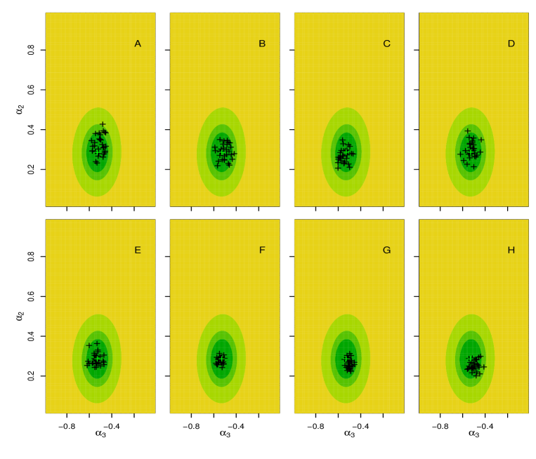
Figure 1: Comparison of different estimators. The likelihood surface for the linear, Gaussian model, with likelihood within $2$ log units of the maximum shown in green, within $4$ log units in light green, within $10$ log units in yellow green, and lower in yellow. The location of the MLE is marked with a green cross. The black crosses show final points from 30 Monte Carlo replications of the estimators: (A) IF1 method; (B) IF2 method; (C) IS2 method; (D) AVIF method ; (E) AVIF method lag 1; (F) AIF method; (G) AIF lag 1 method; (H) Momentum IF method. Each method, was started uniformly over the rectangle shown, with $M=20$ iterations, $N=1000$ particles, and a random walk standard deviation decreasing from $0.02$ geometrically to $0.011$ for both $\alpha_{2}$ and $\alpha_{3}$.

4.2 The Gompertz model

The Gompertz model postulates that the density, $X_{t+\Delta{t}}$, of a population of organisms at time $t+\Delta{t}$ is determined by the density, $X_{t}$, at time $t$ according to

$$X_{t+\Delta{t}}=K^{1-e^{-r\,\Delta{t}}}\,X_{t}^{e^{-r\,\Delta{t}}}\,\varepsilon_{t}.$$ (3)

In equation (3), $K$ is the handling of the population variable, $r$ is a positive parameter, and the $\varepsilon_{t}$ are independent and identically-distributed log-normal random variables with $\log\varepsilon_{t}\sim{\mathrm{Normal}}(0,\sigma^{2})$. In addition, suppose that the population density is measured with some errors which are log-normally distributed:

$$\log{Y_{t}}\;\sim\;{\mathrm{Normal}}\left(\log{X_{t}},\tau^{2}\right).$$ (4)

By transforming into logarithmic scale, we obtain

$$\log{X_{t+\Delta{t}}}\;\sim\;{\mathrm{Normal}}\left(\left(1-e^{-r\,\Delta{t}}\right)\,\log{K}+e^{-r\,\Delta{t}}\,\log{X_{t}},\sigma^{2}\right).$$ (5)

The step to setup gompertz is similar to ou2 model so we skip it and use the default model from pomp by

pompExample(gompertz).

For Gompertz model, the parameters are passed in the argument params and we will estimate them by pmcmc and pmif methods.

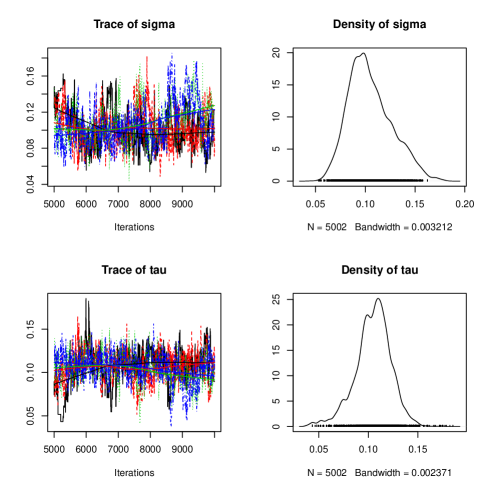
Figure 2: Particle Markov chain Monte Carlo of the Gompertz model (Eqs. 3 and 4). This figure shows the result of the 4 replicated chains of 10000 in length and the burn-in is 5000.

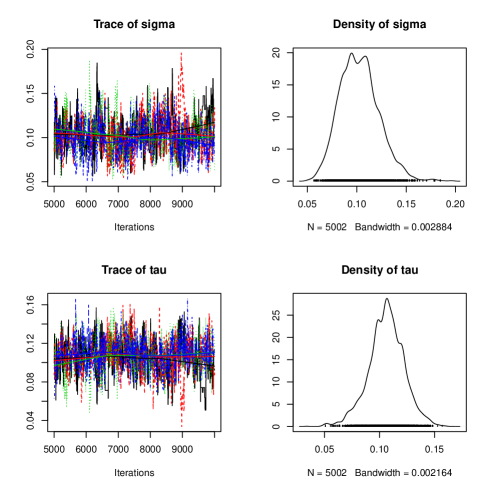
Figure 3: Particle iterated filtering of the Gompertz model (Eqs. 3 and 4). This figure shows the result of the 4 replicated chains of 10000 in length and the burn-in is 5000.

	$ESS(\sigma)$	$ESS(\tau)$
PMCMC	240.4383	296.8016
PMIF	395.3183	583.7596

Table 2: Effective sample size for the gompertz example of 4 replications.

pmcmc <- foreach(
    i=1:4,
    .inorder=FALSE,
    .packages="is2",
    .combine=c,
    .options.multicore=list(set.seed=TRUE)
) %dopar% {
    pmcmc(pomp(gompertz, dprior = gompertz.dprior), start=coef(gompertz),
          Nmcmc = 10000, Np = 100, max.fail = Inf,
          proposal=mvn.diag.rw(c(r = 0.01, sigma = 0.01, tau = 0.01)))
}
######
pmif <- foreach(
    i=1:4,
    .inorder=FALSE,
    .packages="is2",
    .combine=c,
    .options.multicore=list(set.seed=TRUE)
) %dopar% {
    pmif(pomp(gompertz, dprior = gompertz.dprior), start=coef(gompertz),
          Nmcmc = 10000, Np = 100, max.fail = Inf,
          proposal=mvn.diag.rw(c(r = 0.01, sigma = 0.01, tau = 0.01)))
}

It is well known that PMCMC does not mix well for some models (e.g. as observed in (Dahlin et al., 2015b)). By providing extra information through iterated filtering, mixing of the Markov chain can improve significantly. To verify the claim, we compare the performance of PIF with original PMCMC by using diagnostic plots and effective sample size function. Figures 2 and figures 3 show the resulting 5 Markov chains of the PMCMC and PIF algorithms respectively on the left panels and the posterior distributions of each estimated parameters on the right panels. While the diagnostic plot just gives us intuitively visual assessment of the mixing, the MCMC efficiency defined by the effective sample size function clearly demonstrates the effectiveness of pmif over pmcmc (Table 2).

5 A more complex example

Many real world dynamic systems are highly nonlinear, partially observed, and even barely identifiable. To demonstrate the competencies of some of the implemented methodologies for such situations, we apply them to fit a malaria model in North-West India developed by Roy et al. (2012). The reason to choose this challenging model is that it provides a rigorous performance benchmark for our verification.

We follow the setup of Roy et al. (2012) closely. The model we examine divides the investigate population of size $P(t)$ into distinct classes: susceptible individuals, $S(t)$, exposure $E(t)$, infected individuals, $I(t)$, dormant classes $H_{1}(t)$, $H_{2}(t)$, $H_{3}(t)$ and recovered individuals, $Q(t)$. The last $S$ in the model name indicates the possibility that a recovered person can return to the class of susceptible individuals since infection with malaria can lead to incomplete and waning immunity. Data, represented by $y_{1:N}^{*}$, are malaria morbidity reported each month. The state process is

$$\big{(}S(t),E(t),I(t),Q(t),H_{1}(t),H_{2}(t),H_{3}(t),\kappa(t),\mu_{SE}(t)\big{)},$$

where $P(t)$ is from the census data while the birth rate for each class makes sure $S(t)+E(t)+I(t)+Q(t)+\sum_{i}H_{i}(t)=P(t)$ always satisfied. We suppose that $\{X(t),t\geq t_{0}\}$ follows a stochastic differential equation in which the human stage of the malaria pathogen life-cycle is modeled by

$$dS/dt = \delta P+\mathrm{d}P/dt+\mu_{IS}I+\mu_{QS}Q+a\mu_{IH}I+b\mu_{EI}E-\mu_{SE}(t)S-\delta S,$$

$$dE/dt = \mu_{SE}(t)S-\mu_{EI}E-\delta E,$$

$$dI/dt = (1-b)\mu_{EI}E+3\mu_{HI}H_{n}-(\mu_{IH}+\mu_{IS}+\mu_{IQ})I-\delta I,$$

$$dH_{1}/dt = (1-a)\mu_{IH}I-n\mu_{HI}H_{1}-\delta H_{1},$$

$$dH_{i}/dt = 3\mu_{HI}H_{i-1}-3\mu_{HI}H_{i}-\delta H_{i}\hskip 14.22636pt\mbox{for $i\in\{2,3\}$},$$

$$dQ/dt = \mu_{IQ}I-\mu_{QS}Q-\delta Q,$$

where $\delta$ denote mortality rate. Specifically, it represents the average number of deceased people in that class per time unit. In this model, infected population enters dormancy via $I-\mathrm{to}-H$ transition at rate $\mu_{IH}$, and the treated humans join non-relapsing infected in moving to the $\mathrm{Q}$ class. The transition rates from stage $H_{1}$ to $H_{2}$, $H_{2}$ to $H_{3}$ and $H_{3}$ to $Q$ are specified to be $3\mu_{HI}$. The malaria pathogen reproduction within the mosquito vector is specified by

$$\mathrm{d}\kappa/\mathrm{d}t = [\lambda(t)-\kappa(t)]/\tau_{D},$$

$$\mathrm{d}\mu_{SE}/\mathrm{d}t = [\kappa(t)-\mu_{SE}(t)]/\tau_{D}.$$

The latent force of infection $\lambda(t)$ contributes to the current force of infection, $\mu_{SE}(t)$ with mean latency time $\tau_{D}$, after passing through a delay stage, $\kappa(t)$. The relationship between $\lambda(t)$, $\kappa(t)$ and $\mu_{SE}(t)$ can be specified through

$$\mu_{SE}(t)=\int_{-\infty}^{t}\gamma(t-s)\lambda(s)\mathrm{d}s,$$ (6)

with $\gamma(s)=\frac{(2/\tau_{D})^{2}s^{2-1}}{(2-1)!}\exp(-2s/\tau_{D})$, a gamma distribution with shape parameter $2$. As described by Roy et al. (2012), the latent force of infection is given by

$${\lambda(t)=\left(\frac{I+qQ}{P}\right)\times\exp\left\{\sum_{i=1}^{N_{s}}b_{i}s_{i}(t)+b_{r}R(t)\right\}{\times\left[\frac{\mathrm{d}\Gamma(t)}{\mathrm{d}t}\right]}},$$

where $R(t)$ denotes rainfall covariate, $q$ denotes a reduced infection risk from humans in the $\mathrm{Q}$ class and $\{s_{i}(t),i=1,\dots,N_{s}\}$ is a periodic cubic B-spline basis, with $N_{s}=6$. Let initial time $t_{0}=t_{1}-1/12$ and the system is measured at discrete time $t_{1}<t_{2}<\dots<t_{N}$ and the number of new cases in the $n$th interval be $M_{n}=\rho\int_{t_{n-1}}^{t_{n}}[\mu_{EI}E(s)+3\mu_{HI}H_{3}(s)]ds$. Also we assume that $Y_{n}$ given $M_{n}$ follows a negative binomial distribution with mean $M_{n}$ and variance $M_{n}+M_{n}^{2}\sigma^{2}_{\mathrm{obs}}$. We use an Euler-Maruyama scheme (Kloeden and Platen, 1999) with a time step of $1/20$ month to approximate the solution to the above coupled system of stochastic differential equations.

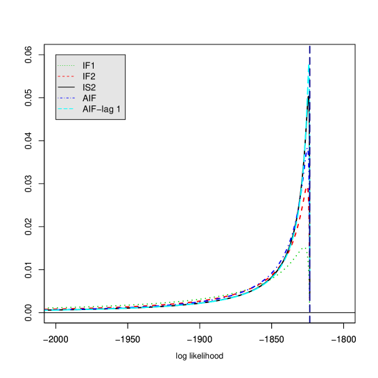
Figure 4: The density of the maximized log-likelihood approximations estimated by IF1, IF2, IS2 and AIF for the malaria model when using J = 1000 and M = 50. The log-likelihood at a previously computed MLE is shown as a dashed vertical line.

Table 3: Summary results of fitting malaria model using IF1, IF2, IS2 and AIF with the number of particle to $J=1000$ and the number of iteration $M=50$.

Algorithms	$\hat{\ell}$	time(s)
IF1	-1904.418	19422.324
IF2	-1879.970	22002.863
IS2	-1870.557	23763.965
AIF	-1861.709	22141.768

We carried out simulation-based inference via the original iterated filtering (IF1), the Bayes map iterated filtering (IF2), second-order iterated smoothing (IS2) and the accelerated iterated filtering (AIF) and AIF with lag 1. The inference goal used to assess all of these methods is to find high likelihood parameter values starting from randomly drawn values in a large hyper-rectangle. We provide this initial hyper-rectangle in the Supplement S-1. In the presence of possible multi-modality, weak identifiability, and considerable Monte Carlo error of this model, we start with about $50$ random searches. We use the standard setting as in (Nguyen and Ionides, 2017) to initially set the random walk standard deviation for estimated parameters to $0.1$ and the cooling rate $c$ to $0.1^{0.02}\approx 0.95$. These corresponding quantities for initial value parameters are set to $2$ and $0.1^{0.02}$, respectively. We run our experiment on a computer node with $M=50$ iterations and with $J=1000$ particles. The chosen values are reasonable for exploring the likelihood surface of this model since increasing the iterations and the number of particles does not improve the results much and it significantly takes longer time. Figure 4 shows the the MLEs estimated by IF1, IF2, IS2 and AIF. Higher mean and smaller variance of the MLEs, our implemented methods demonstrate that they are considerably more effective than IF1. Table 3 shows the summary of the estimate likelihood and computational time. Note that the computational times for IF1, IF2, IS2 and AIF are 19422.324, 22002.863, 23763.965 and 22141.768 seconds respectively, confirming that all proposed methods have essentially the same computational cost as the first order methods for a given Monte Carlo sample size and number of iterations. While IF1 reveals their limitations in this challenging problem, we have shown that IF2 and all new methods can still offer a substantial improvement over IF1. Additional illustrations confirm it can be found online.

6 Conclusion

The is2 package is designed to be a useful tool for time series modeling and analysis of POMP models so that it is painless to make inference via open-source software. Inherited robust platform from pomp package, a large set of of inference are made available to practical researchers, freeing them from writing their own code from scratch. Moreover, model specification language focused on modeling domain, separating from the inference method, facilitates model selection at the design stage. The examples demonstrated in this paper are well represented the potential of the package in a number of scientific studies.

As an open-source project, is2 is especially convenient for carrying out algorithms with the plug-and-play property, since models will typically be specified by their rprocess simulator, together with rmeasure. The package is easily extendable for simulation and computationally efficient data analysis in various ways: for example, different sampling could be added to the package. In addition, while we focused on plug-and-play methodss, inference approaches for non-plug-and-play can be added by building on generic inference packages such as NIMBLE (de Valpine et al., 2017) or STAN (Carpenter et al., 2017). Advances in improving the current class of inferences play an important part of the statistical machinery for time series models, potentially applicable beyond dynamic modeling.

Efficiency and scalability are necessary component of any modern software packages. Currently, is2 provides users with key functions written in C and embarrassingly parallel computations. It is possible to embed parallelization to increase the performance for certain computationally intensive tasks but we leave it for our future work.

To sum up, is2 is currently effective for estimating numerous types of infectious disease models, and the fixed lag smoothing component allows researchers to employ the different sampling or resampling schemes in any desired models. As additional features are augmented, we expect that the package keeps pace with pomp as a supplementary set of tools for pomp computation and study. Last but not least, more examples, which can be used as templates for implementation of new models; the R and C code underlying these examples are provided with the package. In addition, documentation and an introductory vignette are provided with the package and on the is2 website http://github.com/nxdao2000/is2.

Acknowledgements

This research is funded in part by the University of Mississippi Summer Grant.

References

- Andrieu et al. (2010) Andrieu C, Doucet A, Holenstein R (2010). “Particle Markov Chain Monte Carlo.” Journal of the Royal Statistical Society B, 72(3), 269–342. 10.1111/j.1467-9868.2009.00736.x.
- Andrieu and Roberts (2009) Andrieu C, Roberts GO (2009). “The Pseudo-Marginal Approach for Efficient Computation.” The Annals of Statistics, 37(2), 697–725. 10.1214/07-AOS574.
- Andrieu et al. (2015) Andrieu C, Vihola M, et al. (2015). “Convergence properties of pseudo-marginal Markov chain Monte Carlo algorithms.” The Annals of Applied Probability, 25(2), 1030–1077.
- Andrieu et al. (2016) Andrieu C, Vihola M, et al. (2016). “Establishing some order amongst exact approximations of MCMCs.” The Annals of Applied Probability, 26(5), 2661–2696.
- Bretó et al. (2009) Bretó C, He D, Ionides EL, King AA (2009). “Time Series Analysis via Mechanistic Models.” The Annals of Applied Statistics, 3, 319–348. 10.1214/08-AOAS201.
- Cappé et al. (2007) Cappé O, Godsill S, Moulines E (2007). “An Overview of Existing Methods and Recent Advances in Sequential Monte Carlo.” Proceedings of the IEEE, 95(5), 899–924. 10.1109/JPROC.2007.893250.
- Carpenter et al. (2017) Carpenter B, Gelman A, Hoffman MD, Lee D, Goodrich B, Betancourt M, Brubaker M, Guo J, Li P, Riddell A (2017). “Stan: A probabilistic programming language.” Journal of Statistical Software, 76(1).
- Dahlin et al. (2015a) Dahlin J, Lindsten F, Kronander J, Schön TB (2015a). “Accelerating pseudo-marginal Metropolis-Hastings by correlating auxiliary variables.” arXiv preprint arXiv:1511.05483.
- Dahlin et al. (2015b) Dahlin J, Lindsten F, Schön TB (2015b). “Particle Metropolis–Hastings using gradient and Hessian information.” Statistics and Computing, 25(1), 81–92.
- Dauphin et al. (2014) Dauphin YN, Pascanu R, Gulcehre C, Cho K, Ganguli S, Bengio Y (2014). “Identifying and attacking the saddle point problem in high-dimensional non-convex optimization.” In Advances in Neural Information Processing Systems, pp. 2933–2941.
- de Valpine et al. (2017) de Valpine P, Turek D, Paciorek CJ, Anderson-Bergman C, Lang DT, Bodik R (2017). “Programming with models: writing statistical algorithms for general model structures with NIMBLE.” Journal of Computational and Graphical Statistics, 26(2), 403–413.
- Del Moral (2004) Del Moral P (2004). Feynman-Kac Formulae: Genealogical and Interacting Particle Systems with Applications. Springer-Verlag, New York.
- Dippon and Renz (1997) Dippon J, Renz J (1997). “Weighted means in stochastic approximation of minima.” SIAM Journal on Control and Optimization, 35(5), 1811–1827.
- Doucet et al. (2000) Doucet A, Godsill S, Andrieu C (2000). “On sequential Monte Carlo sampling methods for Bayesian filtering.” Statistics and Computing, 10(3), 197–208.
- Doucet et al. (2013) Doucet A, Jacob PE, Rubenthaler S (2013). “Derivative-free estimation of the score vector and observed information matrix with application to state-space models.” arXiv preprint arXiv:1304.5768.
- Ghadimi and Lan (2016) Ghadimi S, Lan G (2016). “Accelerated gradient methods for nonconvex nonlinear and stochastic programming.” Mathematical Programming, 156(1-2), 59–99.
- Ionides et al. (2011) Ionides EL, Bhadra A, Atchadé Y, King AA (2011). “Iterated Filtering.” The Annals of Statistics, 39(3), 1776–1802. 10.1214/11-AOS886.
- Ionides et al. (2006) Ionides EL, Bretó C, King AA (2006). “Inference for Nonlinear Dynamical Systems.” Proceedings of the National Academy of Sciences of the USA, 103(49), 18438–18443. 10.1073/pnas.0603181103.
- Ionides et al. (2015) Ionides EL, Nguyen D, Atchadé Y, Stoev S, King AA (2015). “Inference for dynamic and latent variable models via iterated, perturbed Bayes maps.” Proceedings of the National Academy of Sciences of the USA. 10.1073/pnas.1410597112.
- King et al. (2014) King AA, Ionides EL, Bretó CM, Ellner SP, Ferrari MJ, Kendall BE, Lavine M, Nguyen D, Reuman DC, Wearing H, Wood SN (2014). \pkgpomp: Statistical Inference for Partially Observed Markov Processes. \proglangR package, version 0.53-1, URL http://pomp.r-forge.r-project.org.
- King et al. (2015) King AA, Nguyen D, Ionides EL (2015). “Statistical inference for partially observed Markov processes via the R package pomp.” arXiv preprint arXiv:1509.00503.
- Kitagawa (1996) Kitagawa G (1996). “Monte Carlo filter and smoother for non-Gaussian nonlinear state space models.” Journal of Computational and Graphical Statistics, 5(1), 1–25.
- Kitagawa (1998) Kitagawa G (1998). “A Self-organising State Space Model.” Journal of the American Statistical Association, 93, 1203–1215. 10.1080/01621459.1998.10473780.
- Kloeden and Platen (1999) Kloeden PE, Platen E (1999). Numerical Soluion of Stochastic Differential Equations. 3rd edition. Springer, New York.
- Kushner (2010) Kushner H (2010). “Stochastic approximation: a survey.” Wiley Interdisciplinary Reviews: Computational Statistics, 2(1), 87–96.
- Kushner and Clark (2012) Kushner HJ, Clark DS (2012). Stochastic approximation methods for constrained and unconstrained systems, volume 26. Springer Science & Business Media.
- Kushner and Yang (1993) Kushner HJ, Yang J (1993). “Stochastic approximation with averaging of the iterates: Optimal asymptotic rate of convergence for general processes.” SIAM Journal on Control and Optimization, 31(4), 1045–1062.
- LeCun et al. (2012) LeCun YA, Bottou L, Orr GB, Müller KR (2012). “Efficient backprop.” In Neural networks: Tricks of the trade, pp. 9–48. Springer.
- Lindström (2013) Lindström E (2013). “Tuned iterated filtering.” Statistics & Probability Letters, 83(9), 2077–2080.
- Liu and West (2001) Liu J, West M (2001). “Combining Parameter and State Estimation in Simulation-Based Filtering.” In A Doucet, N de Freitas, NJ Gordon (eds.), Sequential Monte Carlo Methods in Practice, pp. 197–224. Springer-Verlag, New York.
- Nemeth et al. (2016a) Nemeth C, Fearnhead P, Mihaylova L (2016a). “Particle approximations of the score and observed information matrix for parameter estimation in state–space models with linear computational cost.” Journal of Computational and Graphical Statistics, 25(4), 1138–1157.
- Nemeth et al. (2016b) Nemeth C, Sherlock C, Fearnhead P (2016b). “Particle Metropolis-adjusted Langevin algorithms.” Biometrika, 103(3), 701–717.
- Nesterov (2005) Nesterov Y (2005). “Smooth minimization of non-smooth functions.” Mathematical Programming, 103(1), 127–152.
- Nesterov (2013) Nesterov Y (2013). Introductory lectures on convex optimization: A basic course, volume 87. Springer Science & Business Media.
- Nguyen (2018) Nguyen D (2018). “Accelerate iterated filtering.” ArXiv Preprint arXiv:1802.08613.