Quantum Kerr oscillators’ evolution in phase space: Wigner current,
symmetries, shear suppression and special states

Abstract

The creation of quantum coherences requires a system to be anharmonic. The simplest such continuous one-dimensional quantum system is the Kerr oscillator. It has a number of interesting symmetries we derive. Its quantum dynamics is best studied in phase space, using Wigner’s distribution $W$ and the associated Wigner phase space current ${\mathbf{J}}$. Expressions for the continuity equation governing its time evolution are derived in terms of ${\mathbf{J}}$ and it is shown that ${\mathbf{J}}$ for Kerr oscillators follows circles in phase space. Using ${\mathbf{J}}$ we also show that the evolution’s classical shear in phase space is quantum suppressed by an effective “viscosity”. Quantifying this shear suppression provides measures to contrast classical with quantum evolution and allows us to identify special quantum states.

I Introduction

The formation of quantum coherences is of central importance in the study of quantum systems and their dynamics.

Here we consider closed one-dimensional Kerr-type oscillators. These are anharmonic and can therefore create coherences Kakofengitis et al. (2017). Additionally, their dynamics has circular symmetry in phase space. This makes them the simplest continuous system to create coherences.

In other words, the results reported here apply to regular anharmonic systems (with Hamiltonians of the form $\hat{H}=\hat{p}^{2}/2m+V(\hat{x})$, see Oliva et al. (2017) and Oliva and Steuernagel (2019)) but the Kerr-oscillators’ symmetries make them particularly suited to help us understand aspects of nonclassical effects in quantum dynamics.

Wigner’s distribution $W$ Wigner (1932); Hillery et al. (1984) is the closest quantum analog Zurek (2001); Oliva et al. (2017); Hillery et al. (1984); Leibfried et al. (1998); Tilma et al. (2016) of the classical phase space distribution $\rho$. In continuous one-dimensional systems the creation of quantum coherences is represented by the creation of negative regions of the Wigner distribution Heller (1976); Feynman (1987); Leibfried et al. (1998); Zurek (2001); Oliva et al. (2017). The formation of such negative regions in the Wigner distribution is easily monitored numerically.

The evolution of $W$ is governed by the associated Wigner phase-space current ${\mathbf{J}}$ (strictly speaking ${\mathbf{J}}$ is a probability current density). Generally, phase-space-based approaches are suitable for comparison of quantum with classical dynamics Berry and Balazs (1979); Zurek (2001); Oliva and Steuernagel (2019). Specifically, ${\mathbf{J}}$ allows us to adopt a geometric approach Steuernagel et al. (2013); Kakofengitis and Steuernagel (2017); Kakofengitis et al. (2017); Oliva et al. (2017); Oliva and Steuernagel (2019) to studying quantum dynamics.

We introduce Kerr oscillators, their Wigner distribution $W$, and their associated Wigner current ${\mathbf{J}}$ in Sec. II. In Sec. III we show that there are no trajectories and no phase-space flow for anharmonic systems such as Kerr oscillators. In Sec. IV we investigate how pulses in phase space smear out classical spirals [Fig. 1(b); in all figures atomic units with $\hbar=1$, $M=1$ and $k=1$ are used]. We find that pulses in phase space steepen and lengthen dynamically. This analysis is aided by the system’s circular symmetry and the fact that the probability on circles in phase space is conserved. In Sec. V we show that using Wigner current ${\mathbf{J}}$’s effective “viscosity” Oliva and Steuernagel (2019) allows us to contrast classical with quantum dynamics and pick out special quantum states.

Our results can be generalised to higher-dimensional systems Wigner (1932).

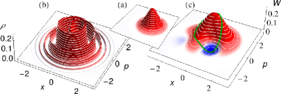
Figure 1: Probability distributions in phase space.(a), We start from a weakly excited coherent state $|\alpha\rangle=|7/12\rangle$ which is positive everywhere.(b), After time $t=60$ under classical time evolution, $\rho(t)$ has formed a highly sheared and tight spiral.(c), After the same time the quantum evolution yields a Wigner distribution $W(t)$ which has much less fine detail but negativities (blue). The green line superimposed on(c) traces out the Wigner distribution profile on a ring around the origin with radius $r=1$ which passes through an area with pronounced negativity. Fig. 2 displays evolution on this ring [$\Lambda=\frac{1}{2}$, see Eq. (4)].

II Wigner distributions and Wigner current of Kerr oscillators

A one-dimensional system’s Wigner distribution $W_{\varrho}(x,p,t)$ Wigner (1932); Hillery et al. (1984) (where $x$ denotes position, $p$ the associated momentum, and $t$ time), for a quantum state described by a density matrix $\hat{\varrho}$, is defined as the Fourier transform of its off-diagonal coherences $\varrho(x+y,x-y,t)$ (parametrized by the shift $y$)

$$W_{\varrho}(x,p,t)=\frac{1}{\pi\hbar}\int_{-\infty}^{\infty}dy\;\langle x+y|\hat{\varrho}(t)|x-y\rangle\;e^{-\frac{2i}{\hbar}py},\quad$$ (1)

where $\hbar=h/(2\pi)$ is Planck’s constant. By construction $W$ is normalized and nonlocal (through $y$). Unlike $\hat{\varrho}$, $W$ is always real-valued but, generically, $W$ features negativities Wigner (1932). Since $W_{\varrho}$ is $\hat{\varrho}$’s Fourier transform, $W$ and $\hat{\varrho}$ are isomorphic to each other, allowing us to describe all aspects of the quantum system’s state and its dynamics using the Wigner representation of quantum theory Zachos et al. (2005).

II.1 Time evolution of the Wigner distribution

For conservative Kerr systems the time development of $W$ is given by the Moyal-bracket $\{\{.,.\}\}$ Moyal (1949); Zachos et al. (2005)

$$\partial_{t}W(x,p,t)=\{\{H,W\}\}\$$ (2)

$$\;\equiv\frac{2}{\hbar}~{}H(x,p)\ \sin\left({{\tfrac{\hbar}{2}}(\stackrel{{\scriptstyle\leftarrow}}{{\partial}}_{x}\stackrel{{\scriptstyle\rightarrow}}{{\partial}}_{p}-\stackrel{{\scriptstyle\leftarrow}}{{\partial}}_{p}\stackrel{{\scriptstyle\rightarrow}}{{\partial}}_{x})}\right)\ W(x,p,t).$$ (3)

Here, $\partial_{x}=\frac{\partial}{\partial x}$, etc.; the arrows over the derivatives indicate whether they act on (point towards) Hamiltonian or Wigner distribution.

The Hamiltonian of anharmonic single-mode oscillators of the Kerr type has the form

$${\hat{H}}_{\Lambda}=\left(\frac{\hat{p}^{2}}{2M}+\frac{k}{2}\hat{x}^{2}\right)+\Lambda^{2}\left(\frac{\hat{p}^{2}}{2M}+\frac{k}{2}\hat{x}^{2}\right)^{2},$$ (4)

with the oscillator mass $M$ and spring constant $k$. Such Hamiltonians describe electromagnetic fields subjected to Kerr nonlinearities $\chi^{(3)}$ (here $\Lambda^{2}\propto{\chi^{(3)}}$) Walls and Milburn (1994); Osborn and Marzlin (2009); Man’ko et al. (2010); Kirchmair et al. (2013). This system is fully solvable since wave functions of the harmonic oscillator are solutions to the Kerr Hamiltonian with eigenenergies $E_{n}=\hbar\sqrt{\frac{k}{M}}[(n+\frac{1}{2})+\Lambda^{2}(n+\frac{1}{2})^{2}]$. Its quantum recurrence time is

$$T_{\Lambda}=\frac{\pi}{|\Lambda|^{2}}.$$ (5)

Following Wigner Wigner (1932), we cast expression (3) in the form of the phase-space continuity equation

$$\partial_{t}W+\bm{\nabla}\cdot{{\mathbf{J}}}=0\;,$$ (6)

$$\mbox{ where }\bm{\nabla}=\genfrac{(}{)}{0.0pt}{}{\partial_{x}}{\partial_{p}}\mbox{ is the gradient, and }{{\mathbf{J}}}=\genfrac{(}{)}{0.0pt}{}{J_{x}}{J_{p}}$$

denotes the Wigner current in phase space Steuernagel et al. (2013). ${\mathbf{J}}$ is the quantum analog Donoso and Martens (2001); Bauke and Itzhak (2011) of the classical phase-space current ${\mathbf{j}}=\rho{\mathbf{v}}$ Nolte (2010) which transports the classical probability density $\rho(x,p,t)$ according to Liouville’s continuity equation $\partial_{t}\rho=-{\bm{\nabla}}\cdot{\mathbf{j}}$.

${{\mathbf{J}}}$ reveals details Steuernagel et al. (2013); Kakofengitis and Steuernagel (2017) about quantum systems’ phase space dynamics previously thought inaccessible due to the supposed “blurring” by Heisenberg’s uncertainty principle.

From now on we will consider $M=k=1$ only. Then [for a derivation see Eqs. (22) and (23) in the Appendix VI], with ${{\mathbf{r}}}=(x,p)=r(\cos\theta,\sin\theta)$, $r=\sqrt{x^{2}+p^{2}}$ and $\bm{\Delta}=\partial_{x}^{2}+\partial_{p}^{2}$, ${{\mathbf{J}}}$ can be written as

$${{\mathbf{J}}} =\genfrac{(}{)}{0.0pt}{}{p}{-x}\left[1+\Lambda^{2}\left(x^{2}+p^{2}-{\frac{\hbar^{2}}{4}}\bm{\Delta}\right)\right]W=\genfrac{(}{)}{0.0pt}{}{r\sin\theta}{-r\cos\theta}\left[1+\Lambda^{2}\left(r^{2}-{\frac{\hbar^{2}}{4}}(\partial_{r}^{2}+\frac{1}{r}\partial_{r}+\frac{1}{r^{2}}\partial_{\theta}^{2})\right)\right]W\;.$$ (7)

${{\mathbf{J}}}$ is tangent to circles concentric with the origin of phase space. This circular symmetry allows us to consider an approximation of the dynamics on such individual circles, an observation we make use of below.

For future reference we split ${\mathbf{J}}$ into its classical ${\mathbf{j}}$ and quantum terms ${\mathbf{J}}^{Q}$

$${{\mathbf{J}}} ={\mathbf{j}}+{\mathbf{J}}^{Q}=W{\mathbf{v}}-\genfrac{(}{)}{0.0pt}{}{p}{-x}\left({\frac{\hbar^{2}\Lambda^{2}}{4}}\bm{\Delta}\right)W.$$ (8)

Here ${\mathbf{v}}=\genfrac{(}{)}{0.0pt}{}{p}{-x}(1+\Lambda^{2}r^{2})$ is the classical phase-space velocity. The quantum terms ${\mathbf{J}}^{Q}$ are only present for anharmonic potentials Kakofengitis et al. (2017), which is why only anharmonic potentials create coherences. Harmonic systems’ phase-space dynamics follows ${\mathbf{v}}$ and is classical, see Refs. Oliva et al. (2017); Kakofengitis et al. (2017).

III No trajectories or flow in quantum phase space

Inspired by classical mechanics, there have been several attempts to treat quantum phase-space evolution as a flow along trajectories Oliva et al. (2017). Such attempts are ill fated Oliva et al. (2017) as we explain now. They use the formal factorization ${\mathbf{J}}=W{\mathbf{w}}$ to define a “quantum phase-space velocity” ${\mathbf{w}}={\mathbf{J}}/W$, then the continuity equation (6) assumes the form Trahan and Wyatt (2003); Daligault (2003); Oliva et al. (2017)

$$\partial_{t}W+{\mathbf{w}}\cdot\bm{\nabla}W+W\bm{\nabla}\cdot{\mathbf{w}}=0\;.$$ (9)

Here the convective term ${\mathbf{w}}\cdot\bm{\nabla}W$ describes the transport that carries $W$ along with the current (following fieldlines in phase space) without changing its values. In contrast, the current divergence term $W\bm{\nabla}\cdot{\mathbf{w}}$ changes values of $W$. This is best seen by formally rearranging Eq. (9) for the total derivative

$$\frac{dW}{dt}=\partial_{t}W+{\mathbf{w}}\cdot\bm{\nabla}W=-W\bm{\nabla}\cdot{\mathbf{w}}\;.$$ (10)

Treating a continuity equation in this form is known as its Lagrange decomposition. This decomposition has to be treated with extreme caution, since it essentially splits the well behaved and finite term $\bm{\nabla}\cdot\bm{J}$ into the two individually singular terms ${\mathbf{w}}\cdot\bm{\nabla}W$ and $W\bm{\nabla}\cdot\bm{w}$. Some implications are discussed below.

For the Kerr system this total derivative is

$$\frac{dW}{dt} =-\frac{\Lambda^{2}\hbar^{2}}{4}\left[p\left(\frac{(\partial_{x}W)}{W}-\partial_{x}\right)\right.\left.-x\left(\frac{(\partial_{p}W)}{W}-\partial_{p}\right)\right]\bm{\Delta}W=-\frac{\Lambda^{2}\hbar^{2}}{4}W\partial_{\theta}\left(\frac{\bm{\Delta}W}{W}\right),$$ (11)

and the convective transport term in Eq. (10) is

$${\mathbf{w}}\cdot\bm{\nabla}W=\left(\Lambda^{2}\left[-r^{2}+\frac{\hbar^{2}}{4W}\bm{\Delta}W\right]-1\right)\partial_{\theta}W.$$ (12)

Since the divergence $\bm{\nabla}\cdot{\mathbf{w}}$ is nonzero, the quantum evolution does not preserve phase-space volumes Moyal (1949); Kakofengitis et al. (2017); Oliva et al. (2017).

One could still describe quantum evolution by phase-space transport if the magnitude of this divergence were finite across the entire phase space Oliva et al. (2017). Indeed, modelling quantum phase-space dynamics through such transport along trajectories has been attempted many times; in this context it has been considered an undesirable feature of ${\mathbf{w}}$ that it is a singular quantity when $W$ is zero (see Ref. Oliva et al. (2017) for details). But zeros in $W$ are unavoidable Hudson (1974):

The singularities in $\bm{\nabla}\cdot{\mathbf{w}}$ are a fundamental and necessary feature to create negative regions in $W$ and thus to create quantum coherences. Such singularities are not a flaw. A velocity field ${\mathbf{w}}$ with positive divergence that is bounded from above, $B>\bm{\nabla}\cdot{\mathbf{w}}>0$, will by itself not be able to generate negativities. The associated expansion of phase-space volumes can only reduce the initial value $W(0)>0$ of a density towards zero, since Eq. (10) implies that Trahan and Wyatt (2003); Oliva et al. (2017)

$$W(t)|_{\text{comoving}}>W(0)\exp(-Bt)>0$$ (13)

for all times. Trahan and Wyatt noticed this and concluded that “the sign of the density riding along the trajectory cannot change” Trahan and Wyatt (2003).

But this interpretation is incorrect. When $W=0$ the velocity ${\mathbf{w}}$ and its divergence is singular, Eq. (11) cannot be integrated since ${\mathbf{w}}$’s singularities render integrals and associated bounds such as (13) ill-defined Oliva et al. (2017). Therefore, in anharmonic quantum systems neither trajectories nor transport along flow lines exist Oliva et al. (2017). (Refs. Bauke and Itzhak (2011) and Steuernagel et al. (2013) refer to Wigner “flow” but were written before this was realized.)

Because of the singular volume changes associated with Eq. (11), we feel the quantum Liouville equation (6) should be called Wigner’s continuity equation instead.

We are forced to conclude that a trajectory-based approach to quantum phase-space evolution creates contradictions such as singular ${\mathbf{w}}$ and singular phase-space volume changes. This highlights the stark differences between classical and quantum dynamics in an illuminating manner. The singularities in ${\mathbf{w}}$ and phase-space volume changes are needed to violate inequality (13) thus allowing for the creation of quantum coherences and negative regions in $W$ Kakofengitis et al. (2017); Oliva et al. (2017).

IV Pulses in Quantum phase space

In the classical case the probability (of $\rho$) on a classical trajectory of a conservative system is conserved over time. It can be checked that the probability (of $W$) on a classical trajectory is not conserved for typical anharmonic quantum systems.

The quantum Kerr system is an exception as its evolution preserves probability on rings around the origin:

$$\ointctrclockwise d\theta\;\;\partial_{t}W=-\ointctrclockwise d\theta\;\;\bm{\nabla}\cdot{{\mathbf{J}}}=0,$$ (14)

since $\bm{\nabla}\cdot{\bm{J}}=r\partial_{\theta}([v(r)-\Lambda^{2}\frac{\hbar^{2}}{4}\bm{\Delta}]W)$. In addition to the circular symmetry displayed in Eq. (7), this probability conservation on circles is the primary reason why considering the Kerr dynamics on circles is suitable.

The classical velocity profile $v(r)$ leads to the formation of fine detail in the classical evolution: in the case of a Gaussian initial state, the state becomes wrapped into a single tightly wound spiral [see Fig. 1(b)]. The quantum evolution shows this tendency of spiral wrapping as well, but while the formation of fine detail is suppressed through “viscous” behaviour (see Sec. V), negativities of the Wigner distribution emerge. To study this in more detail, consider $W$ on a ring of radius $r$, as displayed in Fig. 2.

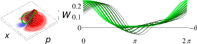
Figure 2: Time evolution of $W(\theta)$ on a ring with fixed radius $r=1.0$ for initial coherent state $|\alpha\rangle=|7/12\rangle$ over time $t=0$ to $T_{\Lambda}/4=4\pi=12.56$ [$\Lambda=\frac{1}{4}$]. The darker and thinner the curves, the more time has elapsed. The curves move clockwise on the ring, towards increasing values of “$-\theta$”. The quantum evolution leads to a speedup over the classical evolution (the classical phase angle $vt$ is subtracted). Additionally, under quantum evolution the pulse widens and steepens at the front, this triggers the formation of oscillations with negative regions in front of the pulse which eventually catch up with the main pulse from “behind”.

The quantum “cross-talk” terms $\partial_{r}^{2}+\frac{1}{r}\partial_{r}$ in Eq. (7) couple the current on adjacent rings. We can cast these terms aside if we may assume that the Wigner distribution’s azimuthal curvature $\partial_{\theta}^{2}W$ is much greater than its radial curvature and gradient. Making this assumption temporarily, the velocity on a ring is approximately

$$w(r,\theta)\approx r\left[1+\Lambda^{2}\left(r^{2}-{\frac{\hbar^{2}}{4r^{2}}}\frac{1}{W}\partial_{\theta}^{2}W\right)\right].$$ (15)

This approximation is obviously poor when $W\approx 0$, but Eq. (15) is still useful for the discussion that follows.

In Figs. 2-4 the full evolution is portrayed, not its approximate behaviour of Eq. (15). The axis “$-\theta$” is chosen in Figs. 2-4 since classical evolution proceeds clockwise, in the direction of negative values of $\theta$.

The effect of the $\theta$-curvature term, retained in Eq. (15), is primarily twofold: for a Wigner distribution on a circle, forming a hump, the hump’s leading and trailing edges, having positive curvature, get delayed. Conversely, the negative curvature of the peak of the hump accelerates its center (see Fig. 2). This lengthens the pulse, making the tail trail, and sharpens its front since the center catches up with the front (see Fig. 2). This sharpening in turn spawns oscillations that project forward from the pulse (see Fig. 2 and discussion in Ref. Friedman and Blencowe (2017)).

A narrower pulse, as portrayed in Fig. 3, develops more pronounced oscillations. Additionally, in Fig. 3, $\Lambda$ is chosen formally complex such that $\Lambda^{2}_{-}<0$. This creates “backwards” dynamics when contrasted with a positive Kerr-nonlinearity (compare Figs. 2 and 3: in Fig. 3 the pulse lengths to the “right” and steepens and spawns oscillations to the “left”; in “reverse” to Fig. 2).

In Fig. 4, two pulses on a ring interfere with each other. Here, like in Fig. 2, the overall effect is that the quantum terms speed the pulses up.

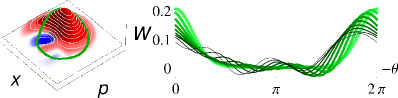
Figure 3: Time evolution of $W(\theta)$ on a ring with fixed radius $r=1.6$ for initial coherent state $|\alpha\rangle=|5/4\rangle$ over time $t=0$ to $T_{\Lambda_{-}}/4=12.56$. Here the Kerr-nonlinearity is negative, $\Lambda_{-}^{2}=-1/16$, therefore the Wigner distribution is wrapped anticlockwise and the center of gravity of the pulse falls behind the classical motion ($vt$ has been subtracted). Contrast with Fig. 2.

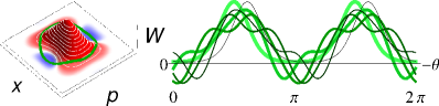
Figure 4: Time evolution of $W(\theta)$ on a ring with fixed radius $r=1.6$ for initial squeezed vacuum state (squeezing parameter $=1/3$) over time $t=0$ to $T_{\Lambda_{+}}=\frac{\pi}{4}=0.785$. Here the Kerr-nonlinearity is positive, $\Lambda_{+}^{2}=1$, therefore the Wigner distribution’s center of gravity moves ahead of the classical motion ($vt$ has been subtracted): at time $t=\frac{T_{1}}{4}$ (its recurrence time is shortened by $\frac{T_{1}}{4}$ because the squeezed state is symmetric with respect to the origin) the original pulse reforms and is rotated forward, similar to Fig. 2.

V ${\mathbf{J}}$’s viscosity and special states

In Sec. IV we discussed motion on a ring. Here we consider cross talk between motion on neighbouring rings.

Over time classical Hamiltonian phase-space flow shears $\rho$ since ${\mathbf{v}}$ creates nonzero gradients of its angular velocity across energy shells. This flow is inviscid as ${\mathbf{v}}$ is independent of $\rho$; thus no terms suppress the effects of the angular velocity gradients, and, as time progresses, nonsingular probability distributions in phase space get sheared into ever finer filaments [see Fig. 1(b)].

The associated classical phase-space shear has been derived in Ref. Oliva and Steuernagel (2019) as

$$s(x,p;H)=\partial_{\widehat{{\bm{\nabla}}}_{\!\!H}}(-{\bm{\nabla}}\times{\mathbf{v}})=\partial_{\widehat{{\bm{\nabla}}}_{\!\!H}}(\partial_{p}v_{x}-\partial_{x}v_{p}).$$ (16)

Here the directional derivative across energy shells, $\partial_{\widehat{{\bm{\nabla}}}_{\!\!H}}$, is formed from the normalized gradient $\widehat{\bm{\nabla}}_{\!\!H}={\bm{\nabla}}H/|{\bm{\nabla}}H|$ of the Hamiltonian $H$. Because of the Kerr system’s circular symmetry, $\widehat{\bm{\nabla}}_{\!\!H}=\partial_{r}$.

The sign convention using the negative curl in $s$ in Eq. (16) is designed to yield a positive sign for clockwise-orientated fields since this is the prevailing direction of the classical velocity field ${\mathbf{v}}$. This choice yields $s>0$ for hard potentials (potentials for which the magnitude of the force increases with increasing amplitude, i.e., $\Lambda^{2}>0$), since they induce clockwise shear [see Fig. 1(b)]. $s=0$ for harmonic oscillators (i.e., $\Lambda=0$), and $s<0$ for soft potentials (for which the magnitude of the force decreases with increasing amplitude, i.e., $\Lambda^{2}<0$) since they induce anticlockwise shear.

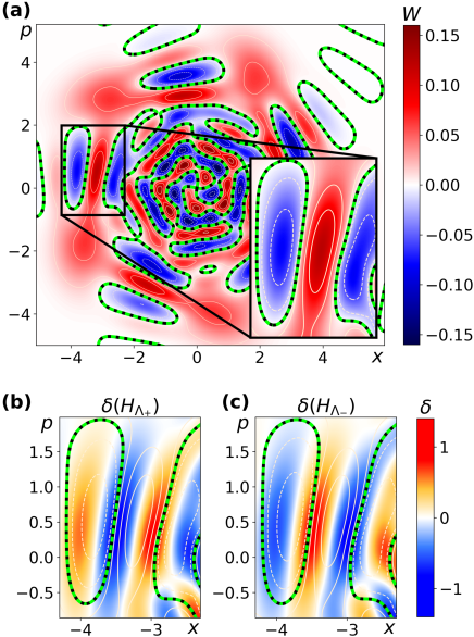
Figure 5: Polarization of the vorticity $\delta$ and inversion of this polarization. (a), The Wigner distribution $W$ of a Gaussian initial state centered on $x=-4$, $p=0$ and evolved to $t=40$ using $\hat{H}_{\Lambda_{+}}=\hat{H}_{{1}/{4}}$. Its contours (for emphasis the zero contour is shown as black-green dashed lines) are also employed in (b) and (c). The inset for $W$ in (a) is reproduced showing the effects of,(b), clockwise shear [$\delta(H_{\Lambda_{+}})$] and,(c), anticlockwise shear [$\delta(H_{\Lambda_{-}})$]. Comparing (b) with (c) demonstrates polarization inversion of $\delta$ associated with shear inversion of the system, here $\Lambda^{2}_{+}=+(1/4)^{2}=-\Lambda^{2}_{-}$.

The reaction of quantum dynamics to classical shear $s$ has to reside in ${\mathbf{J}}^{Q}$ of Eq. (8). To extract it we form the vorticity of ${\mathbf{J}}^{Q}$ Oliva and Steuernagel (2019):

$$\delta(x,p,t;H)=-{\bm{\nabla}}\times{\mathbf{J}}^{Q}=\partial_{p}J_{x}^{Q}-\partial_{x}J_{p}^{Q}\;.$$ (17)

$\delta$’s sign distribution shows a pronounced polarization pattern, see Fig. 5.

Specifically, for a system with clockwise shear Fig. 5(b) illustrates that $\delta(H_{\Lambda_{+}})$ [with $\Lambda^{2}_{+}=+(1/4)^{2}$] tends to be positive on the inside (towards the origin) and negative on the outside of the positive main ridge of $W$ [see inset of Fig. 5(a)]. Because of this, the outside is being slowed down while the inside speeds up. This polarized distribution of $\delta$ therefore counteracts the classical shear ($s_{H_{\Lambda_{+}}}>0$) and can suppress it altogether Oliva and Steuernagel (2019). The same applies to other positive regions of $W$, whereas for its negative regions the current ${\mathbf{J}}$ tends to be inverted Steuernagel et al. (2013); Kakofengitis and Steuernagel (2017), inverting $\delta$’s polarization pattern [see Ref. Oliva and Steuernagel (2019) and Fig. 5(b)].

When the same state $W$ is governed by a Hamiltonian $H_{\Lambda_{-}}$ with anticlockwise shear Oliva and Steuernagel (2019) [i.e., $(\Lambda_{-})^{2}<0$], $\delta(H_{\Lambda_{-}})$ tends to be the sign-inverted form of $\delta(H_{\Lambda_{+}})$ (for Kerr systems we find $\delta(H_{\Lambda_{+}})=-\delta(H_{\Lambda_{-}})$ if $|\Lambda_{+}|=|\Lambda_{-}|$). This is illustrated in Fig. 5(c), where $\Lambda^{2}_{-}=-(1/4)^{2}$ is negative, whereas in Fig. 5(b) $\Lambda^{2}_{+}=+(1/4)^{2}$ is positive.

The distribution of $\delta$’s polarization can be picked up with the directional derivative $\partial_{\widehat{{\bm{\nabla}}}_{\!\!H}}\delta(t;H)=\partial_{r}\delta(t;H)$. This we multiply with $W$, because negative regions of $W$ invert the current ${\mathbf{J}}$ Steuernagel et al. (2013), and because we want to weight it with the local contribution of the state. The resulting local measure for weighted shear polarization is Oliva and Steuernagel (2019) ${\pi}(x,p,t;H)=W(t)\;\partial_{r}\delta(t;H)$. Its average across phase space is $W$’s shear polarization Oliva and Steuernagel (2019)

$${\Pi}(t;H)=\langle\!\!\,\langle{\pi}(t;H)\rangle\!\!\,\rangle=\iint_{-\infty}^{\infty}dxdp\;\pi(x,p,t;H)\,.$$ (18)

Fig. 6 illustrates that $\Pi(t)$ initially drops and after a while levels off.

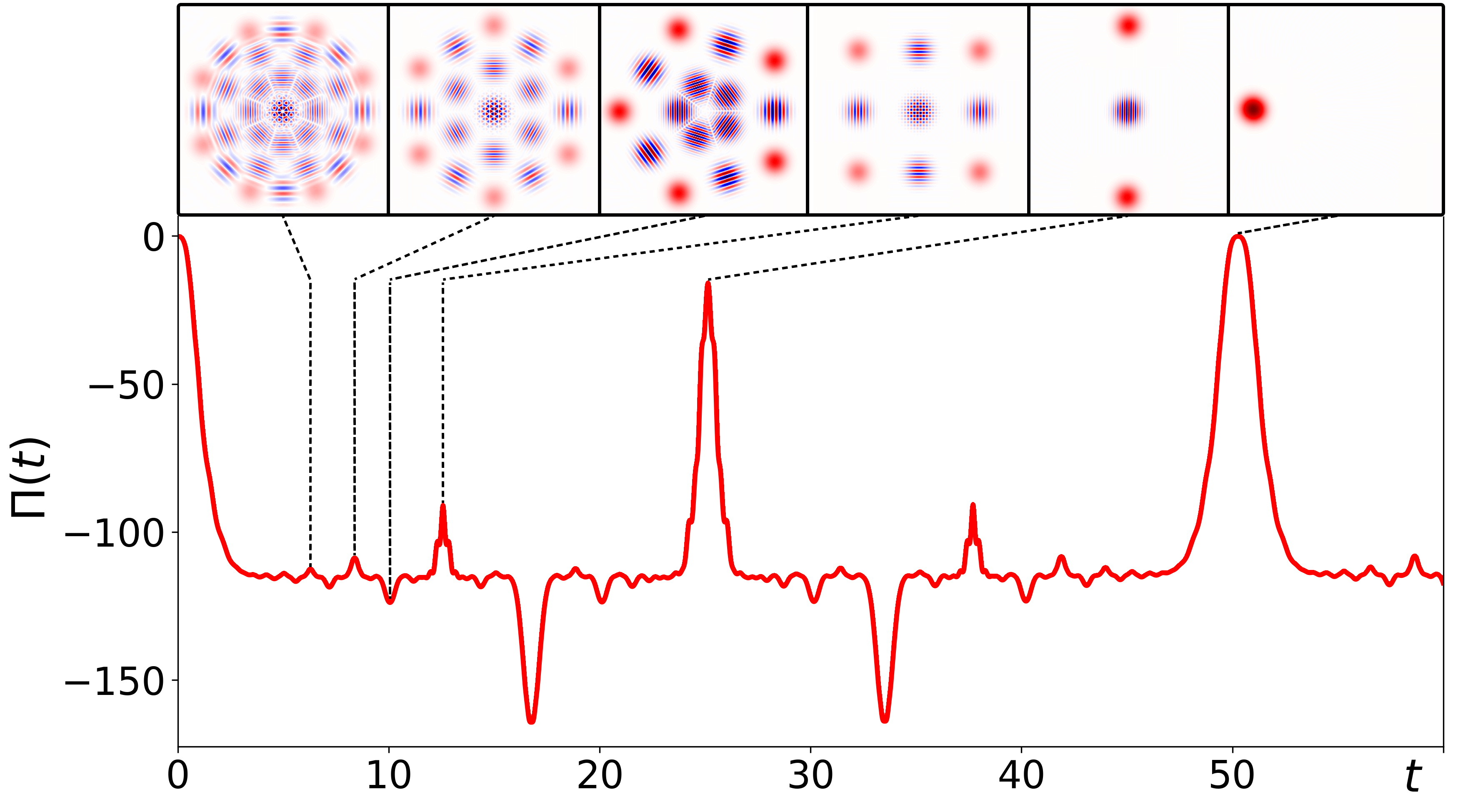
Figure 6: Smoothed $\Pi(t)$ picks out special states. Deviations of ${\Pi}(t)$ from the settled value ($\approx-115$) single out special states: the evolution shows recurrence of the initial state at time $T_{\Lambda_{+}}=16\pi\approx 50.3$ ($\Lambda_{+}=1/2$). Pronounced peaks and troughs at intermediate times identify fractional revival states Averbukh and Perelman (1989) with special $n$-fold symmetries.

We emphasize that the levelling-off behaviour of $\Pi(t)$ is in marked contrast to the classical case: for long enough times, in simple bound-state classical systems nonsingular states $\rho(t)$ get stretched out linearly Oliva and Steuernagel (2019) into ever finer threads [see Fig. 1(b)] therefore $\langle\!\!\,\langle\partial_{r}(-{\mathbf{\nabla}}\times{\mathbf{j}})\rangle\!\!\,\rangle\propto t$ Oliva and Steuernagel (2019). The quantum evolution counteracts this classical shear $s$ resulting in values of the shear suppression $\Pi$ which are opposite in sign to those of $s$ Oliva and Steuernagel (2019) (for the Kerr system sgn[$s$]=sgn[$\Lambda^{2}$]).

Moreover, starting from an initial Gaussian state, the magnitude $|\Pi(t)|$ initially grows the more the evolution stretches out the state into finer structures. Eventually quantum shear suppression stops classical shear from creating finer structures in phase space Oliva and Steuernagel (2019): $|\Pi(t)|$ levels off.

In other words, the quantum evolution is effectively “viscous”. This viscosity is the mechanism by which quantum evolution enforces that $W$ can typically not form structures below the size scale identified by Zurek Zurek (2001). Therefore, $\Pi(t)$ settles when the state has formed structures at the Zurek scale. This can, e.g., be quantified by monitoring the phase-spatial frequency content of $W$ as a function of time (for details see Ref.Oliva and Steuernagel (2019)).

Yet, quantum evolution is not truly viscous, it allows for revivals. Interestingly, these are picked up by the deviation of $\Pi(t)$ from the local time average. For the Kerr system, the special states for which this deviation is largest are (fractional) revival states Robinett (2004); Kirchmair et al. (2013) (see Fig. 6).

We emphasize that such revival states are traditionally picked up through the overlap of the evolved state with a suitably chosen reference state (such as a Gaussian initial state) Robinett (2004), instead, our measure $\Pi(t)$ does not depend on a reference state, this makes it more versatile than the use of wave-function overlaps.

We note that graphs of $\Pi(t)$ for anharmonic systems that do not have the symmetry of the Kerr system carry high frequency oscillations Oliva and Steuernagel (2019), whereas, due to the symmetry of the Kerr system, such oscillations are absent here. Generally, for other anharmonic systems without circular symmetry, graphs of as smooth as those for $\Pi(t)$ obtained in Fig. 6 require frequency filtering Oliva and Steuernagel (2019). In addition to the symmetries identified above, also in this regard are Kerr oscillators the simplest possible continuous quantum systems that alter quantum coherences.

To conclude, quantum dynamics that generates coherences in continuous systems is most easily studied in phase space and using Kerr systems, since these have special symmetries. The two symmetries we have identified are circular phase-space current ${\mathbf{J}}$, Eq. (7), and probability conservation for $W$ on rings, Eq. (14). These imply the absence of high-frequency components in $\Pi(t)$ of Eq. (18), see Fig. 6. We also have identified a quantum speedup of the propagation of wave-function pulses in phase space and we demonstrate that the dynamics of the Kerr system is “effectively viscous”. This can be quantified, explains the emergence of Zurek’s scale for the formation of minimum structures in quantum phase space, and can be used to pick out special quantum states.

The geometric nature of our approach helps us to guide the understanding of the generation of coherences in quantum dynamics and the formation of negativities of $W$ and will hopefully help pave the way to devise new strategies to protect coherences (for related ideas see Ref. Friedman and Blencowe (2017)).

VI Appendix

The Hamiltonian of anharmonic single-mode oscillators of the Kerr type has the form (4)

$${H}_{\Lambda}=\left(\frac{p^{2}}{2M}+\frac{k}{2}x^{2}\right)+\left(\Lambda\frac{p^{2}}{2M}+\lambda\frac{k}{2}x^{2}\right)^{2},$$ (19)

with $\Lambda=\lambda$. Here we keep the two parameters $\Lambda$ and $\lambda$ distinct to allow us to tune the system’s nonlinearities independently and help with keeping track of terms in the derivation of the form of ${\mathbf{J}}$.

The Wigner distribution of the Kerr oscillator obeys the phase-space continuity equation (3) Stobińska et al. (2008); Man’ko et al. (2010); Kelly et al. (2012)

$$\partial_{t}W(x,p,t) = \{\{H,W\}\}\ =\frac{2}{\hbar}~{}H(x,p)\ \sin\left({{\tfrac{\hbar}{2}}(\stackrel{{\scriptstyle\leftarrow}}{{\partial}}_{x}\stackrel{{\scriptstyle\rightarrow}}{{\partial}}_{p}-\stackrel{{\scriptstyle\leftarrow}}{{\partial}}_{p}\stackrel{{\scriptstyle\rightarrow}}{{\partial}}_{x})}\right)\ W(x,p,t)$$ (21)

$$= \left(\left[-\Lambda^{2}\frac{\hbar^{2}}{4M^{2}}p\partial_{x}^{3}+\lambda^{2}\frac{\hbar^{2}k^{2}}{4}x\partial_{p}^{3}-\left\{\Lambda\lambda{\frac{kx{p}^{2}}{M}}+\lambda^{2}{k}^{2}{x}^{3}\right\}\partial_{p}\right.\right.$$

$$\left.\left.-\Lambda\lambda\frac{\hbar^{2}k}{4M}p\partial_{x}\partial_{p}^{2}+\Lambda\lambda\frac{\hbar^{2}k}{4}x\partial_{p}\partial_{x}^{2}+\left\{\Lambda^{2}{\frac{{p}^{3}}{{M}^{2}}}+\Lambda\lambda{\frac{k{x}^{2}p}{M}}\right\}\partial_{x}\right]+\frac{p}{M}\partial_{x}-kx\partial_{p}\right)W(x,p,t).$$

The square brackets enclose the terms arising from the Kerr Hamiltonian’s anharmonic part, whereas the terms $\frac{p}{M}\partial_{x}-kx\partial_{p}$ stem from the harmonic oscillator contribution $p^{2}/(2M)+kx^{2}/2$.

The associated Wigner current components (6) are

$$J_{x} = \left[\hbar^{2}\left(-{\Lambda^{2}\frac{1}{4{M}^{2}}}p\partial_{x}^{2}-\Lambda\lambda{\frac{k}{4M}}p\partial_{p}^{2}\right)+\left\{{\Lambda^{2}\frac{{p}^{3}}{{M}^{2}}}+\Lambda\lambda{\frac{k{x}^{2}p}{M}}+{\frac{p}{M}}\right\}\right]W(x,p,t)$$ (22)

$$\mbox{and }J_{p} = \left[\hbar^{2}\left(\lambda^{2}\frac{k^{2}}{4}x\partial_{p}^{2}+\Lambda\lambda\frac{k}{4M}x\partial_{x}^{2}\right)-\left\{\lambda^{2}{k}^{2}{x}^{3}+\Lambda\lambda{\frac{kx{p}^{2}}{M}}+kx\right\}\right]W(x,p,t).$$ (23)

The curly brackets in Eqs. (22) and (23) contain the classical Hamiltonian current terms, and the round brackets contain the quantum terms.

To justify this assignment, note that the first term in $J_{p}$ is of the form $\frac{\hbar^{2}}{4\cdot 3!}\partial_{x}^{3}V\partial_{p}^{2}W$ Wigner (1932); Steuernagel et al. (2013) and thus has to be assigned to $J_{p}$, while the first term of $J_{x}$ is its “partner” term for the position case. What remains somewhat ambiguous is whether the second terms in (22) and (23) have been assigned correctly. To highlight this ambiguity consider

$$J_{x}^{(\sigma)} = J_{x}+\sigma\Lambda\lambda\frac{\hbar^{2}k}{4M}\left[x\partial_{p}\partial_{x}+p\partial_{p}^{2}\right]W(x,p,t)$$ (24)

$$\mbox{and }J_{p}^{(\sigma)} = J_{p}-\sigma\Lambda\lambda\frac{\hbar^{2}k}{4M}\left[x\partial_{x}^{2}+p\partial_{x}\partial_{p}\right]W(x,p,t),$$ (25)

parametrized by the interpolation parameter $\sigma$ with $0\leq\sigma\leq 1$. This interpolation fulfils the continuity equation (6) since the $\sigma$-dependent terms are divergence-free for  $0\leq\sigma\leq 1$.

To remove the ambiguity we can use Wigner current plots. We notice that the field plots of ${\mathbf{J}}^{(\sigma\neq 0)}$ do not “make sense” [see Fig. 7: ${\mathbf{J}}^{(\sigma=0)}$ of Eqs. (22) and (23), or Eq. (7) is the correct Wigner current expression].

We emphasize that this circular symmetry of ${\mathbf{J}}$, derived for $W$ formed from a superposition of two states, carries over to the case of general $W$ since any $W$ can be decomposed into sums of two-state superpositions.

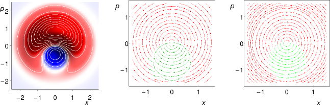
Figure 7: Wigner distribution, incorrect and correct Wigner current patterns for state $(|0\rangle+|1\rangle)/\sqrt{2}$. With $\Lambda=\lambda$ the dynamics of this superposition state is isomorphic to that of the harmonic oscillator, except for an extra phase due to the Kerr oscillator’s different energy spectrum. The incorrect expression ${\mathbf{J}}^{(\sigma=1)}$ for the current (middle panel) does not respect this isomorphism; it breaks the system’s circular symmetry and is therefore discarded. The correct expression ${\mathbf{J}}^{(\sigma=0)}$ for the current is depicted in the right-hand panel. The region represented by green is that where $W<0$; this leads to current inversion Steuernagel et al. (2013). For the Kerr system the only point of stagnation Steuernagel et al. (2013) of the current is the coordinate origin. When the current stagnates elsewhere in phase space, it forms lines of stagnation Kakofengitis and Steuernagel (2017).

References

- Kakofengitis et al. (2017) Dimitris Kakofengitis, Maxime Oliva, and Ole Steuernagel, “Wigner’s representation of quantum mechanics in integral form and its applications,” Phys. Rev. A 95, 022127 (2017), 1611.06891 .
- Oliva et al. (2017) Maxime Oliva, Dimitris Kakofengitis, and Ole Steuernagel, “Anharmonic quantum mechanical systems do not feature phase space trajectories,” Physica A 502, 201–210 (2017), 1611.03303 .
- Oliva and Steuernagel (2019) Maxime Oliva and Ole Steuernagel, “Dynamic shear suppression in quantum phase space,” Phys. Rev. Lett. 122, 020401 (2019), 1708.00398 .
- Wigner (1932) E. Wigner, “On the Quantum Correction For Thermodynamic Equilibrium,” Phys. Rev. 40, 749–759 (1932).
- Hillery et al. (1984) M. Hillery, R. F. O’Connell, M. O. Scully, and E. P. Wigner, “Distribution functions in physics: Fundamentals,” Phys. Rep. 106, 121 – 167 (1984).
- Zurek (2001) W. H. Zurek, “Sub-Planck structure in phase space and its relevance for quantum decoherence,” Nature 412, 712–717 (2001), quant-ph/0201118 .
- Leibfried et al. (1998) Dietrich Leibfried, Tilman Pfau, and Christopher Monroe, “Shadows and mirrors: reconstructing quantum states of atom motion,” Physics Today 51, 22–29 (1998).
- Tilma et al. (2016) Todd Tilma, Mark J. Everitt, John H. Samson, William J. Munro, and Kae Nemoto, “Wigner Functions for Arbitrary Quantum Systems,” Phys. Rev. Lett. 117, 180401 (2016).
- Heller (1976) Eric J. Heller, “”Wigner phase space method: Analysis for semiclassical applications”,” J. Chem. Phys. 65, 1289–1298 (1976).
- Feynman (1987) Richard P Feynman, Negative probability (Routledge London and New York, 1987) pp. 235–248.
- Berry and Balazs (1979) M. V. Berry and N. L. Balazs, “Evolution of semiclassical quantum states in phase space,” J. Phys. A 12, 625 (1979).
- Steuernagel et al. (2013) Ole Steuernagel, Dimitris Kakofengitis, and Georg Ritter, “Wigner flow reveals topological order in quantum phase space dynamics,” Phys. Rev. Lett. 110, 030401 (2013), 1208.2970 .
- Kakofengitis and Steuernagel (2017) Dimitris Kakofengitis and Ole Steuernagel, “Wigner’s quantum phase space flow in weakly-anharmonic weakly-excited two-state systems,” Eur. Phys. J. Plus 132, 381 (2017), 1411.3511 .
- Zachos et al. (2005) C. K. Zachos, D. B. Fairlie, and T. L. Curtright, Quantum Mechanics in Phase Space (World Scientific; Singapore, 2005).
- Moyal (1949) J. E. Moyal, “Quantum mechanics as a statistical theory,” Proc. Cambridge Philos. Soc. 45, 99 (1949).
- Walls and Milburn (1994) D. F. Walls and G. J. Milburn, Quantum Optics (Springer, 1994).
- Osborn and Marzlin (2009) T. A. Osborn and K.-P. Marzlin, “Moyal phase-space analysis of nonlinear optical kerr media,” J. Phys. A 42, 415302 (2009), 0905.3530 .
- Man’ko et al. (2010) V. I. Man’ko, G. Marmo, and F. Zaccaria, “Moyal and tomographic probability representations for f-oscillator quantum states,” Phys. Scr. 81, 045004 (2010), 0912.3424 .
- Kirchmair et al. (2013) G. Kirchmair, B. Vlastakis, Z. Leghtas, S. E. Nigg, H. Paik, E. Ginossar, M. Mirrahimi, L. Frunzio, S. M. Girvin, and R. J. Schoelkopf, “Observation of quantum state collapse and revival due to the single-photon Kerr effect,” Nature (London) 495, 205–209 (2013), 1211.2228 .
- Donoso and Martens (2001) A. Donoso and C. C. Martens, “Quantum tunneling using entangled classical trajectories,” Phys. Rev. Lett. 87, 223202 (2001).
- Bauke and Itzhak (2011) H. Bauke and N. R. Itzhak, “Visualizing quantum mechanics in phase space,” (2011), 1101.2683 .
- Nolte (2010) David D. Nolte, “The tangled tale of phase space,” Phys. Today 63, 33–38 (2010).
- Trahan and Wyatt (2003) C. J. Trahan and R. E. Wyatt, “Evolution of classical and quantum phase-space distributions: A new trajectory approach for phase space hydrodynamics,” J. Chem. Phys. 119, 7017–7029 (2003).
- Daligault (2003) J. Daligault, “Non-Hamiltonian dynamics and trajectory methods in quantum phase spaces,” Phys. Rev. A 68, 010501 (2003).
- Hudson (1974) R. L. Hudson, “When is the wigner quasi-probability density non-negative?” Rep. Math. Phys. 6, 249 – 252 (1974).
- Friedman and Blencowe (2017) O. D. Friedman and M. P. Blencowe, “The wigner flow for open quantum systems,” (2017), 1703.04844 .
- Averbukh and Perelman (1989) I. S. Averbukh and N. F. Perelman, “Fractional revivals: Universality in the long-term evolution of quantum wave packets beyond the correspondence principle dynamics,” Phys. Lett. A 139, 449–453 (1989).
- Robinett (2004) R. W. Robinett, “Quantum wave packet revivals,” Phys. Rep. 392, 1–119 (2004).
- Stobińska et al. (2008) M. Stobińska, G. J. Milburn, and K. Wódkiewicz, “Wigner function evolution of quantum states in the presence of self-Kerr interaction,” Phys. Rev. A 78, 013810 (2008), 0605166 .
- Kelly et al. (2012) A. Kelly, R. van Zon, J. Schofield, and R. Kapral, “Mapping quantum-classical liouville equation: Projectors and trajectories,” J. Chem. Phys. 136, 084101 (2012), 1201.1042 .