11institutetext: School of Data Science, Department of Statistics and finance
University of Science and Technology of China, Hefei, 230026, P.R.China
\tocauthor

Authors’ Instructions

THORS: An Efficient Approach for Making Classifiers Cost-sensitive

Ye Tian   Weiping Zhang Corresponding author. Email: zwp@ustc.edu.cn.
Abstract

In this paper, we propose an effective THresholding method based on ORder Statistic, called THORS, to convert an arbitrary scoring-type classifier, which can induce a continuous cumulative distribution function of the score, into a cost-sensitive one. The procedure, uses order statistic to find an optimal threshold for classification, requiring almost no knowledge of classifiers itself. Unlike common data-driven methods, we analytically show that THORS has theoretical guaranteed performance, theoretical bounds for the costs and lower time complexity. Coupled with empirical results on several real-world data sets, we argue that THORS is the preferred cost-sensitive technique.

Keywords:
Classification; Cost-sensitive learning; Imbalanced data set; Statistical learning; Threshold adjusting.

1 Introduction

Classification is one of the most important tasks in machine learning and data mining. A classifier is usually trained from a set of training instances with discrete and finite class labels to predict the class labels of new instances. Many effective classification algorithms have been developed, such as linear algorithms (Balakrishnama and Ganapathiraju,, 1998), neural network (Krizhevsky et al.,, 2012), Bayesian classifier (McCallum et al.,, 1998), decision tree (Safavian and Landgrebe,, 1991) and instance-based classifiers (Sheng and Ling,, 2009). However, most of the currently-available algorithms implicitly assume that all errors are equally costly, which may be inadequate for problems with various misclassification costs (Domingos,, 1999). In many KDD applications, costs are often different for different types of errors. For example, in fraud detection, undetected frauds with high transaction amounts are obviously more costly (Fan et al.,, 1999; Zonneveldt et al.,, 2010). Besides, in medical diagnosis, it’s far more serious to diagnose someone with a life-threatening disease as healthy than diagnose someone healthy as ill (Tong et al.,, 2018; Viaene and Dedene,, 2005). As a result, a lot of work related to cost-sensitive learning has been done recently and they seek to minimize total misclassification costs rather than error rate. Sheng and Ling, (2009) divide the existing cost-sensitive algorithms into two categories: One is to design cost-sensitive classifiers that are cost-sensitive in themselves (Chai et al.,, 2004; Drummond and Holte,, 2000; Turney,, 1994) and the other is to design a “wrapper” that converts any existing cost-insensitive classifiers into cost-sensitive ones, called cost-sensitive meta-learning or wrapper method (Domingos,, 1999; Elkan,, 2001; Fan et al.,, 1999; Sheng and Ling,, 2006; Sun et al.,, 2007; Ting,, 1998; Witten et al.,, 2016; Zadrozny and Elkan,, 2001; Zhao,, 2008). Our work belongs to the second category.

The wrapper method can be further categorized as thresholding, sampling and weighting (Sheng and Ling,, 2006). Thresholding finds the best probability (or other scores) which minimizes the total misclassification cost from the training instances as the threshold, and uses it to predict the class label of test instances. Metacost (Domingos,, 1999) is a thresholding method. It firstly learns a classifier on each multiple bootstrap replicates of the training set to obtain reliable probability estimations of training instances by voting, and then relabels training instances according to their estimated minimal cost classes, finally uses the relabeled training instances to build a cost-sensitive classifier. Metacost can be applied to multi-class problems and to arbitrary cost matrices. Instead of relabeling the training instances, Cost Sensitive Classifier (CSC) (Witten et al.,, 2016) relabels the test instances. Elkan, (2001) obtains the theoretical threshold for making optimal cost-sensitive classification in two-class case, and argues that changing the balance of negative and positive training instances has little effect on the classifier learned by standard decision tree learning methods (Elkan,, 2001). Noting that estimating the probability accurately is crucial in thresholding-based meta-learning methods, Zadrozny and Elkan, (2001) propose several methods to improve the calibration of probability estimates, while Sheng and Ling, (2006) develop an empirical thresholding method which does not require accurate estimation of probabilities Sheng and Ling, (2006). Alternatively, sampling method modifies the class distribution of the training data, then applies cost-insensitive classifiers on the sampled data directly. Weighting (Ting,, 1998) can be viewed as a sampling method, in which different types of instances in the training data are weighted according to the misclassification costs during classifier learning, such that the classifier strives to make fewer errors of the more costly type, resulting in lower overall cost. Methods based on weighting include Sun et al., (2007); Zadrozny et al., (2003); Zhao, (2008).

While a plethora of cost-sensitive methods have been investigated, several issues still remain to be addressed. Firstly, empirical comparisons instead of theoretical properties are frequently reported for the existing algorithms. The theoretical error bounds for the costs are less explored for most cost-sensitive classifiers. While common practices that directly limit the empirical false negative rate to no more than specified level show that the resulting classifiers are likely to have a much larger false negative rate. Secondly, the time complexity of a cost-sensitive classifier is an important concern since existing re-sampling and weighting methods are computationally more involved. We propose a THresholding method based on ORder Statistic method, named THORS, to convert an arbitrary scoring-type classifier, which induces a continuous cumulative distribution function of scores, into a cost-sensitive one. It uses the order statistics of classification scores on validation set to build an optimal classification threshold, instead of estimating the optimal threshold probability. We analytically show that the existence of the optimal threshold and the error bounds of costs because it does not need to re-sample the training instances. THORS also has lower time complexity compared with the existing popular cost-sensitive classifiers. It usually leads to smaller total cost than empirical approaches, Metacost, and Cost-proportionate Rejection Sampling (CRS) methods, even on the heavily imbalanced dataset.

The remainder of the paper is organized as follows. In Section 2 and 3, detailed THORS algorithm and its theoretical properties are described. In Section 4, we evaluate our method on three real data sets against other existing methods, such as theoretical thresholding, empirical thresholding, and meta-learning algorithms including Metacost and CRS. We conclude this paper by summarizing the main findings and outlining future research in Section 5.

2 The THORS Algorithm

The theory of cost-sensitive learning presented by (Elkan,, 2001; Sheng and Ling,, 2009) describes how the misclassification cost plays its role in various related cost-sensitive algorithms. Without loss of generality, we assume binary classification (i.e., positive and negative class) in this paper, where the objective is to predict the value of a binary-dependent variable, referred to as the class, based on a vector of independent variables (also called attributes or features). In THORS, the full data is divided into training set and validation set, which are used to train the classifier and find optimal threshold, respectively. Then the scoring function f𝑓f is trained using the training set and assigns a classification score to an observation x𝑥x, the class label is predicted by whether its score f(x)𝑓𝑥f(x) is larger than a threshold c𝑐c. Most popular classification methods are of this type, including SVMs, Naïve Bayes, logistic regression and neural networks. The classification scores can be strict probabilities or uncalibrated numeric values as long as a higher score indicates a higher probability of an observation belonging to the positive class. The optimal threshold c𝑐c is selected as the minimizer of estimated misclassification expected cost in (2) on validation set, which usually uses cross-validation to search the best threshold value from the training dataset.

2.1 Cost Matrix

In cost-sensitive learning, the costs of false positive (actual negative but predicted as positive; denoted as FP), false negative (FN), true positive (TP) and true negative (TN) can be given in a cost matrix, as shown in Table 1, where C(j,k)𝐶𝑗𝑘C(j,k) denotes the cost of classifying the instance be class k𝑘k when it is actually in class j𝑗j (j,k=0,1formulae-sequence𝑗𝑘01j,k=0,1). C(j,j)𝐶𝑗𝑗C(j,j) (TP and TN) is usually regarded as the “benefit”(i.e., negated cost) when the instance is predicted correctly.

Table 1: Cost Matrix of All the Instances in A Binary Classification
Actual Predict Negative Positive
Negative C(0,0)𝐶00C(0,0) C(0,1)𝐶01C(0,1)
Positive C(1,0)𝐶10C(1,0) C(1,1)𝐶11C(1,1)

Usually, the minority class is regarded as the positive class, and it is often more expensive to misclassify an actual positive instance into negative, than an actual negative instance into positive. That is, the value of FN or C(1,0)𝐶10C(1,0) is usually larger than that of FP or C(0,1)𝐶01C(0,1). This is true for the fraud detection example mentioned earlier (fraud transaction is usually rare, but predicting an actual fraud transaction as negative is usually more costly) and the medical diagnosis example. Without loss of generality, we consider the case where C(0,0)=C(1,1)=0𝐶00𝐶110C(0,0)=C(1,1)=0 and β=C(0,1)/C(1,0)𝛽𝐶01𝐶10\beta=C(0,1)/C(1,0) for some 0<β<10𝛽10<\beta<1. Under the case we consider, the expected cost for classifying n𝑛n instances is

C=i=1n[π0C(0,1)Pi(1|0)+π1C(1,0)Pi(0|1)],𝐶superscriptsubscript𝑖1𝑛delimited-[]subscript𝜋0𝐶01subscript𝑃𝑖conditional10subscript𝜋1𝐶10subscript𝑃𝑖conditional01C=\sum_{i=1}^{n}[\pi_{0}C(0,1)P_{i}(1|0)+\pi_{1}C(1,0)P_{i}(0|1)], (1)

where πjsubscript𝜋𝑗\pi_{j} is the marginal probability of class j𝑗j and Pi(1|0)subscript𝑃𝑖conditional10P_{i}(1|0) is the probability of classifying instance i𝑖i into class 1 when it actually in class 0, which is called the False Positive Rate (FPR); Pi(0|1)subscript𝑃𝑖conditional01P_{i}(0|1) is the probability of classifying instance i𝑖i into class 0 when it actually in class 1, and is called False Negative Rate (FNR). Obviously, the classification error is a weighted sum of FNR and FPR. In practice, both πjsubscript𝜋𝑗\pi_{j} and Pi(j|k)(j,k=0,1)P_{i}(j|k)(j,k=0,1) are unknown. They should be estimated on validation set and plugged into (1), where the corresponding estimations are π^jsubscript^𝜋𝑗\widehat{\pi}_{j} and P^i(j|k)subscript^𝑃𝑖conditional𝑗𝑘\widehat{P}_{i}(j|k) (j,k=0,1)formulae-sequence𝑗𝑘01(j,k=0,1) and we have the estimated expected cost

C^=i=1n[π^0C(0,1)P^i(1|0)+π^1C(1,0)P^i(0|1)].^𝐶superscriptsubscript𝑖1𝑛delimited-[]subscript^𝜋0𝐶01subscript^𝑃𝑖conditional10subscript^𝜋1𝐶10subscript^𝑃𝑖conditional01\widehat{C}=\sum_{i=1}^{n}[\widehat{\pi}_{0}C(0,1)\widehat{P}_{i}(1|0)+\widehat{\pi}_{1}C(1,0)\widehat{P}_{i}(0|1)]. (2)

2.2 Thresholding on Order Statistic

Firstly we split the full data into training set and validation set. The training set will be used for training the classifier and the validation set will help us to find the optimal threshold. Intuitively, the optimal threshold splits the classification scores into two parts and produces minimal estimated expected misclassification cost in (2) on the validation set. Our proposed THORS algorithm picks one of the scores as the optimal threshold which is an order statistic of scores to obtain a minimal total misclassification cost on validation set. Recently, Tong et al., (2018) show that a binary classifier by choosing order statistic as an optimal threshold guarantees the desired high-probability control of type I error Pi(1|0)subscript𝑃𝑖conditional10P_{i}(1|0). We prove that the errors and total misclassification cost by THORS algorithm are similarly bounded theoretically.

For a given binary classifier f𝑓f, a new instance i𝑖i with the predictor vector xisubscript𝑥𝑖x_{i} is predicted as class positive (1) if f(xi)>c𝑓subscript𝑥𝑖superscript𝑐f(x_{i})>c^{*}, otherwise it will be classified into class negative (0), that is,

ψ(xi)={0,f(xi)c,1,f(xi)>c.𝜓subscript𝑥𝑖cases0missing-subexpression𝑓subscript𝑥𝑖superscript𝑐1missing-subexpression𝑓subscript𝑥𝑖superscript𝑐\psi(x_{i})=\left\{\begin{array}[]{rcl}0,&&f(x_{i})\leq c^{*},\\ 1,&&f(x_{i})>c^{*}.\\ \end{array}\right. (3)

where csuperscript𝑐c^{*} is the optimal threshold needing to be learned from the validation set. The score function f𝑓f is learned from the training data set. f(xi)𝑓subscript𝑥𝑖f(x_{i}) is the score of instance i𝑖i with feature vector xisubscript𝑥𝑖x_{i} under the classifier ψ𝜓\psi. Applying the classifier f𝑓f to the validation set of size nvsubscript𝑛𝑣n_{v} with n0subscript𝑛0n_{0} class 0 and n1subscript𝑛1n_{1} class 1 instances, we obtain nvsubscript𝑛𝑣n_{v} sorted scores as T(1)T(2)T(nv)subscript𝑇1subscript𝑇2subscript𝑇subscript𝑛𝑣T_{(1)}\leq T_{(2)}\leq...\leq T_{(n_{v})}, and scores in class 0 and class 1 are denoted as T(1)0T(2)0T(n0)0subscriptsuperscript𝑇01subscriptsuperscript𝑇02subscriptsuperscript𝑇0subscript𝑛0T^{0}_{(1)}\leq T^{0}_{(2)}\leq...\leq T^{0}_{(n_{0})} and T(1)1T(2)1T(n1)1subscriptsuperscript𝑇11subscriptsuperscript𝑇12subscriptsuperscript𝑇1subscript𝑛1T^{1}_{(1)}\leq T^{1}_{(2)}\leq...\leq T^{1}_{(n_{1})}, respectively. Then we have the following theorem for selecting the optimal threshold.

Theorem 2.1.

Let k0=argmax{1in0:T(i)0T(k)}subscript𝑘0:1𝑖subscript𝑛0subscriptsuperscript𝑇0𝑖subscript𝑇𝑘k_{0}=\arg\max\{1\leq i\leq n_{0}:T^{0}_{(i)}\leq T_{(k)}\} and k1=argmax{1in1:T(i)1T(k)}subscript𝑘1:1𝑖subscript𝑛1subscriptsuperscript𝑇1𝑖subscript𝑇𝑘k_{1}=\arg\max\{1\leq i\leq n_{1}:T^{1}_{(i)}\leq T_{(k)}\}. π^0=n0nvsubscript^𝜋0subscript𝑛0subscript𝑛𝑣\widehat{\pi}_{0}=\frac{n_{0}}{n_{v}} and π^1=n1nvsubscript^𝜋1subscript𝑛1subscript𝑛𝑣\widehat{\pi}_{1}=\frac{n_{1}}{n_{v}} are estimations of the marginal probability of class 0 and 1 samples in the population. Then the optimal threshold can be decided by minimizing the following part of estimated expected cost (2) on validation set,

π^1k1n1βπ^0k0n0.subscript^𝜋1subscript𝑘1subscript𝑛1𝛽subscript^𝜋0subscript𝑘0subscript𝑛0\frac{\widehat{\pi}_{1}k_{1}}{n_{1}}-\frac{\beta\widehat{\pi}_{0}k_{0}}{n_{0}}. (4)

That is, the optimal threshold c=T(k)superscript𝑐subscript𝑇superscript𝑘c^{*}=T_{(k^{*})}, where

k=argmin1knv{π^1k1n1βπ^0k0n0}.superscript𝑘subscript1𝑘subscript𝑛𝑣subscript^𝜋1subscript𝑘1subscript𝑛1𝛽subscript^𝜋0subscript𝑘0subscript𝑛0k^{*}=\arg\min\limits_{1\leq k\leq n_{v}}\Big{\{}\frac{\widehat{\pi}_{1}k_{1}}{n_{1}}-\frac{\beta\widehat{\pi}_{0}k_{0}}{n_{0}}\Big{\}}. (5)

It is worth noting that Theorem 2.1 does not rely on any distributional assumptions or on base algorithm characteristics. Besides, from Theorem 2.1 it is known that if the rank k𝑘k is fixed then k0subscript𝑘0k_{0} and k1subscript𝑘1k_{1} become fixed as well. Therefore we can estimate (4) for each choice of k𝑘k on validation set and choose the optimal one to make (5) minimal in nearly linear time, which is much more efficient than most of the empirical methods.

We summarize the THORS method as the following Algorithm 1.

Algorithm 1 THORS algorithm

Input:
      Dvsubscript𝐷𝑣D_{v}: Validation set with size nvsubscript𝑛𝑣n_{v}, including n0subscript𝑛0n_{0} class 0 and n1subscript𝑛1n_{1} class 1 samples
      f𝑓f: Classification score function
Output:
      csuperscript𝑐c^{*}: Estimated optimal threshold
Other parameters:
      π^0subscript^𝜋0\widehat{\pi}_{0}: n0nvsubscript𝑛0subscript𝑛𝑣\frac{n_{0}}{n_{v}}
      π^1subscript^𝜋1\widehat{\pi}_{1}: n1nvsubscript𝑛1subscript𝑛𝑣\frac{n_{1}}{n_{v}}
      xisubscript𝑥𝑖x_{i}: Feature vector of instance i𝑖i
      x(i)subscript𝑥𝑖x_{(i)}: Feature vector of i𝑖i-th order statistic
      Y(i)subscript𝑌𝑖Y_{(i)}: True class of i𝑖i-th order statistic

1:  T1,,Tnvf(x1),,f(xnv)formulae-sequencesubscript𝑇1subscript𝑇subscript𝑛𝑣𝑓subscript𝑥1𝑓subscript𝑥subscript𝑛𝑣T_{1},...,T_{n_{v}}\longleftarrow f(x_{1}),...,f(x_{n_{v}})
2:  T(1),,T(nv)subscript𝑇1subscript𝑇subscript𝑛𝑣T_{(1)},...,T_{(n_{v})} \longleftarrow sort T1,,Tnvsubscript𝑇1subscript𝑇subscript𝑛𝑣T_{1},...,T_{n_{v}}
3:  l0,l10subscript𝑙0subscript𝑙10l_{0},l_{1}\longleftarrow 0
4:  for k𝑘k in {1,2,,nv}12subscript𝑛𝑣\{1,2,...,n_{v}\} do
5:     if Y(k)=0subscript𝑌𝑘0Y_{(k)}=0 then
6:        l0l0+1subscript𝑙0subscript𝑙01l_{0}\longleftarrow l_{0}+1
7:     else
8:        l1l1+1subscript𝑙1subscript𝑙11l_{1}\longleftarrow l_{1}+1
9:     end if
10:     k0l0,k1l1formulae-sequencesubscript𝑘0subscript𝑙0subscript𝑘1subscript𝑙1k_{0}\longleftarrow l_{0},k_{1}\longleftarrow l_{1}
11:     C(k)π^1k1n1βπ^0k0n0𝐶𝑘subscript^𝜋1subscript𝑘1subscript𝑛1𝛽subscript^𝜋0subscript𝑘0subscript𝑛0C(k)\longleftarrow\frac{\widehat{\pi}_{1}k_{1}}{n_{1}}-\frac{\beta\widehat{\pi}_{0}k_{0}}{n_{0}}
12:  end for
13:  kargminkC(k)superscript𝑘subscript𝑎𝑟𝑔𝑚𝑖𝑛𝑘𝐶𝑘k^{*}\longleftarrow\mathop{argmin}\limits_{k}C(k)
14:  threshold cT(k)superscript𝑐subscript𝑇superscript𝑘c^{*}\longleftarrow T_{(k^{*})}
15:  return  csuperscript𝑐c^{*}

3 Properties

For the THORS method described in the previous section, we can show that its FPR, FNR and expected misclassification cost are bounded by the following theorems. These properties hold for any score-type classifier that introduces a continuous cumulative distribution function of the score. For discontinuous cases, properties can be approximately correct.

3.1 Theoretical Upper Bound

Under Algorithm 1, let Ti=f(xi)subscript𝑇𝑖𝑓subscript𝑥𝑖T_{i}=f(x_{i}) be the score for a new instance i𝑖i with class label cisubscript𝑐𝑖c_{i} and feature xisubscript𝑥𝑖x_{i} under the classifier ψ(xi)𝜓subscript𝑥𝑖\psi(x_{i}), the corresponding FNR and FPR are αi1=P(ψ(xi)=0|ci=1)subscript𝛼𝑖1𝑃𝜓subscript𝑥𝑖conditional0subscript𝑐𝑖1\alpha_{i1}=P(\psi(x_{i})=0|c_{i}=1) and αi0=P(ψ(xi)=1|ci=0)subscript𝛼𝑖0𝑃𝜓subscript𝑥𝑖conditional1subscript𝑐𝑖0\alpha_{i0}=P(\psi(x_{i})=1|c_{i}=0), respectively. Due to the randomness of the order statistic and the relationship between order statistic of scores and the threshold we choose, here both two types of error rates are random variables. Noting that c=T(k)superscript𝑐subscript𝑇superscript𝑘c^{*}=T_{(k^{*})} is fixed in the computation of conditional probabilities, for the bounds of cumulative distribution functions of FNR and FPR, we have the following result.

Theorem 3.1.

Let αi1subscript𝛼𝑖1\alpha_{i1} and αi0subscript𝛼𝑖0\alpha_{i0} be FNR and FPR of classifying new instance i𝑖i with true class label cisubscript𝑐𝑖c_{i} using the classifier ψ(xi)𝜓subscript𝑥𝑖\psi(x_{i}) under THORS algorithm, respectively. When the distribution of the score is continuous, for any x(0,1)𝑥01x\in(0,1), we have

j=n0k0+1n0(n0j)xj(1x)n0jsuperscriptsubscript𝑗subscript𝑛0subscript𝑘01subscript𝑛0binomialsubscript𝑛0𝑗superscript𝑥𝑗superscript1𝑥subscript𝑛0𝑗absent\displaystyle\sum_{j=n_{0}-k_{0}+1}^{n_{0}}\binom{n_{0}}{j}x^{j}(1-x)^{n_{0}-j}\leq P(αi0x)j=n0k0n0(n0j)xj(1x)n0j,𝑃subscript𝛼𝑖0𝑥superscriptsubscript𝑗subscript𝑛0subscript𝑘0subscript𝑛0binomialsubscript𝑛0𝑗superscript𝑥𝑗superscript1𝑥subscript𝑛0𝑗\displaystyle P(\alpha_{i0}\leq x)\leq\sum_{j=n_{0}-k_{0}}^{n_{0}}\binom{n_{0}}{j}x^{j}(1-x)^{n_{0}-j}, (6)
j=k1+1n1(n1j)xj(1x)n1jsuperscriptsubscript𝑗subscript𝑘11subscript𝑛1binomialsubscript𝑛1𝑗superscript𝑥𝑗superscript1𝑥subscript𝑛1𝑗absent\displaystyle\sum_{j=k_{1}+1}^{n_{1}}\binom{n_{1}}{j}x^{j}(1-x)^{n_{1}-j}\leq P(αi1x)j=k1n1(n1j)xj(1x)n1j.𝑃subscript𝛼𝑖1𝑥superscriptsubscript𝑗subscript𝑘1subscript𝑛1binomialsubscript𝑛1𝑗superscript𝑥𝑗superscript1𝑥subscript𝑛1𝑗\displaystyle P(\alpha_{i1}\leq x)\leq\sum_{j=k_{1}}^{n_{1}}\binom{n_{1}}{j}x^{j}(1-x)^{n_{1}-j}. (7)

where the numbers of class 0 and 1 in validation set are denoted as n0subscript𝑛0n_{0} and n1subscript𝑛1n_{1} and definitions of k0subscript𝑘0k_{0}, k1subscript𝑘1k_{1} are the same as Theorem 2.1. That is, the bounds of cumulative distribution function of FNR and FPR are only dependent on ni,ki(i=0,1)subscript𝑛𝑖subscript𝑘𝑖𝑖01n_{i},k_{i}(i=0,1), which will be fixed for specified validation set.

According to Theorem 3.1, we have the following high probability upper bound for the expected cost on ntesubscript𝑛𝑡𝑒n_{te} new instances.

Theorem 3.2.

Let C𝐶C be the expected misclassification cost of the THORS algorithm on ntesubscript𝑛𝑡𝑒n_{te} new instances, then there exist some constant C,M,σsuperscript𝐶𝑀𝜎C^{*},M,\sigma such that

P(CC+tσ)1exp{t22+2M3σt},𝑃𝐶superscript𝐶𝑡𝜎1𝑒𝑥𝑝superscript𝑡222𝑀3𝜎𝑡P(C\leq C^{*}+t\sigma)\geq 1-exp\Bigg{\{}-\frac{t^{2}}{2+\frac{2M}{3\sigma}t}\Bigg{\}}, (8)

where C,Msuperscript𝐶𝑀C^{*},M and σ𝜎\sigma satisfy

Csuperscript𝐶\displaystyle C^{*} =nteC(1,0)[βπ0(n0k0+1n0+1)+π1(k1+1n1+1)],absentsubscript𝑛𝑡𝑒𝐶10delimited-[]𝛽subscript𝜋0subscript𝑛0subscript𝑘01subscript𝑛01subscript𝜋1subscript𝑘11subscript𝑛11\displaystyle=n_{te}C(1,0)\Big{[}\beta\pi_{0}\Big{(}\frac{n_{0}-k_{0}+1}{n_{0}+1}\Big{)}+\pi_{1}\Big{(}\frac{k_{1}+1}{n_{1}+1}\Big{)}\Big{]}, (9)
M𝑀\displaystyle M =max{π1C(1,0)max(k1+1n1+1,1k1+1n1+1),\displaystyle=max\Big{\{}\pi_{1}C(1,0)max\Big{(}\frac{k_{1}+1}{n_{1}+1},1-\frac{k_{1}+1}{n_{1}+1}\Big{)},
βπ0C(1,0)max(n0k0+1n0+1,1n0k0+1n0+1)},\displaystyle\qquad\beta\pi_{0}C(1,0)max\Big{(}\frac{n_{0}-k_{0}+1}{n_{0}+1},1-\frac{n_{0}-k_{0}+1}{n_{0}+1}\Big{)}\Big{\}}, (10)
σ2superscript𝜎2\displaystyle\sigma^{2} =nte[C(1,0)]2[π12(k1+1)(n1k1)(n1+1)2(n1+2)+(βπ0)2k0(n0k0+1)(n0+1)2(n0+2)].absentsubscript𝑛𝑡𝑒superscriptdelimited-[]𝐶102delimited-[]superscriptsubscript𝜋12subscript𝑘11subscript𝑛1subscript𝑘1superscriptsubscript𝑛112subscript𝑛12superscript𝛽subscript𝜋02subscript𝑘0subscript𝑛0subscript𝑘01superscriptsubscript𝑛012subscript𝑛02\displaystyle=n_{te}[C(1,0)]^{2}\Big{[}\pi_{1}^{2}\frac{(k_{1}+1)(n_{1}-k_{1})}{(n_{1}+1)^{2}(n_{1}+2)}+(\beta\pi_{0})^{2}\frac{k_{0}(n_{0}-k_{0}+1)}{(n_{0}+1)^{2}(n_{0}+2)}\Big{]}. (11)

Here ntesubscript𝑛𝑡𝑒n_{te} represents the number of new instances and n0,n1,k0,k1subscript𝑛0subscript𝑛1subscript𝑘0subscript𝑘1n_{0},n_{1},k_{0},k_{1} are defined the same as Theorem 3.1.

3.2 Time Complexity

For empirical method the time complexity is a3rangepcnvsubscript𝑎3𝑟𝑎𝑛𝑔𝑒𝑝𝑐subscript𝑛𝑣a_{3}\cdot\frac{range}{pc}\cdot n_{v}, where range is the searching range for optimal threshold and pc𝑝𝑐pc is the searching precision. And a3subscript𝑎3a_{3} is related to the type of classifier itself and nvsubscript𝑛𝑣n_{v} is the size of validation set used for estimate the threshold (Sheng and Ling,, 2006). And the time complexity of Metacost method (Domingos,, 1999) is a4mntrsubscript𝑎4𝑚subscript𝑛𝑡𝑟a_{4}\cdot m\cdot n_{tr} in which m𝑚m is the number of resampled instances to generate and ntrsubscript𝑛𝑡𝑟n_{tr} is the size of training set. a4subscript𝑎4a_{4} is the constant related to classifier and the sampling algorithm. For Cost-proportionate Rejection Sampling (CRS) (Witten et al.,, 2016) that is a5Zcntrsubscript𝑎5𝑍𝑐subscript𝑛𝑡𝑟a_{5}\cdot\frac{Z}{c}\cdot n_{tr}, where cZ𝑐𝑍\frac{c}{Z} is acceptance probability and both c𝑐c, Z𝑍Z are defined in (Witten et al.,, 2016). a5subscript𝑎5a_{5} is a constant related to the performance of classifier itself. To obtain a good performance, pc,m𝑝𝑐𝑚pc,m are needed to be chosen not so small, leading to high time-complexity. However, our numerical studies in the next section show that THORS can find the optimal threshold more faster than empirical method and Metacost in a short time. Although the time complexity of CRS is also small, the performance of it is much worse than THORS for real data, which will be shown by the following section.

Theorem 3.3.

The time-complexity of THORS algorithm is a1nvlognv+a2nvsubscript𝑎1subscript𝑛𝑣𝑙𝑜𝑔subscript𝑛𝑣subscript𝑎2subscript𝑛𝑣a_{1}n_{v}log\,n_{v}+a_{2}n_{v}, where a1subscript𝑎1a_{1}, a2subscript𝑎2a_{2} are constants related to the sorting method and the classifier itself respectively (a1subscript𝑎1a_{1} is very small). And nvsubscript𝑛𝑣n_{v} is the size of validation set.

3.3 Short Theoretical Bounds of Misclassification Cost Expectation

We will see that the range of expected misclassification cost will approximate to short bounds under a high probability when the validation set size nvsubscript𝑛𝑣n_{v} is large enough.

Theorem 3.4.

The expected misclassification cost C𝐶C is bounded by some constants, that is

P(C1CεCC2+Cε)𝑃subscript𝐶1subscript𝐶𝜀𝐶subscript𝐶2subscript𝐶𝜀\displaystyle P(C_{1}-C_{\varepsilon}\leq C\leq C_{2}+C_{\varepsilon})
1nte[exp{2[ε+n1k1n1(n1+1)]2n1}+exp{2[ε+k1n1(n1+1)]2n1}\displaystyle\geq 1-n_{te}\Big{[}exp\Big{\{}-2\Big{[}\varepsilon+\frac{n_{1}-k_{1}}{n_{1}(n_{1}+1)}\Big{]}^{2}n_{1}\Big{\}}+exp\Big{\{}-2\Big{[}\varepsilon+\frac{k_{1}}{n_{1}(n_{1}+1)}\Big{]}^{2}n_{1}\Big{\}}
+exp{2[ε+k0n0(n0+1)]2n0}+exp{2[ε+n0k0n0(n0+1)]2n0}]\displaystyle+exp\Big{\{}-2\Big{[}\varepsilon+\frac{k_{0}}{n_{0}(n_{0}+1)}\Big{]}^{2}n_{0}\Big{\}}+exp\Big{\{}-2\Big{[}\varepsilon+\frac{n_{0}-k_{0}}{n_{0}(n_{0}+1)}\Big{]}^{2}n_{0}\Big{\}}\Big{]}
1O(exp{ε2nv}).absent1𝑂𝑒𝑥𝑝superscript𝜀2subscript𝑛𝑣\displaystyle\geq 1-O(exp\{-\varepsilon^{2}n_{v}\}). (12)

Particularly, the cost C𝐶C is upper-bounded,

P(CC2+Cε)𝑃𝐶subscript𝐶2subscript𝐶𝜀\displaystyle P(C\leq C_{2}+C_{\varepsilon})
1nte[exp{2[ε+k1n1(n1+1)]2n1}+exp{2[ε+n0k0n0(n0+1)]2n0}]absent1subscript𝑛𝑡𝑒delimited-[]𝑒𝑥𝑝2superscriptdelimited-[]𝜀subscript𝑘1subscript𝑛1subscript𝑛112subscript𝑛1𝑒𝑥𝑝2superscriptdelimited-[]𝜀subscript𝑛0subscript𝑘0subscript𝑛0subscript𝑛012subscript𝑛0\displaystyle\geq 1-n_{te}\Big{[}exp\Big{\{}-2\Big{[}\varepsilon+\frac{k_{1}}{n_{1}(n_{1}+1)}\Big{]}^{2}n_{1}\Big{\}}+exp\Big{\{}-2\Big{[}\varepsilon+\frac{n_{0}-k_{0}}{n_{0}(n_{0}+1)}\Big{]}^{2}n_{0}\Big{\}}\Big{]} (13)
1O(exp{ε2nv}).absent1𝑂𝑒𝑥𝑝superscript𝜀2subscript𝑛𝑣\displaystyle\geq 1-O(exp\{-\varepsilon^{2}n_{v}\}). (14)

where

C1subscript𝐶1\displaystyle C_{1} =nteC(1,0)[π1(k1n1+1)+βπ0(n0k0n0+1)],absentsubscript𝑛𝑡𝑒𝐶10delimited-[]subscript𝜋1subscript𝑘1subscript𝑛11𝛽subscript𝜋0subscript𝑛0subscript𝑘0subscript𝑛01\displaystyle=n_{te}C(1,0)\Big{[}\pi_{1}\Big{(}\frac{k_{1}}{n_{1}+1}\Big{)}+\beta\pi_{0}\Big{(}\frac{n_{0}-k_{0}}{n_{0}+1}\Big{)}\Big{]}, (15)
C2subscript𝐶2\displaystyle C_{2} =nteC(1,0)[π1(k1+1n1+1)+βπ0(n0k0+1n0+1)],absentsubscript𝑛𝑡𝑒𝐶10delimited-[]subscript𝜋1subscript𝑘11subscript𝑛11𝛽subscript𝜋0subscript𝑛0subscript𝑘01subscript𝑛01\displaystyle=n_{te}C(1,0)\Big{[}\pi_{1}\Big{(}\frac{k_{1}+1}{n_{1}+1}\Big{)}+\beta\pi_{0}\Big{(}\frac{n_{0}-k_{0}+1}{n_{0}+1}\Big{)}\Big{]}, (16)
Cεsubscript𝐶𝜀\displaystyle C_{\varepsilon} =nteC(1,0)(π1+βπ0)ε,absentsubscript𝑛𝑡𝑒𝐶10subscript𝜋1𝛽subscript𝜋0𝜀\displaystyle=n_{te}C(1,0)(\pi_{1}+\beta\pi_{0})\varepsilon, (17)

where ntesubscript𝑛𝑡𝑒n_{te} is the size of test set.

When nvsubscript𝑛𝑣n_{v} is large enough, ε𝜀\varepsilon can be taken as a small number and then the length of the interval [C1Cε,C2+Cε]subscript𝐶1subscript𝐶𝜀subscript𝐶2subscript𝐶𝜀[C_{1}-C_{\varepsilon},C_{2}+C_{\varepsilon}] could be relatively small and the upper bound C2+Cεsubscript𝐶2subscript𝐶𝜀C_{2}+C_{\varepsilon} would approximate to the least upper bound.
Furthermore, the following theorem is useful for estimating the size of a validation set to control expected cost with given precision.

Theorem 3.5.

Let n0subscript𝑛0n_{0} and n1subscript𝑛1n_{1} be the size of class 0 and class 1 instances in validation set, g^nv(x)subscript^𝑔subscript𝑛𝑣𝑥\widehat{g}_{n_{v}}(x) and g(x)𝑔𝑥g(x) be empirical expected cost for each sample on validation set C^nv^𝐶subscript𝑛𝑣\frac{\widehat{C}}{n_{v}} and the expected cost for each sample in population when threshold is x𝑥x, respectively. Denote α^i0=1k0n0,α^i1=k1n1formulae-sequencesubscript^𝛼𝑖01subscript𝑘0subscript𝑛0subscript^𝛼𝑖1subscript𝑘1subscript𝑛1\widehat{\alpha}_{i0}=1-\frac{k_{0}}{n_{0}},\widehat{\alpha}_{i1}=\frac{k_{1}}{n_{1}} as the empirical FPR and FNR on validation set, and αi0,αi1subscript𝛼𝑖0subscript𝛼𝑖1\alpha_{i0},\alpha_{i1} as FPR and FNR in population, based on optimal threshold obtaining by THORS. If the following four assumptions hold:
(A1) g(x)𝑔𝑥g(x) is continuous;
(A2) g^nv(x)𝑝g(x)𝑝subscript^𝑔subscript𝑛𝑣𝑥𝑔𝑥\widehat{g}_{n_{v}}(x)\xrightarrow{p}g(x), uniformly for fixed x𝑥x, as nvsubscript𝑛𝑣n_{v}\longrightarrow\infty;
(A3) α^i0=n0k0n0𝑝αi0,α^i1=k1n1𝑝αi1formulae-sequencesubscript^𝛼𝑖0subscript𝑛0subscript𝑘0subscript𝑛0𝑝subscript𝛼𝑖0subscript^𝛼𝑖1subscript𝑘1subscript𝑛1𝑝subscript𝛼𝑖1\widehat{\alpha}_{i0}=\frac{n_{0}-k_{0}}{n_{0}}\xrightarrow{p}\alpha_{i0},\widehat{\alpha}_{i1}=\frac{k_{1}}{n_{1}}\xrightarrow{p}\alpha_{i1}, as nvsubscript𝑛𝑣n_{v}\longrightarrow\infty;
(A4) g(x)𝑔𝑥g(x) has a unique minimal point at which g𝑔g reaches its minimum,
where k0subscript𝑘0k_{0} and k1subscript𝑘1k_{1} are defined as Theorem 2.1, then there exist

n0k0n0+1subscript𝑛0subscript𝑘0subscript𝑛01\displaystyle\frac{n_{0}-k_{0}}{n_{0}+1} 𝑝constant,𝑝absent𝑐𝑜𝑛𝑠𝑡𝑎𝑛𝑡\displaystyle\xrightarrow{p}\,\,constant, (18)
k1n1+1subscript𝑘1subscript𝑛11\displaystyle\frac{k_{1}}{n_{1}+1} 𝑝constant,𝑝absent𝑐𝑜𝑛𝑠𝑡𝑎𝑛𝑡\displaystyle\xrightarrow{p}\,\,constant, (19)

as nvsubscript𝑛𝑣n_{v}\longrightarrow\infty.

It is easy to see that assumption (A1) will always hold for a scoring-type classifier. Besides, it’s natural to assume that the empirical cost or error rate on validation set converges to population cost or error rate in probability. Thus assumption (A2) and (A3) follow reasonably. The assumption (A4) is related to the problem itself, most well-defined problems satisfy such assumption. This assumption guarantees that our solution can be stable. For (18) and (19), the ratios k1n1+1subscript𝑘1subscript𝑛11\frac{k_{1}}{n_{1}+1} and n0k0n0+1subscript𝑛0subscript𝑘0subscript𝑛01\frac{n_{0}-k_{0}}{n_{0}+1} can be regarded as constant as nvsubscript𝑛𝑣n_{v} goes to infinity in practice if these assumptions hold. Then if Cεsubscript𝐶𝜀C_{\varepsilon} is given, then ε𝜀\varepsilon can be obtained. Let n1=π^1nvsubscript𝑛1subscript^𝜋1subscript𝑛𝑣n_{1}=\widehat{\pi}_{1}n_{v} and n0=π^0nvsubscript𝑛0subscript^𝜋0subscript𝑛𝑣n_{0}=\widehat{\pi}_{0}n_{v} approximately, nvsubscript𝑛𝑣n_{v} can be solved from (13) if we let (13) be a fixed number between 0 and 1. The size nvsubscript𝑛𝑣n_{v} is a conservative estimation of the minimal size to control the cost under a fixed probability. We will calculate this for specific datasets in the following section.

4 Case Studies

In this section, we will focus on three real datasets from UCI Machine Learning Repository, in which their imbalance rates decrease from 59:1 to 1.84:1. THORS will be applied on them and results will be compared with other thresholding and meta-learning methods, including both total cost on test set and average running time on the 8 GB RAM laptop with Intel® Core™  i5-6300U CPU. The results show that THORS outperforms the alternatives even when the data set is heavily imbalanced.

4.1 Scania Trucks Data

We implement THORS on a Scania trucks dataset of UCI Machine Learning Repository. It records 60,000 component failures for a specific component of the APS system. And these samples fall into two categories: 1,000 failures for a specific component of the APS system and 59,000 ones not related to APS. To formulate this problem into a cost-sensitive classification one, we denote APS related failures as class 1 (positive) and unrelated ones as class 0 (negative). In this case, FP refers to the cost that an unnecessary check needs to be done by a mechanic at a workshop, while FN refers to the cost of missing a faulty truck, which may cause a breakdown. And costs for FN and FP are set as 500 and 1, respectively. The imbalance rate here is 59:1, which is a heavily imbalanced case. There are 171 attributes for each observation. We pre-process the original data before starting classification. We choose 10 prominent attributes used for training the classifier through ANOVA F-value for the provided samples. Then the data is divided into three parts, which are training set, validation set and test set. Base classifiers we choose for this problem are logistic regression with cost weighting (Logit), decision tree (DT, combined with Adaboosting), Naïve Bayes (NB) and linear discriminant analysis (LDA). Among 60,000 instances, 24,000 observations are used in training base classifier and 24,000 ones are applied to choose the optimal threshold. Remained 12,000 observations are divided into test set. As a comparison, besides our algorithm we also choose two other thresholding methods, including empirical method (Sheng and Ling,, 2006) and theoretical thresholding (Elkan,, 2001). Also we compare our results with other meta-learning methods such as Metacost (Domingos,, 1999) and CRS (Cost-proportionate Rejection Sampling) (Zadrozny et al.,, 2003). Null model (default base classifier) is used as the baseline. Each algorithm is run for 20 times. Average costs with corresponding standard variances, comparison of performance, and the running time for each algorithm on each classifier are reported.

Table 2: Average Costs and Standard Deviations for Each Algorithm on Each Classifier for Trucks Data
THORS Null Theoretical Empirical Metacost CRS
Logit 12169±1277plus-or-minus12169127712169\pm 1277 115099±1118plus-or-minus1150991118115099\pm 1118 117962±126plus-or-minus117962126117962\pm 126 15571±8354plus-or-minus15571835415571\pm 8354 120671±2743plus-or-minus1206712743120671\pm 2743 116602±885plus-or-minus116602885116602\pm 885
DT 12639±1228plus-or-minus12639122812639\pm 1228 57669±4836plus-or-minus57669483657669\pm 4836 117962±126plus-or-minus117962126117962\pm 126 17613±14495plus-or-minus176131449517613\pm 14495 117962±126plus-or-minus117962126117962\pm 126 32092±3772plus-or-minus32092377232092\pm 3772
NB 12550±1664plus-or-minus12550166412550\pm 1664 17592±2282plus-or-minus17592228217592\pm 2282 16883±2173plus-or-minus16883217316883\pm 2173 16934±2446plus-or-minus16934244616934\pm 2446 12396±1432plus-or-minus12396143212396\pm 1432 17640±2819plus-or-minus17640281917640\pm 2819
LDA 13025±1484plus-or-minus13025148413025\pm 1484 39097±3656plus-or-minus39097365639097\pm 3656 29770±2905plus-or-minus29770290529770\pm 2905 33598±6477plus-or-minus33598647733598\pm 6477 33802±3037plus-or-minus33802303733802\pm 3037 34464±3249plus-or-minus34464324934464\pm 3249
Refer to caption Refer to caption
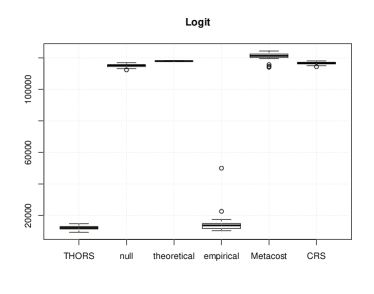
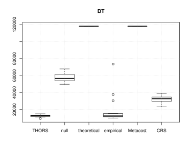
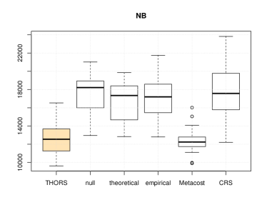
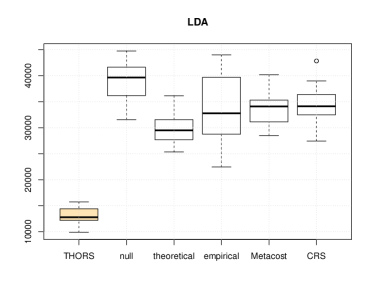
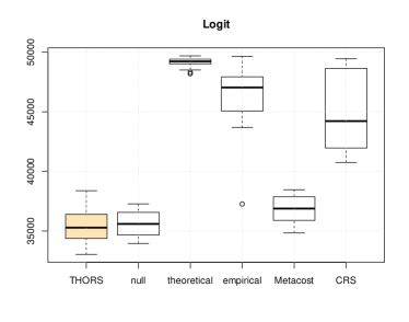
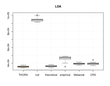
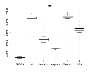
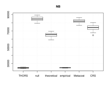
Figure 1: Box-plots of Costs on Test Data by Different Methods for Trucks Data
Table 3: Summary of the Experimental Results for Trucks Data

(An entry w/l𝑤𝑙w/l means THORS wins w𝑤w times and lose l𝑙l times) Base Classifier Algorithm Theoretical Null Empirical Metacost CRS Logit 20/0 20/0 15/5 20/0 20/0 DT 20/0 20/0 10/10 20/0 20/0 NB 20/0 20/0 20/0 8/12 20/0 LDA 20/0 20/0 20/0 20/0 20/0

We list average costs and their deviance for each algorithm on each classifier in Table 2, from which we can see that for Logit, DT, and LDA classifier, THORS reaches the least average cost with small deviance in various methods. Figure 1 exhibited average costs and their deviance for each algorithm on each classifier, from which we can see that for Logit, DT, and LDA classifier, THORS reaches the least average cost with small deviance in various methods. Figure 2 presents the box-plots of cost for each approach on different classifiers. It’s obvious to see that the box-plot of THORS is always at the bottom, which means that THORS is always among the best algorithms for various classifiers. And Table 3 reports the detailed comparison results. THORS wins at least half of 20 rounds in almost all cases (except for Metacost method on NB classifier), beating other strategies in these cases.

Table 4: Average Running Time of Some Methods for Trucks Data (unit: s)
Base Algorithm Thresholding THORS Empirical Metacost CRS
Logit 1.60 17.61 6.92 0.27
DT 2.93 45.60 33.06 0.94
NB 1.33 11.77 0.71 0.07
LDA 1.60 13.25 1.98 0.10
Refer to caption
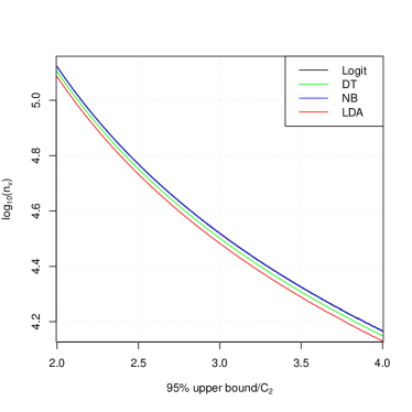
Figure 2: Size of Validation Set and Upper Bound of Cost for Trucks Data

Average running time for one round of each algorithm is listed in Table 4. And relationship between estimated minimal size of validation set (after logarithmic transform), nvsubscript𝑛𝑣n_{v}, and 95% upper bound are exhibited in Figure 2. From Table 4, it is noticed that THORS is always more time-economic in the comparison with Metacost and empirical method. Although CRS always takes the least time due to its simple re-sampling procedure, the performance of it is always much worse than that of THORS. Finally from Figure 2, it’s available to control 95% upper bound under 3.5C23.5subscript𝐶23.5C_{2} for four classifiers using present 24,000 instances in validation set by THORS. We can see that four curves are approximately straight lines, showing an exponential relation between the upper bound and validation set size. And it’s a tradeoff for the increasing sample size and a tighter upper bound. There is no obvious difference for the requirements of validation set size under the same ratio between the upper bound and C2subscript𝐶2C_{2} between four classifiers for THORS algorithm.

4.2 Income Data

The second dataset we choose is an adult dataset containing 32,561 income observations from UCI Machine Learning Repository. Samples belong to two classes: 24,720 people whose income is below 50,000 (class 0, negative) and 7,841 ones whose income is over 50,000 (class 1, positive). The imbalance rate here is 3.15:1, much smaller than the first dataset. We also choose 10 predictors as predictors from 14 other characteristics of each person applying ANOVA F-value, for training base classifiers. To create a cost-sensitive problem we let cost for FN and FP be 100 and 10, respectively. Among these 32,561 observations, 13,025 instances are used to train base models, 13,024 are utilized for thresholding, and remained 6,512 samples are for evaluating the performance of these approaches. Base classifiers we choose are logistic regression with cost weighting (Logit), Naïve Bayes (NB), linear discriminant analysis (LDA), and random forest (RF). We also make a comparison of the performance of THORS with other thresholding schemes such as empirical thresholding method, theoretical thresholding, and other meta-learning strategies, including Metacost and CRS. And each algorithm is also run for 20 times.

Table 5: Average Costs and Standard Deviations for Each Algorithm on Each Classifier for Income Data
THORS Null Theoretical Empirical Metacost CRS
Logit 35469±1371plus-or-minus35469137135469\pm 1371 35584±1066plus-or-minus35584106635584\pm 1066 49144±400plus-or-minus4914440049144\pm 400 46176±2593plus-or-minus46176259346176\pm 2593 36817±1117plus-or-minus36817111736817\pm 1117 44717±3190plus-or-minus44717319044717\pm 3190
LDA 35689±934plus-or-minus3568993435689\pm 934 95099±2497plus-or-minus95099249795099\pm 2497 36252±967plus-or-minus3625296736252\pm 967 45749±3417plus-or-minus45749341745749\pm 3417 39382±1009plus-or-minus39382100939382\pm 1009 39492±1603plus-or-minus39492160339492\pm 1603
NB 32901±934plus-or-minus3290193432901\pm 934 108761±2883plus-or-minus1087612883108761\pm 2883 67100±3360plus-or-minus67100336067100\pm 3360 49455±303plus-or-minus4945530349455\pm 303 110869±2667plus-or-minus1108692667110869\pm 2667 88787±5488plus-or-minus88787548888787\pm 5488
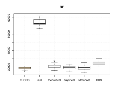
RF 29419±779plus-or-minus2941977929419\pm 779 57135±2131plus-or-minus57135213157135\pm 2131 30415±1338plus-or-minus30415133830415\pm 1338 29507±1172plus-or-minus29507117229507\pm 1172 29769±1497plus-or-minus29769149729769\pm 1497 32378±1185plus-or-minus32378118532378\pm 1185
Refer to caption Refer to caption
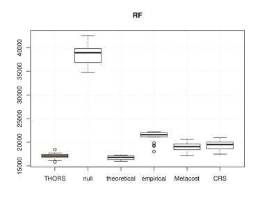
Figure 3: Box-plots of Costs by Different Thresholding Methods
Table 6: Summary of the Experimental Results for Income Data

(An entry w/l means our approach win w times and lose l times) Base Algorithm Thresholding Theoretical Null Empirical Metacost CRS Logit 20/0 12/8 20/0 18/2 20/0 LDA 18/2 20/0 20/0 20/0 20/0 NB 20/0 20/0 20/0 20/0 20/0 RF 17/3 20/0 13/7 11/9 20/0

Table 5 shows the average costs and corresponding deviance on the test set of various thresholding and meta-learning approaches. And win/loss comparison results are summarized in Table 6, from which we can notice that THORS can always beat other methods in more than half of 20 rounds. In addition, THORS even wins all the 20 rounds for NB base classifier in the comparison with all other algorithms. We can see that for all the four classifiers, THORS always gets the minimal average cost with small deviance, showing the power of THORS. Box-plots for different approaches are shown in Figure 3, from which it can be observed that box-plot of THORS always stays near the bottom, representing a low cost on test set.

Table 7: Average Running Time of Some Methods (unit: s)
Base Algorithm Thresholding THORS Empirical Metacost CRS
Logit 1.01 15.88 41.51 0.66
LDA 0.98 13.11 27.88 0.46
NB 0.83 10.94 0.43 0.05
RF 1.32 54.39 13.84 0.53
Refer to caption
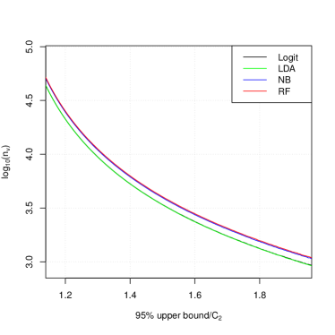
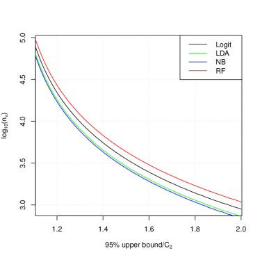
Figure 4: Minimal size of validation Set under 95% specific upper bound

Table 7 exhibits the average running time for a single round for various cost-sensitive algorithms, showing us that THORS is very efficient. And Figure 4 presents the relation between 95% upper bound and the conservative estimation of minimal size of validation set. We can see the similar approximately linear relation between the logarithmic size and the upper bound as in the previous case. It’s easy to control the expected costs under 1.3C2subscript𝐶2C_{2} in the probability of 95% for the present validation set size. And the size will also boom when the upper bound decreases. This result also indicates the trade-off we mentioned in the case of the trucks data set.

4.3 Telescope Data

In this case, we investigate the MAGIC gamma telescope data, which is from UCI Machine Learning Repository. All the 19,020 instances are divided into two classes, including 12,332 class 0 samples and 6,688 class 1 ones. The imbalance rate is 1.84:1. Except for classes, there are 10 other attributes, which will be set as predictors in the models. To formulate this problem into a cost-sensitive one, we set the costs as 100 and 20 for False Negative case and False Positive case. Among 19,020 instances, 7,608 observations are used for training base classifier, denoted as training set, 7,608 ones are applied to choose the optimal threshold, denoted as validation set, and remained 3,804 observations are set as the test set. And the base classifiers we choose include logistic regression with cost weighting (Logit), linear discriminant analysis (LDA), Naïve Bayes (NB), and random forest (RF). The same as previous two datasets, we will compare results of THORS with other thresholding methods, including the null model, theoretical method and empirical method, and other meta-learning approaches, including Metacost and CRS. Each algorithm is also run for 20 rounds.

Table 8: Average Costs and Standard Deviations for Each Algorithm on Each Classifier for Telescope Data
THORS Null Theoretical Empirical Metacost CRS
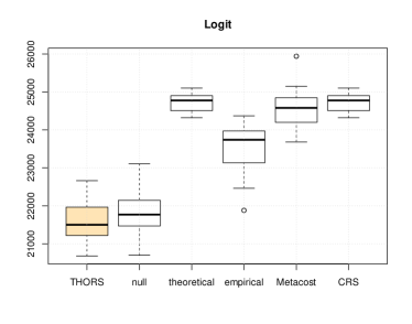
Logit 21773±544plus-or-minus2177354421773\pm 544 24713±241plus-or-minus2471324124713\pm 241 23534±592plus-or-minus2353459223534\pm 592 21606±586plus-or-minus2160658621606\pm 586 24565±514plus-or-minus2456551424565\pm 514 24713±241plus-or-minus2471324124713\pm 241
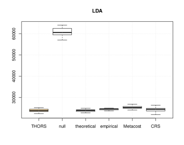
LDA 23924±713plus-or-minus2392471323924\pm 713 60858±2028plus-or-minus60858202860858\pm 2028 23833±600plus-or-minus2383360023833\pm 600 24500±351plus-or-minus2450035124500\pm 351 25301±595plus-or-minus2530159525301\pm 595 24334±910plus-or-minus2433491024334\pm 910
NB 24613±532plus-or-minus2461353224613\pm 532 84904±2550plus-or-minus84904255084904\pm 2550 65014±2675plus-or-minus65014267565014\pm 2675 24713±241plus-or-minus2471324124713\pm 241 82121±2291plus-or-minus82121229182121\pm 2291 73854±3756plus-or-minus73854375673854\pm 3756
RF 16948±596plus-or-minus1694859616948\pm 596 32836±2131plus-or-minus32836213132836\pm 2131 16633±394plus-or-minus1663339416633\pm 394 20142±1080plus-or-minus20142108020142\pm 1080 17735±802plus-or-minus1773580217735\pm 802 18313±982plus-or-minus1831398218313\pm 982
Refer to caption Refer to caption
Figure 5: Box-plots of Costs by Different Thresholding Methods for Telescope Data
Table 9: Summary of the Experimental Results for Telescope Data

(An entry w/l𝑤𝑙w/l means our approach win w𝑤w times and lose l𝑙l times) Base Algorithm Thresholding Theoretical Null Empirical Metacost CRS Logit 20/0 13/7 20/0 20/0 20/0 LDA 9/11 20/0 16/4 19/1 16/4 NB 20/0 20/0 13/7 20/0 20/0 RF 7/13 20/0 20/0 20/0 19/1

It can be noticed from Table 9 that for almost all the cases, THORS defeats other methods over half of 20 rounds (except for theoretical method for LDA and RF classifier). And from Table 8, we can observe that the difference between average costs of THORS and theoretical method for LDA and RF classifier is very small. We can also see from Figure 5 that box-plot of THORS always stay at the bottom of the figure.

Table 10: Average Running Time of Some Methods (unit: s)
Base Algorithm Thresholding THORS Empirical Metacost CRS
Logit 0.55 11.45 14.74 0.56
LDA 0.50 9.51 9.93 0.39
NB 0.48 9.10 7.52 0.30
RF 0.77 37.98 24.85 0.34
Refer to caption
Figure 6: Minimal size of validation Set under 95% specific upper bound

Table 10 lists all the average running times for each algorithm, and from this we can observe that THORS is very efficient. And Figure 6 shows us that it is possible to control the expected cost under about 1.3C21.3subscript𝐶21.3C_{2} in 95% probability for the present validation set size. Under the same ratio between upper bound and C2subscript𝐶2C_{2}, RF classifier seems to need a little more samples in the validation set than other three base classifiers.

5 Discussion

We propose an effective and efficient thresholding algorithm THORS to make an arbitrary scoring-type classifier whose cumulative distribution function of scores is continuous into a cost-sensitive one. Its idea of using order statistic to classify is intuitive and simple. THORS usually results in an excellent performance in terms of cost and time complexity. It can always induce the lowest cost in a short time among various algorithms. Besides, different from other popular cost-sensitive methods, we prove that THORS has several theoretical properties including the bound of the expected cost and an asymptotic boundary, which can also be used to estimate the size of validation to find optimal threshold controlling the expected cost with a specific probability. Finally, THORS often achieves drastic savings in computational resources for its low time complexity, which is desirable for applications that involve a massive amount of data.

One direction for the future work is the application of THORS to multiclass cost-sensitive problems. Here we introduce a simple idea for extending THORS to multiclass cases. Supposed that we have m𝑚m classes noted as class 1,2,,m12𝑚1,2,...,m. And the costs of misclassifying them are decreasing correspondingly. Then we will find an optimal threshold vector with length m1𝑚1m-1. Here the full data is also divided into the training set and validation set to train base models and find optimal thresholds, respectively. Firstly we can sort the misclassification cost of different classes by decreasing order s1,,smsubscript𝑠1subscript𝑠𝑚s_{1},...,s_{m}. Next, we apply THORS on the validation set in terms of class s1subscript𝑠1s_{1} to get a threshold, c1subscript𝑐1c_{1}. Estimated expected cost on validation set can be similarly defined as (2). Then optimal order statistic of one score corresponding to minimal empirical expected cost will be picked up as the first threshold. Next, we can apply THORS again on remained unlabeled observations in validation set and get the second threshold c2subscript𝑐2c_{2}. Similarly, all m1𝑚1m-1 thresholds c1,c2,,cm1subscript𝑐1subscript𝑐2subscript𝑐𝑚1c_{1},c_{2},...,c_{m-1} will be determined. With the threshold vector c=(c1,c2,,cm1)𝑐subscript𝑐1subscript𝑐2subscript𝑐𝑚1c=(c_{1},c_{2},...,c_{m-1}), we can construct the following cost-sensitive classifier: Given a new data point, we firstly decide whether it should be classified into class s1subscript𝑠1s_{1} or not on the basis of c1subscript𝑐1c_{1}. If it does not fall into class s1subscript𝑠1s_{1}, then we calculate the score estimating its possibility belonging to class s2subscript𝑠2s_{2} and assign it to class s2subscript𝑠2s_{2} if the score is lower than c2subscript𝑐2c_{2}. The process holds on until the instance is labeled. Another interesting problem is the case that the cumulative distribution function of the score is not continuous. There may be other ways to yield comparable conclusions in discontinuity case. Besides, THORS can be combined with other approaches like resampling, which may lead to a better performance for imbalanced problem.

Acknowledgments

This work is supported by the National Key Research and Development Plan (No. 2016YFC0800100) and the NSF of China (No. 11671374, 71771203).

References

  • Balakrishnama and Ganapathiraju, (1998) Balakrishnama, S. and Ganapathiraju, A. (1998). Linear discriminant analysis-a brief tutorial. Institute for Signal and information Processing, 18:1–8.
  • Bennett, (1962) Bennett, G. (1962). Probability inequalities for the sum of independent random variables. Journal of the American Statistical Association, 57(297):33–45.
  • Chai et al., (2004) Chai, X., Deng, L., Yang, Q., and Ling, C. X. (2004). Test-cost sensitive naive bayes classification. In null, pages 51–58. IEEE.
  • Domingos, (1999) Domingos, P. (1999). Metacost: A general method for making classifiers cost-sensitive. In Proceedings of the fifth ACM SIGKDD international conference on Knowledge discovery and data mining, pages 155–164. ACM.
  • Drummond and Holte, (2000) Drummond, C. and Holte, R. C. (2000). Exploiting the cost (in) sensitivity of decision tree splitting criteria. In ICML, volume 1.
  • Elkan, (2001) Elkan, C. (2001). The foundations of cost-sensitive learning. In International joint conference on artificial intelligence, volume 17, pages 973–978. Lawrence Erlbaum Associates Ltd.
  • Fan et al., (1999) Fan, W., Stolfo, S. J., Zhang, J., and Chan, P. K. (1999). Adacost: misclassification cost-sensitive boosting. In Icml, pages 97–105.
  • Hoeffding, (1963) Hoeffding, W. (1963). Probability inequalities for sums of bounded random variables. Journal of the American statistical association, 58(301):13–30.
  • Krizhevsky et al., (2012) Krizhevsky, A., Sutskever, I., and Hinton, G. E. (2012). Imagenet classification with deep convolutional neural networks. In Advances in neural information processing systems, pages 1097–1105.
  • McCallum et al., (1998) McCallum, A., Nigam, K., et al. (1998). A comparison of event models for naive bayes text classification. In AAAI-98 workshop on learning for text categorization, volume 752, pages 41–48. Citeseer.
  • Safavian and Landgrebe, (1991) Safavian, S. R. and Landgrebe, D. (1991). A survey of decision tree classifier methodology. IEEE transactions on systems, man, and cybernetics, 21(3):660–674.
  • Sheng and Ling, (2006) Sheng, V. S. and Ling, C. X. (2006). Thresholding for making classifiers cost-sensitive. In AAAI, pages 476–481.
  • Sheng and Ling, (2009) Sheng, V. S. and Ling, C. X. (2009). Cost-sensitive learning. In Encyclopedia of Data Warehousing and Mining, Second Edition, pages 339–345. IGI Global.
  • Sun et al., (2007) Sun, Y., Kamel, M. S., Wong, A. K., and Wang, Y. (2007). Cost-sensitive boosting for classification of imbalanced data. Pattern Recognition, 40(12):3358–3378.
  • Ting, (1998) Ting, K. M. (1998). Inducing cost-sensitive trees via instance weighting. In European Symposium on Principles of Data Mining and Knowledge Discovery, pages 139–147. Springer.
  • Tong et al., (2018) Tong, X., Feng, Y., and Li, J. J. (2018). Neyman-pearson classification algorithms and np receiver operating characteristics. Science advances, 4(2):eaao1659.
  • Turney, (1994) Turney, P. D. (1994). Cost-sensitive classification: Empirical evaluation of a hybrid genetic decision tree induction algorithm. Journal of artificial intelligence research, 2:369–409.
  • Viaene and Dedene, (2005) Viaene, S. and Dedene, G. (2005). Cost-sensitive learning and decision making revisited. European journal of operational research, 166(1):212–220.
  • Witten et al., (2016) Witten, I. H., Frank, E., Hall, M. A., and Pal, C. J. (2016). Data Mining: Practical machine learning tools and techniques. Morgan Kaufmann.
  • Wu, (2005) Wu, S. (2005). Some results on extending and sharpening the weierstrass product inequalities. Journal of mathematical analysis and applications, 308(2):689–702.
  • Zadrozny and Elkan, (2001) Zadrozny, B. and Elkan, C. (2001). Learning and making decisions when costs and probabilities are both unknown. In Proceedings of the seventh ACM SIGKDD international conference on Knowledge discovery and data mining, pages 204–213. ACM.
  • Zadrozny et al., (2003) Zadrozny, B., Langford, J., and Abe, N. (2003). Cost-sensitive learning by cost-proportionate example weighting. In Data Mining, 2003. ICDM 2003. Third IEEE International Conference on, pages 435–442. IEEE.
  • Zhao, (2008) Zhao, H. (2008). Instance weighting versus threshold adjusting for cost-sensitive classification. Knowledge and Information Systems, 15(3):321–334.
  • Zonneveldt et al., (2010) Zonneveldt, S., Korb, K., and Nicholson, A. (2010). Bayesian network classifiers for the german credit data. Technical report, Technical report, Technical report, 2010/1, Bayesian Intelligence. http://www. Bayesian-intelligence. com/publications. php.

Appendix: Proofs

Proof of Theorem 1

Proof.

For (3) and the relation between k0,k1subscript𝑘0subscript𝑘1k_{0},k_{1} and k𝑘k illustrated in Theorem 2.1, class 0 observations scored as T(k0+1)0,T(k0+2)0,,T(n0)0subscriptsuperscript𝑇0subscript𝑘01subscriptsuperscript𝑇0subscript𝑘02subscriptsuperscript𝑇0subscript𝑛0T^{0}_{(k_{0}+1)},T^{0}_{(k_{0}+2)},...,T^{0}_{(n_{0})} will be classified into class 1 and class 1 observations scored as T(1)1,T(2)1,,T(k1)1subscriptsuperscript𝑇11subscriptsuperscript𝑇12subscriptsuperscript𝑇1subscript𝑘1T^{1}_{(1)},T^{1}_{(2)},...,T^{1}_{(k_{1})} will be classified into class 0 if we choose T(k)subscript𝑇𝑘T_{(k)} as the threshold. Then empirical False Negative Rate (FNR) denoted as α^1subscript^𝛼1\widehat{\alpha}_{1} and empirical False Positive Rate (FPR) denoted as α^0subscript^𝛼0\widehat{\alpha}_{0} on validation set satisfy

α^i0=n0k0n0,subscript^𝛼𝑖0subscript𝑛0subscript𝑘0subscript𝑛0\widehat{\alpha}_{i0}=\frac{n_{0}-k_{0}}{n_{0}}, (A.1)
α^i1=k1n1.subscript^𝛼𝑖1subscript𝑘1subscript𝑛1\widehat{\alpha}_{i1}=\frac{k_{1}}{n_{1}}. (A.2)

And for each instance, the cost can be expressed as

C(j,k)={βA,j=0andk=1A,j=1andk=00,otherwise.𝐶𝑗𝑘cases𝛽𝐴absent𝑗0𝑎𝑛𝑑𝑘1𝐴absent𝑗1𝑎𝑛𝑑𝑘00absent𝑜𝑡𝑒𝑟𝑤𝑖𝑠𝑒C(j,k)=\left\{\begin{array}[]{rcl}\beta A&,&j=0\,\,and\,\,k=1\\ A&,&j=1\,\,and\,\,k=0\\ 0&,&otherwise.\\ \end{array}\right. (A.3)

And the marginal probabilities of class 0 and 1, are estimated as π^0=n0nvsubscript^𝜋0subscript𝑛0subscript𝑛𝑣\widehat{\pi}_{0}=\frac{n_{0}}{n_{v}} and π^1=n1nvsubscript^𝜋1subscript𝑛1subscript𝑛𝑣\widehat{\pi}_{1}=\frac{n_{1}}{n_{v}}. Thus, by (2), the expected cost on validation set satisfies

C^^𝐶\displaystyle\widehat{C} =i=1nv[C(0,1)α^i0π^0+C(1,0)α^i1π^1]=i=1nv(βAπ^0α^i0+Aπ^1α^i1)absentsuperscriptsubscript𝑖1subscript𝑛𝑣delimited-[]𝐶01subscript^𝛼𝑖0subscript^𝜋0𝐶10subscript^𝛼𝑖1subscript^𝜋1superscriptsubscript𝑖1subscript𝑛𝑣𝛽𝐴subscript^𝜋0subscript^𝛼𝑖0𝐴subscript^𝜋1subscript^𝛼𝑖1\displaystyle=\sum_{i=1}^{n_{v}}[C(0,1)\widehat{\alpha}_{i0}\widehat{\pi}_{0}+C(1,0)\widehat{\alpha}_{i1}\widehat{\pi}_{1}]=\sum_{i=1}^{n_{v}}(\beta A\widehat{\pi}_{0}\widehat{\alpha}_{i0}+A\widehat{\pi}_{1}\widehat{\alpha}_{i1}) (A.4)
=nvA(βπ^0+π^1k1n1βπ^0k0n0)absentsubscript𝑛𝑣𝐴𝛽subscript^𝜋0subscript^𝜋1subscript𝑘1subscript𝑛1𝛽subscript^𝜋0subscript𝑘0subscript𝑛0\displaystyle=n_{v}A\Big{(}\beta\widehat{\pi}_{0}+\frac{\widehat{\pi}_{1}k_{1}}{n_{1}}-\frac{\beta\widehat{\pi}_{0}k_{0}}{n_{0}}\Big{)}

which means that we only need to minimize π^1k1n1βπ^0k0n0subscript^𝜋1subscript𝑘1subscript𝑛1𝛽subscript^𝜋0subscript𝑘0subscript𝑛0\frac{\widehat{\pi}_{1}k_{1}}{n_{1}}-\frac{\beta\widehat{\pi}_{0}k_{0}}{n_{0}} to minimize C^^𝐶\widehat{C}. This completes the proof. ∎

Proof of Theorem 2

Proof.

In the following notation “\cong” represents “defined as”. By definitions of k0subscript𝑘0k_{0} and k1subscript𝑘1k_{1} in Theorem 2.1, we know that threshold c=T(k)𝑐subscript𝑇𝑘c=T_{(k)} satisfies

max{T(k0)0,T(k1)1}T(k)min{T(k0+1)0,T(k1+1)1},𝑚𝑎𝑥subscriptsuperscript𝑇0subscript𝑘0subscriptsuperscript𝑇1subscript𝑘1subscript𝑇𝑘𝑚𝑖𝑛subscriptsuperscript𝑇0subscript𝑘01subscriptsuperscript𝑇1subscript𝑘11max\{T^{0}_{(k_{0})},T^{1}_{(k_{1})}\}\leq T_{(k)}\leq min\{T^{0}_{(k_{0}+1)},T^{1}_{(k_{1}+1)}\}, (A.5)

indicating that FPR of instance i𝑖i

αi0subscript𝛼𝑖0\displaystyle\alpha_{i0} =P(Ti>T(k)|class(i)=0)P(Ti>T(k0)0|class(i)=0)absent𝑃subscript𝑇𝑖conditionalsubscript𝑇𝑘𝑐𝑙𝑎𝑠𝑠𝑖0𝑃subscript𝑇𝑖conditionalsubscriptsuperscript𝑇0subscript𝑘0𝑐𝑙𝑎𝑠𝑠𝑖0\displaystyle=P(T_{i}>T_{(k)}|class(i)=0)\leq P(T_{i}>T^{0}_{(k_{0})}|class(i)=0) (A.6)
P(Ti0>T(k0)0)=yi0,absent𝑃subscriptsuperscript𝑇0𝑖subscriptsuperscript𝑇0subscript𝑘0subscript𝑦𝑖0\displaystyle\cong P(T^{0}_{i}>T^{0}_{(k_{0})})=y_{i0},

and also

αi0subscript𝛼𝑖0\displaystyle\alpha_{i0} =P(Ti>T(k)|class(i)=0)P(Ti>T(k0+1)0|class(i)=0)absent𝑃subscript𝑇𝑖conditionalsubscript𝑇𝑘𝑐𝑙𝑎𝑠𝑠𝑖0𝑃subscript𝑇𝑖conditionalsubscriptsuperscript𝑇0subscript𝑘01𝑐𝑙𝑎𝑠𝑠𝑖0\displaystyle=P(T_{i}>T_{(k)}|class(i)=0)\geq P(T_{i}>T^{0}_{(k_{0}+1)}|class(i)=0) (A.7)
P(Ti0>T(k0+1)0)=zi0.absent𝑃subscriptsuperscript𝑇0𝑖subscriptsuperscript𝑇0subscript𝑘01subscript𝑧𝑖0\displaystyle\cong P(T^{0}_{i}>T^{0}_{(k_{0}+1)})=z_{i0}.

Similarly, for FNR denoted as αi1subscript𝛼𝑖1\alpha_{i1}, we have

αi1subscript𝛼𝑖1\displaystyle\alpha_{i1} =P(TiT(k)|class(i)=1)P(TiT(k1+1)1|class(i)=1)absent𝑃subscript𝑇𝑖conditionalsubscript𝑇𝑘𝑐𝑙𝑎𝑠𝑠𝑖1𝑃subscript𝑇𝑖conditionalsubscriptsuperscript𝑇1subscript𝑘11𝑐𝑙𝑎𝑠𝑠𝑖1\displaystyle=P(T_{i}\leq T_{(k)}|class(i)=1)\leq P(T_{i}\leq T^{1}_{(k_{1}+1)}|class(i)=1) (A.8)
P(Ti1T(k1+1)1)=yi1,absent𝑃subscriptsuperscript𝑇1𝑖subscriptsuperscript𝑇1subscript𝑘11subscript𝑦𝑖1\displaystyle\cong P(T^{1}_{i}\leq T^{1}_{(k_{1}+1)})=y_{i1},
αi1subscript𝛼𝑖1\displaystyle\alpha_{i1} =P(TiT(k)|class(i)=1)P(TiT(k1)1|class(i)=1)absent𝑃subscript𝑇𝑖conditionalsubscript𝑇𝑘𝑐𝑙𝑎𝑠𝑠𝑖1𝑃subscript𝑇𝑖conditionalsubscriptsuperscript𝑇1subscript𝑘1𝑐𝑙𝑎𝑠𝑠𝑖1\displaystyle=P(T_{i}\leq T_{(k)}|class(i)=1)\geq P(T_{i}\leq T^{1}_{(k_{1})}|class(i)=1) (A.9)
P(Ti1T(k1)1)=zi1.absent𝑃subscriptsuperscript𝑇1𝑖subscriptsuperscript𝑇1subscript𝑘1subscript𝑧𝑖1\displaystyle\cong P(T^{1}_{i}\leq T^{1}_{(k_{1})})=z_{i1}.

Above all, two types of error can be controlled as

zi0P(Ti0>T(k0+1)0)αi0P(Ti0>T(k0)0)yi0,subscript𝑧𝑖0𝑃subscriptsuperscript𝑇0𝑖subscriptsuperscript𝑇0subscript𝑘01subscript𝛼𝑖0𝑃subscriptsuperscript𝑇0𝑖subscriptsuperscript𝑇0subscript𝑘0subscript𝑦𝑖0\displaystyle z_{i0}\cong P(T^{0}_{i}>T^{0}_{(k_{0}+1)})\leq\alpha_{i0}\leq P(T^{0}_{i}>T^{0}_{(k_{0})})\cong y_{i0}, (A.10)
zi1P(Ti1T(k1)1)αi1P(Ti1T(k1+1)1)yi1.subscript𝑧𝑖1𝑃subscriptsuperscript𝑇1𝑖subscriptsuperscript𝑇1subscript𝑘1subscript𝛼𝑖1𝑃subscriptsuperscript𝑇1𝑖subscriptsuperscript𝑇1subscript𝑘11subscript𝑦𝑖1\displaystyle z_{i1}\cong P(T^{1}_{i}\leq T^{1}_{(k_{1})})\leq\alpha_{i1}\leq P(T^{1}_{i}\leq T^{1}_{(k_{1}+1)})\cong y_{i1}. (A.11)

For the randomness of order statistic, here zi0,zi1,yi0,yi1subscript𝑧𝑖0subscript𝑧𝑖1subscript𝑦𝑖0subscript𝑦𝑖1z_{i0},z_{i1},y_{i0},y_{i1} are all random variables instead of constants. Now let’s investigate distributions of yi1,yi0,zi1,zi0subscript𝑦𝑖1subscript𝑦𝑖0subscript𝑧𝑖1subscript𝑧𝑖0y_{i1},y_{i0},z_{i1},z_{i0}. Firstly we denote the conditional cumulative distribution function P(Tix|class(i)=0)=P(Ti0x)𝑃subscript𝑇𝑖conditional𝑥𝑐𝑙𝑎𝑠𝑠𝑖0𝑃subscriptsuperscript𝑇0𝑖𝑥P(T_{i}\leq x|class(i)=0)=P(T^{0}_{i}\leq x) as F0(x)subscript𝐹0𝑥F_{0}(x) and P(Tix|class(i)=1)=P(Ti1x)𝑃subscript𝑇𝑖conditional𝑥𝑐𝑙𝑎𝑠𝑠𝑖1𝑃subscriptsuperscript𝑇1𝑖𝑥P(T_{i}\leq x|class(i)=1)=P(T^{1}_{i}\leq x) as F1(x)subscript𝐹1𝑥F_{1}(x). Hence,

P(yi0x)𝑃subscript𝑦𝑖0𝑥\displaystyle P(y_{i0}\leq x) =P(P(Ti0>T(k0)0)x)=P(1F0(T(k0)0)x)absent𝑃𝑃subscriptsuperscript𝑇0𝑖subscriptsuperscript𝑇0subscript𝑘0𝑥𝑃1subscript𝐹0subscriptsuperscript𝑇0subscript𝑘0𝑥\displaystyle=P(P(T^{0}_{i}>T^{0}_{(k_{0})})\leq x)=P(1-F_{0}(T^{0}_{(k_{0})})\leq x) (A.12)
=P(F0(T(k0)0)1x)=P(T(k0)0F01(1x))absent𝑃subscript𝐹0subscriptsuperscript𝑇0subscript𝑘01𝑥𝑃subscriptsuperscript𝑇0subscript𝑘0superscriptsubscript𝐹011𝑥\displaystyle=P(F_{0}(T^{0}_{(k_{0})})\geq 1-x)=P(T^{0}_{(k_{0})}\geq F_{0}^{-1}(1-x))
=P(atleast(n0k0+1)ofTi0sarenolessthanF01(1x))absent𝑃𝑎𝑡𝑙𝑒𝑎𝑠𝑡subscript𝑛0subscript𝑘01𝑜𝑓subscriptsuperscript𝑇0𝑖superscript𝑠𝑎𝑟𝑒𝑛𝑜𝑙𝑒𝑠𝑠𝑡𝑎𝑛superscriptsubscript𝐹011𝑥\displaystyle=P(at\,least\,(n_{0}-k_{0}+1)\,\,of\,\,T^{0}_{i}\,{}^{\prime}s\,\,are\,\,no\,\,less\,\,than\,\,F_{0}^{-1}(1-x))
=j=n0k0+1n0(n0j)[1F0(F01(1x))]j[F0(F01(1x))]n0jabsentsuperscriptsubscript𝑗subscript𝑛0subscript𝑘01subscript𝑛0binomialsubscript𝑛0𝑗superscriptdelimited-[]1subscript𝐹0superscriptsubscript𝐹011𝑥𝑗superscriptdelimited-[]subscript𝐹0superscriptsubscript𝐹011𝑥subscript𝑛0𝑗\displaystyle=\sum_{j=n_{0}-k_{0}+1}^{n_{0}}\binom{n_{0}}{j}[1-F_{0}(F_{0}^{-1}(1-x))]^{j}[F_{0}(F_{0}^{-1}(1-x))]^{n_{0}-j}
=j=n0k0+1n0(n0j)xj(1x)n0j,absentsuperscriptsubscript𝑗subscript𝑛0subscript𝑘01subscript𝑛0binomialsubscript𝑛0𝑗superscript𝑥𝑗superscript1𝑥subscript𝑛0𝑗\displaystyle=\sum_{j=n_{0}-k_{0}+1}^{n_{0}}\binom{n_{0}}{j}x^{j}(1-x)^{n_{0}-j},
P(yi1x)𝑃subscript𝑦𝑖1𝑥\displaystyle P(y_{i1}\leq x) =P(P(Ti1T(k1+1)1)x)=P(F1(T(k1+1)1)x)absent𝑃𝑃subscriptsuperscript𝑇1𝑖subscriptsuperscript𝑇1subscript𝑘11𝑥𝑃subscript𝐹1subscriptsuperscript𝑇1subscript𝑘11𝑥\displaystyle=P(P(T^{1}_{i}\leq T^{1}_{(k_{1}+1)})\leq x)=P(F_{1}(T^{1}_{(k_{1}+1)})\leq x) (A.13)
=P(T(k1+1)1F11(x))=P(atleast(k1+1)ofTi1sarenomorethanF11(x))absent𝑃subscriptsuperscript𝑇1subscript𝑘11superscriptsubscript𝐹11𝑥𝑃𝑎𝑡𝑙𝑒𝑎𝑠𝑡subscript𝑘11𝑜𝑓subscriptsuperscript𝑇1𝑖superscript𝑠𝑎𝑟𝑒𝑛𝑜𝑚𝑜𝑟𝑒𝑡𝑎𝑛superscriptsubscript𝐹11𝑥\displaystyle=P(T^{1}_{(k_{1}+1)}\leq F_{1}^{-1}(x))=P(at\,\,least\,\,(k_{1}+1)\,\,of\,\,T^{1}_{i}\,{}^{\prime}s\,\,are\,\,no\,\,more\,\,than\,\,F_{1}^{-1}(x))
=j=k1+1n1(n1j)[F1(F11(x))]j[1F1(F11(x))]n1jabsentsuperscriptsubscript𝑗subscript𝑘11subscript𝑛1binomialsubscript𝑛1𝑗superscriptdelimited-[]subscript𝐹1superscriptsubscript𝐹11𝑥𝑗superscriptdelimited-[]1subscript𝐹1superscriptsubscript𝐹11𝑥subscript𝑛1𝑗\displaystyle=\sum_{j=k_{1}+1}^{n_{1}}\binom{n_{1}}{j}[F_{1}(F_{1}^{-1}(x))]^{j}[1-F_{1}(F_{1}^{-1}(x))]^{n_{1}-j}
=j=k1+1n1(n1j)xj(1x)n1j.absentsuperscriptsubscript𝑗subscript𝑘11subscript𝑛1binomialsubscript𝑛1𝑗superscript𝑥𝑗superscript1𝑥subscript𝑛1𝑗\displaystyle=\sum_{j=k_{1}+1}^{n_{1}}\binom{n_{1}}{j}x^{j}(1-x)^{n_{1}-j}.

Similarly there hold

P(zi0x)=j=n0k0n0(n0j)xj(1x)n0j,𝑃subscript𝑧𝑖0𝑥superscriptsubscript𝑗subscript𝑛0subscript𝑘0subscript𝑛0binomialsubscript𝑛0𝑗superscript𝑥𝑗superscript1𝑥subscript𝑛0𝑗P(z_{i0}\leq x)=\sum_{j=n_{0}-k_{0}}^{n_{0}}\binom{n_{0}}{j}x^{j}(1-x)^{n_{0}-j}, (A.14)
P(zi1x)=j=k1n1(n1j)xj(1x)n1j.𝑃subscript𝑧𝑖1𝑥superscriptsubscript𝑗subscript𝑘1subscript𝑛1binomialsubscript𝑛1𝑗superscript𝑥𝑗superscript1𝑥subscript𝑛1𝑗P(z_{i1}\leq x)=\sum_{j=k_{1}}^{n_{1}}\binom{n_{1}}{j}x^{j}(1-x)^{n_{1}-j}. (A.15)

Connecting (A.10) and (A.11) and distributions of yi1,yi0,zi1,zi0subscript𝑦𝑖1subscript𝑦𝑖0subscript𝑧𝑖1subscript𝑧𝑖0y_{i1},y_{i0},z_{i1},z_{i0}, (6) and (7) hold. This completes the proof. ∎

Proof of Theorem 3

Proof.

The expression of expected cost on test set C𝐶C can be derived in the following. Denoting the cost, true class, predicted class of instance i𝑖i and Ci(1,0)subscript𝐶𝑖10C_{i}(1,0) as Costi,Qi,Q^i𝐶𝑜𝑠subscript𝑡𝑖subscript𝑄𝑖subscript^𝑄𝑖Cost_{i},Q_{i},\widehat{Q}_{i} and A𝐴A, then we have

E(Costi)𝐸𝐶𝑜𝑠subscript𝑡𝑖\displaystyle E(Cost_{i}) =E(Costi|Qi=0)π0+E(Costi|Qi=1)π1,absent𝐸conditional𝐶𝑜𝑠subscript𝑡𝑖subscript𝑄𝑖0subscript𝜋0𝐸conditional𝐶𝑜𝑠subscript𝑡𝑖subscript𝑄𝑖1subscript𝜋1\displaystyle=E(Cost_{i}|Q_{i}=0)\pi_{0}+E(Cost_{i}|Q_{i}=1)\pi_{1}, (A.16)
E(Costi|Qi=0)𝐸conditional𝐶𝑜𝑠subscript𝑡𝑖subscript𝑄𝑖0\displaystyle E(Cost_{i}|Q_{i}=0) =E(Costi|Q^i=1,Qi=0)Pi(1|0)=βAαi0,absent𝐸formulae-sequenceconditional𝐶𝑜𝑠subscript𝑡𝑖subscript^𝑄𝑖1subscript𝑄𝑖0subscript𝑃𝑖conditional10𝛽𝐴subscript𝛼𝑖0\displaystyle=E(Cost_{i}|\widehat{Q}_{i}=1,Q_{i}=0)P_{i}(1|0)=\beta A\alpha_{i0}, (A.17)
E(Costi|Qi=1)𝐸conditional𝐶𝑜𝑠subscript𝑡𝑖subscript𝑄𝑖1\displaystyle E(Cost_{i}|Q_{i}=1) =E(Costi|Q^i=0,Qi=1)Pi(0|1)=Aαi1.absent𝐸formulae-sequenceconditional𝐶𝑜𝑠subscript𝑡𝑖subscript^𝑄𝑖0subscript𝑄𝑖1subscript𝑃𝑖conditional01𝐴subscript𝛼𝑖1\displaystyle=E(Cost_{i}|\widehat{Q}_{i}=0,Q_{i}=1)P_{i}(0|1)=A\alpha_{i1}. (A.18)

Therefore

C=i=1nteE(Costi)=i=1nte(βAαi0π0+Aαi1π1)Ai=1nte(βyi0π0+yi1π1).𝐶superscriptsubscript𝑖1subscript𝑛𝑡𝑒𝐸𝐶𝑜𝑠subscript𝑡𝑖superscriptsubscript𝑖1subscript𝑛𝑡𝑒𝛽𝐴subscript𝛼𝑖0subscript𝜋0𝐴subscript𝛼𝑖1subscript𝜋1𝐴superscriptsubscript𝑖1subscript𝑛𝑡𝑒𝛽subscript𝑦𝑖0subscript𝜋0subscript𝑦𝑖1subscript𝜋1C=\sum_{i=1}^{n_{te}}E(Cost_{i})=\sum_{i=1}^{n_{te}}(\beta A\alpha_{i0}\pi_{0}+A\alpha_{i1}\pi_{1})\leq A\sum_{i=1}^{n_{te}}(\beta y_{i0}\pi_{0}+y_{i1}\pi_{1}). (A.19)

Then we denote βAyi0π0𝛽𝐴subscript𝑦𝑖0subscript𝜋0\beta Ay_{i0}\pi_{0} by Yi0subscript𝑌𝑖0Y_{i0}, Ayi1π1𝐴subscript𝑦𝑖1subscript𝜋1Ay_{i1}\pi_{1} by Yi1subscript𝑌𝑖1Y_{i1} and cumulative distribution function of yi1,yi0subscript𝑦𝑖1subscript𝑦𝑖0y_{i1},y_{i0} by G1,G0subscript𝐺1subscript𝐺0G_{1},G_{0}, respectively. The expectation of yi1subscript𝑦𝑖1y_{i1} and yi0subscript𝑦𝑖0y_{i0} can be derived as

E(yi1)𝐸subscript𝑦𝑖1\displaystyle E(y_{i1}) =01P(yi1>x)𝑑x=01(1G1(x))𝑑x=01j=0k1(n1j)xj(1x)n1jdxabsentsuperscriptsubscript01𝑃subscript𝑦𝑖1𝑥differential-d𝑥superscriptsubscript011subscript𝐺1𝑥differential-d𝑥superscriptsubscript01superscriptsubscript𝑗0subscript𝑘1binomialsubscript𝑛1𝑗superscript𝑥𝑗superscript1𝑥subscript𝑛1𝑗𝑑𝑥\displaystyle=\int_{0}^{1}P(y_{i1}>x)dx=\int_{0}^{1}(1-G_{1}(x))dx=\int_{0}^{1}\sum_{j=0}^{k_{1}}\binom{n_{1}}{j}x^{j}(1-x)^{n_{1}-j}dx (A.20)
=j=0k1(n1j)01xj(1x)n1j𝑑x=j=0k1(n1j)Be(j+1,n1j+1)absentsuperscriptsubscript𝑗0subscript𝑘1binomialsubscript𝑛1𝑗superscriptsubscript01superscript𝑥𝑗superscript1𝑥subscript𝑛1𝑗differential-d𝑥superscriptsubscript𝑗0subscript𝑘1binomialsubscript𝑛1𝑗𝐵𝑒𝑗1subscript𝑛1𝑗1\displaystyle=\sum_{j=0}^{k_{1}}\binom{n_{1}}{j}\int_{0}^{1}x^{j}(1-x)^{n_{1}-j}dx=\sum_{j=0}^{k_{1}}\binom{n_{1}}{j}Be(j+1,n_{1}-j+1)
=j=0k1n1!(n1j)!j!Γ(j+1)Γ(n1j+1)Γ(n1+2)=k1+1n1+1,absentsuperscriptsubscript𝑗0subscript𝑘1subscript𝑛1subscript𝑛1𝑗𝑗Γ𝑗1Γsubscript𝑛1𝑗1Γsubscript𝑛12subscript𝑘11subscript𝑛11\displaystyle=\sum_{j=0}^{k_{1}}\frac{n_{1}!}{(n_{1}-j)!j!}\cdot\frac{\Gamma(j+1)\Gamma(n_{1}-j+1)}{\Gamma(n_{1}+2)}=\frac{k_{1}+1}{n_{1}+1},
E(yi0)𝐸subscript𝑦𝑖0\displaystyle E(y_{i0}) =01P(yi0>x)𝑑x=01(1G0(x))𝑑x=01j=0n0k0(n0j)xj(1x)n0jdxabsentsuperscriptsubscript01𝑃subscript𝑦𝑖0𝑥differential-d𝑥superscriptsubscript011subscript𝐺0𝑥differential-d𝑥superscriptsubscript01superscriptsubscript𝑗0subscript𝑛0subscript𝑘0binomialsubscript𝑛0𝑗superscript𝑥𝑗superscript1𝑥subscript𝑛0𝑗𝑑𝑥\displaystyle=\int_{0}^{1}P(y_{i0}>x)dx=\int_{0}^{1}(1-G_{0}(x))dx=\int_{0}^{1}\sum_{j=0}^{n_{0}-k_{0}}\binom{n_{0}}{j}x^{j}(1-x)^{n_{0}-j}dx (A.21)
=j=0n0k0(n0j)01xj(1x)n1j𝑑x=j=0n0k0(n0j)Be(j+1,n0j+1)absentsuperscriptsubscript𝑗0subscript𝑛0subscript𝑘0binomialsubscript𝑛0𝑗superscriptsubscript01superscript𝑥𝑗superscript1𝑥subscript𝑛1𝑗differential-d𝑥superscriptsubscript𝑗0subscript𝑛0subscript𝑘0binomialsubscript𝑛0𝑗𝐵𝑒𝑗1subscript𝑛0𝑗1\displaystyle=\sum_{j=0}^{n_{0}-k_{0}}\binom{n_{0}}{j}\int_{0}^{1}x^{j}(1-x)^{n_{1}-j}dx=\sum_{j=0}^{n_{0}-k_{0}}\binom{n_{0}}{j}Be(j+1,n_{0}-j+1)
=j=0n0k0n0!(n0j)!j!Γ(j+1)Γ(n0j+1)Γ(n0+2)=n0k0+1n0+1,absentsuperscriptsubscript𝑗0subscript𝑛0subscript𝑘0subscript𝑛0subscript𝑛0𝑗𝑗Γ𝑗1Γsubscript𝑛0𝑗1Γsubscript𝑛02subscript𝑛0subscript𝑘01subscript𝑛01\displaystyle=\sum_{j=0}^{n_{0}-k_{0}}\frac{n_{0}!}{(n_{0}-j)!j!}\cdot\frac{\Gamma(j+1)\Gamma(n_{0}-j+1)}{\Gamma(n_{0}+2)}=\frac{n_{0}-k_{0}+1}{n_{0}+1},
E(yi02)𝐸superscriptsubscript𝑦𝑖02\displaystyle E(y_{i0}^{2}) =01x2𝑑G0(x)=x2G0(x)|01201xG0(x)𝑑x=1201x[1G0¯(x)]𝑑xabsentsuperscriptsubscript01superscript𝑥2differential-dsubscript𝐺0𝑥evaluated-atsuperscript𝑥2subscript𝐺0𝑥012superscriptsubscript01𝑥subscript𝐺0𝑥differential-d𝑥12superscriptsubscript01𝑥delimited-[]1¯subscript𝐺0𝑥differential-d𝑥\displaystyle=\int_{0}^{1}x^{2}dG_{0}(x)=x^{2}G_{0}(x)\arrowvert_{0}^{1}-2\int_{0}^{1}xG_{0}(x)dx=1-2\int_{0}^{1}x[1-\overline{G_{0}}(x)]dx (A.22)
=201xG0¯(x)𝑑x=2j=0n0k0(n0j)01xj+1(1x)n0j𝑑xabsent2superscriptsubscript01𝑥¯subscript𝐺0𝑥differential-d𝑥2superscriptsubscript𝑗0subscript𝑛0subscript𝑘0binomialsubscript𝑛0𝑗superscriptsubscript01superscript𝑥𝑗1superscript1𝑥subscript𝑛0𝑗differential-d𝑥\displaystyle=2\int_{0}^{1}x\overline{G_{0}}(x)dx=2\sum_{j=0}^{n_{0}-k_{0}}\binom{n_{0}}{j}\int_{0}^{1}x^{j+1}(1-x)^{n_{0}-j}dx
=2j=0n0k0(n0j)Be(j+2,n0j+1)=2j=0n0k0n0!(n0j)!j!Γ(j+2)Γ(n0j+1)Γ(n0+3)absent2superscriptsubscript𝑗0subscript𝑛0subscript𝑘0binomialsubscript𝑛0𝑗𝐵𝑒𝑗2subscript𝑛0𝑗12superscriptsubscript𝑗0subscript𝑛0subscript𝑘0subscript𝑛0subscript𝑛0𝑗𝑗Γ𝑗2Γsubscript𝑛0𝑗1Γsubscript𝑛03\displaystyle=2\sum_{j=0}^{n_{0}-k_{0}}\binom{n_{0}}{j}Be(j+2,n_{0}-j+1)=2\sum_{j=0}^{n_{0}-k_{0}}\frac{n_{0}!}{(n_{0}-j)!j!}\cdot\frac{\Gamma(j+2)\Gamma(n_{0}-j+1)}{\Gamma(n_{0}+3)}
=(n0k0+1)(n0k0+2)(n0+1)(n0+2),absentsubscript𝑛0subscript𝑘01subscript𝑛0subscript𝑘02subscript𝑛01subscript𝑛02\displaystyle=\frac{(n_{0}-k_{0}+1)(n_{0}-k_{0}+2)}{(n_{0}+1)(n_{0}+2)},
E(yi12)𝐸superscriptsubscript𝑦𝑖12\displaystyle E(y_{i1}^{2}) =01x2𝑑G1(x)=x2G1(x)|01201xG1(x)𝑑x=1201x[1G1¯(x)]𝑑xabsentsuperscriptsubscript01superscript𝑥2differential-dsubscript𝐺1𝑥evaluated-atsuperscript𝑥2subscript𝐺1𝑥012superscriptsubscript01𝑥subscript𝐺1𝑥differential-d𝑥12superscriptsubscript01𝑥delimited-[]1¯subscript𝐺1𝑥differential-d𝑥\displaystyle=\int_{0}^{1}x^{2}dG_{1}(x)=x^{2}G_{1}(x)\arrowvert_{0}^{1}-2\int_{0}^{1}xG_{1}(x)dx=1-2\int_{0}^{1}x[1-\overline{G_{1}}(x)]dx (A.23)
=201xG1¯(x)𝑑x=2j=0k1(n1j)01xj+1(1x)n1j𝑑x=2j=0k1(n1j)Be(j+2,n1j+1)absent2superscriptsubscript01𝑥¯subscript𝐺1𝑥differential-d𝑥2superscriptsubscript𝑗0subscript𝑘1binomialsubscript𝑛1𝑗superscriptsubscript01superscript𝑥𝑗1superscript1𝑥subscript𝑛1𝑗differential-d𝑥2superscriptsubscript𝑗0subscript𝑘1binomialsubscript𝑛1𝑗𝐵𝑒𝑗2subscript𝑛1𝑗1\displaystyle=2\int_{0}^{1}x\overline{G_{1}}(x)dx=2\sum_{j=0}^{k_{1}}\binom{n_{1}}{j}\int_{0}^{1}x^{j+1}(1-x)^{n_{1}-j}dx=2\sum_{j=0}^{k_{1}}\binom{n_{1}}{j}Be(j+2,n_{1}-j+1)
=2j=0k1n1!(n1j)!j!Γ(j+2)Γ(n1j+1)Γ(n1+3)=(k1+2)(k1+1)(n1+2)(n1+1).absent2superscriptsubscript𝑗0subscript𝑘1subscript𝑛1subscript𝑛1𝑗𝑗Γ𝑗2Γsubscript𝑛1𝑗1Γsubscript𝑛13subscript𝑘12subscript𝑘11subscript𝑛12subscript𝑛11\displaystyle=2\sum_{j=0}^{k_{1}}\frac{n_{1}!}{(n_{1}-j)!j!}\cdot\frac{\Gamma(j+2)\Gamma(n_{1}-j+1)}{\Gamma(n_{1}+3)}=\frac{(k_{1}+2)(k_{1}+1)}{(n_{1}+2)(n_{1}+1)}.

The variance of yi1,yi0subscript𝑦𝑖1subscript𝑦𝑖0y_{i1},y_{i0} can be expressed as

Var(yi1)𝑉𝑎𝑟subscript𝑦𝑖1\displaystyle Var(y_{i1}) =E(yi12)(Eyi1)2absent𝐸superscriptsubscript𝑦𝑖12superscript𝐸subscript𝑦𝑖12\displaystyle=E(y_{i1}^{2})-(Ey_{i1})^{2} =(k1+1)(n1k1)(n1+1)2(n1+2),absentsubscript𝑘11subscript𝑛1subscript𝑘1superscriptsubscript𝑛112subscript𝑛12\displaystyle=\frac{(k_{1}+1)(n_{1}-k_{1})}{(n_{1}+1)^{2}(n_{1}+2)}, (A.24)
Var(yi0)𝑉𝑎𝑟subscript𝑦𝑖0\displaystyle Var(y_{i0}) =E(yi02)(Eyi0)2absent𝐸superscriptsubscript𝑦𝑖02superscript𝐸subscript𝑦𝑖02\displaystyle=E(y_{i0}^{2})-(Ey_{i0})^{2} =k0(n0k0+1)(n0+1)2(n0+2).absentsubscript𝑘0subscript𝑛0subscript𝑘01superscriptsubscript𝑛012subscript𝑛02\displaystyle=\frac{k_{0}(n_{0}-k_{0}+1)}{(n_{0}+1)^{2}(n_{0}+2)}. (A.25)

By Bernstein’s inequality (Bennett,, 1962) we have

P(i=1nte[(Yi1EYi1)+(Yi0EYi0)]>tσ)𝑃superscriptsubscript𝑖1subscript𝑛𝑡𝑒delimited-[]subscript𝑌𝑖1𝐸subscript𝑌𝑖1subscript𝑌𝑖0𝐸subscript𝑌𝑖0𝑡𝜎\displaystyle P\Big{(}\sum_{i=1}^{n_{te}}[(Y_{i1}-EY_{i1})+(Y_{i0}-EY_{i0})]>t\sigma\Big{)} (A.26)
exp{12(tσ)2i=1nte[E(Yi1EYi1)2+E(Yi0EYi0)2]+M3tσ}absent𝑒𝑥𝑝12superscript𝑡𝜎2superscriptsubscript𝑖1subscript𝑛𝑡𝑒delimited-[]𝐸superscriptsubscript𝑌𝑖1𝐸subscript𝑌𝑖12𝐸superscriptsubscript𝑌𝑖0𝐸subscript𝑌𝑖02superscript𝑀3𝑡𝜎\displaystyle\leq exp\Bigg{\{}-\frac{\frac{1}{2}(t\sigma)^{2}}{\sum\limits_{i=1}^{n_{te}}[E(Y_{i1}-EY_{i1})^{2}+E(Y_{i0}-EY_{i0})^{2}]+\frac{M^{\prime}}{3}t\sigma}\Bigg{\}}
=exp{12(tσ)2i=1nte[Var(Yi1)+Var(Yi0)]+M3tσ}absent𝑒𝑥𝑝12superscript𝑡𝜎2superscriptsubscript𝑖1subscript𝑛𝑡𝑒delimited-[]𝑉𝑎𝑟subscript𝑌𝑖1𝑉𝑎𝑟subscript𝑌𝑖0superscript𝑀3𝑡𝜎\displaystyle=exp\Bigg{\{}-\frac{\frac{1}{2}(t\sigma)^{2}}{\sum\limits_{i=1}^{n_{te}}[Var(Y_{i1})+Var(Y_{i0})]+\frac{M^{\prime}}{3}t\sigma}\Bigg{\}}
=exp{(tσ)22σ2+2M3tσ}exp{t22+2M3σt}p,absent𝑒𝑥𝑝superscript𝑡𝜎22superscript𝜎22superscript𝑀3𝑡𝜎𝑒𝑥𝑝superscript𝑡222𝑀3𝜎𝑡𝑝\displaystyle=exp\Bigg{\{}-\frac{(t\sigma)^{2}}{2\sigma^{2}+\frac{2M^{\prime}}{3}t\sigma}\Bigg{\}}\leq exp\Bigg{\{}-\frac{t^{2}}{2+\frac{2M}{3\sigma}t}\Bigg{\}}\cong p,

where

σ2superscript𝜎2\displaystyle\sigma^{2} =i=1nte[Var(Yi1)+Var(Yi0)]=i=1nte[(π1A)2Var(yi1)+(βπ0A)2Var(yi0)]absentsuperscriptsubscript𝑖1subscript𝑛𝑡𝑒delimited-[]𝑉𝑎𝑟subscript𝑌𝑖1𝑉𝑎𝑟subscript𝑌𝑖0superscriptsubscript𝑖1subscript𝑛𝑡𝑒delimited-[]superscriptsubscript𝜋1𝐴2𝑉𝑎𝑟subscript𝑦𝑖1superscript𝛽subscript𝜋0𝐴2𝑉𝑎𝑟subscript𝑦𝑖0\displaystyle=\sum_{i=1}^{n_{te}}[Var(Y_{i1})+Var(Y_{i0})]=\sum_{i=1}^{n_{te}}[(\pi_{1}A)^{2}Var(y_{i1})+(\beta\pi_{0}A)^{2}Var(y_{i0})] (A.27)
=nteA2[π12Var(yi1)+(βπ0)2Var(yi0)]absentsubscript𝑛𝑡𝑒superscript𝐴2delimited-[]superscriptsubscript𝜋12𝑉𝑎𝑟subscript𝑦𝑖1superscript𝛽subscript𝜋02𝑉𝑎𝑟subscript𝑦𝑖0\displaystyle=n_{te}A^{2}\Big{[}\pi_{1}^{2}Var(y_{i1})+(\beta\pi_{0})^{2}Var(y_{i0})\Big{]}
=nteA2[π12(k1+1)(n1k1)(n1+1)2(n1+2)+(βπ0)2k0(n0k0+1)(n0+1)2(n0+2)],absentsubscript𝑛𝑡𝑒superscript𝐴2delimited-[]superscriptsubscript𝜋12subscript𝑘11subscript𝑛1subscript𝑘1superscriptsubscript𝑛112subscript𝑛12superscript𝛽subscript𝜋02subscript𝑘0subscript𝑛0subscript𝑘01superscriptsubscript𝑛012subscript𝑛02\displaystyle=n_{te}A^{2}\Big{[}\pi_{1}^{2}\frac{(k_{1}+1)(n_{1}-k_{1})}{(n_{1}+1)^{2}(n_{1}+2)}+(\beta\pi_{0})^{2}\frac{k_{0}(n_{0}-k_{0}+1)}{(n_{0}+1)^{2}(n_{0}+2)}\Big{]},
Msuperscript𝑀\displaystyle M^{\prime} =max1inte{|Yi1EYi1|,|Yi0EYi0|}absentsubscript𝑚𝑎𝑥1𝑖subscript𝑛𝑡𝑒subscript𝑌𝑖1𝐸subscript𝑌𝑖1subscript𝑌𝑖0𝐸subscript𝑌𝑖0\displaystyle=\mathop{max}\limits_{1\leq i\leq n_{te}}\{|Y_{i1}-EY_{i1}|,|Y_{i0}-EY_{i0}|\} (A.28)
=Amax1inte{π1|yi1Eyi1|,βπ0|yi0Eyi0|}absent𝐴subscript𝑚𝑎𝑥1𝑖subscript𝑛𝑡𝑒subscript𝜋1subscript𝑦𝑖1𝐸subscript𝑦𝑖1𝛽subscript𝜋0subscript𝑦𝑖0𝐸subscript𝑦𝑖0\displaystyle=A\mathop{max}\limits_{1\leq i\leq n_{te}}\{\pi_{1}|y_{i1}-Ey_{i1}|,\beta\pi_{0}|y_{i0}-Ey_{i0}|\}
Amax1inte{π1|yi1Eyi1|,βπ0|yi0Eyi0|}absent𝐴subscript𝑚𝑎𝑥1𝑖subscript𝑛𝑡𝑒subscript𝜋1subscript𝑦𝑖1𝐸subscript𝑦𝑖1𝛽subscript𝜋0subscript𝑦𝑖0𝐸subscript𝑦𝑖0\displaystyle\leq A\cdot\mathop{max}\limits_{1\leq i\leq n_{te}}\{\pi_{1}|y_{i1}-Ey_{i1}|,\beta\pi_{0}|y_{i0}-Ey_{i0}|\}
Amax{π1(|Eyi1|,|1Eyi1|),βπ0(|Eyi0|,|1Eyi0|)}absent𝐴𝑚𝑎𝑥subscript𝜋1𝐸subscript𝑦𝑖11𝐸subscript𝑦𝑖1𝛽subscript𝜋0𝐸subscript𝑦𝑖01𝐸subscript𝑦𝑖0\displaystyle\leq A\cdot max\{\pi_{1}(|Ey_{i1}|,|1-Ey_{i1}|),\beta\pi_{0}(|Ey_{i0}|,|1-Ey_{i0}|)\}
=Amax{π1max(k1+1n1+1,1k1+1n1+1),\displaystyle=A\cdot max\Big{\{}\pi_{1}max\Big{(}\frac{k_{1}+1}{n_{1}+1},1-\frac{k_{1}+1}{n_{1}+1}\Big{)},
βπ0max(n0k0+1n0+1,1n0k0+1n0+1)}M.\displaystyle\beta\pi_{0}max\Big{(}\frac{n_{0}-k_{0}+1}{n_{0}+1},1-\frac{n_{0}-k_{0}+1}{n_{0}+1}\Big{)}\Big{\}}\cong M.

Then we obtain

P(CC+tσ)𝑃𝐶superscript𝐶𝑡𝜎\displaystyle P(C\leq C^{*}+t\sigma) P(i=1nte(Yi1+Yi0)C+tσ)absent𝑃superscriptsubscript𝑖1subscript𝑛𝑡𝑒subscript𝑌𝑖1subscript𝑌𝑖0superscript𝐶𝑡𝜎\displaystyle\geq P\Big{(}\sum_{i=1}^{n_{te}}(Y_{i1}+Y_{i0})\leq C^{*}+t\sigma\Big{)} (A.29)
=1P(i=1nte(Yi1+Yi0)>C+tσ)absent1𝑃superscriptsubscript𝑖1subscript𝑛𝑡𝑒subscript𝑌𝑖1subscript𝑌𝑖0superscript𝐶𝑡𝜎\displaystyle=1-P\Big{(}\sum_{i=1}^{n_{te}}(Y_{i1}+Y_{i0})>C^{*}+t\sigma\Big{)}
=1P(i=1nte[(Yi1EYi1)+(Yi0EYi0)]>tσ)1p.absent1𝑃superscriptsubscript𝑖1subscript𝑛𝑡𝑒delimited-[]subscript𝑌𝑖1𝐸subscript𝑌𝑖1subscript𝑌𝑖0𝐸subscript𝑌𝑖0𝑡𝜎1𝑝\displaystyle=1-P\Big{(}\sum_{i=1}^{n_{te}}[(Y_{i1}-EY_{i1})+(Y_{i0}-EY_{i0})]>t\sigma\Big{)}\geq 1-p.

This completes the proof. ∎

Proof of Theorem 4

Proof.

We list required time for each step of Algorithm 1.

Table 11: Main Steps of Algorithm 1 and Their Required Time
Step No. Detail Time Scale Coefficient
1 calculate scores O(nv)𝑂subscript𝑛𝑣O(n_{v}) d1subscript𝑑1d_{1}
2 sort O(nvlognv)𝑂subscript𝑛𝑣𝑙𝑜𝑔subscript𝑛𝑣O(n_{v}log\,n_{v}) d20subscript𝑑20d_{2}\approx 0
3 initialize two counters O(1)𝑂1O(1) d3subscript𝑑3d_{3}
4-12 iterate validation set O(nv)𝑂subscript𝑛𝑣O(n_{v}) d4subscript𝑑4d_{4}
13-15 find Lsuperscript𝐿L^{*} and return parameters O(1)𝑂1O(1) d5subscript𝑑5d_{5}

The total running time can be expressed as

Time𝑇𝑖𝑚𝑒\displaystyle Time =d3nvlognv+(d1+d4)nv+d2+d5absentsubscript𝑑3subscript𝑛𝑣𝑙𝑜𝑔subscript𝑛𝑣subscript𝑑1subscript𝑑4subscript𝑛𝑣subscript𝑑2subscript𝑑5\displaystyle=d_{3}n_{v}log\,n_{v}+(d_{1}+d_{4})n_{v}+d_{2}+d_{5} (A.30)
d3nvlognv+(d1+d2+d4+d5)nva1nvlognv+a2nv,absentsubscript𝑑3subscript𝑛𝑣𝑙𝑜𝑔subscript𝑛𝑣subscript𝑑1subscript𝑑2subscript𝑑4subscript𝑑5subscript𝑛𝑣subscript𝑎1subscript𝑛𝑣𝑙𝑜𝑔subscript𝑛𝑣subscript𝑎2subscript𝑛𝑣\displaystyle\leq d_{3}n_{v}log\,n_{v}+(d_{1}+d_{2}+d_{4}+d_{5})n_{v}\cong a_{1}n_{v}log\,n_{v}+a_{2}n_{v},

where a1subscript𝑎1a_{1} is very small. Then we have total time complexity scale as

TimeScale𝑇𝑖𝑚𝑒𝑆𝑐𝑎𝑙𝑒\displaystyle Time\,\,Scale =O(nv)+O(nvlognv)+O(nv)+O(1)=O(nvlognv).absent𝑂subscript𝑛𝑣𝑂subscript𝑛𝑣𝑙𝑜𝑔subscript𝑛𝑣𝑂subscript𝑛𝑣𝑂1𝑂subscript𝑛𝑣𝑙𝑜𝑔subscript𝑛𝑣\displaystyle=O(n_{v})+O(n_{v}log\,n_{v})+O(n_{v})+O(1)=O(n_{v}log\,n_{v}). (A.31)

Proof of Theorem 5

Proof.

Let Hp(n)subscript𝐻𝑝𝑛H_{p}(n) denote the success number of n𝑛n Bernoulli trials with success probability p𝑝p, then there exists

P(yi0>py0+ε)𝑃subscript𝑦𝑖0subscript𝑝𝑦0𝜀\displaystyle P(y_{i0}>p_{y0}+\varepsilon) =j=0n0k0(n0j)(py0+ε)j(1(py0+ε))n0jabsentsuperscriptsubscript𝑗0subscript𝑛0subscript𝑘0binomialsubscript𝑛0𝑗superscriptsubscript𝑝𝑦0𝜀𝑗superscript1subscript𝑝𝑦0𝜀subscript𝑛0𝑗\displaystyle=\sum_{j=0}^{n_{0}-k_{0}}\binom{n_{0}}{j}(p_{y0}+\varepsilon)^{j}(1-(p_{y0}+\varepsilon))^{n_{0}-j} (A.32)
=P(Hpy0+ε(n0)n0k0),absent𝑃subscript𝐻subscript𝑝𝑦0𝜀subscript𝑛0subscript𝑛0subscript𝑘0\displaystyle=P(H_{p_{y0}+\varepsilon}(n_{0})\leq n_{0}-k_{0}),

where py0=Eyi0=n0k0+1n0+1subscript𝑝𝑦0𝐸subscript𝑦𝑖0subscript𝑛0subscript𝑘01subscript𝑛01p_{y0}=Ey_{i0}=\frac{n_{0}-k_{0}+1}{n_{0}+1}. And let py0=py0+εsuperscriptsubscript𝑝𝑦0subscript𝑝𝑦0𝜀p_{y0}^{\prime}=p_{y0}+\varepsilon, n0k0=(py0εy0)n0=(py0+εεy0)n0subscript𝑛0subscript𝑘0superscriptsubscript𝑝𝑦0superscriptsubscript𝜀𝑦0subscript𝑛0subscript𝑝𝑦0𝜀superscriptsubscript𝜀𝑦0subscript𝑛0n_{0}-k_{0}=(p_{y0}^{\prime}-\varepsilon_{y0}^{\prime})n_{0}=(p_{y0}+\varepsilon-\varepsilon_{y0}^{\prime})n_{0}, we will obtain

εy0=k0n0(n0+1)+ε.superscriptsubscript𝜀𝑦0subscript𝑘0subscript𝑛0subscript𝑛01𝜀\varepsilon_{y0}^{\prime}=\frac{k_{0}}{n_{0}(n_{0}+1)}+\varepsilon. (A.33)

Therefore by Hoeffding’s inequality (Hoeffding,, 1963),

P(yi0>py0+ε)𝑃subscript𝑦𝑖0subscript𝑝𝑦0𝜀\displaystyle P(y_{i0}>p_{y0}+\varepsilon) =P(Hpy0(n0)(py0εy0)n0)exp{2(εy0)2n0}absent𝑃subscript𝐻superscriptsubscript𝑝𝑦0subscript𝑛0superscriptsubscript𝑝𝑦0superscriptsubscript𝜀𝑦0subscript𝑛0𝑒𝑥𝑝2superscriptsuperscriptsubscript𝜀𝑦02subscript𝑛0\displaystyle=P(H_{p_{y0}^{\prime}}(n_{0})\leq(p_{y0}^{\prime}-\varepsilon_{y0}^{\prime})n_{0})\leq exp\{-2(\varepsilon_{y0}^{\prime})^{2}n_{0}\} (A.34)
=exp{2[k0n0(n0+1)+ε]2n0},absent𝑒𝑥𝑝2superscriptdelimited-[]subscript𝑘0subscript𝑛0subscript𝑛01𝜀2subscript𝑛0\displaystyle=exp\Big{\{}-2\Big{[}\frac{k_{0}}{n_{0}(n_{0}+1)}+\varepsilon\Big{]}^{2}n_{0}\Big{\}},
P(yi0py0+ε)1exp{2[k0n0(n0+1)+ε]2n0}.𝑃subscript𝑦𝑖0subscript𝑝𝑦0𝜀1𝑒𝑥𝑝2superscriptdelimited-[]subscript𝑘0subscript𝑛0subscript𝑛01𝜀2subscript𝑛0P(y_{i0}\leq p_{y0}+\varepsilon)\geq 1-exp\Big{\{}-2\Big{[}\frac{k_{0}}{n_{0}(n_{0}+1)}+\varepsilon\Big{]}^{2}n_{0}\Big{\}}. (A.35)

For zi0subscript𝑧𝑖0z_{i0} we have

P(zi0<pz0ε)𝑃subscript𝑧𝑖0subscript𝑝𝑧0𝜀\displaystyle P(z_{i0}<p_{z0}-\varepsilon) =j=n0k0n0(n0j)(pz0ε)j(1(pz0ε))n0jabsentsuperscriptsubscript𝑗subscript𝑛0subscript𝑘0subscript𝑛0binomialsubscript𝑛0𝑗superscriptsubscript𝑝𝑧0𝜀𝑗superscript1subscript𝑝𝑧0𝜀subscript𝑛0𝑗\displaystyle=\sum_{j=n_{0}-k_{0}}^{n_{0}}\binom{n_{0}}{j}(p_{z0}-\varepsilon)^{j}(1-(p_{z0}-\varepsilon))^{n_{0}-j} (A.36)
=P(Hpz0ε(n0)n0k0),absent𝑃subscript𝐻subscript𝑝𝑧0𝜀subscript𝑛0subscript𝑛0subscript𝑘0\displaystyle=P(H_{p_{z0}-\varepsilon}(n_{0})\geq n_{0}-k_{0}),

where pz0=Ezi0=n0k0n0+1subscript𝑝𝑧0𝐸subscript𝑧𝑖0subscript𝑛0subscript𝑘0subscript𝑛01p_{z0}=Ez_{i0}=\frac{n_{0}-k_{0}}{n_{0}+1}. Next we let pz0=pz0εsuperscriptsubscript𝑝𝑧0subscript𝑝𝑧0𝜀p_{z0}^{\prime}=p_{z0}-\varepsilon, n0k0=(pz0+εz0)n0=(pz0ε+εz0)n0subscript𝑛0subscript𝑘0superscriptsubscript𝑝𝑧0superscriptsubscript𝜀𝑧0subscript𝑛0subscript𝑝𝑧0𝜀superscriptsubscript𝜀𝑧0subscript𝑛0n_{0}-k_{0}=(p_{z0}^{\prime}+\varepsilon_{z0}^{\prime})n_{0}=(p_{z0}-\varepsilon+\varepsilon_{z0}^{\prime})n_{0}, we will obtain

εz0=n0k0n0(n0+1)+ε.superscriptsubscript𝜀𝑧0subscript𝑛0subscript𝑘0subscript𝑛0subscript𝑛01𝜀\varepsilon_{z0}^{\prime}=\frac{n_{0}-k_{0}}{n_{0}(n_{0}+1)}+\varepsilon. (A.37)

Therefore by Hoeffding’s inequality

P(zi0<pz0ε)𝑃subscript𝑧𝑖0subscript𝑝𝑧0𝜀\displaystyle P(z_{i0}<p_{z0}-\varepsilon) =P(Hpz0(n0)(pz0+εz0)n0)absent𝑃subscript𝐻superscriptsubscript𝑝𝑧0subscript𝑛0superscriptsubscript𝑝𝑧0superscriptsubscript𝜀𝑧0subscript𝑛0\displaystyle=P(H_{p_{z0}^{\prime}}(n_{0})\geq(p_{z0}^{\prime}+\varepsilon_{z0}^{\prime})n_{0}) (A.38)
exp{2(εz0)2n0}=exp{2[n0k0n0(n0+1)+ε]2n0}.absent𝑒𝑥𝑝2superscriptsuperscriptsubscript𝜀𝑧02subscript𝑛0𝑒𝑥𝑝2superscriptdelimited-[]subscript𝑛0subscript𝑘0subscript𝑛0subscript𝑛01𝜀2subscript𝑛0\displaystyle\leq exp\Big{\{}-2(\varepsilon_{z0}^{\prime})^{2}n_{0}\Big{\}}=exp\Big{\{}-2\Big{[}\frac{n_{0}-k_{0}}{n_{0}(n_{0}+1)}+\varepsilon\Big{]}^{2}n_{0}\}.
P(zi0pz0ε)1exp{2[n0k0n0(n0+1)+ε]2n0}.𝑃subscript𝑧𝑖0subscript𝑝𝑧0𝜀1𝑒𝑥𝑝2superscriptdelimited-[]subscript𝑛0subscript𝑘0subscript𝑛0subscript𝑛01𝜀2subscript𝑛0P(z_{i0}\geq p_{z0}-\varepsilon)\geq 1-exp\Big{\{}-2\Big{[}\frac{n_{0}-k_{0}}{n_{0}(n_{0}+1)}+\varepsilon\Big{]}^{2}n_{0}\Big{\}}. (A.39)

Similarly,

P(yi1py1+ε)1exp{2[n1k1n1(n1+1)+ε]2n1},𝑃subscript𝑦𝑖1subscript𝑝𝑦1𝜀1𝑒𝑥𝑝2superscriptdelimited-[]subscript𝑛1subscript𝑘1subscript𝑛1subscript𝑛11𝜀2subscript𝑛1P(y_{i1}\leq p_{y1}+\varepsilon)\geq 1-exp\Big{\{}-2\Big{[}\frac{n_{1}-k_{1}}{n_{1}(n_{1}+1)}+\varepsilon\Big{]}^{2}n_{1}\Big{\}}, (A.40)
P(zi1pz1ε)1exp{2[k1n1(n1+1)+ε]2n1}.𝑃subscript𝑧𝑖1subscript𝑝𝑧1𝜀1𝑒𝑥𝑝2superscriptdelimited-[]subscript𝑘1subscript𝑛1subscript𝑛11𝜀2subscript𝑛1P(z_{i1}\geq p_{z1}-\varepsilon)\geq 1-exp\Big{\{}-2\Big{[}\frac{k_{1}}{n_{1}(n_{1}+1)}+\varepsilon\Big{]}^{2}n_{1}\Big{\}}. (A.41)

where py1=Eyi1=k1+1n1+1subscript𝑝𝑦1𝐸subscript𝑦𝑖1subscript𝑘11subscript𝑛11p_{y1}=Ey_{i1}=\frac{k_{1}+1}{n_{1}+1}, pz1=Ezi1=k1n1+1subscript𝑝𝑧1𝐸subscript𝑧𝑖1subscript𝑘1subscript𝑛11p_{z1}=Ez_{i1}=\frac{k_{1}}{n_{1}+1}. And we have

P(yi1py1+ε,zi1pz1ε)P(yi1py1+ε)+P(zi1pz1ε)1𝑃formulae-sequencesubscript𝑦𝑖1subscript𝑝𝑦1𝜀subscript𝑧𝑖1subscript𝑝𝑧1𝜀𝑃subscript𝑦𝑖1subscript𝑝𝑦1𝜀𝑃subscript𝑧𝑖1subscript𝑝𝑧1𝜀1\displaystyle P(y_{i1}\leq p_{y1}+\varepsilon,z_{i1}\geq p_{z1}-\varepsilon)\geq P(y_{i1}\leq p_{y1}+\varepsilon)+P(z_{i1}\geq p_{z1}-\varepsilon)-1 (A.42)
1exp{2(k1n1(n1+1)+ε)2n1}exp{2(n1k1n1(n1+1)+ε)2n1},absent1𝑒𝑥𝑝2superscriptsubscript𝑘1subscript𝑛1subscript𝑛11𝜀2subscript𝑛1𝑒𝑥𝑝2superscriptsubscript𝑛1subscript𝑘1subscript𝑛1subscript𝑛11𝜀2subscript𝑛1\displaystyle\geq 1-exp\Big{\{}-2\Big{(}\frac{k_{1}}{n_{1}(n_{1}+1)}+\varepsilon\Big{)}^{2}n_{1}\Big{\}}-exp\Big{\{}-2\Big{(}\frac{n_{1}-k_{1}}{n_{1}(n_{1}+1)}+\varepsilon\Big{)}^{2}n_{1}\Big{\}},
P(yi0py0+ε,zi0pz0ε)P(yi0py0+ε)+P(zi0pz0ε)1𝑃formulae-sequencesubscript𝑦𝑖0subscript𝑝𝑦0𝜀subscript𝑧𝑖0subscript𝑝𝑧0𝜀𝑃subscript𝑦𝑖0subscript𝑝𝑦0𝜀𝑃subscript𝑧𝑖0subscript𝑝𝑧0𝜀1\displaystyle P(y_{i0}\leq p_{y0}+\varepsilon,z_{i0}\geq p_{z0}-\varepsilon)\geq P(y_{i0}\leq p_{y0}+\varepsilon)+P(z_{i0}\geq p_{z0}-\varepsilon)-1 (A.43)
1exp{2(n0k0n0(n0+1)+ε)2n0}exp{2(k0n0(n0+1)+ε)2n0}.absent1𝑒𝑥𝑝2superscriptsubscript𝑛0subscript𝑘0subscript𝑛0subscript𝑛01𝜀2subscript𝑛0𝑒𝑥𝑝2superscriptsubscript𝑘0subscript𝑛0subscript𝑛01𝜀2subscript𝑛0\displaystyle\geq 1-exp\Big{\{}-2\Big{(}\frac{n_{0}-k_{0}}{n_{0}(n_{0}+1)}+\varepsilon\Big{)}^{2}n_{0}\Big{\}}-exp\Big{\{}-2\Big{(}\frac{k_{0}}{n_{0}(n_{0}+1)}+\varepsilon\Big{)}^{2}n_{0}\Big{\}}.

We denote

C1=nteA(π1pz1+βπ0pz0)=nteA[π1(k1n1+1)+βπ0(n0k0n0+1)],subscript𝐶1subscript𝑛𝑡𝑒𝐴subscript𝜋1subscript𝑝𝑧1𝛽subscript𝜋0subscript𝑝𝑧0subscript𝑛𝑡𝑒𝐴delimited-[]subscript𝜋1subscript𝑘1subscript𝑛11𝛽subscript𝜋0subscript𝑛0subscript𝑘0subscript𝑛01C_{1}=n_{te}A(\pi_{1}p_{z1}+\beta\pi_{0}p_{z0})=n_{te}A\Big{[}\pi_{1}\Big{(}\frac{k_{1}}{n_{1}+1}\Big{)}+\beta\pi_{0}\Big{(}\frac{n_{0}-k_{0}}{n_{0}+1}\Big{)}\Big{]}, (A.44)
C2=nteA(π1py1+βπ0py0)=nteA[π1(k1+1n1+1)+βπ0(n0k0+1n0+1)],subscript𝐶2subscript𝑛𝑡𝑒𝐴subscript𝜋1subscript𝑝𝑦1𝛽subscript𝜋0subscript𝑝𝑦0subscript𝑛𝑡𝑒𝐴delimited-[]subscript𝜋1subscript𝑘11subscript𝑛11𝛽subscript𝜋0subscript𝑛0subscript𝑘01subscript𝑛01C_{2}=n_{te}A(\pi_{1}p_{y1}+\beta\pi_{0}p_{y0})=n_{te}A\Big{[}\pi_{1}\Big{(}\frac{k_{1}+1}{n_{1}+1}\Big{)}+\beta\pi_{0}\Big{(}\frac{n_{0}-k_{0}+1}{n_{0}+1}\Big{)}\Big{]}, (A.45)

and

Cε=nteA(π1+βπ0)ε.subscript𝐶𝜀subscript𝑛𝑡𝑒𝐴subscript𝜋1𝛽subscript𝜋0𝜀C_{\varepsilon}=n_{te}A(\pi_{1}+\beta\pi_{0})\varepsilon. (A.46)

Then for C=i=1nte(βAαi0π0+Aαi1π1)𝐶superscriptsubscript𝑖1subscript𝑛𝑡𝑒𝛽𝐴subscript𝛼𝑖0subscript𝜋0𝐴subscript𝛼𝑖1subscript𝜋1C=\sum\limits_{i=1}^{n_{te}}(\beta A\alpha_{i0}\pi_{0}+A\alpha_{i1}\pi_{1}), Theorem 3.1 and Weierstrass product inequality (Wu,, 2005)

P𝑃\displaystyle P (C1CεCC2+Cε)i=1nteP(yijpyj+ε,zijpzjε,j=0,1)subscript𝐶1subscript𝐶𝜀𝐶subscript𝐶2subscript𝐶𝜀superscriptsubscriptproduct𝑖1subscript𝑛𝑡𝑒𝑃formulae-sequencesubscript𝑦𝑖𝑗subscript𝑝𝑦𝑗𝜀formulae-sequencesubscript𝑧𝑖𝑗subscript𝑝𝑧𝑗𝜀𝑗01\displaystyle(C_{1}-C_{\varepsilon}\leq C\leq C_{2}+C_{\varepsilon})\geq\prod_{i=1}^{n_{te}}P(y_{ij}\leq p_{yj}+\varepsilon,z_{ij}\geq p_{zj}-\varepsilon,j=0,1) (A.47)
=i=1nteP(yi1py1+ε,zi1pz1ε)P(yi0py0+ε,zi0pz0ε)absentsuperscriptsubscriptproduct𝑖1subscript𝑛𝑡𝑒𝑃formulae-sequencesubscript𝑦𝑖1subscript𝑝𝑦1𝜀subscript𝑧𝑖1subscript𝑝𝑧1𝜀𝑃formulae-sequencesubscript𝑦𝑖0subscript𝑝𝑦0𝜀subscript𝑧𝑖0subscript𝑝𝑧0𝜀\displaystyle=\prod_{i=1}^{n_{te}}P(y_{i1}\leq p_{y1}+\varepsilon,z_{i1}\geq p_{z1}-\varepsilon)P(y_{i0}\leq p_{y0}+\varepsilon,z_{i0}\geq p_{z0}-\varepsilon)
i=1nte[1exp{2(k1n1(n1+1)+ε)2n1}exp{2(n1k1n1(n1+1)+ε)2n1}]\displaystyle\geq\prod_{i=1}^{n_{te}}\Big{[}1-exp\Big{\{}-2\Big{(}\frac{k_{1}}{n_{1}(n_{1}+1)}+\varepsilon\Big{)}^{2}n_{1}\Big{\}}-exp\Big{\{}-2\Big{(}\frac{n_{1}-k_{1}}{n_{1}(n_{1}+1)}+\varepsilon\Big{)}^{2}n_{1}\Big{\}}\Big{]}\cdot
[1exp{2(n0k0n0(n0+1)+ε)2n0}exp{2(k0n0(n0+1)+ε)2n0}]delimited-[]1𝑒𝑥𝑝2superscriptsubscript𝑛0subscript𝑘0subscript𝑛0subscript𝑛01𝜀2subscript𝑛0𝑒𝑥𝑝2superscriptsubscript𝑘0subscript𝑛0subscript𝑛01𝜀2subscript𝑛0\displaystyle\quad\quad\Big{[}1-exp\Big{\{}-2\Big{(}\frac{n_{0}-k_{0}}{n_{0}(n_{0}+1)}+\varepsilon\Big{)}^{2}n_{0}\Big{\}}-exp\Big{\{}-2\Big{(}\frac{k_{0}}{n_{0}(n_{0}+1)}+\varepsilon\Big{)}^{2}n_{0}\Big{\}}\Big{]}
1nte[exp{2(k1n1(n1+1)+ε)2n1}+exp{2(n1k1n1(n1+1)+ε)2n1}+\displaystyle\geq 1-n_{te}\Big{[}exp\Big{\{}-2\Big{(}\frac{k_{1}}{n_{1}(n_{1}+1)}+\varepsilon\Big{)}^{2}n_{1}\Big{\}}+exp\Big{\{}-2\Big{(}\frac{n_{1}-k_{1}}{n_{1}(n_{1}+1)}+\varepsilon\Big{)}^{2}n_{1}\Big{\}}+
exp{2(n0k0n0(n0+1)+ε)2n0}+exp{2(k0n0(n0+1)+ε)2n0}]\displaystyle\quad\quad exp\Big{\{}-2\Big{(}\frac{n_{0}-k_{0}}{n_{0}(n_{0}+1)}+\varepsilon\Big{)}^{2}n_{0}\Big{\}}+exp\Big{\{}-2\Big{(}\frac{k_{0}}{n_{0}(n_{0}+1)}+\varepsilon\Big{)}^{2}n_{0}\Big{\}}\Big{]}
=1O(exp{ε2n0}+exp{ε2n1})=1O(exp{ε2nv}).absent1𝑂𝑒𝑥𝑝superscript𝜀2subscript𝑛0𝑒𝑥𝑝superscript𝜀2subscript𝑛11𝑂𝑒𝑥𝑝superscript𝜀2subscript𝑛𝑣\displaystyle=1-O(exp\{-\varepsilon^{2}n_{0}\}+exp\{-\varepsilon^{2}n_{1}\})=1-O(exp\{-\varepsilon^{2}n_{v}\}).

Similarly, we have

P(CC2+Cε)𝑃𝐶subscript𝐶2subscript𝐶𝜀\displaystyle P(C\leq C_{2}+C_{\varepsilon}) 1nte[exp{2(k1n1(n1+1)+ε)2n1}+exp{2(n0k0n0(n0+1)+ε)2n0}]absent1subscript𝑛𝑡𝑒delimited-[]𝑒𝑥𝑝2superscriptsubscript𝑘1subscript𝑛1subscript𝑛11𝜀2subscript𝑛1𝑒𝑥𝑝2superscriptsubscript𝑛0subscript𝑘0subscript𝑛0subscript𝑛01𝜀2subscript𝑛0\displaystyle\geq 1-n_{te}\Big{[}exp\Big{\{}-2\Big{(}\frac{k_{1}}{n_{1}(n_{1}+1)}+\varepsilon\Big{)}^{2}n_{1}\Big{\}}+exp\Big{\{}-2\Big{(}\frac{n_{0}-k_{0}}{n_{0}(n_{0}+1)}+\varepsilon\Big{)}^{2}n_{0}\Big{\}}\Big{]} (A.48)
=1O(exp{ε2nv}).absent1𝑂𝑒𝑥𝑝superscript𝜀2subscript𝑛𝑣\displaystyle=1-O(exp\{-\varepsilon^{2}n_{v}\}).

Proof of Theorem 6

Proof.

Let denote x=argming(x)superscript𝑥𝑔𝑥x^{*}=\arg\min g(x) and x^=argming^nv(x)superscript^𝑥subscript^𝑔subscript𝑛𝑣𝑥\widehat{x}^{*}=\arg\min\widehat{g}_{n_{v}}(x). And we first prove some useful lemmas.

Lemma 1.

min{g^nv(x)}=g^nv(x^)𝑝min{g(x)}=g(x)subscript^𝑔subscript𝑛𝑣𝑥subscript^𝑔subscript𝑛𝑣superscript^𝑥𝑝𝑔𝑥𝑔superscript𝑥\min\{\widehat{g}_{n_{v}}(x)\}=\widehat{g}_{n_{v}}(\widehat{x}^{*})\xrightarrow{p}\min\{g(x)\}=g(x^{*}), as nvsubscript𝑛𝑣n_{v}\longrightarrow\infty.

Proof of Lemma 1.

Firstly, for any ϵ>0italic-ϵ0\epsilon>0, by (A2) and g^nv(x^)g^nv(x)subscript^𝑔subscript𝑛𝑣superscript^𝑥subscript^𝑔subscript𝑛𝑣superscript𝑥\widehat{g}_{n_{v}}(\widehat{x}^{*})\leq\widehat{g}_{n_{v}}(x^{*}), we have

P(g^nv(x^)>g(x)+ϵ)P(g^nv(x)>g(x)+ϵ)0,𝑃subscript^𝑔subscript𝑛𝑣superscript^𝑥𝑔superscript𝑥italic-ϵ𝑃subscript^𝑔subscript𝑛𝑣superscript𝑥𝑔superscript𝑥italic-ϵ0P(\widehat{g}_{n_{v}}(\widehat{x}^{*})>g(x^{*})+\epsilon)\leq P(\widehat{g}_{n_{v}}(x^{*})>g(x^{*})+\epsilon)\longrightarrow 0, (A.49)

as nvsubscript𝑛𝑣n_{v}\longrightarrow\infty. And because (A2) and g(x)g(x^)𝑔superscript𝑥𝑔superscript^𝑥g(x^{*})\leq g(\widehat{x}^{*}), for any xsuperscript𝑥x^{*}, there exists

P(g^nv(x^)<g(x)ϵ|x^)P(g^nv(x^)<g(x^)ϵ|x^)0,𝑃subscript^𝑔subscript𝑛𝑣superscript^𝑥bra𝑔superscript𝑥italic-ϵsuperscript^𝑥𝑃subscript^𝑔subscript𝑛𝑣superscript^𝑥bra𝑔superscript^𝑥italic-ϵsuperscript^𝑥0P(\widehat{g}_{n_{v}}(\widehat{x}^{*})<g(x^{*})-\epsilon|\widehat{x}^{*})\leq P(\widehat{g}_{n_{v}}(\widehat{x}^{*})<g(\widehat{x}^{*})-\epsilon|\widehat{x}^{*})\longrightarrow 0, (A.50)

as nvsubscript𝑛𝑣n_{v}\longrightarrow\infty uniformly. Then we have

P(g^nv(x^)<g(x^)ϵ)=E[P(g^nv(x^)<g(x^)ϵ|x^)]0.𝑃subscript^𝑔subscript𝑛𝑣superscript^𝑥𝑔superscript^𝑥italic-ϵ𝐸delimited-[]𝑃subscript^𝑔subscript𝑛𝑣superscript^𝑥bra𝑔superscript^𝑥italic-ϵsuperscript^𝑥0P(\widehat{g}_{n_{v}}(\widehat{x}^{*})<g(\widehat{x}^{*})-\epsilon)=E[P(\widehat{g}_{n_{v}}(\widehat{x}^{*})<g(\widehat{x}^{*})-\epsilon|\widehat{x}^{*})]\longrightarrow 0. (A.51)

Combining (A.49) and (A.51) together, we have

P(|g^nv(x^)g(x)|>ϵ)=P(g^nv(x^)<g(x)ϵ)+P(g^nv(x^)>g(x)+ϵ)0,𝑃subscript^𝑔subscript𝑛𝑣superscript^𝑥𝑔superscript𝑥italic-ϵ𝑃subscript^𝑔subscript𝑛𝑣superscript^𝑥𝑔superscript𝑥italic-ϵ𝑃subscript^𝑔subscript𝑛𝑣superscript^𝑥𝑔superscript𝑥italic-ϵ0P(|\widehat{g}_{n_{v}}(\widehat{x}^{*})-g(x^{*})|>\epsilon)=P(\widehat{g}_{n_{v}}(\widehat{x}^{*})<g(x^{*})-\epsilon)+P(\widehat{g}_{n_{v}}(\widehat{x}^{*})>g(x^{*})+\epsilon)\longrightarrow 0, (A.52)

as nvsubscript𝑛𝑣n_{v}\longrightarrow\infty, i.e. g^nv(x^)𝑝g(x)𝑝subscript^𝑔subscript𝑛𝑣superscript^𝑥𝑔superscript𝑥\widehat{g}_{n_{v}}(\widehat{x}^{*})\xrightarrow{p}g(x^{*}). ∎

Lemma 2.

x^x𝑝0.𝑝superscript^𝑥superscript𝑥0\widehat{x}^{*}-x^{*}\xrightarrow{p}0.

Proof of Lemma 2.

By assumption (A2) and Lemma 1, for any ϵ>0italic-ϵ0\epsilon>0, we have

P(|g(x^)g(x)|>ϵ)P(|g^nv(x^)g(x^)|>ϵ2)+P(|g^nv(x^)g(x)|>ϵ2)0.𝑃𝑔superscript^𝑥𝑔superscript𝑥italic-ϵ𝑃subscript^𝑔subscript𝑛𝑣superscript^𝑥𝑔superscript^𝑥italic-ϵ2𝑃subscript^𝑔subscript𝑛𝑣superscript^𝑥𝑔superscript𝑥italic-ϵ20P(|g(\widehat{x}^{*})-g(x^{*})|>\epsilon)\leq P\Big{(}|\widehat{g}_{n_{v}}(\widehat{x}^{*})-g(\widehat{x}^{*})|>\frac{\epsilon}{2}\Big{)}+P\Big{(}|\widehat{g}_{n_{v}}(\widehat{x}^{*})-g(x^{*})|>\frac{\epsilon}{2}\Big{)}\longrightarrow 0. (A.53)

Then by assumption (A1) and (A4), for any ϵ>0italic-ϵ0\epsilon>0, there exists δ>0𝛿0\delta>0 such that

|g(x^)g(x)|>δ,𝑔superscript^𝑥𝑔superscript𝑥𝛿|g(\widehat{x}^{*})-g(x^{*})|>\delta, (A.54)

as |x^x|>ϵsuperscript^𝑥superscript𝑥italic-ϵ|\widehat{x}^{*}-x^{*}|>\epsilon. Then we have

P(|x^x|>ϵ)𝑃superscript^𝑥superscript𝑥italic-ϵ\displaystyle P(|\widehat{x}^{*}-x^{*}|>\epsilon) P(|g(x^)g(x)|>δ2)+P(|g(x^)g(x)|δ2,|x^x|>ϵ)absent𝑃𝑔superscript^𝑥𝑔superscript𝑥𝛿2𝑃formulae-sequence𝑔superscript^𝑥𝑔superscript𝑥𝛿2superscript^𝑥superscript𝑥italic-ϵ\displaystyle\leq P\Big{(}|g(\widehat{x}^{*})-g(x^{*})|>\frac{\delta}{2}\Big{)}+P\Big{(}|g(\widehat{x}^{*})-g(x^{*})|\leq\frac{\delta}{2},|\widehat{x}^{*}-x^{*}|>\epsilon\Big{)} (A.55)
=P(|g(x^)g(x)|>δ2)0,asnv,formulae-sequenceabsent𝑃𝑔superscript^𝑥𝑔superscript𝑥𝛿20𝑎𝑠subscript𝑛𝑣\displaystyle=P\Big{(}|g(\widehat{x}^{*})-g(x^{*})|>\frac{\delta}{2}\Big{)}\longrightarrow 0,\,\,as\,\,n_{v}\,\,\longrightarrow\,\,\infty, (A.56)

i.e. x^x𝑝0𝑝superscript^𝑥superscript𝑥0\widehat{x}^{*}-x^{*}\xrightarrow{p}0. ∎

Lemma 3.

We denote FPR, FNR for instance i𝑖i in population for threshold xsuperscript𝑥x^{*} as pi0subscript𝑝𝑖0p_{i0}, pi1subscript𝑝𝑖1p_{i1}, and FPR, FNR for instance i𝑖i in population for threshold x^superscript^𝑥\widehat{x}^{*} as αi0subscript𝛼𝑖0\alpha_{i0}, αi1subscript𝛼𝑖1\alpha_{i1}. As analysis in Section 3.1, THORS chooses the order statistic as the threshold, which implies that FNR and FPR are both random variables. However, errors corresponding to the optimal threshold leading to minimal expected cost on population are constant. Then we have the following conclusion:

αi0𝑝pi0,αi1𝑝pi1,asnv.formulae-sequence𝑝subscript𝛼𝑖0subscript𝑝𝑖0formulae-sequence𝑝subscript𝛼𝑖1subscript𝑝𝑖1𝑎𝑠subscript𝑛𝑣\alpha_{i0}\xrightarrow{p}p_{i0},\alpha_{i1}\xrightarrow{p}p_{i1},\,\,as\,\,n_{v}\,\,\longrightarrow\,\,\infty. (A.57)
Proof of Lemma 3.

Let Ti0subscriptsuperscript𝑇0𝑖T^{0}_{i} be instance i𝑖i of class 0, then we have

αi0=P(Ti0>x^),subscript𝛼𝑖0𝑃subscriptsuperscript𝑇0𝑖superscript^𝑥\displaystyle\alpha_{i0}=P(T^{0}_{i}>\widehat{x}^{*}), (A.58)
pi0=P(Ti0>x).subscript𝑝𝑖0𝑃subscriptsuperscript𝑇0𝑖superscript𝑥\displaystyle p_{i0}=P(T^{0}_{i}>x^{*}). (A.59)

Due to continuity of cumulative function of T0superscript𝑇0T^{0}, for any given ϵ>0italic-ϵ0\epsilon>0, there exists δ>0𝛿0\delta>0 such that

|αi0pi0|ϵ2,when|x^x|δ.formulae-sequencesubscript𝛼𝑖0subscript𝑝𝑖0italic-ϵ2𝑤𝑒𝑛superscript^𝑥superscript𝑥𝛿|\alpha_{i0}-p_{i0}|\leq\frac{\epsilon}{2},\,\,when\,\,|\widehat{x}^{*}-x^{*}|\leq\delta. (A.60)

Then we have

P(|αi0pi0|>ϵ)𝑃subscript𝛼𝑖0subscript𝑝𝑖0italic-ϵ\displaystyle P(|\alpha_{i0}-p_{i0}|>\epsilon) P(|αi0pi0|>ϵ,|x^x|δ)+P(|x^x|>δ)absent𝑃formulae-sequencesubscript𝛼𝑖0subscript𝑝𝑖0italic-ϵsuperscript^𝑥superscript𝑥𝛿𝑃superscript^𝑥superscript𝑥𝛿\displaystyle\leq P(|\alpha_{i0}-p_{i0}|>\epsilon,|\widehat{x}^{*}-x^{*}|\leq\delta)+P(|\widehat{x}^{*}-x^{*}|>\delta) (A.61)
=P(|x^x|>δ)0,absent𝑃superscript^𝑥superscript𝑥𝛿0\displaystyle=P(|\widehat{x}^{*}-x^{*}|>\delta)\longrightarrow 0, (A.62)

i.e. αi0𝑝pi0𝑝subscript𝛼𝑖0subscript𝑝𝑖0\alpha_{i0}\xrightarrow{p}p_{i0}. Similarly we can get αi1𝑝pi1𝑝subscript𝛼𝑖1subscript𝑝𝑖1\alpha_{i1}\xrightarrow{p}p_{i1}. ∎

Now let’s return to the original conclusion provided by Theorem 3.5. It’s easy to see that α^i0=n0k0n0subscript^𝛼𝑖0subscript𝑛0subscript𝑘0subscript𝑛0\widehat{\alpha}_{i0}=\frac{n_{0}-k_{0}}{n_{0}}. Then by assumption (A4), for any ϵ>0italic-ϵ0\epsilon>0, there exists

P(|α^i0pi0|>ϵ)P(|α^i0αi0|>ϵ2)+P(|pi0αi0|>ϵ2)0,𝑃subscript^𝛼𝑖0subscript𝑝𝑖0italic-ϵ𝑃subscript^𝛼𝑖0subscript𝛼𝑖0italic-ϵ2𝑃subscript𝑝𝑖0subscript𝛼𝑖0italic-ϵ20P(|\widehat{\alpha}_{i0}-p_{i0}|>\epsilon)\leq P(|\widehat{\alpha}_{i0}-\alpha_{i0}|>\frac{\epsilon}{2})+P(|p_{i0}-\alpha_{i0}|>\frac{\epsilon}{2})\longrightarrow 0, (A.63)

as nvsubscript𝑛𝑣n_{v}\longrightarrow\infty, i.e.

α^i0𝑝pi0.𝑝subscript^𝛼𝑖0subscript𝑝𝑖0\widehat{\alpha}_{i0}\xrightarrow{p}p_{i0}. (A.64)

By Hoeffding’s Inequality and the fact that n0B(nv,π0)similar-tosubscript𝑛0𝐵subscript𝑛𝑣subscript𝜋0n_{0}\sim B(n_{v},\pi_{0}), where π0subscript𝜋0\pi_{0} is the marginal probability of class 0, we have

P[n0nv(π0ϵ)]e2ϵ2nv.𝑃delimited-[]subscript𝑛0subscript𝑛𝑣subscript𝜋0italic-ϵsuperscript𝑒2superscriptitalic-ϵ2subscript𝑛𝑣P[n_{0}\leq n_{v}(\pi_{0}-\epsilon)]\leq e^{-2\epsilon^{2}n_{v}}. (A.65)

Combining (A.64) and (A.65), for any ϵ>0italic-ϵ0\epsilon>0, we have

P(|n0k0n0+1pi0|>ϵ)𝑃subscript𝑛0subscript𝑘0subscript𝑛01subscript𝑝𝑖0italic-ϵ\displaystyle P\Big{(}\Big{|}\frac{n_{0}-k_{0}}{n_{0}+1}-p_{i0}\Big{|}>\epsilon\Big{)} P(|n0k0n0+1n0k0n0|>ϵ2)+P(|pi0α^i0|>ϵ2)absent𝑃subscript𝑛0subscript𝑘0subscript𝑛01subscript𝑛0subscript𝑘0subscript𝑛0italic-ϵ2𝑃subscript𝑝𝑖0subscript^𝛼𝑖0italic-ϵ2\displaystyle\leq P\Big{(}\Big{|}\frac{n_{0}-k_{0}}{n_{0}+1}-\frac{n_{0}-k_{0}}{n_{0}}\Big{|}>\frac{\epsilon}{2}\Big{)}+P\Big{(}\Big{|}p_{i0}-\widehat{\alpha}_{i0}\Big{|}>\frac{\epsilon}{2}\Big{)} (A.66)
P(n02ϵ1)+P(|pi0α^i0|>ϵ2)absent𝑃subscript𝑛02italic-ϵ1𝑃subscript𝑝𝑖0subscript^𝛼𝑖0italic-ϵ2\displaystyle\leq P\Big{(}n_{0}\leq\frac{2}{\epsilon}-1\Big{)}+P\Big{(}\Big{|}p_{i0}-\widehat{\alpha}_{i0}\Big{|}>\frac{\epsilon}{2}\Big{)} (A.67)
P[n0(π0ϵ)nv]+P(|pi0α^i0|>ϵ2)absent𝑃delimited-[]subscript𝑛0subscript𝜋0italic-ϵsubscript𝑛𝑣𝑃subscript𝑝𝑖0subscript^𝛼𝑖0italic-ϵ2\displaystyle\leq P[n_{0}\leq(\pi_{0}-\epsilon)n_{v}]+P\Big{(}\Big{|}p_{i0}-\widehat{\alpha}_{i0}\Big{|}>\frac{\epsilon}{2}\Big{)} (A.68)
e2ϵ2nv+P(|pi0α^i0|>ϵ2)0,absentsuperscript𝑒2superscriptitalic-ϵ2subscript𝑛𝑣𝑃subscript𝑝𝑖0subscript^𝛼𝑖0italic-ϵ20\displaystyle\leq e^{-2\epsilon^{2}n_{v}}+P\Big{(}\Big{|}p_{i0}-\widehat{\alpha}_{i0}\Big{|}>\frac{\epsilon}{2}\Big{)}\longrightarrow 0, (A.69)

i.e. n0k0n0+1𝑝pi0𝑝subscript𝑛0subscript𝑘0subscript𝑛01subscript𝑝𝑖0\frac{n_{0}-k_{0}}{n_{0}+1}\xrightarrow{p}p_{i0} as nvsubscript𝑛𝑣n_{v}\longrightarrow\infty. Similarly, we also have k1n1+1𝑝pi1𝑝subscript𝑘1subscript𝑛11subscript𝑝𝑖1\frac{k_{1}}{n_{1}+1}\xrightarrow{p}p_{i1}. This completes the proof.