The behavior of the structure function by using the effective exponent at low-$x$

Abstract

An analytical solution of the QCD evolution equations for the singlet and gluon distribution is presented. We decouple DGLAP evolution equations into the initial conditions by using a Laplace transform method at $N^{n}LO$ analysis. The relationship between the nonlinear behavior and color dipole model is considered based on an effective exponent behavior at low-$x$ values. We obtain the effective exponent at NLO analysis from the decoupled behavior of the distribution functions. The proton structure function compared with H1 data from the inclusive structure function $F_{2}(x,Q^{2})$ for $x{\leq}~{}10^{-2}$ and $5{\leq}Q^{2}{\leq}250~{}GeV^{2}$.

I 1. Introduction

Parton distribution functions can be used as fundamental tools to extract the structure functions of proton in deep inelastic scattering (DIS) processes. Deep inelastic scattering is characterised by the variables $Q^{2}$ and $x$ where $Q^{2}$ is the virtuality of the exchanged virtual photon and $x$ is the fraction of proton momentum carried by the parton. These distributions prescribed in Quantum Chromodynamics (QCD) and extracted by the DGLAP [1] evolution equations. The solutions of these evolution equations allows us to predict the gluon and sea quark distributions at low values of $x$ for understanding the quark-gluon dynamics inside the nucleon. On the basis of the DGLAP evolution equations at low $x$ it is known that the dominate source for distribution functions is the gluon density. It is expected that the gluon density can not grow forever due to Froissart bound at very low values of $x$. The gluon density behavior tamed in this region due to the correlative interactions between the gluons.
This behavior of the gluon density will be checked at the Large Hadron electron Collider (LHeC) where leads to beyond a $\mathrm{TeV}$ in center-of-mass energy [2]. The LHeC center of mass energy is $1.3~{}\mathrm{TeV}$ where extends the kinematic ranges in $x$ and $Q^{2}$ by factors of $\sim~{}20$ than those accessible at HERA. The DIS kinematics reaches $\simeq 1~{}TeV^{2}$ and $\simeq 10^{-6}$ for $Q^{2}$ and $x$ respectively where the gluon distribution has a non-linear behavior in this region. Indeed the LHeC is designed for study Higgs boson, Top quark production and CFT-ADS correspondence [3].
The structure functions are sensitive to the gluon saturation in the LHeC kinematic range. Therefore the dynamics of gluon behavior is an interesting subject in this region. The nonlinear behavior is important when $3\pi\alpha_{s}G(x,Q^{2}){\geq}Q^{2}R^{2}$, where $R$ is the size of the target. In such a case we reach the region of high gluon density QCD which annihilation of gluons (introduced by the vertex gluon+gluon$\rightarrow$gluon) becomes important [4]. In fact the gluon recombination terms lead to the nonlinear corrections. These multiple gluon-gluon interactions provide nonlinear corrections to the linear DGLAP evolution equations. These nonlinear corrections have been calculated by Gribov, Levin,Ryskin, Mueller and Qiu (GLR-MQ) [5] and tame the parton distributions behavior at sufficiently low $x$.
In recent years [6-7], the Regge-like behavior for the gluon density used in the GLR-MQ equation. The key ingredient is the gluon behavior in this region, especially the effect of screening on the Regee trajectory. In Ref.[8] the general behavior of the gluon density is studied at leading order using GLR-MQ equation with respect to the Laplace transformation method. This behavior tamed by screening effects. This leads to the reduction of the growth of parton distributions, which is called parton saturation. Saturation is known by the scale $Q_{s}^{2}(x)$ where the nonlinear effects appear for $Q^{2}<Q_{s}^{2}$. Here function $Q_{s}$- called saturation scale- was taken in the following form $Q^{2}_{s}=Q^{2}_{0}(\frac{x}{x_{0}})^{-\lambda}$ where $Q_{0}$ and $x_{0}$ are free parameters which can be extracted from the data and exponent $\lambda$ is a dynamical quantity. We concentrate on the nonlinear behavior by the saturation model based on the decoupled solutions for the gluon and singlet distribution functions.
The paper is organized as follows. In Section 2, the QCD coupled DGLAP evolution equations studied and presented an analytical solution for the decoupled DGLAP evolution equation for the parton distribution functions (PDFs) based on the Laplace transform method. In Section 3 we apply the nonlinear behavior to the decoupled DGLAP equations and introduce a transition to the saturation model at low-$x$ values. Section 4 is devoted to the results for the gluon distribution function and proton structure function. The effective exponents into the behavior of the distribution functions are presented. The effective exponents for HERA data are obtained in Section 5 in accordance with the decoupled solutions. The behavior of the structure function is compared with H1 data for $x{\leq}~{}10^{-2}$ and $5{\leq}Q^{2}{\leq}250~{}GeV^{2}$ in Section 6. Finally we give our summary and conclusions in section 7.

II 2. Formulism Decoupling DGLAP

The study of linear DGLAP evolution equations by using a Laplace transform have a history and many applications [9], both for coupled as well as decoupled distribution functions. In Ref.[9], a general method has been derived for calculation the evolution of parton distribution functions within the Laplace transform method. The polarized and unpolarized DGLAP equations for the QCD evolution of parton distribution functions demonstrated in Refs.[10-12].
Starting from the coupled DGLAP evolution equations by using the Laplace transform method. These equations can be directly calculated as a convolution of the $s$-space with impact factors that encode the splitting functions in that process, as we have

$$\frac{\partial f_{s}(s,t)}{\partial t} = (\sum_{n=1}a^{n}(t)\Phi_{f}^{(n)}(s))f_{s}(s,t)$$ (1)

$$+(\sum_{n=1}a^{n}(t)\Theta_{f}^{(n)}(s))g(s,t),$$

$$\mathrm{and}$$

$$\frac{\partial g(s,t)}{\partial t} = (\sum_{n=1}a^{n}(t)\Phi_{g}^{(n)}(s))f_{s}(s,t)$$ (2)

$$+(\sum_{n=1}a^{n}(t)\Theta_{g}^{(n)}(s))g(s,t).$$

The running coupling constant in the high-loop corrections of above evolution equations is expressed entirely thorough the variable $a(t)$ as $a(t)=\frac{\alpha_{s}}{4\pi}$. Note that we used the Laplace $s$-space of the splitting functions as they are given by $\Phi_{f}(s)=\mathcal{L}[P_{qg}(x);s]$, $\Phi_{g}(s)=\mathcal{L}[P_{gq}(x);s]$, $\Theta_{f}(s)=\mathcal{L}[P_{qq}(x);s]$ and $\Theta_{g}(s)=\mathcal{L}[P_{gg}(x);s]$. The splitting functions $P_{ij}^{,}s$ are the LO and $N^{n}LO$ Altarelli- Parisi splitting kernels at one and high loops corrections presented in Refs.[13-14] which satisfy the following expansion

$$P_{ij}(x,\alpha_{s}(Q^{2})) = \frac{\alpha_{s}}{4\pi}P_{ij}^{\rm LO}(x)+(\frac{\alpha_{s}}{4\pi})^{2}P_{ij}^{\rm NLO}(x)$$ (3)

$$+(\frac{\alpha_{s}}{4\pi})^{3}P_{gg}^{\rm NNLO}(x)+.....$$

The running coupling constant $\alpha_{s}$ has the following forms in NLO up to NNLO respectively [15]

$$\alpha_{s}^{\rm NLO}=\frac{4\pi}{\beta_{0}t}[1-\frac{\beta_{1}{\ln}t}{\beta_{0}^{2}t}],$$ (4)

and

$$\alpha_{s}^{\rm NNLO} = \frac{4\pi}{\beta_{0}t}[1-\frac{\beta_{1}{\ln}t}{\beta_{0}^{2}t}+\frac{1}{(\beta_{0}t)^{2}}[(\frac{\beta_{1}}{\beta_{0}})^{2}$$ (5)

$$(\ln^{2}t-{\ln}t+1)+\frac{\beta_{2}}{\beta_{0}}]].$$

where $\beta_{0}=\frac{1}{3}(33-2N_{f})$, $\beta_{1}=102-\frac{38}{3}N_{f}$ and $\beta_{2}=\frac{2857}{6}-\frac{6673}{18}N_{f}+\frac{325}{54}N_{f}^{2}$. The variable $t$ is defined as $t={\ln}(\frac{Q^{2}}{\Lambda^{2}})$ and $\Lambda$ is the QCD cut- off parameter at each heavy quark mass threshold as we take the $N_{f}=4$ for $m_{c}^{2}<\mu^{2}<m^{2}_{b}$.
When referring to decoupling between differential equations (i.e. Eqs.1-2), the Laplace transform method exhibits two second-order differential evolution equation for singlet and gluon distribution function separately. In $s$-space these equations have the following forms:

$$\frac{\partial^{2}g(s,t)}{\partial t^{2}} = [-(\sum_{n=1}a^{n}(t)\Theta_{g}^{(n)}(s))\frac{\partial}{\partial t}(\frac{1}{(\sum_{n=1}a^{n}(t)\Theta_{g}^{(n)}(s))})+\sum_{n=1}a^{n}(t)(\Phi_{f}^{(n)}(s)+\Phi_{g}^{(n)}(s))]\frac{\partial g(s,t)}{\partial t}$$ (6)

$$+[\sum_{n=1}a^{n}(t)\Theta_{g}^{(n)}(s)\frac{\partial}{\partial t}(\frac{\sum_{n=1}a^{n}(t)\Phi_{g}^{(n)}(s)}{\sum_{n=1}a^{n}(t)\Theta_{g}^{(n)}(s)})-\sum_{n=1}a^{n}(t)\Phi_{f}^{(n)}(s)\sum_{n=1}a^{n}(t)\Phi_{g}^{(n)}(s)$$

$$+\sum_{n=1}a^{n}(t)\Theta_{g}^{(n)}(s)\sum_{n=1}a^{n}(t)\Theta_{f}^{(n)}(s)]g(s,t),$$

$$\frac{\partial^{2}f_{s}(s,t)}{\partial t^{2}} = [-(\sum_{n=1}a^{n}(t)\Theta_{f}^{(n)}(s))\frac{\partial}{\partial t}(\frac{1}{(\sum_{n=1}a^{n}(t)\Theta_{f}^{(n)}(s))})+\sum_{n=1}a^{n}(t)(\Phi_{f}^{(n)}(s)+\Phi_{g}^{(n)}(s))]\frac{\partial f_{s}(s,t)}{\partial t}$$ (7)

$$+[\sum_{n=1}a^{n}(t)\Theta_{f}^{(n)}(s)\frac{\partial}{\partial t}(\frac{\sum_{n=1}a^{n}(t)\Phi_{f}^{(n)}(s)}{\sum_{n=1}a^{n}(t)\Theta_{f}^{(n)}(s)})-\sum_{n=1}a^{n}(t)\Phi_{f}^{(n)}(s)\sum_{n=1}a^{n}(t)\Phi_{g}^{(n)}(s)$$

$$+\sum_{n=1}a^{n}(t)\Theta_{g}^{(n)}(s)\sum_{n=1}a^{n}(t)\Theta_{f}^{(n)}(s)]f_{s}(s,t).$$

In order to find solutions for distribution functions (i.e. $G(x,t)$ and $F_{2}^{s}(x,t)$) we consider the inverse Laplace transform of splitting functions in $s$-space. One can determine these functions for the decoupled second order differential equations (i.e. Eqs.6 and 7) in terms of the initial distributions. Solving these equations in $x$-space and taking all the above considerations into account, we find

$$\frac{\partial^{2}G(x,t)}{\partial t^{2}} = [Eg1]{\otimes}\frac{\partial G(x,t)}{\partial t}+[Eg2]{\otimes}G(x,t),$$ (8)

$$\frac{\partial^{2}F_{2}^{s}(x,t)}{\partial t^{2}} = [Es1]{\otimes}\frac{\partial F_{2}^{s}(x,t)}{\partial t}+[Es2]{\otimes}F_{2}^{s}(x,t).$$ (9)

The inverse Laplace transform of brackets in Eqs.(6) and (7) are defined as kernels $Egi$ and $Esi$ ($i$=1 and 2) respectively. We firstly refer to the $\nu$-space as $Efi(\nu,t){\equiv}\mathcal{L}^{-1}[[....];\nu]$ ($f=g,s$) then define $\nu{\equiv}\ln(1/x)$. Therefore the decoupled solutions of the DGLAP evolution equations with respect to $x$ and $t(\mathrm{or}~{}Q^{2})$ variables are obtained. These results are completely general and give the gluon and singlet distribution functions at leading order up to high-order corrections.

III 3. Decoupling DGLAP+GLRMQ

When $x$ is small, annihilation comes into play as gluon density increases in a phase space sell $\Delta{\ln\frac{1}{x}}\Delta{\ln Q^{2}}$. In a phase space, the number of partons increases through gluon splitting and decreases through gluon recombination. This behavior for the singlet and gluon distribution functions has been derived by GLR-MQ [5] as the GLRMQ evolution equation in terms of the gluon distribution function can be expressed as

$$\frac{{\partial}G(x,Q^{2})}{{\partial}{\ln}Q^{2}} = \frac{{\partial}G(x,Q^{2})}{{\partial}{\ln}Q^{2}}|_{DGLAP}$$ (10)

$$-\frac{81}{16}\frac{\alpha^{2}_{s}}{R^{2}Q^{2}}\int^{1}_{x}\frac{dy}{y}[G(y,Q^{2})]^{2},$$

$$\frac{{\partial}F_{2}^{s}(x,Q^{2})}{{\partial}lnQ^{2}} = \frac{{\partial}F_{2}^{s}(x,Q^{2})}{{\partial}lnQ^{2}}|_{DGLAP}$$

$$-\frac{27\alpha_{s}^{2}}{160R^{2}Q^{2}}[xg(x,Q^{2})]^{2}+G_{HT}(x,Q^{2}).$$

The first terms in the above equations are the usual linear DGLAP terms, and the second terms in Eqs.(10) and (11) control the strong growth by the linear terms. The higher dimensional gluon term $G_{TH}$, where $HT$ denotes a further term notified by Mueller and Qiu [5], is assumed to be zero. Also the quark gluon emission diagrams, due to their little importance in the gluon rich, neglected. Indeed the interaction of the second gluon, when it is situated just behind another one, is not need to count if we have taken into account the interaction of the first one. These nonlinear corrections can be control by parameter $\kappa=(\frac{3\pi^{2}\alpha_{s}}{2Q^{2}}{\times}\frac{G(x,Q^{2})}{\pi R^{2}})$. It means that in a large kinematic region $\kappa\geq 1$ for high gluon density QCD (hdQCD), we expect that the nonlinear corrections should be large and important for a description of the LHeC data.
Defining the Laplace transforms of the nonlinear terms in Eqs.(10) and (11) and using the convolution factors in this transformation in $s$-space as we have

$$\frac{\partial f_{s}(s,t)}{\partial t} = [Eq.1]-T(R,Q^{2})g(s,t)^{2},$$ (12)

$$\frac{\partial g(s,t)}{\partial t} = [Eq.2]-\frac{K(R,Q^{2})}{s}g(s,t)^{2}.$$ (13)

where $T(R,Q^{2})=\frac{27\alpha_{s}^{2}}{160R^{2}Q^{2}}$ and $K(R,Q^{2})=\frac{81\alpha_{s}^{2}}{16R^{2}Q^{2}}$. The value of $R$ is the correlation radius between two interacting gluons. The correlation radius is the order of the proton radius $(R\simeq 5\hskip 2.84544ptGeV^{-1})$ if gluons are distributed through the whole of proton, or much smaller $(R\simeq 2\hskip 2.84544ptGeV^{-1})$ if gluons are concentrated in hot- spot within the proton.
One can rewrite the nonlinear terms into the $s$-space as the nonlinear equations (i.e., Eqs.(12) and (13) )decoupled into the second order differential equations by the following forms

$$\frac{\partial^{2}g(s,t)}{\partial t^{2}} = [Eq.6]-[(\sum_{n=1}a^{n}(t)\Theta_{g}^{(n)}(s))\frac{\partial}{\partial t}(\frac{K(R,t)}{(\sum_{n=1}a^{n}(t)\Theta_{g}^{(n)}(s))})-(\sum_{n=1}a^{n}(t)\Phi_{f}^{(n)}(s))K(R,t)]\frac{g^{2}(s,t)}{s}$$ (14)

$$-[(\sum_{n=1}a^{n}(t)\Theta_{g}^{(n)}(s))T(R,t)]g^{2}(s,t)-\frac{K(R,t)}{s}\frac{\partial g^{2}(s,t)}{\partial t},$$

$$\frac{\partial^{2}\digamma(s,t)}{\partial t^{2}}= = [Eq.7]+\frac{5}{18}[-(\sum_{n=1}a^{n}(t)\Theta_{f}^{(n)}(s))\frac{\partial}{\partial t}(\frac{T(R,t)}{(\sum_{n=1}a^{n}(t)\Theta_{f}^{(n)}(s))})+(\sum_{n=1}a^{n}(t)\Phi_{g}^{(n)}(s))T(R,t)]g^{2}(s,t)$$ (15)

$$-[(\sum_{n=1}a^{n}(t)\Theta_{f}^{(n)}(s))K(R,t)]\frac{g^{2}(s,t)}{s}-K(R,t)\frac{\partial g^{2}(s,t)}{\partial t}.$$

The one- and two-loop splitting functions (LO and NLO )in $s$-space for the parton distributions have been known in Refs.[9] and [12] respectively. In $x$-space, authors in Refs.[13] and [14] presented the exact results as well as compact parameterizations for the splitting functions at small $x$. The results and various aspects of those have been discussed in Ref.[13].
Our prediction at small-$x$ is a transition from the linear to the nonlinear regime. In this region we expect to observe the saturation of the growth of the gluon and singlet densities. At high order corrections the ladder gluons are coupled together. We observe that a transition to the triple-Pomeron vertex is occurred in the leading $\ln k^{2}$ approximation than a simple Pomeron. Indeed the nonlinear evolution equation is a crude approximation in the double logarithmic limit. The high energy factorization formula is an approach beyond this limit.
The correct degrees of freedom are given by $q\overline{q}$ colorless dipoles for high energy $\gamma^{*}p$ scattering. This behavior is related to the dipole cross section $\sigma(x,r)$ where $r$ is the $q\overline{q}$ dipole transverse separation. The dipole cross section is given by [20]

$$\sigma_{q\overline{q}}=\sigma_{0}\mathcal{N}(x,\mathbf{r}),$$ (16)

where $\sigma_{0}$ is a constant which assures unitarity of the proton structure function. Here $\mathcal{N}(x,\mathbf{r})=1-\exp(-\frac{r^{2}}{4R_{0}^{2}})$ is the dipole scattering amplitude and $R_{0}$ denotes the saturation radius which $R_{0}^{2}=\frac{1}{GeV^{2}}(x/x_{0})^{\lambda}$. The parameters of the model were found from a fit to the data with $x<10^{-2}$ as $\sigma_{0}=23~{}\mathrm{mb}$, $\lambda{\simeq}0.3$ and $x_{0}=3.10^{-4}$.
The virtual photon-proton cross sections $\sigma_{T}$ and $\sigma_{L}$ are given by

$$\sigma_{T,L}=\int d^{2}\mathbf{r}dz|\Psi_{T,L}(\mathbf{r},z,Q^{2})|^{2}\sigma_{q\overline{q}},$$ (17)

where $\Psi_{T}$ and $\Psi_{L}$ are the light-cone wave function for the transverse and longitudinal polarized virtual photons. These cross sections are related to the proton structure function by the following form

$$F_{2}(x,Q^{2})=\frac{Q^{2}}{4\pi^{2}\alpha_{em}}(\sigma_{T}+\sigma_{L}).$$ (18)

IV 4. The behavior of the distribution functions

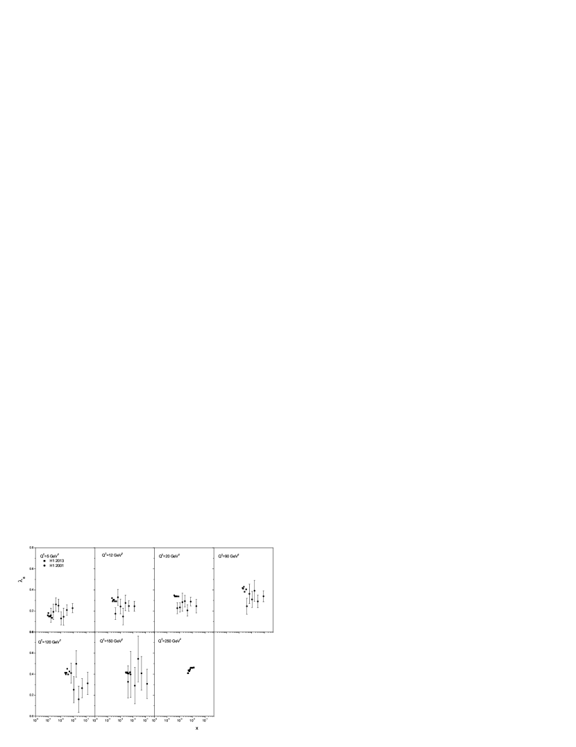
Figure 1: The singlet exponent $\lambda_{s}$ from H1 2013 data [17] compared with result H1 2001 [18-19] plotted against $x$ at $5\leq Q^{2}\leq 250~{}GeV^{2}$.

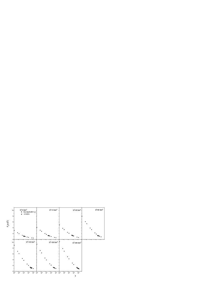
Figure 2: The proton structure functions $F_{2}(x,Q^{2})$ with respect to $<\lambda_{s}>$ compared with H1 data [17] as accompanied with total errors.

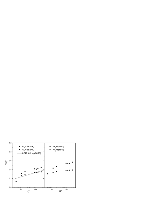
Figure 5: Averaged value of singlet and gluon exponents with respect to the critical point as functions of $Q^{2}$. The linear fit is a effective exponent to H1 and ZEUS data in Refs.21-22.

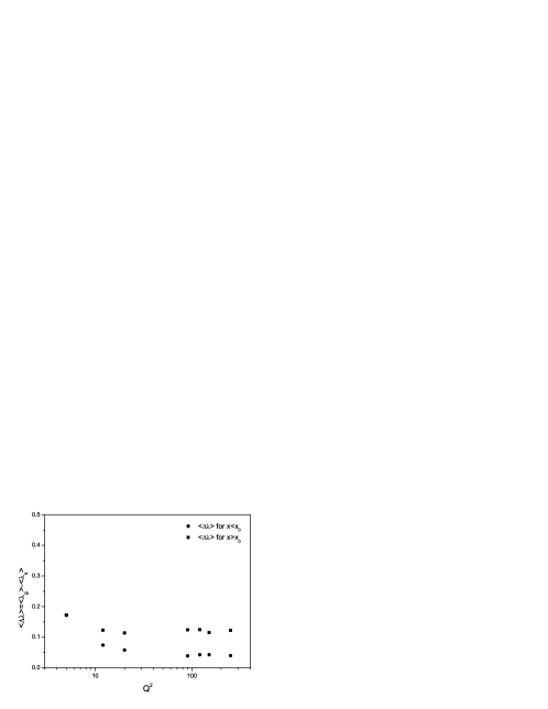
Figure 6: Different of singlet and gluon exponents as functions of $Q^{2}$.

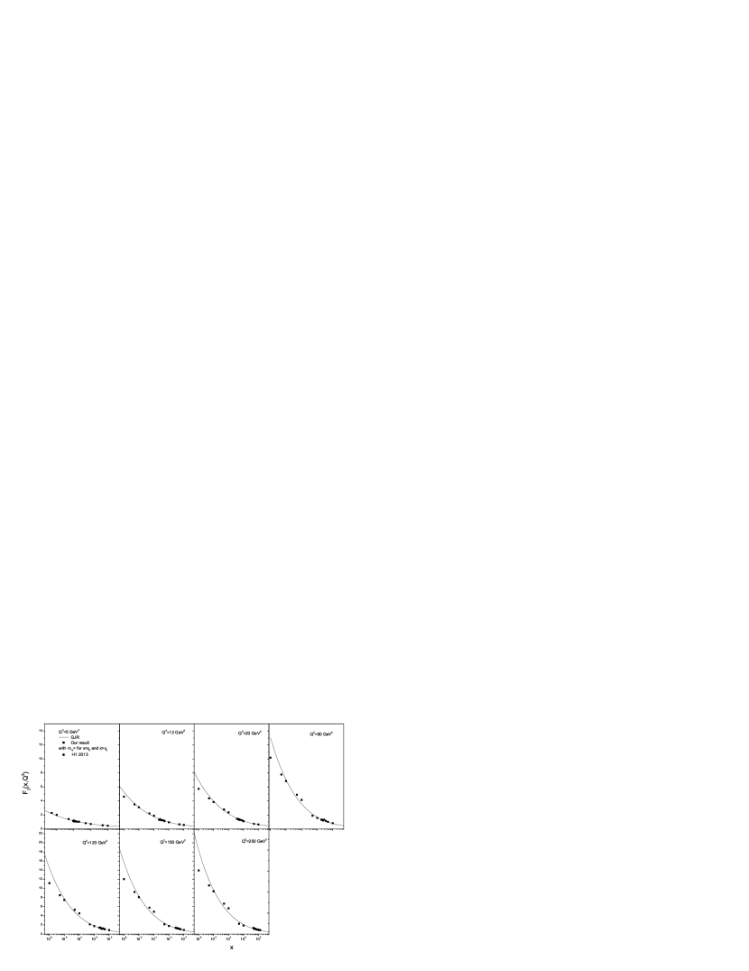
Figure 7: The determined values of the structure function $F_{2}(x,Q^{2})$ plotted as functions of $x$ with respect to the averaged exponent $<\lambda_{s}>$ for $x<x_{0}$ and $x>x_{0}$ compared with H1 data [17] and GJR parameterization [23].

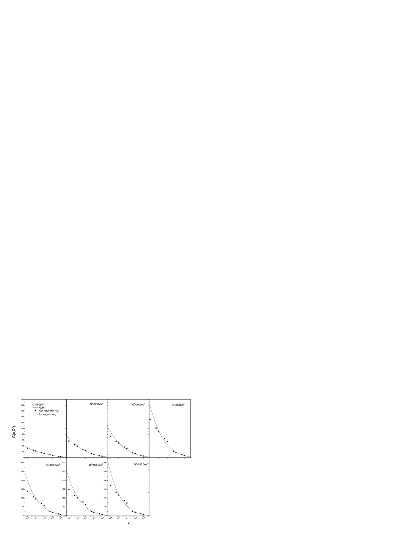
Figure 8: The gluon distribution against $x$ in a wide region of $Q^{2}$ values with respect to the averaged exponent $<\lambda_{g}>$ for $x<x_{0}$ and $x>x_{0}$ compared with GJR parameterization [23].

In order to show our results we computed the singlet and gluon distribution functions into the decoupled second order evolution equations. The initial conditions starts at $Q_{0}^{2}=1~{}GeV^{2}$ with $\alpha_{s}(1~{}GeV^{2})=0.49128$ and $\alpha_{s}(M_{z}^{2})=0.12018$ at NLO analysis [16]. The power law behavior of the distribution functions is considered in the decoupled DGLAP evolution equations. In principle if we take $F_{2}{\sim}x^{-\lambda_{s}}$ and $G{\sim}x^{-\lambda_{g}}$ then we might expect to determine $\lambda_{s}$ and $\lambda_{g}$. The behavior of exponent $\lambda_{s}$ at fixed $Q^{2}$ should be determined from Eq.9 by the proton structure function extracted from Ref.[17].
As can be seen in Fig.1, these derivatives are independent of $x$ when compared with H1 2001 data [18] within the experimental accuracy. In this figure we show $\lambda_{s}$ calculated as a function of $x$ for $5\leq Q^{2}\leq 250~{}GeV^{2}$ from H1 2013 data [17]. These result are consistent with other experimental data [19]. In order to test the validity of our obtained exponents, we introduce the averaged value $\lambda_{i},~{}(i=s~{}\mathrm{and}~{}g)$ (denoted in the following by $<...>$) in this research. In Fig.2 we show the NLO results for the proton structure function as a function of $<\lambda_{s}>$ as compared with H1 collaboration data [17].
It is tempting, however, to explore the possibility of obtaining approximate behavior of the exponents in the restricted color dipole model point (i.e., $x_{0}$). In Figs.3-4 the approximate behavior of the exponents are shown for $|\Delta{\lambda}_{i}|=\lambda_{i}-<\lambda_{i}>$. These data are obtained with respect to the decoupled DGLAP evolution equations in accordance with H1 data. We observed that $|\Delta{\lambda}|$ behaviors have a derivative at around a saddle point. Our fit to these results show that a minimal point (i.e., $x_{cut}$) is corresponding to the derivatives. As seen in these figures the saddle point is almost constant in a wide range of $Q^{2}$ values. This point approximately has the same value as observed for the color dipole model point (i.e. $x_{cut}\simeq x_{0}$).
Therefore we expect to have the intercepts for $x<x_{0}$ and $x>x_{0}$ where the averaged value is taken as a constant factor throughout the calculation. The results of the average to data are collected in Tables I and II for $x<x_{0}$ and $x>x_{0}$ respectively. In these tables a transition from the soft pomeron to the hard pomeron intercept for distribution functions observed as $Q^{2}$ increase. We observed that the low-$x$ behavior of the both gluon and sea quarks is controlled by the pomeron intercept.
In Fig.5 we show $<\lambda_{i}>$ obtained for singlet structure function and gluon distribution function at $x<x_{0}~{}\mathrm{and}~{}x>x_{0}$ and compared the singlet averaged value of $<\lambda_{s}>$ with $\lambda_{\mathrm{phn}}(Q^{2})$ parameterized in Ref.[21]. This phenomenologically exponent has been derived (Ref.[21]) for calculating the evolution of singlet density for combined HERA $e^{+}p$ DIS data [22] within the saturation model. With this method the low-$x$ behavior of the $F_{2}$ structure function has been shown that $F_{2}(x,Q^{2}){\sim}x^{-\lambda_{phn}(Q^{2})}$, where $\lambda_{phn}(Q^{2})$ can be parameterized as $\lambda_{phn}(Q^{2})=0.329+0.1\log(\frac{Q^{2}}{90})$.
In this figure (i.e. Fig.5) we observe that a linear behavior for exponents $<\lambda_{s}>$ at low-$Q^{2}$ values is dominant and this behavior is almost constant at high-$Q^{2}$ values. It is observed that the averaged exponent $<\lambda_{s}>$ shows almost similar behavior with $x<x_{0}~{}\mathrm{and}~{}x>x_{0}$ but in comparison with $\lambda_{phn}$ it shows that this behavior is nonlinear in wide range of $Q^{2}$ values. We also added results for the gluon exponent at low and high $Q^{2}$ values in the same figure. Similar remarks apply to the gluon exponent where the scale of the exponent has been fixed at a hard pomeron value.
One can see that exponents obtained for gluon distribution function from the decoupled evolution equations are larger than the singlet exponent, that is $\lambda_{g}>\lambda_{s}$. Indeed the steep behavior of the gluon generates a similar steep behavior of singlet at small-$x$ at NLO analysis where $\lambda_{s}=\lambda_{g}-\epsilon$. Furthermore, the exact solution of the decoupled evolution equations predicts that $\lambda_{s}$ and $\lambda_{g}$ are separated free parameters. This shows that the differences between these exponents are consistent with pQCD. In Fig.6 we compared $\Delta{\lambda}$ obtained using an averaged value between singlet and gluon exponents at $x<x_{0}~{}\mathrm{and}~{}x>x_{0}$. This $\Delta{\lambda}$ shows that a scaling behavior property is exhibited for $Q^{2}>5~{}GeV^{2}$. Note that this scaling for singlet and gluon exponents in Fig.5 is clear at moderate and high $Q^{2}$ values.
In Figures 7 and 8 we present the results for the proton structure function and the gluon distribution function at NLO analysis using the gluon and singlet exponents for $x<x_{0}~{}\mathrm{and}~{}x>x_{0}$ respectively. We compare our results with those obtained by GJR parameterizations [23] and H1 2013 experimental data [17]. The kinematical ranges for H1 2013 data are $10^{-7}<x<10^{-1}$ and $5\leq Q^{2}\leq 250~{}GeV^{2}$. These results in Fig.7 compared with H1 data and GJR parameterizations in a wide range of $x$ values based on averaged exponents for $x<x_{0}~{}\mathrm{and}~{}x>x_{0}$ . Also, in Fig.8, the gluon distribution behavior is compared with GJR parameterization with respect to the averaged exponent. These results indicate that our calculations, based on the averaged exponent for $x>x_{0}$ have of the same form behavior as the predicted by other results. But for $x<x_{0}$ the extrapolation to small $x$ has very large uncertainties when compared with GJR parameterization especially at large $Q^{2}$ values. This is because the averaged exponent behavior defined by our method (in Table I) is expected to hold in the small $x$ limit. However, due to the existence of absorptive corrections, this is not true pomeron intercept, but rather an effective one is necessary in this region [24]. The connection between the averaged value of exponent with effective exponent and color dipole model size is given in next sections.

V 5. Effective Exponents

Perturbative QCD predicts a strong power-law rise of the gluon and singlet distribution at low $x$. This behavior coming from resummation of large powers of $\alpha_{s}\ln 1/x$ where its achieved by the use of the $k_{T}$ factorization formalism. The small-$x$ resummation requires an all-order class of subleading corrections in order to lead to stable results. Authors in Ref.[25] discuss a framework to perform small-$x$ resummation for both parton evolution and partonic coefficient functions. In this paper a detailed analysis has been performed in order to find resummation of the DGLAP and BFKL evolution kernels at NNLO approximation.
In the leading log approximation this behavior leads to the unintegrated gluon distribution rising as a power of $x$. Which this result is given in terms of the BFKL evolution equation as $f(x,k_{T}^{2})\sim x^{-\lambda}$ [20]. The function $f(x,k_{T}^{2})$ is the unintergrated gluon distribution and related to the gluon distribution from the DGLAP evolution equation by integration over the transform momentum as $G(x,Q^{2})=\int^{Q^{2}}\frac{dk_{T}^{2}}{k_{T}^{2}}f(x,k_{T}^{2})$. One finds $\lambda=0.437$ where it is the so-called hard-Pomeron exponent. As an alternative to comparing with the experimental data an effective exponent $\lambda\simeq 0.3$ exhibited in Refs. [20-21]. The strong rise into the $k_{T}$ factorization formula is also true for the singlet structure function. The BFKL Pomeron does not depend on $Q^{2}$, however the effective Pomeron is $Q^{2}$-dependent when structure functions fitted to the experimental data at low values of $x$. This behavior can violate unitarity, so it has to be tamed by screening effects.
Indeed the nonlinear terms reduce the growth of singlet and gluon distributions at low-$x$. The transition point for gluon saturation is given by the saturation scale $Q_{s}^{2}=Q_{0}^{2}(\frac{x}{x_{0}})^{-\lambda}$ which is the $x$-dependent and this is an intrinsic characteristic of a dense gluon system. Here, we take into account the effects of kinematics which these are shown results a shift from the pomeron exponent to the effective exponent. This is related to fact that at low $x$ we needed to produce the color dipole model in the argument of the gluon distribution as it can be computed from the $k_{T}$ factorization formula [26]. We note that the nonlinear effects are small for $Q^{2}>Q_{s}^{2}$, but very strong for $Q^{2}<Q_{s}^{2}$ where leading to the saturation of the scattering amplitude. These two regions separated by the saturation line, $Q^{2}=Q^{2}_{s}$. When $x\rightarrow x_{0}$, we have $Q^{2}=Q^{2}_{s}\rightarrow 1$ and this line is independent of $\lambda$-exponent. With respect to the averaged values of $\lambda_{s}$ for $x<x_{0}~{}\mathrm{and}~{}x>x_{0}$, the relation $Q^{2}>Q_{s}^{2}$ is satisfied always when we used the HERA kinematical region for $5\leq Q^{2}\leq 250~{}GeV^{2}$ and $10^{-6}\leq x\leq 10^{-2}$. However we do not observe the nonlinear behavior by these exponents.
In Tables III and IV, we show some of parameters determined for the saturation behavior of the singlet structure function. These saturation parameters are obtained at $Q^{2}=5~{}GeV^{2}$ and $250~{}GeV^{2}$ respectively. We note that the averaged exponent $<\lambda_{s}>$ is taken into account from Tables I and II. In Tables III and IV, the saturation scale is defined in the form $R_{0}^{2}(x)=\frac{1}{Q_{0}^{2}}(\frac{x}{x_{0}})^{\lambda}$ where $Q_{0}^{2}=1~{}GeV^{2}$. Indeed $R_{0}(x)$ decreases when $x\rightarrow 0$. Here the dimensionless variable $\tau$ is taken with a simplest form $\tau=Q^{2}R_{0}^{2}(x)$ throughout the method [20].
The saturation radius is defined by $r_{s}=2R_{0}(x)$ because its decrease with decreasing $x$. Indeed if $r<r_{s}(x)$ the dipole cross section increase as $x$ decreases. We note that the variable $r$ denotes the separation between the quark and antiquark in color dipole model. This transverse dimension of the $q\overline{q}$ pair is small when the condition $r<\frac{1}{Q}$ is fulfilled and large when $r>\frac{1}{Q}$. In Fig.9 we analyse the ratio of the dipole cross section, $\sigma/\sigma_{0}$, for different dimensionless variable $\tau$. As expected the saturation lies in the small-$r$ region when compared the region $x<x_{0}$ with $x>x_{0}$.
To better illustrate nonlinear effects at $Q^{2}<Q^{2}_{s}$, we average over the exponents for $5\leq Q^{2}\leq 250~{}GeV^{2}$ presented in Tables I and II. As optimal values of parameters $\lambda_{s}$ and $\lambda_{g}$ we take $\lambda_{ave}$ over the two different regimes as we have

$$<\lambda_{s}>=0.295~{}~{}\mathrm{for}~{}~{}x<x_{0}~{}~{}~{}\mathrm{and}~{}~{}~{}0.358~{}~{}\mathrm{for}~{}~{}x>x_{0},$$

$$<\lambda_{g}>=0.362~{}~{}\mathrm{for}~{}~{}x<x_{0}~{}~{}~{}\mathrm{and}~{}~{}~{}0.485~{}~{}\mathrm{for}~{}~{}x>x_{0}.$$

Therefore the averaged value to all exponents has the effective constraint as we obtained the following effective exponents and taking all into account.

$$\lambda^{eff}_{s}=0.327~{}\mathrm{and}~{}\lambda^{eff}_{g}=0.424.$$ (19)

One can see that the averaged exponents obtained for singlet and gluon distributions are closer to those defined by color dipole model and hard-pomeron exponents. In Ref.[21], authors have shown that the inclusive DIS value of singlet exponent is defined as $\lambda_{inc}=0.298\pm 0.011$, for combined HERA DIS data where errors are purely statistical. This parameter is defined to be $0.29$ in GBW model [20] and it is an effective intercept in BFKL kernel. Also $\lambda_{g}$ is comparable with the so-called hard Pomeron intercept [27].
Now the saturation condition $Q^{2}<Q_{s}^{2}$ is visible for low $x$ values at low and moderate $Q^{2}$ values. As illustrated in Fig.10 the transition occurs for decreasing transverse sizes at very low $x$ values. We observe a continuous behavior of the dipole cross section saturation towards small-$r$. The saturation form of the ratio $\sigma/\sigma_{0}$ is modified in comparison with Fig.9 based on the effective exponents. Therefore these exponents (i.e. Eq.19) guarantees consistency low $x-Q^{2}$ behavior with saturation effects. The proton structure function behavior with respect to this effective exponent will study in next section.

VI 6. The behavior of the structure function

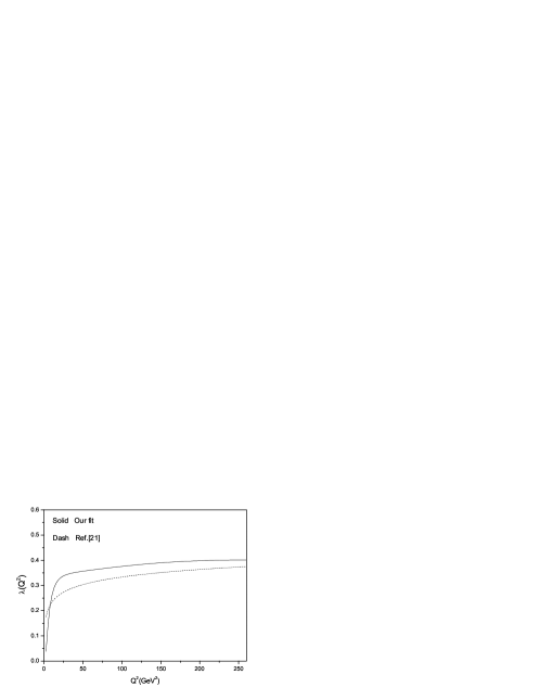
Figure 12: Effective exponent $\lambda(Q^{2})$ from averaged exponents compared with Ref.[21].

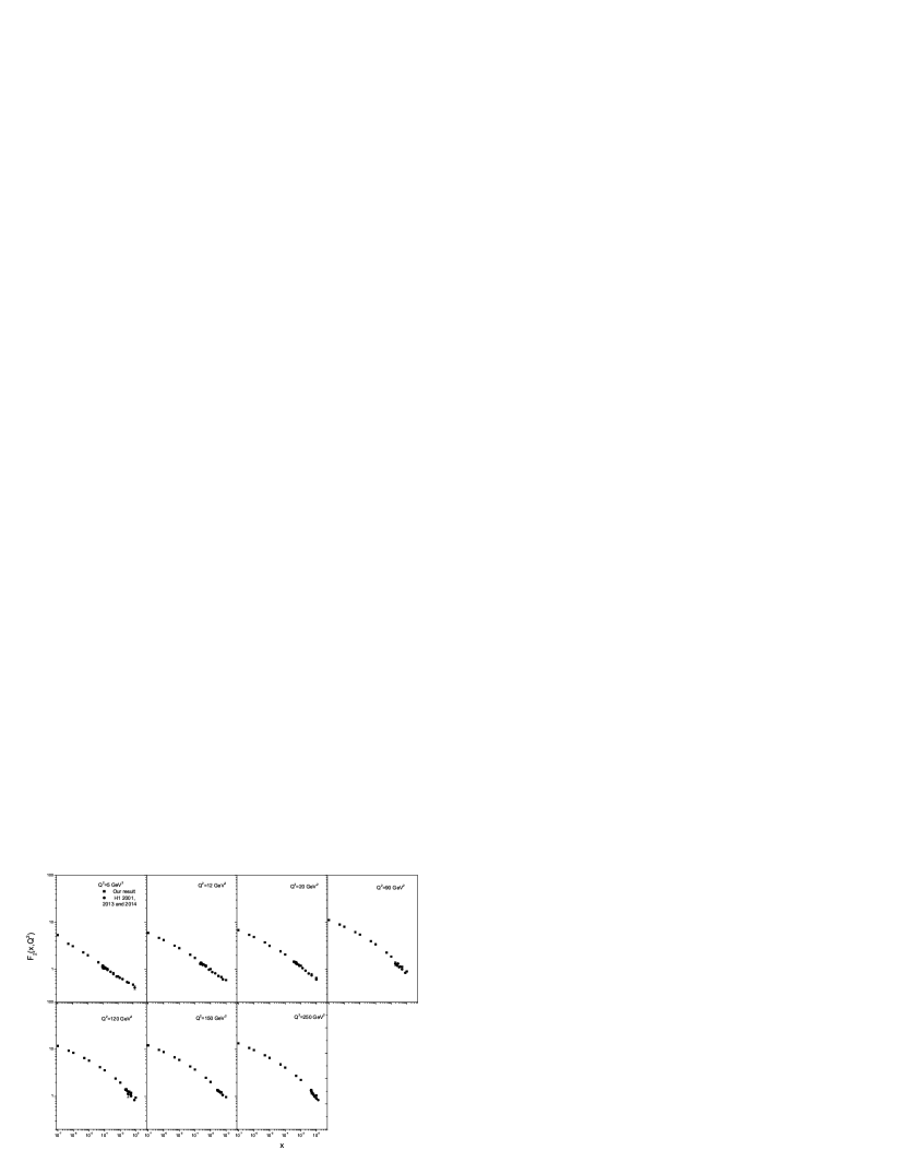
Figure 13: The proton structure function obtained by effective exponent $\lambda(Q^{2})$ compared with H1 data [17-19,22].

In order to show the saturation effects at low values of $x$, we computed the proton structure function by the effective exponent obtained in Eq.19. In Fig.11 the $F_{2}$ structure function is plotted as a function of $x$ in bins of $Q^{2}$ at NLO analysis. We compare our results with H1 experimental data [17-19,22]. The agreement between the experimental data and our calculation at moderate-$Q^{2}$ values is good, as the exponent value $\lambda\sim 0.33$ is served for inclusive DIS and other methods. At low and high-$Q^{2}$ values we observed an overall shift between the H1 data and the predictions. This behavior can be resolved with an adjustment of lower and higher exponents than one obtained for decoupled distributions respectively.
Notice that this behavior for the effective exponent is closer than to the linear behavior with $\log Q^{2}$ as given in Ref.21. Indeed this behavior depends on fixed effective exponent which we constrain analyzing for $Q_{s}$. In Fig.11 this prediction obtained at very low-$x$ values as the exponent is fixed in accordance with an effective intercept. It is tempting, however, to explore the possibility of obtaining an effective exponent dependent on $Q^{2}$ in the restricted domain of all $Q^{2}$ values at least. In Fig.12, $\lambda(Q^{2})$ depicted and compared with the linear dependence on $\log Q^{2}$ in Ref.[21]. To better illustrate our calculations at all $Q^{2}$ values, we used therefore effective exponent in the form of $\lambda(Q^{2})$ in Fig.13. This figure indicate that the obtained results from present analysis based on $\lambda(Q^{2})$ are in good agreements with H1 data for the proton structure function. These results have been presented as a function of $x$ (both for large and small $x$ ) at $5\leq Q^{2}\leq 250~{}GeV^{2}$. In transition to the saturation model for low $Q^{2}$, one should take into account the quark mass, when we replace $x{\rightarrow}(1+\frac{4m_{c}^{2}}{Q^{2}})x$ in decoupled evolution equations [28]. Indeed one can modify $\tau=\frac{Q^{2}}{Q^{2}_{0}}(\frac{x}{x_{0}})^{\lambda}$ to take into account $m_{c}\simeq 1.3~{}GeV^{2}$ and introduce scaling $\tau_{c}=(1+\frac{4m_{c}^{2}}{Q^{2}})\frac{Q^{2}}{Q^{2}_{0}}(\frac{x}{x_{0}})^{\lambda}$ [29]. However the transition to the low and high $Q^{2}$ values is related to the regions that $\lambda_{s}<\lambda^{eff}_{s}(\simeq 0.33)$ and $\lambda_{s}>\lambda^{eff}_{s}(\simeq 0.33)$ respectively, as we observed that the effective exponent is not a linear function into $\log Q^{2}$. It has the nonlinear behavior with respect to the low and high $Q^{2}$ values.

VII 7. Conclusion

We presented the high-order decoupled analytical evolution equations for distribution functions, arising from the coupled DGLAP evolution equations. The Laplace transform technique used for the decoupled proton structure function and gluon distribution function evolution equations. Two homogeneous second-order differential evolution equations are obtained and extended to the nonlinear behavior at low-$x$ region. The next-to-leading -order analysis compared with H1 data with the averaged value of exponent $\lambda_{s}$. The averaged value of exponent $\lambda_{s}$ has different behavior when the color dipole model is considered around the $x_{0}$ value. The different between the gluon and singlet exponents considered at low-$x$ values and shown that they have the nonlinear behavior into $\log Q^{2}$. The dipole cross section considered for nonlinear behavior at $Q^{2}<Q^{2}_{s}$, as this behavior is very important for shown that the effective exponent with exact value is necessary for saturation effect. This effective exponent is basically the value of $\simeq 0.33$ as reported in the literature. The proton structure function determined and compared with respect to this effective exponent for $10^{-7}\leq x\leq 10^{-2}$ and $5\leq Q^{2}\leq 250~{}GeV^{2}$.

VIII References

1. V. N. Gribov and L. N. Lipatov, Sov. J. Nucl. Phys. 15 (1972) 438; G. Altarelli and G. Parisi, Nucl. Phys. B126 (1977) 298; Y. L. Dokshitzer, Sov. Phys. JETP46 (1977)641.
2. M.Klein, Ann.Phys.528(2016)138.
3. P.Kostka et.al., Pos DIS2013 (2013)256; L.Han et.al., Phys.Lett.B771(2017)106; L.Han et.al., Phys.Lett.B768(2017)241; Yao-Bei Liu, Nucl.Phys.B923(2017)312.
4. E.Gotsman et.al., Nucl.Phys.B539 (1999)535; K.J.Eskola et.al., Nucl.Phys.B660 (2003)211.
5. L.V.Gribov, E.M.Levin and M.G.Ryskin, Phys.Rep.100, (1983)1; A.H.Mueller and J.Qiu, Nucl.Phys.B268 (1986)427.
6. B.Rezaei and G.R.Boroun, Phys.Letts.B692(2010)247; G.R.Boroun, Eur.Phys.J.A42(2009)251; G.R.Boroun, Eur.Phys.J.A43(2010)335.
7. P.Phukan et.al., arXiv:hep-ph/1705.06092; M.Lalung et.al., arXiv:hep-ph/1702.05291; M.Devee and J.K.sarma, Eur.Phys.J.C74(2014)2751; M.Devee and J.K.sarma, Nucl.Phys.B885(2014)571.
8. G.R.Boroun and S.Zarrin, Eur.Phys.J.Plus 128(2013)119; B.Rezaei and G.R.Boroun, Eur. Phys. J. C73(2013)2412; G.R.Boroun and B.Rezaei, Eur.Phys.J.C72(2012)2221.
9. Martin M.Block et al., Eur.Phys.J.C69(2010)425; Phys.Rev.D84(2011)094010; Phys.Rev.D88(2013)014006.
10. F.Taghavi-Shahri et al., Eur.Phys.J. C71 (2011) 1590.
11.S.Shoeibi et al., Phys.Rev. D97 (2018) 074013.
12. H.Khanpour, A.Mirjalili and S.Atashbar Tehrani, Phys.Rev.C95(2017)035201.
13. A. Vogt, S. Moch and J.A.M. Vermaseren, Nucl.Phys.B691(2004)129.
14. C.D. White and R.S. Thorne, Eur.Phys.J.C45 (2006)179.
15. B.G. Shaikhatdenov, A.V. Kotikov, V.G. Krivokhizhin, G. Parente, Phys. Rev. D 81(2010) 034008.
16. A.D.Martin, et al., Eur.Phys.J.C63 (2009)189.
17. V. Andreev et al. (H1 Collaboration), Eur. Phys. J. C74 (2014) 2814.
18. C.Adloff et al. (H1 Collaboration), Eur. Phys. J. C21 (2001) 33.
19. C.Adloff et al. (H1 Collaboration), Phys.Lett.B520 (2001) 183.
20. K.Golec-Biernat and M.Wuesthoff, Phys.Rev.D59 (1999) 014017; K.Golec-Biernat, Acta.Phys.Polon.B33 (2002) 2771.
21. M. Praszalowicz and T.Stebel, JHEP 03 (2013) 090; T.Stebel, Phys. Rev. D88 (2013) 014026.
22. F.D.Aaron et al. (H1 and ZEUS Collaboration), JHEP1001 (2010) 109; Eur.Phys.J.C 63 (2009) 625; Eur.Phys.J.C 64 (2009) 561.
23. M.Gluk, P.Jimenez-Delgado and E.Reya, Eur.Phys.J.C53(2008)355.
24.A.Donnachie and P.V.Landshoff, Phys.Lett.B550(2002)160; G.R.Boroun and B.Rezaei, Phys.Atom.Nucl.71(2008)1077.
25. M.Bonvini et.al., Eur.Phys.J.C76(2016)597.
26. V.P.Goncalves and M.V.T.Machado, Phys.Rev.Lett.91 (2003) 202002.
27. L. Motyka et al., arXiv:0809.4191v1 (2008); H.Kowalski et al., Eur.Phys.J.C77(2017)777.
28. Z.Jalilian and G.R. Boroun, Phys.Lett. B773(2017)455.
29. E.Avsar and G.Gustafson, JHEP0704 (2007) 067.

Table 1: Averaged value of exponents for $Q^{2}$ values at $x<x_{0}$.

$Q^{2}(GeV^{2})$	$<\lambda_{s}>$	$<\lambda_{g}>$
5	0.135	0.307
12	0.262	0.336
20	0.295	0.353
90	0.337	0.376
120	0.342	0.385
150	0.344	0.387
250	0.351	0.391

Table 2: The same as Table I but for $x>x_{0}$.

$Q^{2}(GeV^{2})$	$<\lambda_{s}>$	$<\lambda_{g}>$
5	0.135	0.307
12	0.312	0.435
20	0.356	0.470
90	0.419	0.543
120	0.411	0.536
150	0.425	0.540
250	0.445	0.567

Figure 3: The singlet intercept behavior obtained for different energies as functions of $x$. Solid curve is our fit to all data.

Figure 4: As in Fig.3 but for the gluon exponent behavior.

Figure 9: The ratio of the dipole cross section with respect to the averaged exponent $<\lambda_{s}>$ for $x<x_{0}~{}\mathrm{and}~{}x>x_{0}$ at different values of $\tau$.

Figure 10: The ratio of the dipole cross section with respect to the effective exponent $\lambda_{s}^{eff}=0.327$ for different values of $x$.

Figure 11: Comparison of the proton structure function obtained from the decoupled evolution equation with the effective exponent with the H1 data collected since 2001 until 2014 [17-19,22].

Table 3: Parameters determined at $Q^{2}=5~{}GeV^{2}$ for regions $x<x_{0}$ and $x>x_{0}$.

$x$	$Q_{s}^{2}(GeV^{2})|_{x<x_{0}}$	$Q_{s}^{2}(GeV^{2})|_{x>x_{0}}$	$R_{0}^{2}(GeV^{-2})|_{x<x_{0}}$	$R_{0}^{2}(GeV^{-2})|_{x>x_{0}}$
1E-6	2.160	—–	0.463	—–
5E-6	1.738	—–	0.575	—–
1E-5	1.583	—–	0.632	—–
5E-5	1.274	—–	0.785	—–
1E-4	1.160	—–	0.862	—–
5E-4	—–	0.934	—–	1.071
1E-3	—–	0.850	—–	1.177
5E-3	—–	0.684	—–	1.462
1E-2	—–	0.623	—–	1.605

Table 4: The same as Table III but for $Q^{2}=250~{}GeV^{2}$.

$x$	$Q_{s}^{2}(GeV^{2})|_{x<x_{0}}$	$Q_{s}^{2}(GeV^{2})|_{x>x_{0}}$	$R_{0}^{2}(GeV^{-2})|_{x<x_{0}}$	$R_{0}^{2}(GeV^{-2})|_{x>x_{0}}$
1E-6	7.404	—–	0.135	—–
5E-6	4.208	—–	0.238	—–
1E-5	3.300	—–	0.303	—–
5E-5	1.876	—–	0.533	—–
1E-4	1.470	—–	0.680	—–
5E-4	—–	0.800	—–	1.255
1E-3	—–	0.585	—–	1.709
5E-3	—–	0.286	—–	3.497
1E-2	—–	0.210	—–	4.761