A Zone of Avoidance catalogue of 2MASS bright galaxies. I. Sample description and analysis

Abstract

We present a homogeneous 2MASS bright galaxy catalogue at low Galactic latitudes ($|b|\leq 10\aas@@fstack{\circ}0$, called Zone of Avoidance) which is complete to a Galactic extinction-corrected magnitude of $K^{\rm o}_{\rm s}$ $\leq 11\aas@@fstack{m}25$. It also includes galaxies in regions of high foreground extinctions ($E(B-V)$$>0\aas@@fstack{m}95$) situated at higher latitudes. This catalogue forms the basis of studies of large-scale structures, flow fields and extinction across the ZoA and complements the ongoing 2MASS Redshift and Tully-Fisher surveys. It comprises 3763 galaxies, 70% of which have at least one radial velocity measurement in the literature. The catalogue is complete up to star density levels of $\log N_{*}/{\rm deg}^{2}<4.5$ and at least for $A_{\rm K}<0\aas@@fstack{m}6$ and likely as high as $A_{\rm K}=2\aas@@fstack{m}0$. Thus the ZoA in terms of bright NIR galaxies covers only $2.5-4$% of the whole sky. We use a diameter-dependent extinction correction to compare our sample with an unobscured, high-latitude sample. While the correction to the $K_{\rm s}$-band magnitude is sufficient, the corrected diameters are too small by about $4^{\prime\prime}$ on average. The omission of applying such a diameter-dependent extinction correction may lead to a biased flow field even at intermediate extinction values as found in the 2MRS survey. A slight dependence of galaxy colour with stellar density indicates that unsubtracted foreground stars make galaxies appear bluer. Furthermore, far-infrared sources in the DIRBE/IRAS extinction maps that were not removed at low latitudes affect the foreground extinction corrections of three galaxies and may weakly affect a further estimated $\lower 1.99997pt\hbox{$\buildrel<\over{\sim}$}20$% of our galaxies.

1 Introduction

Truly all-sky galaxy samples are difficult to acquire because of the so-called Zone of Avoidance (hereafter ZoA). In the ZoA, Galactic dust extinction as well as star crowding severely hamper not only the identification of galaxies (where different wavelengths are affected by different biases, e.g., Kraan-Korteweg & Lahav 2000 and references therein) but also subsequent follow-up observations.

While all-sky imaging surveys exist, like photographic plate surveys in the optical such as the Palomar Observatory Sky Survey (POSS) and the UK-Schmidt telescope (SERC) surveys (now available in digitised format at DSS and SuperCOSMOS), and more recent CCD-based surveys in the NIR such as 2MASS (Two Micron All Sky Survey; Skrutskie et al. 2006), many other surveys cover only one hemisphere (at least in one passband), e.g., DENIS (DEep Near-Infrared southern sky Survey; Epchtein et al. 1997), VHS (VISTA Hemisphere Survey; McMahon et al. 2013), HIPASS (H I Parkes All-Sky Survey; Meyer et al. 2004), the DESI Legacy Imaging Surveys (Dey et al. 2018), and the upcoming LSST (Large Synoptic Survey Telescope, LSST Science Collaboration et al. 2009) survey. For extragalactic surveys and cosmic flow field analyses, the objective is the identification of galaxies, who can then be targeted for redshift measurements. Thus not only the distinction between extended sources and point sources but also between Galactic and extragalactic extended sources is tantamount. Automated galaxy detection algorithms work well at high latitudes where the spatial density of foreground stars is low and Galactic extended sources scarce, but they are far inferior to the human eye in the crowded areas of the Galactic Plane. Though such by-eye searches of the ZoA were done extensively using photographic plates (e.g., Kraan-Korteweg 2000, Woudt & Kraan-Korteweg 2001 in the south and Saito et al. 1991 in the north), the modern CCD-based, high-resolution surveys, like the UKIDSS GPS (Galactic Plane Survey; Lucas et al. 2008), the Vista VVV (VISTA Variables in the Vía Lactea; Minniti et al. 2010) and the DECam Plane Survey (Schlafly et al., 2018), have a depth and spatial resolution that renders such searches impossible within a reasonable time span.

Furthermore, for a 3-dimensional (3D) view of the sky, spectroscopic surveys are required which usually depend on a galaxy sample as input and are thus, even when based on an all-sky imaging survey, usually restricted to higher Galactic latitudes (e.g., 2MRS: the 2MASS Redshift Survey, Huchra et al. 2012; the 6dF Galaxy Survey, Jones et al. 2009; the Sloan Digital Sky Survey SDSS, York et al. 2000). Only so-called blind H I surveys with their great advantage of a 3D view of observed areas of the sky cover the ZoA as well (e.g., HIPASS, Meyer et al. 2004; HIJASS: the H I Jodrell All Sky Survey, Lang et al. 2003; EBHIS: the Effelsberg Bonn H I Survey, Kerp et al. 2011). Disadvantages of surveys in H I are the intrinsical weakness of the 21 cm line emission, which leads to a restricted coverage in redshift out to which galaxies can be detected, as well as the paucity of H I in certain types of galaxies, in particular of elliptical galaxies and early-type spirals that often define the centres of massive clusters. The advantages are that galaxies can be detected independent of foreground extinction and star crowding (though their detection is affected by the presence of radio continuum sources which are more frequent in the Galactic Plane, Staveley-Smith et al. 2016). Thus, blind H I surveys of the ZoA have been the tool of choice in mapping large-scale structures in this area (e.g., HIZOA: the H I Zone of Avoidance survey, Staveley-Smith et al. 2016; HIZOA-NE: the HIZOA Northern Extension survey, Donley et al. 2005; ALFAZOA: the Arecibo L-band Feed Array Zone of Avoidance Survey, Henning et al. 2010; EZOA: the EBHIS Zone of Avoidance survey, Schröder et al., in prep.).

Truly all-sky galaxy samples that are homogeneous are therefore difficult to compile but they are important to arrive at a complete and unbiased 3D map of the local universe required to explain the dynamics in the local universe (e.g., Qin et al. 2018 using 2MTF and 6dFGSv, Courtois et al. 2017 using CosmicFlows3, Lavaux & Jasche 2016 using 2M++, Erdoǧdu et al. 2006 using 2MRS) including structures such as the Great Attractor (Dressler et al., 1987), the Perseus Pisces Complex (Giovanelli & Haynes, 1982) or the Local Void (Tully et al., 2008). Even though the gap due to the ZoA is considerably smaller in the NIR than in the optical, the incompleteness in the 3D galaxy mass distribution due to the ZoA still leads to new discoveries (e.g., the Vela Supercluster, Kraan-Korteweg et al. 2017, Sorce et al. 2017; a rich cluster in the Perseus-Pisces filament, Ramatsoku et al. 2016) and still has an impact on the studies of the cosmic flow fields where controversies remain in modelling the dipole of the cosmic microwave background (e.g., Kraan-Korteweg & Lahav 2000, Loeb & Narayan 2008). For more information, see our Paper II (Kraan-Korteweg et al., 2018).

Another advantage of defining a homogeneous galaxy sample that includes the high extinction areas of the ZoA is that it allows the study of systematic effects which are caused by an incomplete understanding of the impact of extinction on galaxy sample selections that are based on magnitudes or size. Even at higher Galactic latitudes ($|b|>10\degr$) there are areas of higher extinction on the sky (e.g., the Orion Nebula or the Taurus Molecular Cloud) where incompletely corrected galaxy magnitudes could lead to systematic biases in an all-sky analysis (see our discussion on Galactic extinction corrections in Sec. 3).

We therefore compiled a magnitude-limited sample of 2MASS galaxies in the ZoA to contribute to a homogeneous ‘whole-sky’ 2MRS for large-scale structure studies in the nearby Universe, as well as to the ‘whole-sky’ 2MASS Tully Fisher Relation Survey (2MTF; e.g., Masters et al. 2014) of inclined spiral galaxies to study cosmic flow fields. Although both these major surveys intend to map the full three-dimensional distribution of galaxies in the nearby universe they have excluded the inner part of the ZoA ($|b|<5\degr$), and are not fully complete for its outer part ($5<|b|<10\degr$). Both are based on the 2MASS extended source catalogue (2MASX; Jarrett 2004) and have a $K_{\rm s}$-band magnitude completeness limit of $11\aas@@fstack{m}75$ and $11\aas@@fstack{m}25$, respectively. Though the 2MASX catalogue itself includes the ZoA, its reliability drops off quickly at low latitudes ($|b|<10\degr$; Jarrett et al. 2000, Huchra et al. 2012).

Contrary to the 2MRS magnitude limit of $K^{\rm o}_{\rm s}$ $<11\aas@@fstack{m}75$, we adopted a brighter limit of $K^{\rm o}_{\rm s}$ $<11\aas@@fstack{m}25$, which is the same as the limit of the first 2MRS data release (Huchra et al., 2005) as well as that of the 2MTF survey. At this extinction-corrected magnitude limit the 2MASX completeness level remains fairly constant across the ZoA (Huchra et al., 2005) apart from the Galactic Bulge. The completeness would drop substantially towards lower latitudes, however, if the extinction-corrected magnitude limit is lowered to include fainter ZoA objects, due to the steep increase in the number of faint foreground stars and the related rise in sky background close to the Galactic Plane (Jarrett et al., 2000). Furthermore, deep in the ZoA the $K_{\rm s}$-band extinction corrections can reach values of up to 1 magnitude, which implies that the apparent uncorrected magnitudes are quite faint which will affect both the accuracy of their photometry as well as their morphological classification. The $K^{\rm o}_{\rm s}$ $=11\aas@@fstack{m}25$ limit corresponds to a $B$-band limit of $14\aas@@fstack{m}75$ for an average spiral galaxy colour of $B-K=3\aas@@fstack{m}5$ (Jarrett et al., 2003; Jarrett, 2000), and is thus comparable to the completeness limit of most optically selected nearby galaxies whole-sky surveys (Kraan-Korteweg & Lahav, 2000).

Originally, our intention was to observe 2MASS galaxies in the northern ZoA that had no prior redshifts in the 21 cm line, using the 100 m class Nançay Radio Telescope (NRT). So far no systematic H I surveys of galaxies have been conducted over the northern ZoA, unlike in the south where pointed as well as blind H I surveys were made using the Parkes radio telescope (e.g., Kraan-Korteweg et al. 2002; Donley et al. 2005; Schröder et al. 2009; Staveley-Smith et al. 2016) or at medium declinations using the Arecibo telescope (e.g., Pantoja et al. 1994, Pantoja et al. 1997). And with an interstellar extinction in the $K_{\rm s}$-band ($\lambda\,2.2\,\mu$m) 11 times smaller than in the $B$-band, absorption remains relatively modest for galaxies in this passband over most of the northern ZoA, despite many being invisible on optical Palomar Sky Survey (DSS, Digital Sky Survey) images, while confusion due to star-crowding in the NIR is minimal for most of the northern ZoA. We thus started with a list of about 1100 2MASX objects compiled by J. Huchra (priv. comm.) mostly at $|b|<5\degr$ and $\delta>-40\degr$ (so as to be observable with the NRT), then formalised the selection criteria to include all objects from the 2MASS NIR extended objects catalogue (Jarrett et al., 2000) of the 2MASS survey at $|b|<10\degr$. For completeness reasons and to finally have a homogeneous all-ZoA (and thus all-sky) galaxy sample, we extended our sample to cover the southern ZoA as well as high-latitude high extinction areas to fully complement the 2MRS.

This paper is the first of a series. A pilot project based on 197 2MASX ZoA galaxies was presented by van Driel et al. (2009). In Paper II (Kraan-Korteweg et al., 2018) – (Kraan-Korteweg et al. 2018) we present the results of our NRT H I survey of a thousand 2MASX ZoA galaxies, and Paper III (Schröder et al., in prep.) will address the Galactic foreground extinction in the ZoA. Further publications will include observations at more southern declinations using the Parkes radio telescope, H I observations of galaxies with redshifts (mainly in the optical, but also of those galaxies with lower grade H I spectra) that are eligible for the TF analysis, as well as the flow-field analysis using the NIR Tully-Fisher relation.

This paper is structured as follows: in Sec. 2, our sample selection and extraction is described and in Sec. 3 details and limitations of the selection criteria are discussed. Sec. 4 presents the catalogue, and its properties are discussed in Sec. 5. Section 6 gives the summary and discussion. A supplementary catalogue of ZoA galaxies which need to be included in a sample when optimised extinction corrections are applied is presented in the appendix.

2 The sample

As mentioned in the introduction, our foremost aim is to complement the 2MRS and 2MTF efforts by obtaining redshifts of bright galaxies in the ZoA, that is, in the latitude range not covered by the 2MRS. The 2MRS sample selection criteria are:

1. $K^{\rm o}_{\rm s}$ $\leq 11\aas@@fstack{m}75$;

2. $E(B-V)$ $<1\aas@@fstack{m}0$;

3. also detected at $H$-band;

4. $|b|>5\aas@@fstack{\circ}0$ for $30\degr<l<330\degr$; $|b|>8\aas@@fstack{\circ}0$ otherwise.

We selected our sample using $K_{\rm s}$-band magnitudes corrected for Galactic extinction, $K^{\rm o}_{\rm s}$. To be as close as possible to the 2MRS magnitude-selection criterion, we extracted the $E(B-V)$ Galactic extinction values directly from the DIRBE/IRAS maps by Schlegel et al. (1998, hereafter SFD98) and did not correct for the factor of 0.86 applied by Schlafly & Finkbeiner (2011, hereafter SF11).

We defined two samples of galaxy candidates from the 2MASX catalogue: the main sample, which we will refer to as the ZOA sample, and the complementary EBV sample at higher latitudes. Their selection criteria are as follows:

Both samples: unlike the 2MRS, we did not require detection in the $H$-band but chose a slightly brighter magnitude limit than the 2MRS, i.e., $K^{\rm o}_{\rm s}$$\leq 11\aas@@fstack{m}25$.

ZOA sample: objects at $|b|\leq 10\aas@@fstack{\circ}0$ at all Galactic longitudes;

EBV sample: all objects at $|b|>10\aas@@fstack{\circ}0$ with $E(B-V)$$>0\aas@@fstack{m}95$. The overlap between our $E(B-V)$ limit and that of the 2MRS (i.e., $1\aas@@fstack{m}0$) covers any small variations in the determination of $E(B-V)$;

Galaxy candidates: both samples (particularly at high extinctions and high star-density regions) are contaminated with Galactic Nebulae and blended stars. We therefore visually inspected all 2MASX objects to decide whether they are likely galaxies or not (for further details, see Sec. 2.1).

To search for radial velocity information, we cross-correlated both our samples with the 2MRS catalogue as well as with the NASA/IPAC Extragalactic Database (NED) and the HyperLeda database.

2.1 Sample extraction

Table 1: Extinction correction factors in the NIR

Passband	$\lambda$	$A_{\lambda}$ / $A_{\rm B}$	Reference
	($\mu$m)
$J$	$\phantom{1}1.25$	0.21	Fitzpatrick 1999
$H$	$\phantom{1}1.65$	0.13	Fitzpatrick 1999
$K_{\rm s}$	$\phantom{1}2.15$	0.09	Fitzpatrick 1999
$w1$	$\phantom{1}3.4$	0.057	Schlafly et al. 2016
$w2$	$\phantom{1}4.6$	0.045	Schlafly et al. 2016
$w3$	$12.0$	0.086	Davenport et al. 2014

Our catalogue is based on the 2MASX catalogue. For the ZOA sample, we first downloaded all sources with $|b|\leq 10\aas@@fstack{\circ}0$, using the default SQL constraints given in the webform, i.e., deselecting sources with contamination and confusion flags, which are usually marked as “junk” (cc_flg= ‘$a$’ for known artefacts and ‘$z$’ for small detections in close proximity to large galaxies). This resulted in 146 174 sources. We extracted extinction values for each source using the SFD98 maps supplied through their webpage and the dust_getval script, setting the interp parameter to ‘y’. We determined the extinction correction in the $K_{\rm s}$-band using $R_{\rm B}=A_{\rm B}$/$E(B-V)$ = 4.14 and the conversion $A_{\rm K}=0.09A_{\rm B}$ (Fitzpatrick 1999). Table 1 lists the extinction correction factors compared to the $B$-band value for all passbands used in this publication. We applied this $K_{\rm s}$-band extinction correction to the 20 mag arcsec^-2 isophotal magnitude, $K_{20}$, and cut the list at the corrected $K^{\rm o}_{\rm s}$ $\leq 11\aas@@fstack{m}25$, which resulted in 6913 sources.

For the higher-latitude EBV sample, we first extracted all 2MASX-sources at $|b|>10\aas@@fstack{\circ}0$, obtained their $E(B-V)$ values and applied a cut at $E(B-V)$$\geq 0\aas@@fstack{m}95$, leading to 4248 sources. Applying the $K^{\rm o}_{\rm s}$ $\leq 11\aas@@fstack{m}25$ limit results in 502 sources.

The 2MASX sources in the ZoA are not all extragalactic in nature but also comprise various kinds of Galactic sources, including multiple stars and small stars on diffraction spikes (Jarrett et al., 2000). Although the 2MASX catalogue provides a visual verification score ‘vc’ which separates truly extended sources from stars and artefacts, it does not separate out candidate galaxies from Galactic sources, and we visually inspected all 7415 sources. Even to the human eye, galaxy classification in the ZoA is not straight forward. A major problem are the ambient high stellar densities: Superimposed stars hinder the identification of a halo-like disc structure around the core region, while the ubiquitous unresolved stars in the field increase the surface brightness of the background which diminishes the visibility of the low surface brightness parts of the galaxian discs.

We therefore decided to use as much information as possible. We downloaded multi-wavelength images from several online archives; the particular advantages of using specific data sets are explained below. The image sets are, in order of increasing wavelength:

• $B$-band images from the SuperCOSMOS Sky Surveys;

• $R$- and $I$-band images from the Digitized Sky Survey (DSS, 2^nd generation);

• 2MASS $J$- and $K_{\rm s}$-band Atlas images as well as the $JHK$ composite images;

• UKIDSS $K_{\rm s}$-band images (where available);

• VISTA Imaging Public Surveys $K_{\rm s}$-band images (where available);

• WISE NIR images at $3.4-22\mu$m wavelength;

• DIRBE/IRAS dust maps (SFD98) at the location of the 2MASX source, at $100\mu$m wavelength.

In the selection process we furthermore used the extinction information itself as well as the extinction-corrected NIR-colours.

The combination of all this information was most helpful in classifying the sources and compiling a reliable galaxy sample. The series of images from the optical to the NIR ($\lambda$$0.4-2.2\mu$m) allowed to see the source ‘in sequence’ of decreasing foreground extinction levels, while the absolute extinction values themselves were useful to estimate the expected change in appearance over this wavelength range. The $B$- and $R$-band images were best for identifying Galactic dark clouds in the area around a source, which may indicate the presence of Young Stellar Objects; these also appear bright in the $K_{\rm s}$- band. Dark clouds may also imply small-scale variations in the foreground extinction. UKIDSS and VISTA $K_{\rm s}$-band images were of great help due to their higher sensitivity and spatial resolution, but not all areas of the sample regions are covered by these surveys. Although the shape and colour of objects as seen in WISE images, which have lower resolution than the previously mentioned surveys, can help to distinguish between Galactic and extragalactic objects, it appears better to separate, e.g., Planetary Nebulae from galaxies using 2MASX colours (see Sec. 5.1). The DIRBE/IRAS dust maps helped to identify infrared point sources which were not removed from the maps at low Galactic latitudes ($|b|<5\degr$) and which skew the extinction values around that location. Finally, the galaxy colours form a tight distribution in NIR colour-colour plots (Jarrett, 2000). Due to Galactic extinction, the colours become redder and move along a well-defined reddening path with the width of the intrinsic colour dispersion of galaxies. Hence, even in cases where the extinction is not measured correctly due to, e.g., spatial variation being smaller than the resolution of the SFD98 dust maps (6 arcminutes) or a near-by FIR source not being removed from the maps, a galaxy will lie on this reddening path. Any object with colours outside this path is therefore unlikely to be a galaxy (but see also Sec. 5 on the discussion of the properties of the catalogue).

2.2 Radial velocities

We searched the 2MRS catalogue and the NED and HyperLeda database for publicly available redshifts. We found that only 34% of the galaxies in both our ZOA and EBV samples are not in the 2MRS catalogue. Furthermore, in preparation of our H I observing campaigns we distinguished between optical and H I measurements. The redshift information was also compared with the galaxy candidate classification which was adjusted where appropriate (e.g., a high velocity measurement could confirm an object to be a quasar). We note, however, that not all redshift information was found to be reliable. In optical spectroscopy, lines in the spectrum as well as the target itself (in particular in high obscuration areas) can be mis-identified – where we identified such a problem, the 2MRS catalogues were updated accordingly (Macri 2016, priv. comm.). In case of H I velocities the relatively large beam-width of radio telescopes ($3\aas@@fstack{\prime}5-23\arcmin$ for the single-dish instruments used) made it possible that another galaxy was detected in the beam instead of, or together with, the target galaxy (see, for example, the notes in the appendix of Paper II). We mark such cases with a question mark (questionable ID) or colon (questionable value) in our catalogue.

Due to our observations as well as ongoing activities by the 2MRS team and other colleagues, we also set flags for galaxies with recently determined redshifts that are as yet unpublished. These are (a) 2MRS optical data (Macri, priv.comm.), (b) HIZOA Galactic Bulge survey Parkes detections (Kraan-Korteweg et al., 2018), (c) ALFAZOA survey Arecibo detections (see McIntyre et al. 2015 for first results), (d) EBHIS-ZoA survey Effelsberg detections (Schröder et al., in prep.), (e) the NRT detections from Paper II, and (f) our Parkes (PKS) detections (Said et al., in prep.).

2.3 Galaxy types

To prioritise target galaxies for our H I observing campaigns, we decided to classify them according to morphological type. This is more difficult than in the optical because the disc of a spiral galaxy appears much smoother in the NIR (Jarrett, 2000). Moreover, the high foreground extinction in the ZoA affects lower surface brightness discs more than bulges, and the more sophisticated classification methods presented in Jarrett (2000) are less reliable in the ZoA. We therefore introduced a simplified morphological classification and distinguished purely between the presence of a disc and its absence. We defined four classes in order of decreasing likelihood of a disc being present: D1 = obvious disc, D2 = highly probable disc, D3 = possible disc and D4 = no noticeable disc. We set a no-flag ‘n’ when it was not at all possible to estimate the type, i.e., where one or more bright stars were too close to discern a disc, where the object was too small, or where the extinction was so high that all of the disc might be obscured. Note that we used all available images for this classification; the $B$- and $R$-band images were especially helpful when the extinction was low.

2.4 The ZOA sample

Based on the above-mentioned sample cleaning process, we gave each object a flag from 1 to 9, indicating its likelihood of being a galaxy, with 1 being the most likely. Table 2 summarises the flags and gives the numbers of objects found. Flags 1 – 4 indicate galaxies, whereas flags 6 – 9 indicate non-galaxies; the four objects with flag 5 (‘unknown’) are kept in the galaxy sample as galaxy candidates until more information becomes available. Thus of the 6913 objects in our ZOA sample, 3675 are classified as galaxies.

In 32 cases a 2MASX object was labelled by us as ”not a galaxy” but is in fact a detection of a galaxy near the edge of an Atlas image where its centre was obviously not determined correctly. In all cases the galaxy was also detected on the adjacent (overlapping) image with correctly centred coordinates. We retained the latter in our galaxy sample, while the former, offset-detected galaxy, received the object flag 9 in combination with an offset flag ‘e’ (for ‘edge’).

Table 2: Flags for identifying 2MASX sources as galaxies

Flag	Galaxy class	ZOA sample	EBV sample
1+2	definitely	3609	84
3	probably	42	1
4	possibly	20	3
5	unknown	4	0
6	low likelihood	29	7
7	unlikely	340	87
8+9	no	2869	320
total		6913	502

We compared our results with the 2MRS sample for $|b|\leq 10\degr$, using the version from 16 December2011 (Huchra et al., 2012). There are in fact two 2MRS catalogues listed, the ‘main’ catalogue, defined according to the aforementioned sample criteria (see Sec. 2.1), and the ‘extra’ catalogue which contains entries outside those criteria (and mainly at lower Galactic latitudes) but which is not complete. Each catalogue is further divided into sub-catalogues of objects which have no or wrong velocity measurements, have bad photometry, or were ‘rejected’ as they are believed not to be galaxies.

The agreement in galaxy classification between the 2MRS catalogues and our ZOA sample is excellent ($>99$%): of the 6913 objects in our ZOA sample (which include 3675 galaxies), 1778 are in the main 2MRS catalogue (all of which we also classified as galaxies) and 20 were rejected by 2MRS (two of which we labelled as galaxies while a further 12 are ‘edge’ detections), whereas the 2MRS ‘extra’ catalogue lists 613 of our objects (610 of which we classified as galaxies) and rejected a further 14 of our objects (of which 9 are labelled as galaxies). This means that in our ZOA galaxy catalogue we retained 11 2MRS rejects as galaxies but rejected three of their galaxies as non galaxian. For 20 of our objects a low velocity confirmed their Galactic nature. In summary, we have 1276 galaxies in our ZOA sample that are not in the 2MRS catalogues.

2.5 The EBV sample

The EBV sample comprises 502 objects of which 88 are galaxies (see Table 2). The main 2MRS catalogue lists 16 of the objects as galaxies (15 of which we also classified as galaxies) and 14 as rejected (which we also all rejected), whereas the 2MRS ‘extra’ catalogue lists 57 of our objects, all of which we also classified as galaxies, and none as rejected. This means that we rejected only one of the 2MRS galaxies as non-galaxian in our EBV catalogue, while only 16 galaxies from our EBV sample are not in the 2MRS catalogues.

3 On selection criteria in the ZoA

Selection criteria that are based on measured parameters are subject to the uncertainties in those parameters. Since ZoA galaxies on average have higher measurement errors (e.g., due to star crowding) and are also subjected to various corrections, we will discuss in the following individual error sources and their effects on the sample selection. This will be particularly important when combining any kind of ZoA catalogue with a high-Galactic latitude catalogue.

3.1 Quality of the photometry

The sample selection obviously depends on the quality of the 2MASX $K_{\rm s}$-band magnitude. We noted different kinds of issues with photometric data:

(1) We list the following three photometry flags as used in the 2MRS catalogues, for a total of 38 of our galaxies: rep/add (flag ‘a’ in our catalogue) indicating that improved photometry is given in the 2MRS add-catalogue; flr (our flag ‘p’) where the photometry is deemed equally compromised but the galaxy has not been reprocessed yet; flg (our flag ‘f’) for objects with poor photometry which could benefit from reprocessing.

(2) We give the improved-photometry flag from John Huchra’s original list (priv. comm.), for 22 objects (8 of which are galaxies): they are flagged as ‘c’ (for corrected) in our catalogue. For consistency throughout, we do not use the improved photometry for the sample definition. Eight of these objects (two of them galaxies) would fall below our magnitude cut-off with the improved photometry.

(3) We give an offset flag for sources that are centred on a superimposed star rather than the galaxy bulge: while visually inspecting all the images, we flagged all such sources with an ‘o’ (for offset) in our catalogue. We assume that their photometry (including those based on central apertures) may be compromised. Out of the 263 cases, 166 are galaxies. Sixteen of these galaxies are also flagged for bad photometry in the 2MRS catalogues (12 of which as severe cases; see Item 1.) while one is listed as rejected.

(4) Other 2MASX photometry issues: since the 2MASX photometry pipeline is fully automated, we expect that problems will occur in the crowded areas of the ZoA. For a quick general check we selected a random sample of a few hundred galaxies, mainly at lower latitudes, and extracted their 2MASX parameters r_k20fe (radius), sup_ba (axial ratio) and sup_phi (position angle) which describe the fiducial elliptical aperture from which the isophotal magnitude was determined. We then compared these visually with the actual images. We find that though the aperture mostly agrees well with the visual size and axial ratio of the galaxy (except in areas of high stellar densities, i.e., near the Galactic bulge), the position angle was often affected by nearby (unsubtracted) stars, background variation etc., and in some cases was rotated by a full 90 degrees.

The above-mentioned cases have diverse effects on the sample definition. The worst effect seems to occur in the case of centring on a superimposed star: this means the star was not subtracted and thus may dominate the photometry (while, in some cases, the bulge of the galaxy was treated instead like a point source to be subtracted). As a consequence, the galaxy may in fact be fainter than the limiting magnitude. In addition, the colours of the source may reflect those of the star and not of the galaxy itself. However, only a small percentage (i.e., 4%) of our galaxy sample is affected by this problem. Similarly, only 1.2% of the sample is flagged for bad photometry (Items 1. and 2. in the list). Only a few of these would fall below the limiting magnitude of our sample with improved photometry.

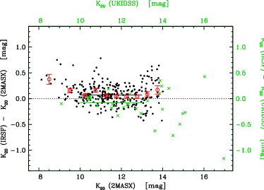
Figure 1: Difference between $K_{20}$ magnitudes from IRSF and 2MASX (black dots) and IRSF and UKIDSS (green crosses) as a function of 2MASX $K_{20}$. The average difference over the $10^{\rm m}-13^{\rm m}$ range in $K_{20}$ is indicated by a horizontal black and green line, for IRSF – 2MASX and IRSF – UKIDSS, respectively. The red open circles indicate binned means and errors of IRSF – 2MASX magnitudes between $8^{\rm m}$ and $14^{\rm m}$ in $K_{20}$. For comparison, the dotted line indicates a zero difference.

The effects of the cases where the automated photometry failed (Item 4.) can go either way: where the position angle is wrong or the size too small the $K_{\rm s}$-band magnitude will be (slightly) underestimated, while in cases where the size was overestimated (due to non-subtracted star(s) near the galaxy) the $K_{\rm s}$ magnitude will be overestimated. In addition, other non-subtracted stars within the aperture (but not affecting the position angle), will also lead to $K_{\rm s}$-band magnitudes that are too bright.

An overall comparison of the 2MASX photometry with that from deeper NIR images obtained at the InfraRed Survey Facility (IRSF) telescope at the South African Astronomical Observatory was made by Said et al. (2016): see their Figure 7 for a comparison of the 2MASX isophotal $K_{20}$ and IRSF magnitudes, and also their Figure 8 for a comparison between IRSF and UKIDSS magnitudes. They report good agreement for the range $9^{\rm m}-14^{\rm m}$. Using the same datasets, we find (see Fig. 1) the 2MASX $K_{20}$ magnitudes to be on average $0\aas@@fstack{m}071\pm 0\aas@@fstack{m}012$ brighter than those of the deeper IRSF images (black dots) in the $K_{20}$ range $10^{\rm m}-13^{\rm m}$ ($N=207$). This value compares well with the value of $0\aas@@fstack{m}08\pm 0\aas@@fstack{m}01$ value obtained by Williams et al. (2014) for 102 galaxies in the precursor project. Furthermore, we find that IRSF $K_{20}$ magnitudes are brighter by $0\aas@@fstack{m}078\pm 0\aas@@fstack{m}035$ compared to the UKIDSS measurements (green crosses). This results in a total offset of $0\aas@@fstack{m}15\pm 0\aas@@fstack{m}04$ between 2MASX and UKIDSS photometry.

As argued by Williams et al. (2014), the obvious explanation is that unresolved faint stars are the cause of this offset. Nevertheless, we do not find any dependence of the offset with stellar densities (nor with colour or extinction) for this data set. We thus conclude that the effect of unresolved stars on the photometry is already present at the moderate stellar density level of $\log N_{*}/{\rm deg}^{2}$ = 3.5 (i.e., the lower limit for this data set). Further investigation is required to determine at which stellar density this effect becomes important.

In addition, Andreon (2002) and Kirby et al. (2008) report that 2MASX isophotal fluxes in general are underestimated by more than 20%, which is assumed to be due to the short exposure times used by 2MASS (this also affects any luminosity functions derived from 2MASX isophotal fluxes, as discussed in detail by Andreon 2002). This would mean that 2MASX galaxies in the ZoA are too bright by at least $0\aas@@fstack{m}35$ magnitudes as compared to higher latitude 2MASX galaxies (assuming the UKIDSS GPS photometry, used as reference, is accurate, and because the UKIDSS photometry are calibrated using 2MASS stars) since a 2MASX galaxy is $0\aas@@fstack{m}20$ too faint compared to deeper photometry but, in the ZoA, they are found to be $0\aas@@fstack{m}15$ too bright instead. This needs to be taken into account when combining our sample with the 2MRS and 2MTF samples.

Finally, we can estimate the uncertainty in the limiting magnitude of our sample to be $0\aas@@fstack{m}15$ based on the scatter of the IRSF – 2MASX magnitude difference in the 2MASX magnitude bin $11^{\rm m}-11\aas@@fstack{m}5$.

3.2 Correction for Galactic extinction

We used the DIRBE/IRAS FIR maps (SFD98) to extract extinction information; these maps, however, are uncalibrated at low Galactic latitudes ($|b|<5\degr$). Among others, Schröder et al. (2007) used NIR galaxy photometry of a cluster around PKS 1343–601 to derive a correction factor of 0.87 to $E(B-V)$ at low latitudes, and SF11 determined that the whole-sky SFD98 maps had to be recalibrated by applying a factor of 0.86. We prefer SFD98 over other maps in the literature (e.g., Planck Collaboration et al. 2016) since they are used widely, and our values are thus consistent with 2MRS and 2MTF surveys. In a forthcoming paper (Schröder et al., Paper III) we will present a detailed comparison.

We decided not to use the SF11 correction factor of 0.86 in our sample selection so as to remain consistent with the 2MRS sample definition. This correction factor can always be applied at a later stage and the sample will still be complete. Note that only 204 galaxies ($<6$%) would become fainter than the magnitude cut-off if this correction factor were applied.

Around some objects the foreground extinction shows a strong, local spatial variation which is not reflected in the DIRBE/IRAS maps given their relatively coarse pixel size of $6\arcmin$$\times$$6\arcmin$. Wherever the $10\arcmin$$\times$$10\arcmin$ $B$- or $R$-band images showed such obvious small-scale variations, we set an extinction flag. Sometimes a variation across the image was discernible but without the sharp edges typical of a dark cloud; in these cases we set a flag indicating that the extinction could be wrong. Note that this was done systematically for galaxies only. A total of 217 galaxies are affected; these flags are entirely based on visual impression and are not complete. Notable is also that the extinction is more likely to fluctuate on small scales where it is intrinsically high (that is, in the area of dark clouds or Galactic nebulae).

In regions where extinction shows strong spatial variations, the true extinction may be either higher or lower, and the effect of extinction on the sample selection cannot be estimated. Based on the above-mentioned numbers, though, the effect is deemed to be small.

3.3 Additional Galactic extinction corrections

For determining isophotal magnitudes the applied Galactic foreground extinction correction is not sufficient (Cameron 1990, Riad et al. 2010): the dust in the Milky Way forms a screen which lowers the surface brightness of any galaxy behind it, and therefore reduces their observed radius (e.g., at the 20^th mag arcsec^-2 level). We therefore need to correct the observed $K_{20}$ isophotal diameter for this effect and hence also the isophotal magnitude.

We have followed the method outlined by Riad et al. (2010) using the 2MASX central surface brightness (k_peak), since 2MASX does not supply a disc central surface brightness as required for an optimal correction. The method also requires knowledge of the morphological type, since the surface brightness profiles of elliptical and spiral galaxies (or bulges and discs) follow different laws. However, morphological classification is more difficult in the NIR compared to the optical, and even more so in the ZoA where the disc is partly or even fully obscured. We therefore decided to apply the correction for spiral galaxies to all objects in our catalogue, keeping in mind that (a) only about 20% of all galaxies are ellipticals, (b) one could use the disc class parameter (Sec. 2.3) to distinguish between spirals and ellipticals (see discussion below), and (c) we are mainly interested in the Tully–Fisher relation which only applies to spiral galaxies. To optimise this correction, though, we also applied the correction factor 0.86 to the $E(B-V)$ values (SF11).

The effect of the additional extinction correction is complex: the SF11 correction to the $E(B-V)$ values makes galaxy magnitudes fainter, but the diameter correction is additive and thus makes magnitudes brighter. Therefore, some previously too faint objects would now lie above our $11\aas@@fstack{m}25$ magnitude limit, and some sample objects would become fainter. To investigate this effect we flagged all objects from our sample that would be excluded when using the fully corrected magnitudes $K^{\rm o,d}_{\rm s}$ (Col. 7d), and we extracted all objects from the 2MASX catalogue that would be added to the sample (presented in the appendix). We thus would have an additional 70 and 1 galaxies in the ZOA and EBV samples, respectively, but would also lose 29 and 0, respectively, which means that the sample size would increase marginally by about 1% due to an improved extinction correction.

We corrected the major-axis diameters $a$ and the $K_{\rm s}$-band magnitudes for the diameter-dependent extinction, but not the colours: this because the 2MASX $J$- and $H$-band ‘isophotal’ magnitudes, from which the colours are derived, refer to the $K_{\rm s}$-band isophotal fiducial elliptical aperture and not a fixed isophote in the $J$- and $H$-bands. Since the NIR colours of galaxies change only slowly with radius (especially in the outer parts; Jarrett et al. 2003), the conventional extinction corrected colours out to the uncorrected isophotal radius will be sufficient for our purposes and, in particular, they do not affect the sample definition. To be consistent with the $K^{\rm o,d}_{\rm s}$ magnitudes though, we did apply the correction factor 0.86 (SF11) to the colours (denoted $(H-K_{\rm s})^{\rm o,c}$ and $(J-K_{\rm s})^{\rm o,c}$ ).

For elliptical galaxies the corrections are smaller than for spirals due to their steeper surface brightness profiles. Since we applied the correction for spirals to all objects, the $K^{\rm o,d}_{\rm s}$-sample size would decrease slightly if we could properly distinguish elliptical from spiral galaxies. We preferred not to make such a distinction using the disc parameter (see Sec. 5.4 for more details) for the following reasons: (a) The radial profiles of spiral galaxies (and thus the correction) also vary with morphological subtype, hence the uncertainty in the correction at higher extinctions quickly becomes significant. (b) The uncertainty in the correction method we used is larger than for the optimal correction method which uses the disc central surface brightness (see the detailed discussion in Riad et al. 2010). (c) The disc parameter is only reliable in those cases where a disc is noticeable; it is more uncertain when discriminating elliptical from early-type spiral galaxies (classes ‘D3’ and ‘D4’), in particular at higher extinctions where only bulges of spiral galaxies might be visible (and thus a correction is technically not applicable anyway). (d) It is not clear what kind of correction to use for the disc classes ‘D3’ and ‘n’ which make up about 18% of the galaxy sample. In other words, using the disc parameter for the extinction correction would only introduce an unknown uncertainty which may or may not be larger than the correction applied.

The caveats outlined here indicate that we need to be cautious when applying this additional correction. We therefore restricted ourselves to the conventional extinction correction. The additional galaxies presented in the appendix will be used for further discussions on selection effects in later analyses; they will be important also for the TF analysis.

3.4 Preparing for the Tully-Fisher application

In preparation for the cosmic flow fields analysis (see Sec. 1) we determined which galaxies are potentially useful for inclusion in the Tully-Fisher (TF) sample. Since the inclination corrections to the line widths dominate the errors in the TF relation (note they are also used in the internal absorption corrections in the TF relation, which however are small in the NIR, see Table 1), we selected only ‘sufficiently’ inclined galaxies for this sample, that is, galaxies with minor/major axial ratios (2MASX parameter sup_ba) of $b/a\leq 0.5$; at relatively high extinction values, i.e., $A_{\rm K}\geq 0\aas@@fstack{m}50$, we also selected galaxies with a generous $0.5<b/a\leq 0.7$ to account for the fact that obscured galaxies appear rounder (Said et al., 2015). We thus have selected 1296 galaxies from our ZoA sample and a further 35 galaxies from the EBV sample (that is, 35% and 40% of the total samples, respectively).

Unlike the 2MTF survey we have not applied any further selection on galaxy type. Although we could use the disc class parameter, a low surface brightness disc can easily be missed in the ZoA. Instead, we flagged all galaxies in this potential TF sample for H I observations. Our final TF sample to be used for cosmic flow studies will be based on their H I detection (see Paper II).

The photometry problems regarding the definition of the fiducial elliptical aperture mentioned in Sec. 3.1 also affect the TF sample definition: while most problems concern only the major axis position angle (which can also affect the magnitude of a galaxy), in some cases the axial ratio is affected and thus the derived inclination is incorrect. The effect on inclination is small: based on visual inspection only an estimated $2-3$% of the total sample seems to have obviously incorrect inclinations (see Item 4. in Sec. 3.1). Note that for the final TF sample selection and application all galaxies will be re-reduced and individually inspected to ensure a high quality and consistency in all parameters (see, for example, Said et al. 2016). The extinction correction to the axial ratios (Said et al., 2015) will be applied at this stage leading to a final cut in $b/a$, thus rendering the final TF sample complete and independent of the above mentioned photometry problems.

4 The catalogue

The catalogue of the 6913 ZOA objects and the 502 EBV objects is available online only as Tables 3a and 3b, respectively; an example page is given below in Table LABEL:zoatabex.

The columns are as follows:

Col. 1: ID: 2MASX catalogue identification number (based on J2000.0 coordinates);

Col. 2a and 2b: Galactic coordinates: longitude $l$ and latitude $b$, in degrees;

Col. 3: Extinction: $E(B-V)$ value derived from the DIRBE/IRAS maps (SFD98), in mag;

Col. 4: Object flag: 1 = obvious galaxy, 2 = galaxy, 3 = probable galaxy, 4 = possible galaxy, 5 = unknown, 6 = lower likelihood for galaxy, 7 = unlikely galaxy, 8 = no galaxy, 9 = obviously not a galaxy;

Col. 5: Object offset flag: ‘o’ stands for coordinates that are offset from the centre of the object, and ‘e’ stands for detections near the edge of an image (at an offset position from the object centre) which were detected with properly centred coordinates on the adjacent image;

Col. 6: Object class: ‘p’ stands for PN, ‘p?’ for possible PN, ‘s’ for a probable DIRBE/IRAS point source that was not removed from the extinction maps (only the case if $|b|<5\degr$) and the extinction is likely to be overestimated, and ‘s?’ stands for a possible DIRBE/IRAS point source (see Sec. 5.3);

Col. 7a: Sample flag galaxy: ‘g’ denotes a galaxy (object classes $1-4$), and ‘p’ stands for galaxy candidates (class 5);

Col. 7b: Sample flag TF: ‘t’ means the galaxy is inclined enough to be nominally included in the sample for application of the Tully-Fisher relation (see Sec. 3.4);

Col. 7c: Sample flag H I observation: ‘N’ means the object was observed by us in the 21cm H I line with the NRT (see Paper III), ‘P’ means the object was observed by us with the Parkes radio telescope (publication in preparation), and a ‘+’ indicates that the object still needs to be observed for a redshift;

Col. 7d: Sample flag extended sample: Objects that will not be included in the extended sample based on the diameter-extinction correction ($K^{\rm o,d}_{\rm s}$ $\leq 11\aas@@fstack{m}25$) are marked with a star;

Col. 8: Galaxy disc type: ‘D1’ means an obviously visible disc and/or spiral arms, ‘D2’ stands for a noticeable disc, ‘D3’ for a possible disc, and ‘D4’ stands for no disc noticeable. Where it was not possible to tell (likely due to adjacent or superimposed stars or very high extinction) we give a flag ‘n’;

Col. 9: 2MRS flags: ‘c’ stands for an entry in the main catalogue, and ‘e’ for the extra catalogue (that is, outside the 2MRS selection criteria) . For the sub-catalogues we give: ‘cf’ for an entry in the flg catalogue (affected by nearby stars, but not severely), ‘cp’ for an entry in the flr catalogue (severely affected by nearby stars), ‘ca’ and ‘ea’ are objects that have been reprocessed and are both in the rep as well as add catalogues (in the latter case with new IDs and photometry, not listed by us), ‘cr’ and ‘er’ are objects rejected as galaxies and which can be found in the rej catalogues, ‘cn’ and ‘en’ are objects that have no redshifts yet and are listed in the nocz catalogues;

Cols. 10a and 10b: Velocity measurement flags ‘vo’ and ‘vh’ from the literature: ‘o’ stands for an optical measurement and ‘o?’ indicates a questionable optical measurement or object ID, ‘g’ the velocity shows it to be a Galactic object, ‘h’ stands for published H I velocity and ‘h:’ for uncertain H I velocity, ‘h?’ is an uncertain object ID (based on a radio telescope’s large beam size that may include nearby galaxies), and a star ‘*’ in either column stands for a yet unpublished measurement (see Sec. 2.2);

Col. 11: Deep NIR image flag: ‘U’ indicates there is a UKIDSS image for this object, and ‘V’ stands for VISTA;

Col. 12: Photometry flag (Sec. 3.1): the 2MRS flags for questionable photometry (see Col. 9) are repeated here: ‘a’ stands for improved photometry exists, ‘p’ for photometry is severely compromised, and ‘f’ for poor photometry; in addition, ‘c’ denotes improved photometry exists in John Huchra’s original list, and ‘o’ stands for offset (see Col. 4);

Col. 13: Extinction flag (see Sec. 3.2): ‘e’ stands for a likely wrong extinction value, either due to small-scale variations or a non-removed IRAS/DIRBE point source, ‘e?’ denotes a possible wrong extinction value;

Col. 14: 2MASX magnitude $K_{\mathrm{2}0}$: isophotal $K_{\rm s}$-band magnitude measured within the $K_{\rm s}$-band 20 mag arcsec^-2 isophotal elliptical aperture (in mag);

Cols. 15 and 16: 2MASX colours $(H-K_{\rm s})$ and $(J-K_{\rm s})$: isophotal colours measured within the $K_{\rm s}$-band 20 mag arcsec^-2 isophotal elliptical aperture (in mag);

Col. 17: 2MASX flag $vc$: the visual verification score of a source (see Sec 5.1);

Col.18: 2MASX object size $a$: the major diameter of the object, which is twice the 2MASX $K_{\rm s}$-band 20 mag arcsec^-2 isophotal elliptical aperture semi-major axis r_k20fe (in arcseconds);

Col. 19: 2MASX axis ratio $b/a$: minor-to-major axis ratio fit to the $3\sigma$ super-co-added isophote, sup_ba. Single-precision entries are given in cases where the 2MASX parameter sup_ba is not determined; these values were estimated from the axial ratios available in the different passbands;

Col. 20: 2MASX stellar density: co-added logarithm of the number of stars ($K_{\rm s}$$<14$ mag) per square degree around the object;

Cols. 21 – 23: Magnitude $K^{\rm o}_{\rm s}$ and colours $(H-K_{\rm s})^{\rm o}$ and $(J-K_{\rm s})^{\rm o}$ corrected for foreground extinction (Col. 3) as described in Sec. 2.1 (in mag);

Col. 24: Extinction in the $K_{\rm s}$-band $A_{\rm K}$: calculated from $E(B-V)$ in Col. 4 and applying the SF11 correction of 0.86 (in mag);

Col. 25: Extinction corrected major diameter $a^{\rm d}$ according to Riad et al. (2010) using $E(B-V)$ from Col. 4 with the SF11 correction factor 0.86; only given for objects classified as galaxies (in arcseconds), see Sec. 3.3;

Col. 26: Extinction corrected magnitude $K^{\rm o,d}_{\rm s}$ corrected according to Riad et al. (2010) using $E(B-V)$ from Col. 4 with the SF11 correction factor 0.86; only given for objects classified as galaxies (in mag) (see Sec. 3.3);

Cols. 27 and 28: Extinction corrected colours $(H-K_{\rm s})^{\rm o,c}$ and $(J-K_{\rm s})^{\rm o,c}$ using $E(B-V)$ from Col. 4 with the SF11 correction factor 0.86 (in mag).

Table 3: 2MASS ZoA sample; example page, the full table is available online

2MASX J	$l$	$b$	EBV	Object			Sample				Disc	2MRS	Velocity		NIR	Photom	Ext	$K_{20}$	$H$-$K$	$J$-$K$	vc	$a$	$b/a$	st.d.	$K^{\rm o}_{\rm s}$	($H$-$K)^{o}$	($J$-$K)^{o}$	$A_{\rm K}$	$a^{\rm d}$	$K^{\rm o,d}_{\rm s}$	($H$-$K)^{o,c}$	($J$-$K)^{o,c}$
	deg	deg	mag	class	off	flg	gal	TF	obs	ext’d	type		Opt	HI	flg	flg	flg	mag	mag	mag		”			mag	mag	mag	mag	′′	mag	mag	mag
(1)	(2a)	(2b)	(3)	(4)	(5)	(6)	(7a)	(7b)	(7c)	(7d)	(8)	(9)	(10a)	(10b)	(11)	(12)	(13)	(14)	(15)	(16)	(17)	(18)	(19)	(20)	(21)	(22)	(23)	(24)	(25)	(26)	(27)	(28)
00000637$+$5319136	115.217	$-8.780$	$0.300$	1	$-$	$-$	g	$-$	$-$	$-$	D4	c	o	$-$	$-$	$-$	$-$	$11.196$	$0.42$	$1.15$	$1$	35.0	$0.90$	$3.59$	$11.084$	$0.37$	$1.00$	0.09	$35.6$	$11.09$	$0.38$	$1.02$
00000702$+$6717254	117.996	$4.912$	$10.331$	9	$-$	$-$	$-$	$-$	$-$	$-$	$-$	$-$	$-$	$-$	$-$	$-$	$-$	$13.614$	$0.53$	$1.38$	$-1$	11.0	$1.00$	$3.63$	$9.765$	$-1.18$	$-3.75$	3.20	$\cdots$	$\cdots$	$-0.98$	$-3.07$
00001859$+$6716444	118.012	$4.897$	$9.743$	9	$-$	$-$	$-$	$-$	$-$	$-$	$-$	$-$	$-$	$-$	$-$	$-$	$-$	$14.306$	$0.36$	$1.30$	$-1$	10.0	$1.00$	$3.63$	$10.676$	$-1.26$	$-3.54$	3.02	$\cdots$	$\cdots$	$-1.06$	$-2.89$
00002049$+$6717044	118.016	$4.902$	$9.880$	9	$-$	$-$	$-$	$-$	$-$	$-$	$-$	$-$	$-$	$-$	$-$	$-$	$-$	$13.371$	$0.60$	$1.61$	$-1$	19.4	$0.54$	$3.63$	$9.690$	$-1.04$	$-3.30$	3.06	$\cdots$	$\cdots$	$-0.84$	$-2.65$
00003760$+$6735164	118.103	$5.194$	$4.645$	8	$-$	$-$	$-$	$-$	$-$	$-$	$-$	$-$	$-$	$-$	$-$	$-$	$-$	$12.242$	$0.50$	$1.47$	$-2$	22.6	$0.34$	$3.91$	$10.511$	$-0.27$	$-0.83$	1.44	$\cdots$	$\cdots$	$-0.18$	$-0.53$
00003769$+$6710184	118.021	$4.786$	$6.767$	8	$-$	$-$	$-$	$-$	$-$	$-$	$-$	$-$	$-$	$-$	$-$	$-$	$-$	$12.635$	$1.11$	$\cdots$	$1$	37.2	$0.46$	$3.63$	$10.114$	$-0.01$	$\cdots$	2.10	$\cdots$	$\cdots$	$0.12$	$\cdots$
00004194$+$6838344	118.318	$6.227$	$0.957$	7	$-$	$-$	$-$	$-$	$-$	$-$	$-$	$-$	$-$	$-$	$-$	$-$	$-$	$9.622$	$1.60$	$3.34$	$1$	23.2	$0.78$	$3.67$	$9.265$	$1.44$	$2.87$	0.30	$\cdots$	$\cdots$	$1.46$	$2.93$
00004647$+$6732523	118.109	$5.152$	$6.505$	8	$-$	$-$	$-$	$-$	$-$	$-$	$-$	$-$	$-$	$-$	$-$	$-$	$-$	$10.986$	$1.17$	$3.21$	$1$	42.4	$0.62$	$3.91$	$8.562$	$0.09$	$-0.02$	2.01	$\cdots$	$\cdots$	$0.22$	$0.41$
00013723$+$6436560	117.623	$2.259$	$4.572$	9	$-$	$-$	$-$	$-$	$-$	$-$	$-$	$-$	$-$	$-$	$-$	$-$	$-$	$12.737$	$0.35$	$1.33$	$-2$	17.8	$0.70$	$3.94$	$11.033$	$-0.41$	$-0.95$	1.42	$\cdots$	$\cdots$	$-0.32$	$-0.64$
00013755$+$6437360	117.626	$2.270$	$4.633$	9	$-$	$-$	$-$	$-$	$-$	$-$	$-$	$-$	$-$	$-$	$-$	$-$	$-$	$11.735$	$0.41$	$1.23$	$1$	37.2	$0.80$	$3.94$	$10.009$	$-0.36$	$-1.08$	1.44	$\cdots$	$\cdots$	$-0.27$	$-0.77$
00014201$+$6724323	118.169	$4.999$	$7.957$	8	$-$	$-$	$-$	$-$	$-$	$-$	$-$	$-$	$-$	$-$	$-$	$-$	$-$	$13.778$	$0.56$	$1.28$	$-1$	13.6	$1.00$	$3.94$	$10.813$	$-0.76$	$-2.67$	2.46	$\cdots$	$\cdots$	$-0.60$	$-2.14$
00014668$+$6708413	118.126	$4.738$	$4.218$	8	$-$	$-$	$-$	$-$	$-$	$-$	$-$	$-$	$-$	$-$	$-$	$-$	$-$	$11.590$	$1.18$	$2.17$	$1$	61.8	$0.52$	$3.79$	$10.018$	$0.48$	$0.07$	1.31	$\cdots$	$\cdots$	$0.57$	$0.35$
00031331$+$5352149	115.783	$-8.330$	$0.299$	1	$-$	$-$	g	$-$	$-$	$-$	D3	c	o	$-$	$-$	$-$	$-$	$10.252$	$0.37$	$1.20$	$1$	48.6	$0.78$	$3.57$	$10.141$	$0.32$	$1.05$	0.09	$49.3$	$10.15$	$0.33$	$1.07$
00033726$+$6919064	118.707	$6.840$	$0.808$	2	$-$	$-$	g	$-$	$-$	$-$	D4	c	o	$-$	$-$	$-$	$-$	$11.480$	$0.40$	$1.50$	$1$	26.4	$0.70$	$3.60$	$11.179$	$0.27$	$1.10$	0.25	$28.1$	$11.19$	$0.28$	$1.15$
00034142$+$7036434	118.955	$8.110$	$0.789$	1	$-$	$-$	g	$-$	$-$	$-$	D1	c	o	$-$	$-$	$-$	$-$	$11.544$	$0.35$	$1.29$	$1$	36.6	$0.68$	$3.55$	$11.250$	$0.22$	$0.90$	0.24	$39.4$	$11.24$	$0.23$	$0.95$

Table 3: continued.

5 Properties of the catalogue

5.1 Distinguishing galaxies from non-galaxies

The cleanliness of the galaxy catalogue (i.e., its contamination by non-galaxies) can be visualised in a colour-colour plot such as Fig. 2. The colours are corrected for Galactic foreground extinction according to SFD98 (see Sec. 2); please note that a change in calibration in extinction as discussed in SF11 and Paper III introduces a stretching in colours but does not affect the qualitative discussion presented here. Figure 2 shows objects classified as galaxies in black and non-galaxies in yellow; the few galaxy candidates (objects of unknown classification, class 5) are shown in green. Objects we identified as Planetary Nebulae (PNe; based on information in the literature or through visual inspection) are marked in blue (where open blue circles denote possible PNe). They are clearly offset in $(H-K_{\rm s})^{\rm o}$ colour. Also shown is the reddening path for the intrinsic colour range occupied by the bulk of the galaxies (in-between the two dashed lines). Galaxies with questionable extinctions (based on visually obvious variations across the images), which are marked with large red circles, are scattered along the reddening path. The plot suggests that all galaxies with unusual $(H-K_{\rm s})^{\rm o}$/ $(J-K_{\rm s})^{\rm o}$ colour combinations in the reddening path have incorrect extinction values attributed to them. However, galaxies outside the reddening path are likely to be affected by starlight in the photometry aperture. In other words, although we used the colour-colour plot during the visual screening process to help distinguish some of the galaxy candidates from other types of objects, this was not always possible, in particular for objects within or near the reddening path (see, for example, objects classified as ‘unknown’).

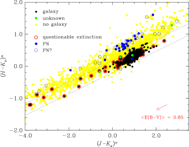
Figure 2: 2MASS extinction-corrected colour-colour plot: $(H-K_{\rm s})^{\rm o}$ as a function of $(J-K_{\rm s})^{\rm o}$ for all 2MASX objects in the ZOA and EBV samples. The reddening path for objects within the intrinsic colour range of galaxies is indicated with two parallel dashed lines. A reddening vector, representing the mean $E(B-V)$ $=0\aas@@fstack{m}85$ of the sample, is shown as a red arrow in the bottom right corner. Black dots indicate galaxies, yellow dots non-galaxies, green dots objects of unknown nature, blue dots PNe and blue circles possible PNe; red circles denote objects with questionable Galactic extinction.

We have made a similar colour-colour plot for the WISE bands $W1$ ($\lambda=3.4\mu$m), $W2$ ($\lambda=4.6\mu$m) and $W3$ ($\lambda=12\mu$m) using aperture 1 ($5\aas@@fstack{\prime\prime}5$) data of the ALLWISE catalogue Figure 3 shows the extinction-corrected colour $(W1-W2)^{o}$ as a function of $(W2-W3)^{o}$ using the same symbols as in Fig. 2. Using these colours, spiral galaxies and ellipticals are separated in ($W2-W3$) (to the right and the left, respectively, see Figure 26 in Jarrett et al. 2011), while active and intensely star forming galaxies are separated in ($W1-W2$) (top). Unlike for 2MASS colours, though, the PNe are not clearly offset from the galaxies: their colours overlap with those of starburst or otherwise active galaxies.

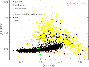
Figure 3: WISE colour-colour plot: $(W1-W2)^{o}$ as a function of $(W2-W3)^{o}$ for all 2MASX objects in our ZOA and EBV samples. The symbols are as in Fig. 2.

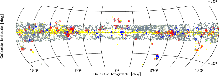
Figure 4: Aitoff projection in Galactic coordinates of the ZOA and EBV samples. The symbols used are basically the same as in Fig. 2 except that grey is used here for galaxies for better distinction.

The on-sky distribution of both the ZOA and the EBV samples is shown in Fig. 4 with the basically same colour scheme as for Figs 2 and 3, except that galaxies are shown in grey here for clarity. There are only a few areas at higher latitudes ($b\geq 10$°) that have extinctions high enough to be in the EBV sample. Most of the non-galaxies are close to the Galactic Plane which is expected since the contamination of the 2MASX catalogue with blended stars or with stars close to diffraction spikes of bright stars is small, and most of the non-galaxian detections are caused by Galactic Nebulae.

The 2MASX catalogue gives a parameter vc which is a visual verification score (Jarrett et al., 2000). It distinguishes between extended sources (vc $=1$) and blended stars or artefacts (vc $=2$). In quite a few cases the flags for ‘unknown’ (vc $=-2$; $N=573$) and ‘not examined’ (vc $=-1$; $N=209$) are given. There is only one case where we identified a vc-flag 2 object as a galaxy: 2MASX J18531497$-$0623155 is a tiny galaxy next to an equally bright star and could only be unambiguously identified as a galaxy on a UKIDSS image. This is a good example of a case where the superimposed star was not subtracted from the photometry and the galaxy itself is actually too faint for our nominal magnitude limit.

5.2 Completeness

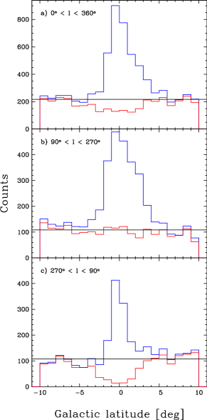
Figure 5: Histograms of objects in the ZOA sample as a function of Galactic latitude for all objects (blue) and for galaxies only (red). The black line represents the average 2MASX bright galaxy count outside the ZoA. Panel (a): for all Galactic longitudes; panel (b) for the semi-circle towards the anti-centre region; panel (c) for the semi-circle towards the bulge.

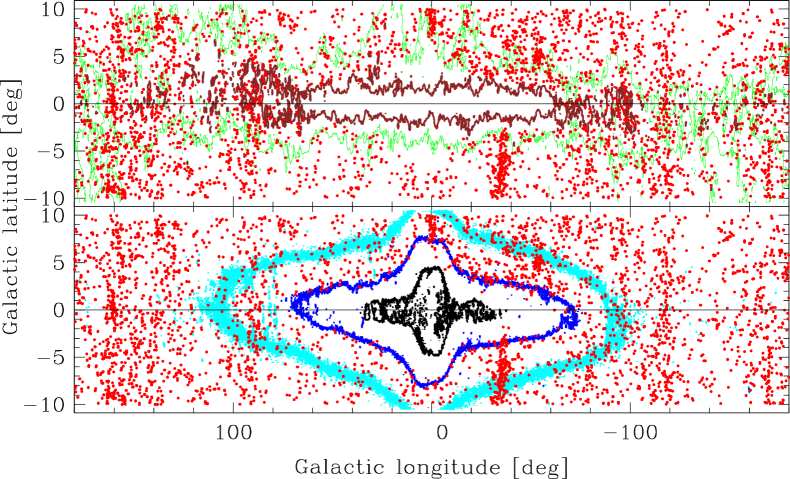
Figure 6: Sky maps with contours of Galactic extinction (top) and stellar density (bottom) in the ZoA. Galaxies are indicated by red dots. Top panel: extinction contour levels shown are $A_{\rm K}=0\aas@@fstack{m}3$ (green) and $1\aas@@fstack{m}0$ (brown); bottom panel: stellar density contour levels shown are $\log N_{*}/{\rm deg}^{2}=4.0$ (light blue), 4.5 (dark blue) and 5.0 (black).

Most galaxy samples become incomplete at lower latitudes, and a lack of galaxies in our sample in the Galactic bulge area is obvious from Fig. 4. To test the completeness of the ZOA sample, we show in Fig. 5 (top panel) the histogram of source counts as a function of Galactic latitude for all 6913 objects in our ZOA sample (blue) and of the 3675 ZOA galaxies only (red). The black line represents the average number of galaxies outside the ZoA of 0.605 galaxies/sq.deg, as derived from the 2MASX catalogue for $|b|>10\degr$ and $K_{\rm 20}\leq 11\aas@@fstack{m}25$, multiplied by the area covered in each bin. The histogram for the galaxies shows a dip for $\sim-6\degr<b<3\degr$, which means, in this range we are incomplete. The dip disappears towards the anti-centre region ($90\degr<l<270\degr$, middle panel), while it is deeper for the bulge region ($90\degr>l$ and $l>270\degr$, lower panel).

If we select only those latitudes bins with galaxy counts comparable to the average number outside the ZoA (i.e., $-10\degr<b<-6\degr$ and $3\degr<b<10\degr$), we find 2341 galaxies in our sample, while based on the average 2MASX galaxy count outside the ZoA we would expect 2381 galaxies. The difference of 41 galaxies is smaller than the $1\sigma$ Poissonian error of 49 and therefore negligible. We thus conclude that, in combination with the all-sky 2MASX sample, we are now complete below $b=-6\degr$ and above $b=3\degr$, and the 2MASX bright galaxy ZoA is reduced to a strip of 9°width in Galactic latitude. In the anti-centre region the ZoA has all but disappeared.

We also note a slight slope with latitude in the lower two panels: while towards the anti-centre region the area above the Galactic plane shows fewer galaxies than below the plane (345 and 489 for the four outermost bins, respectively), the trend is reversed for the Galactic bulge region: 466 and 395, respectively. This asymmetry seems to be entirely due to large scale structures and varies depending on where the longitude cuts are set.

Both effects are also evident in the on-sky distribution of the ZOA galaxies as shown in Fig. 6 (red dots): the top panel displays contours of Galactic extinction, and the bottom panel shows contours of stellar density as derived from the 2MASS Point Source Catalogue. While the distribution of galaxies is influenced by density variations due to obvious large scale structures, it is evident that the lack of 2MASX galaxy detections towards the Galactic bulge region is mainly due to the high stellar density: we lose completeness at around or slightly above the $\log N_{*}/{\rm deg}^{2}$ = 4.5 level (dark blue contour); the extinction contours cannot explain in particular the lack of 2MASX galaxies at the higher latitudes around the Galactic Centre. On the other hand, even at extinctions as high as $A_{\rm K}=1\aas@@fstack{m}0$ (brown contour) it is possible to detect 2MASX galaxies. Note also the slight tilt angle in the contours of both extinction and stellar densities which is due to the Galactic warp (e.g., Reylé et al. 2009).

For a more quantitative analysis, we can use histograms of galaxy counts as a function of extinction and stellar density. A comparison is only useful, however, if we take into account the variation in sky area per bin. We have thus binned the extinction and stellar density data in the ZoA (excluding the EBV sample) and derived number density values (per sq.deg) as shown in Fig. 7 (red for galaxies, blue for all objects).

The number density of galaxies remains remarkably constant across all stellar densities in the ZoA except for the lowest and highest values (top panel): for $\log N_{*}/{\rm deg}^{2}<3.4$ the overall area is very small (3%), whereas the abrupt cut-off at $\log N_{*}/{\rm deg}^{2}>4.5$ is due to incompleteness (see also Jarrett et al. 2000). The bin-to-bin variations in the range $3.4-4.5$ are most likely due to variations in large-scale structures. The histogram also shows that the non-galaxy population (the difference between the blue and red histograms) increases rapidly with stellar density up to $\log N_{*}/{\rm deg}^{2}\sim 4.0$ and accounts for most 2MASX detections at $\log N_{*}/{\rm deg}^{2}>4.5$ (87%).

To investigate whether extinction has any effect on the completeness we first excluded all areas with stellar densities $\log N_{*}/{\rm deg}^{2}>4.5$ (to avoid a selection bias since both high extinction and high stellar density occur in similar areas, see Fig. 6). The resulting histogram is shown in the bottom panel of Fig. 7. The number densities are highly affected by low number statistics for $A_{\rm K}\,\lower 1.99997pt\hbox{$\buildrel>\over{\sim}$}\,1\aas@@fstack{m}0$ (88 galaxies). All the bins up to $A_{\rm K}=2\aas@@fstack{m}0$ are consistent within the errors with the high-latitude 2MASX galaxy density of 0.605 galaxies/sq.deg (dotted line). The slight apparent drop off from $A_{\rm K}\sim 0\aas@@fstack{m}6$ towards $1\aas@@fstack{m}4$ is not significant and could also be due to variations in large scale structures.

Our conclusion is that the 2MASX sample of $K^{\rm o}_{\rm s}$ $\leq 11\aas@@fstack{m}25$ is complete over the whole sky wherever $\log N_{*}/{\rm deg}^{2}<4.5$ and at least where $A_{\rm K}<0\aas@@fstack{m}6$ (or $E(B-V)=1\aas@@fstack{m}61$), and likely up to $A_{\rm K}\sim 2\aas@@fstack{m}0$ (or $E(B-V)=5\aas@@fstack{m}37$). Thus the NIR ‘bright galaxies’ ZoA has been reduced to cover only 2.4% of the whole sky as compared to the over 20% for the original optical ZoA (based on a diameter limit of $1\arcmin$, see Kraan-Korteweg & Lahav 2000) and 9.6% for 2MRS.

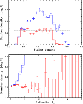
Figure 7: Histograms of the number density of all ZOA sample objects (blue) and galaxies only (red) as a function of stellar density (top panel) and Galactic extinction $A_{\rm K}$ (bottom panel; only regions with $\log N_{*}/{\rm deg}^{2}\leq 4.5$ were used). The error bars indicate Poissonian errors per bin. The black dotted lines represent the average 2MASX bright galaxy number density outside of the ZoA.

5.3 Extinction

We have set two flags in the catalogues regarding potential extinction problems: (i) for objects lying in areas where we suspect that the extinction varies rapidly we have set an extinction flag (Col. 13; see also Figs 2 – 4); (ii) for objects that seem to be either a source in the DIRBE/IRAS FIR maps or affected by one, we have set an object class (Col. 6) which was determined as follows.

In the SFD98 maps, FIR sources (mostly extragalactic, but also unresolved Galactic sources) were removed for $|b|>5\degr$. At lower latitudes, sources were only removed from some selected (unconfused) areas. The output of the query script for a given position gives flags whether a source list exists, and if a source has been subtracted. For 3184 objects and 2476 galaxies a source list was available, with a source being subtracted in 702 and 541 cases, respectively.

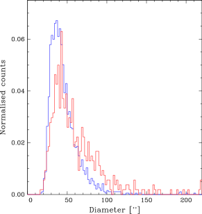
Figure 8: Normalised histogram of major axis diameters of galaxies (in arcseconds) for those galaxies where a DIRBE/IRAS FIR source list was used in the making of the SFD98 Galactic extinction maps. Red: all positions where a source was subtracted, blue: all other positions.

Next, we investigated the SFD98 maps of all our galaxies for which no DIRBE/IRAS source list exists ($N=1287$) to establish whether the position might be affected by an unsubtracted point source. We compared the extinction value at the target position to those measured at four positions offset by seven arcminutes. Furthermore we investigated all galaxies with a diameter larger than 100 arcseconds since these are more likely bright in the FIR, see Fig. 8: the blue histogram show the major axis diameters of all galaxies that lie in areas where a DIRBE/IRAS source list exists, and the red histogram is for objects where a source was subtracted. The figure shows that larger galaxies are more likely to be detected in the FIR and thus have their FIR emission subtracted from the Galactic extinction maps.

For any suspicious case we checked whether the source was detected by IRAS. We have flagged five galaxies as DIRBE/IRAS sources or being close to one: the three large, nearby galaxies Circinus, Maffei 2 and IC 10 seem to be sources themselves, while 2MASX J19241426+2047311 and 2MASX J06142070+1349298 are close to compact H ii regions. We identified a further six galaxies which seem to be associated with weak FIR sources.

While we identified $<1$% of low-latitude galaxies to be obviously affected by FIR sources, we expect more than a fifth of the low-latitude galaxies (or $\sim\!250$) to be affected by weaker FIR sources, based on the 541 galaxies (or 22%) that are affected in the area where a DIRBE/IRAS source list was used to determine the Galactic extinction. We do not have the proper means however to make a comprehensive census of all these cases. For our current purpose it is sufficient to flag the most severe cases and to emphasise that weak unsubtracted FIR sources at low latitudes are likely to affect the derived extinction, similar to the spatial variability cases. This will be particularly important for any flow field analysis.

5.4 Galaxy types

Morphological classification is difficult in the NIR, and with the foreground extinction mainly affecting the outer discs such that the bulge-to-disc ratio becomes uncertain, we have not attempted to do this for our sample. Since one of the goals of the project is to obtain H I observations for a TF analysis, we classified our galaxies on the presence or absence of a disc component. We give four disc classes D1 – D4, ranging from obvious disc visible (often spiral arms are also discernible) to no visible disc. In cases where it was not possible to distinguish a disc component, e.g., in very high extinction areas or where stars obscure most of the galaxy, we have set a flag ‘n’.

Table 4: Disc classification of galaxies in both samples

Class	meaning	ZOA sample	EBV sample
D1	obvious disc	2085	41
D2	disc	634	29
D3	possible disc	538	11
D4	no disc	319	5
n	unable to tell	99	2
total		3675	88

Table 4 gives the disc class statistics for the ZOA and EBV samples. We find that 76% of all galaxies show a disc, while 9% show no disc (we exclude the non-classifiable cases here). Considering that the global E : S galaxy morphology ratio is roughly 20% : 80% suggests that the D3 class (15%) is mostly comprised of elliptical galaxies. Because the presence of a disc is easier to establish than its absence, classes D1 and D2 are more reliable than, e.g., class D4.

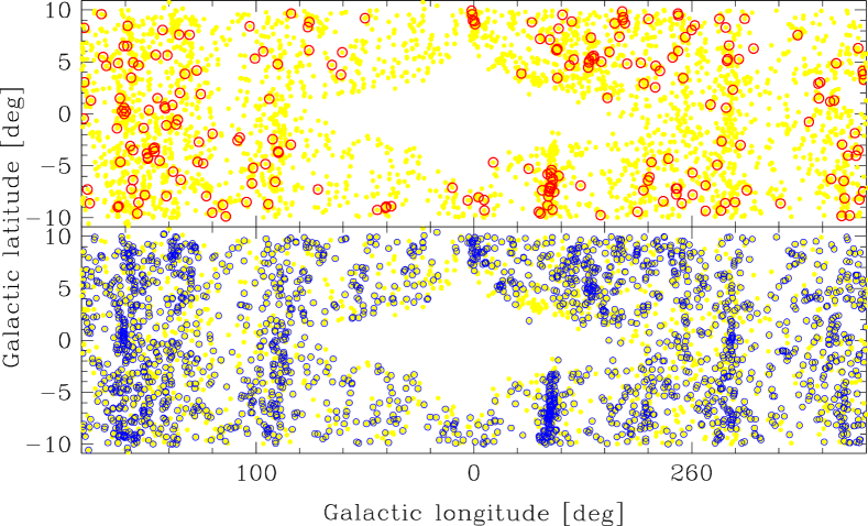
Figure 9: Comparison of the sky distributions of ZOA galaxies with and without a discernible disc in the NIR. All galaxies are indicated by yellow dots. Top panel: Galaxies with a D4 classification (i.e., no visible disc) are shown as red circles. Bottom panel: Galaxies with a D1 classification (i.e., with a clear disc) are shown as blue circles.

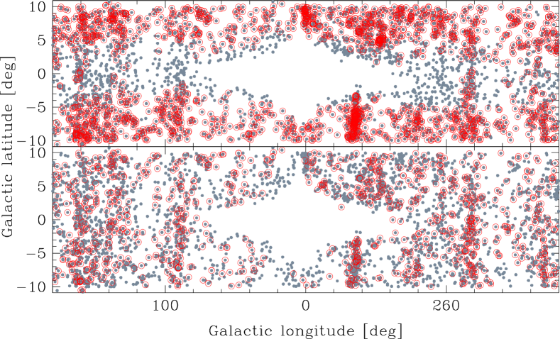
Figure 10: Sky distributions of ZOA galaxies with or without known redshifts. All galaxies are indicated by grey dots; red circles indicate objects with redshift measurements. The top panel shows optical redshift measurements ($N=2241$), the bottom panel H I detections ($N=963$).

In Fig. 9 we show the sky distribution of the two extreme classifications, $D4$ (no disc, red circles in top panel) and $D1$ (clear disc, blue circles in bottom panel). In the case of $D4$ (which basically stands for elliptical galaxies) we would expect to see the cores of rich clusters, and indeed we can discern, for example, the Norma cluster (Abell 3627, $l\simeq 325\degr$, $b\simeq-7\degr$), the Ophiuchus Cluster ($l\simeq 0\degr$, $b\simeq 9\degr$) and the cluster around 3C129 ($l\simeq 160\degr$, $b\simeq 0\aas@@fstack{\circ}5$) which was revealed to be a rich cluster through our NRT observations (Paper II) and the follow-up observations with the Westerbork Synthesis Radio Telescope (Ramatsoku et al., 2014, 2016).

As there are about nine times more galaxies classified as $D1$ (clear disc, that is, spiral galaxies) the bottom panel is more crowded, revealing more filamentary structures, predominantly in the N-S direction: e.g., the Puppis filament at $l\simeq 245\degr$, as well as the western and eastern arm of the Perseus-Pisces filament ($l\simeq 160\degr$ and $l\simeq 90\degr$, respectively; see Ramatsoku et al. 2014, Paper II).

5.5 Radial velocity information

For 2620 galaxies (70%; with 2549 in the ZOA sample) we have found at least one radial velocity measurement in the literature. For a further 293 (279) galaxies, redshifts will be publicly available presently: six are optical measurements (from the updated 2MRS catalogue); the H I measurements are mainly from our observing campaigns at Nançay and Parkes (see Sec. 2.2 for details). This will increase the total number of galaxies with at least one redshift measurement to 2805 (2729). All redshifts will be presented in a forthcoming paper in combination with an analysis of the whole-sky redshift distribution.

When we plot the distribution of these galaxies on the sky and distinguish between optical and H I redshifts (see the red circles in the upper and lower panels, respectively, of Fig. 10), two features are immediately obvious: (i) the inner ZoA is dominated by H I detections, and (ii) the H I detections, unlike the optical detections, do not show pronounced clustering (Koribalski et al., 2004). Both effects are typical for the respective types of measurement.

We show the number densities of galaxies in the ZOA sample with and without velocity information as a function of stellar density and extinction $A_{\rm K}$ in Fig. 11 (top and bottom panel, respectively) using the same method as for Fig. 7. As before, the extinction histogram has been restricted to areas with stellar densities $\log N_{*}/{\rm deg}^{2}<4.5$. Though we would expect the number density of galaxies with H I measurements (magenta; $N=963$) not to show any dependence on either stellar density or extinction, we find a slight drop-off in both histograms. This is understandable since most H I observations in the north are from pointed observations of recognisable galaxies in lower-stellar density environments; only one (shallow) blind survey exists so far, i.e., EBHIS (Kerp et al., 2011). On the other hand, number densities of galaxies with optical measurements (green; $N=2241$) show, as expected, a strong decrease with extinction, but also a dependence on stellar densities. This is partially due to the fact that many of the optical measurements have been obtained by the 2MRS collaboration and thus are restricted to higher latitudes where both extinction and stellar densities are lower. Note that for 475 galaxies both kinds of velocity measurements are available. For completeness, we also show galaxies without any velocity information (black; $N=946$).

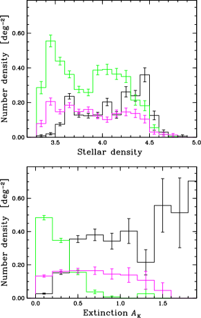
Figure 11: Histograms of the number density of ZOA sample galaxies with optical redshifts (green), H I redshifts (magenta) and no velocity information at all (black). Top panel: as a function of stellar density; bottom panel: as a function of Galactic $A_{\rm K}$ (only regions with $\log N_{*}/{\rm deg}^{2}\leq 4.5$ were used). Poissonian errors per bin are indicated with error bars.

5.6 2MASS parameters

Throughout the following analysis we have excluded all galaxies which have a photometry or extinction flag set, or for which $A_{\rm K}>3\aas@@fstack{m}0$. Unless stated otherwise, we used the combined ZOA & EBV catalogue. Histograms were normalised by total number in the regarded sample.

5.6.1 Diameters and magnitudes

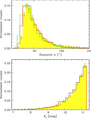
Figure 12: Normalised histograms of major axis diameters in arcseconds (top) and $K_{\rm s}$-band magnitudes (bottom panel) for 2MASX galaxies. Yellow histograms represent the average high Galactic latitude sample; green histograms are for the combined ZOA & EBV galaxy sample (where the $K_{\rm s}$- band magnitude is corrected for Galactic foreground extinction, $K^{\rm o}_{\rm s}$); red histograms are the same but with the additional, diameter-dependent extinction applied ($a^{\rm d}$ and $K^{\rm o,d}_{\rm s}$).

Figure 12 shows the normalised histograms of the parameters major axis diameter $a$ (top panel) and $K_{\rm s}$-band magnitude (bottom panel) for various samples. First, we compare the parameters of our sample (green lines, with magnitudes corrected for foreground extinction, i.e., $K^{\rm o}_{\rm s}$), with those corrected for the diameter-dependent extinction (see Sec. 3.3), $a^{\rm d}$ and $K^{\rm o,d}_{\rm s}$ (red lines). We find that while the diameters $a^{\rm d}$ show a clear shift to larger values compared to $a$ (as expected), there is no obvious similar shift towards brighter $K_{\rm s}$-band magnitudes.

Table 5: Statistics on 2MASX parameters of various samples

Parameter (sample)	$N^{*}$	min	max	median	error
Diameter:
$a$ (comb${\dagger}$)	3365	$15\aas@@fstack{\prime\prime}0$	573″	$41\aas@@fstack{\prime\prime}2$	0.5
$a^{\rm d}$(comb${\dagger}$)	3301	$17\aas@@fstack{\prime\prime}5$	273″	$43\aas@@fstack{\prime\prime}6$	0.4
$a$ (high-lat‡)	$2950-3374$	$13\aas@@fstack{\prime\prime}6$	1260″	$45\aas@@fstack{\prime\prime}8-49\aas@@fstack{\prime\prime}6$	$0.4-0.9$
$a^{\rm d}$ (ext’d§)	3344	$17\aas@@fstack{\prime\prime}3$	273″	$43\aas@@fstack{\prime\prime}4$	0.4
$K_{\rm s}$-band magnitude:
$K^{\rm o}_{\rm s}$(comb${\dagger}$)	3365	$4\aas@@fstack{m}32$	$11\aas@@fstack{m}25$	$10\aas@@fstack{m}74$	0.01
$K^{\rm o,d}_{\rm s}$(comb${\dagger}$)	3301	$6\aas@@fstack{m}78$	$11\aas@@fstack{m}25$	$10\aas@@fstack{m}74$	0.01
$K_{\rm s}$ (high-lat‡)	$2950-3374$	$1\aas@@fstack{m}55$	$11\aas@@fstack{m}25$	$10\aas@@fstack{m}72-10\aas@@fstack{m}78$	$0.01-0.02$
$K^{\rm o,d}_{\rm s}$ (ext’d§)	3344	$6\aas@@fstack{m}78$	$11\aas@@fstack{m}25$	$10\aas@@fstack{m}75$	0.01
∗ sample size; † combined ZOA and EBV sample;             ‡ high-latitude sample; § extended sample

To assess whether the diameter-dependent extinction correction is adequate, we compared our sample parameters with those of galaxies well outside the ZoA. We extracted two samples of 2MASX galaxies from high latitudes ($|b|>30\degr$) with the same magnitude limit of $K_{\rm s}$$<11\aas@@fstack{m}25$ (uncorrected for foreground extinction). The samples contain $6747$ objects from the northern Galactic cap and $5900$ from the southern Galactic cap. As these numbers are affected by cosmic variance, we used a simplistic method to represent this effect by extracting 12 subsamples from the total sample, each with $\sim\!3000$ galaxies selected using different criteria (either random or by sorting in RA). We then took the mean of these normalised histograms and determined the scatter in each bin. The result is shown as the yellow filled (averaged) histograms in Fig. 12, where the black error bars represent the scatter in those bins.

To quantify the results, Table 5 gives sample size $N$, the minimum and maximum values as well as median values for the different samples. We decided to use the median values for the comparison since the histograms are skewed, and we cannot apply the KS-test. As an estimate for the uncertainties we list the errors in the mean (which compare reasonably well with the dispersion in the median of the high-latitude samples).

As already noticed in Fig. 12, the median value of the diameters of our sample shows a clear shift from uncorrected, $a$, to corrected diameters, $a^{\rm d}$, by $\sim\!6\sigma$. However, all high-latitude samples have diameters even larger by at least $5\sigma$ compared to our $a^{\rm d}$, and by $8\sigma$ compared to the median value of the full high-latitude sample ($N=12,647$), $47\aas@@fstack{\prime\prime}0$. This suggests that the diameter-dependent extinction correction as derived by Riad et al. (2010) is too conservative and not quite sufficient for our sample. A selection bias with respect to size as an alternative explanation is unlikely because we select on magnitudes which show no difference (see discussion below).

In case of the $K_{\rm s}$-band magnitudes, in the ZoA the median $K^{\rm o,d}_{\rm s}$ magnitude is the same as the median $K^{\rm o}_{\rm s}$ magnitude, and both lie well within the range of median values found for the high-latitude samples. It is important to note, though, that with the diameter-dependent correction our sample cut-off at $K^{\rm o}_{\rm s}$$=11\aas@@fstack{m}25$ no longer results in a complete sample since we lack those galaxies which are fainter than $K^{\rm o}_{\rm s}$ but have $K^{\rm o,d}_{\rm s}$$\leq 11\aas@@fstack{m}25$. We therefore extended our sample by (a) adding the supplementary $K^{\rm o,d}_{\rm s}$-sample described in the appendix (with a new magnitude cut at $K^{\rm o,d}_{\rm s}$$=11\aas@@fstack{m}25$; see also Sec. 3.3) and (b) excluding other galaxies where the reduced extinction correction due to the SF11 factor 0.86 makes them fainter than our magnitude limit (see appendix) so that we again have a complete magnitude-limited sample (called the extended sample in Table 5). We find that the median $K^{\rm o,d}_{\rm s}$ magnitude of $10\aas@@fstack{m}75$ for this extended sample is comparable to the previous values. This is expected because there are two, opposing, corrections which almost cancel each other out: the diameter-dependent extinction correction makes magnitudes brighter, whereas the correction factor $f=0.86$ (SF11), which is also applied when deriving $K^{\rm o,d}_{\rm s}$ values, makes magnitudes fainter.

On the other hand, the median extinction corrected diameter $a^{\rm d}$ of this extended sample is slightly smaller than previously and compared to the high-latitude samples it is significantly smaller by $\sim\!9\sigma$.

As a sanity check on whether the enforced cut-off has an influence on the median we did the same tests on a diameter-limited subsample using a lower diameter limit of 40 arcseconds. The results confirmed the above findings.

It thus seems that the diameter-dependent extinction correction for the diameter is not sufficient and that intrinsically the galaxies in the ZoA are likely to be larger (by $\sim\!4\arcsec$). The diameter-dependent extinction correction for the $K_{\rm s}$-band magnitudes is not affected by this underestimation since the magnitude correction is independent of the actual diameter of a galaxy (Cameron, 1990).

5.6.2 NIR colours

The normalised histograms for the colours $(J-K_{\rm s})$ and $(H-K_{\rm s})$ are shown in Fig. 13. As for Fig. 12, the green histograms show the extinction-corrected colours ($(H-K_{\rm s})^{\rm o}$ and $(J-K_{\rm s})^{\rm o}$) of our sample, while the yellow filled histograms are the average of the high-latitude samples (where no extinction correction has been applied). As explained in Sec. 3.3, the colours are not affected by the diameter-dependent extinction correction though we did apply the correction factor 0.86 (SF11) to the $E(B-V)$ values used in the extinction correction; these colours are shown as red histograms (designated as $(H-K_{\rm s})^{\rm o,c}$ and $(J-K_{\rm s})^{\rm o,c}$).

Although the scatter in the colours is large since they are sensitive to problems with extinction and photometry, the mean values are well defined: $<(J-K_{\rm s})^{\rm o}>=0\aas@@fstack{m}938\pm 0\aas@@fstack{m}002$ and $<(H-K_{\rm s})^{\rm o}>=0\aas@@fstack{m}279\pm 0\aas@@fstack{m}002$ with a standard deviation of $\pm$$0\aas@@fstack{m}13$ and $\pm$$0\aas@@fstack{m}08$, respectively. These values are both bluer than those of the full high-latitude sample ($1\aas@@fstack{m}013\pm 0\aas@@fstack{m}001$ and $0\aas@@fstack{m}302\pm 0\aas@@fstack{m}001$, respectively). The application of the improved extinction correction as recommended by SF11, however, changes the mean colours to $0\aas@@fstack{m}988$ and $0\aas@@fstack{m}296$, respectively, which is in good agreement with the high-latitude samples. We summarise the statistics of the various samples in Table 6 where we give the sample size $N$, the mean and its error, as well as the standard deviation (or scatter) of the samples.

Jarrett (2000) and Jarrett et al. (2003) present NIR colours as a function of morphological type: for early-type spirals they find a $(J-K_{\rm s})$ value comparable to ours, that is, $\sim\!1\aas@@fstack{m}0$, while their $(H-K_{\rm s})$ colour is bluer: $0\aas@@fstack{m}27$. Later type spirals are generally bluer. The comparison, though, is affected on the one hand by the small sample size in the large galaxy catalogue (Jarrett 2000, where the total sample consists of 100 galaxies), and on the other hand by our sample including galaxies at larger redshifts which appear redder (though the contamination by these is constrained by our bright magnitude cut-off).

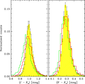
Figure 13: Normalised histograms of 2MASX colours $(J-K_{\rm s})$ (left) and $(H-K_{\rm s})$ (right). Yellow histograms represent the average high Galactic latitude sample; green histograms are the combined ZOA & EBV galaxy sample (corrected for Galactic foreground extinction); red histograms are the latter sample but with the SF11 correction factor 0.86 used in the extinction correction.

Table 6: Statistics on 2MASX colours of various samples

Sample	$(J-K_{\rm s})$				$(H-K_{\rm s})$
	$N^{*}$	mean	error	standard deviation	$N^{*}$	mean	error	standard deviation
		[mag]	[mag]	[mag]		[mag]	[mag]	[mag]
Colouro  (comb†)	3255	$0.938$	$0.002$	$0.13$	3322	$0.279$	$0.001$	$0.08$
Colouro,c  (comb†)	3255	$0.988$	$0.002$	$0.12$	3322	$0.296$	$0.001$	$0.07$
Colour  (high-lat‡)	$2939-3372$	$1.000-1.022$	$0.002-0.003$	$0.10-0.19$	$2939-3372$	$0.294-0.313$	$0.001-0.002$	$0.07-0.13$
Colouro  (comb, corr§)	3220	$0.962$	$0.002$	$0.13$	3287	$0.293$	$0.001$	$0.08$
Colouro,c  (comb, corr§)	3220	$1.012$	$0.002$	$0.12$	3287	$0.310$	$0.001$	$0.08$
∗ sample size; † combined ZOA and EBV sample; ‡ high-latitude sample; § combined ZOA and EBV sample corrected for stellar density dependence

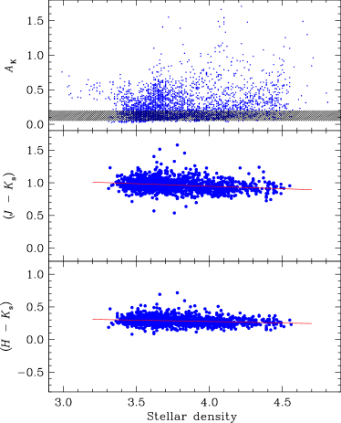
Figure 14: Top panel: Galactic extinction $A_{\rm K}$ as a function of stellar density for our galaxy sample. The shaded area indicates the range of $0\aas@@fstack{m}05<A_{\rm K}<0\aas@@fstack{m}2$ where the stellar density and extinction are not correlated (see text). Middle panel: colour $(J-K_{\rm s})^{\rm o}$ as a function of stellar density, for the sample defined by the shaded area in the top panel. Bottom panel: same for the $(H-K_{\rm s})^{\rm o}$ colour. The red lines show the linear fits to the distributions.

As we have shown above, some properties of ZoA galaxies are not only affected by Galactic foreground extinction but also by stellar density. Since there is a large overlap between regions with high stellar densities and with high Galactic extinction (see Fig. 6), we need to find a subsample where the Galactic extinction and stellar densities are not correlated. Based on Fig. 14, which shows the extinction values as a function of stellar density for our sample (top panel), we have chosen the range of $0\aas@@fstack{m}05<A_{\rm K}<0\aas@@fstack{m}2$ (shaded area in the plot) where there is no obvious dependence on stellar densities. For this subsample of 1395 galaxies we find a dependence of the colours $(J-K_{\rm s})^{\rm o}$ and $(H-K_{\rm s})^{\rm o}$ on stellar density (see middle and bottom panel, respectively). Linear fits to both relationships give

$$(J-K_{\rm s})^{\rm o}=(-0.078\pm 0.009)\cdot\log N_{*}/{\rm deg}^{2}+(1.258\pm 0.036)$$

and

$$(H-K_{\rm s})^{\rm o}=(-0.043\pm 0.006)\cdot\log N_{*}/{\rm deg}^{2}+(0.449\pm 0.024).$$

Incidentally, the slopes in these relationships vary only marginally if we chose a different extinction range for the subsample (e.g., increasing the upper limit up to $A_{\rm K}=0\aas@@fstack{m}5$). Applying these mean relationships as a correction to the original sample (and using $\log N_{*}/{\rm deg}^{2}=3.5$ as reference point) we obtain colours independent of stellar density, that is, $<(J-K_{\rm s})^{\rm o}>=0\aas@@fstack{m}962\pm 0\aas@@fstack{m}002$ and $<(H-K_{\rm s})^{\rm o}>=0\aas@@fstack{m}293\pm 0\aas@@fstack{m}001$ as well as $<(J-K_{\rm s})^{\rm o,c}>=1\aas@@fstack{m}012\pm 0\aas@@fstack{m}002$ and $<(H-K_{\rm s})^{\rm o,c}>=0\aas@@fstack{m}310\pm 0\aas@@fstack{m}001$ (listed as the combined and corrected sample in Table 6). The latter two are in excellent agreement with the high-latitude sample. The shapes of the distributions of the fully-corrected colours agree as well (though this is not shown in Fig. 13 to avoid confusion). We conclude that at high stellar densities, where the likelihood of unsubtracted or undetected faint stars affecting the galaxy photometry is higher, galaxy colours are too blue and thus not reliable. For example, at the highest stellar densities where we still detect galaxies, $\log N_{*}/{\rm deg}^{2}=4.5$, the $(J-K_{\rm s})^{\rm o}$ and $(H-K_{\rm s})^{\rm o}$ colours are too blue by $0\aas@@fstack{m}08$ and $0\aas@@fstack{m}04$, respectively.

Since galaxy colours are sensitive to foreground extinction, they in turn can be used to investigate the foreground extinction in more detail (Schröder et al., 2007). We will revisit this in a forthcoming paper (Paper III).

6 Summary and discussion

In this first of a series of papers, we presented a magnitude-limited catalogue of 2MASX galaxies at low Galactic latitudes and at high foreground extinction levels. The catalogue supplements the high-latitude 2MRS (Huchra et al., 2012) and 2MTF (e.g., Masters et al. 2014) surveys with the aim to obtain a homogeneous, complete and truly ‘whole-sky’ survey for cosmic flow analyses (the forthcoming papers will address these aims). We have used an extinction-corrected magnitude limit of $K^{\rm o}_{\rm s}$$=11\aas@@fstack{m}25$ which is brighter than the 2MRS limit of $K^{\rm o}_{\rm s}$ $=11\aas@@fstack{m}75$, but the higher extinctions in our sample would make the parameters of fainter galaxies less reliable. At all Galactic longitudes, we extracted 2MASX objects with latitudes $|b|<10\degr$ (the ‘ZOA sample’) and at higher latitudes we selected all objects with $E(B-V)$$>0\aas@@fstack{m}950$ (the ‘EBV sample’). All objects were visually inspected across a wide wavelength range to exclude all non galaxies from the sample. This results in 3675 and 88 galaxies in the ZOA and EBV galaxy sample, respectively, with a rejection rate for non-galaxies in the 2MASX catalogue of 47% and 82%, respectively. The completeness of our catalogue is mainly affected by the stellar density (the completeness limit lies at $\log N_{*}/{\rm deg}^{2}=4.5$), while the extinction seems to have only a small effect, if any, up to $A_{\rm K}\simeq 2\aas@@fstack{m}0$. Thus, the NIR ZoA for bright galaxies covers only 2.4% of the full sky. For each galaxy we give an estimate of its morphological type, based on the likelihood of it having a disc. Furthermore, we identified which galaxies have optical or H I radial velocities measurements.

Since the uncertainties in galaxy parameters increase towards the Galactic plane, we discuss the effects of foreground extinction and high stellar densities. In particular, the 2MASX photometry in the ZoA is affected by the high stellar densities which (i) increase the confusion noise and therewith decrease the sensitivity which can bias the background subtraction (Jarrett et al., 2000), (ii) can cause the centre of the extraction aperture to be located on a superimposed star instead of the galaxy, and (iii) sometimes affects the size, ellipticity and position angle of the extraction aperture. Based on investigations by Said et al. (2016), Andreon (2002) and Kirby et al. (2008), we conclude that 2MASX magnitudes in the ZoA are on average too bright by at least $0\aas@@fstack{m}35$ compared to 2MASX galaxies at higher latitudes, an effect which needs to be taken into account when combining the 2MRS and 2MTF surveys with our catalogue. The colours as well are sensitive to unresolved stars in the field, and we show that at the high stellar density level of $\log N_{*}/{\rm deg}^{2}=4.5$ the colours $(J-K_{\rm s})^{\rm o}$ and $(H-K_{\rm s})^{\rm o}$are too blue on average by $0\aas@@fstack{m}08$ and $0\aas@@fstack{m}04$, respectively. We estimate the uncertainty in the limiting magnitude of $11\aas@@fstack{m}25$ of our catalogue to be $\sim\!0\aas@@fstack{m}15$.

Considering the problems of obtaining accurate photometry in star-crowded areas as well as the underestimation of the 2MASX fluxes due to the short exposure time, we strongly argue for deeper all-sky surveys with higher spatial resolution in the NIR. These will be available for the southern hemisphere once the VHS (McMahon et al., 2013) and VVV (Minniti et al., 2010) surveys are fully completed, but not in the north where the UKIRT Hemisphere Survey (Dye et al., 2018) does not cover the North Celestial Cap.

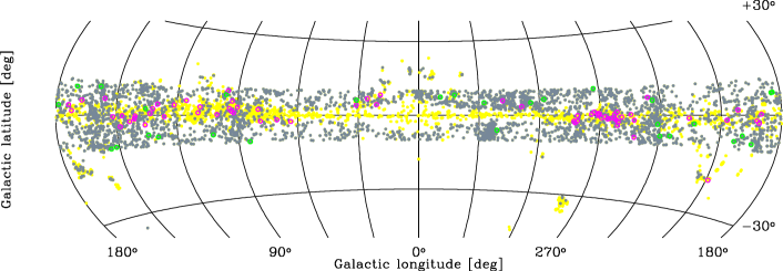
Figure 16: Aitoff projection of the distribution on the sky of the objects in the main, supplementary and exclusion samples, in Galactic coordinates. Yellow dots represent non-galaxian objects, grey dots galaxies from the main catalogue, magenta circles supplementary sample galaxies and green circles exclusion sample galaxies.

Different kinds of Galactic extinction corrections are suggested in the literature: values extracted from DIRBE/IRAS maps by SFD98 were found to be too high and need to be corrected (e.g., Schröder et al. 2007; Schlafly & Finkbeiner 2011). In addition, the measured size of an obscured galaxy is also affected by foreground extinction, and an additional correction for the isophotal diameter is necessary (Cameron 1990, Riad et al. 2010). While the sample selection of our main catalogue is based on the SFD98 correction, so as to be as close as possible to the selection criteria of the 2MRS survey, we also include the optimal extinction correction to the photometry parameters in our catalogue and discussion. We also investigated how the sample selection would change if this optimal extinction correction were applied: Firstly, because the diameter-dependent extinction correction makes a galaxy brighter, we additionally extracted all the 2MASX objects which are brighter than the fully corrected magnitude limit of $K^{\rm o,d}_{\rm s}$$=11\aas@@fstack{m}25$, but are fainter than our original limit of $K^{\rm o}_{\rm s}$$=11\aas@@fstack{m}25$. This supplementary sample comprises 70 and 1 additional galaxies in the ZOA and EBV samples, respectively. Secondly, 29 and 0 galaxies, respectively, are removed from the catalogue due to the SF11 correction factor to the extinction values. While these two effects almost cancel each other out and the so-called supplementary sample is small, it is nonetheless an important correction to the main catalogue and should be taken into account in any flow field analyses to avoid biases due to the patchy distribution of the supplementary galaxies (see Figure 16 in the appendix).

For a truly unbiased analysis, the 2MRS and 2MTF photometry needs to have the same correction applied. To emphasise the importance of this correction we show in Fig. 15 the histograms of the additional correction due to the diameter-dependent extinction correction for all 2MRS galaxies in our two samples. Note that for an unbiased comparison, we applied the SF11 correction factor, $f=0.86$, to the $K^{\rm o}_{\rm s}$ values (now denoted as $K^{\rm o,c}_{\rm s}$).

For the ZOA sample the median difference in magnitude is $0\aas@@fstack{m}02$, where 34 galaxies (1.4% out of 2360) deviate more than $0\aas@@fstack{m}10$. For the EBV sample, that is, in the overlap region of $E(B-V)$  $=0\aas@@fstack{m}950-1\aas@@fstack{m}000$, we have a median difference of $0\aas@@fstack{m}07$, and 14 out of the 72 galaxies (19%) deviate more than $0\aas@@fstack{m}10$. Though the numbers and areas affected by extinctions above $0\aas@@fstack{m}95$ are small, the omission of this correction even even a much lower level of, for example, $E(B-V)$$=0\aas@@fstack{m}44$ (or $A_{\rm K}=0\aas@@fstack{m}16$) would imply a systematic error in magnitude of the order of the typical uncertainty in galaxy magnitudes, that is, $0\aas@@fstack{m}20$. Such a magnitude difference would result in distances 10% too large, and could affect peculiar velocities by as much as a factor of 2. And since the foreground extinction is distributed unevenly across the sky this bias could mimic a non-existent flow field (e.g., Kolatt et al. 1995).

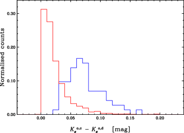
Figure 15: Histograms of the difference between $K_{\rm s}$-band magnitudes after basic extinction correction using the SF11 correction factor $f=0.86$, $K^{\rm o,c}_{\rm s}$, and magnitudes with the additional diameter correction, $K^{\rm o,d}_{\rm s}$, for the ZOA sample (red) and EBV sample (blue); only galaxies that are also in the 2MRS catalogue are shown.

We also find that the value of the foreground extinction for a given galaxy can be uncertain, especially in high extinction areas of molecular clouds, as it is based on the relatively coarse $6\arcmin$-resolution of the DIRBE/IRAS maps. In addition, at $|b|<5\degr$ no FIR sources were subtracted from these maps due to confusion problems. In this region, we find three bright FIR sources that clearly bias the local extinction estimates. We estimate that a further $\lower 1.99997pt\hbox{$\buildrel>\over{\sim}$}\,22$% of the galaxies are likely affected by weaker FIR sources. This effect needs to be taken into account in cosmic flow analyses since it implies that extinction-corrected magnitudes of affected galaxies will be systemically too bright, albeit by a small amount. We have flagged both effects in the catalogue.

To ensure that a combination of our catalogue with the 2MRS and 2MTF surveys will not introduce a bias, we compare the extinction-corrected 2MASX diameter and $K_{\rm s}$-band magnitude of our galaxies with a high-latitude 2MASX galaxy sample with the same magnitude limit. While the median values of the $K_{\rm s}$-band magnitude agree well within the errors, the diameters in the ZoA are systematically too small by $\sim 4^{\prime\prime}$ even when we apply the diameter-dependent extinction correction. We assume this is likely due to an incomplete diameter-dependent extinction correction which was derived from a small sample (Riad et al., 2010). Since no such effect for the corrected magnitudes could be found, we are confident that the sample selection, which is based on magnitudes, is not affected.

Finally, we find that although the galaxy extraction from the 2MASX catalogue presented here is complete to a given limit in magnitude, the catalogue itself is missing galaxies in the Galactic bulge area due to the difficulties of the 2MASX automated galaxy-star separation algorithms to identify galaxies in regions of high stellar density. NIR surveys with a better spatial resolution can help reduce the remaining ZoA (e.g., Vista-VVV, Minniti et al. 2010, and UKIDSS-GPS, Lucas et al. 2008), in particular in conjunction with improved galaxy detection algorithms (based on machine learning, e.g., González et al. 2018).

To further improve the sample we propose to use a semi-automated script to extract better (2MASS) galaxy photometry (e.g., Said 2017) and thus remove some of the uncertainties in the magnitude limit of the sample (or sample definition). Furthermore, we find that galaxy photometry in the ZoA not only requires a correction for Galactic extinction but also that the increased confusion noise (due to unresolved faint stars) affects the accuracy of the background subtraction. For example, at high latitudes the 20 mag arcsec^-2 isophotal $K_{\rm s}$-band magnitude corresponds roughly to only $1\sigma$ of the typical background noise in the $K_{\rm s}$-band (Jarrett et al., 2000), but at low latitudes the increased noise level means that the isophotal aperture is less well determined. Thus, all photometry used in cosmic flow field analyses should preferentially be derived from NIR observations deeper than 2MASX (e.g., UKIDSS or VISTA survey data).

To conclude, a recipe for combining high-latitude surveys like 2MRS and 2MTF with a ZoA survey like ours needs to address the following issues: (a) full extinction corrections need to be applied in the same manner to all galaxies, even at moderate extinction levels; (b) possible offsets in the isophotal magnitudes due to increased background noise in the Galactic plane need to be corrected for; (c) the variance in photometric quality and thus the increased photometric uncertainties in localised areas on the sky needs to be understood and taken into account as a possible bias; (d) over-estimation of the extinction correction for a significant number of galaxies due to weak and unresolved FIR sources in the IRAS/DIRBE maps at low latitudes need to be assessed and taken into account.

In the forthcoming papers we will present H I observations for those galaxies that do not yet have redshifts and of those with redshifts that are eligible for the TF analysis. Preparatory work on the application of the TF relation in the ZoA has been done by Said et al. (2015), who determined that isophotal apertures are less affected by high stellar densities than total magnitudes, and that axial ratios need to be corrected for extinction. The final paper in this series will deal with the application the TF relation to the whole-sky sample (see Said 2017 for a pilot study). Fine-tuning of the Galactic foreground extinction determination will be discussed in another paper in this series (Schröder et al., in prep.).

Appendix A Extended catalogue according to optimised extinction corrections

In Sec 3.3 we discuss an additional Galactic foreground extinction correction for isophotal radii and thus isophotal magnitudes. The main catalogue includes photometry parameters based on this additional correction as well as a recommended correction to the $E(B-V)$ values from the IRAS/DIRBE maps (SF11; Sec. 3.2). Since the magnitudes are affected, the sample selection criterion regarding a limiting magnitude is not ful-filled anymore. Hence, we investigated how the sample selection would change if this optimal extinction correction were applied and thus compiled an ‘extended’ catalogue.

Any extinction correction makes galaxy magnitudes brighter. If we apply a diameter-dependent extinction correction in addition to the conventional Galactic foreground extinction correction, the magnitude limit of our sample, $K^{\rm o}_{\rm s}$ $=11\aas@@fstack{m}25$ is not longer valid and the sample becomes incomplete. We therefore need to supplement our catalogue by adding all those galaxies with $K^{\rm o}_{\rm s}$$>11\aas@@fstack{m}25$ but $K^{\rm o,d}_{\rm s}$$\leq 11\aas@@fstack{m}25$. The supplementary sample which contains these galaxies is presented in Table LABEL:zoaihabtabex (available online) with the same columns as for the main catalogue (see Sec. 4). It comprises 276 and 14 additional objects for the ZOA and EBV samples, respectively. Applying the object flags we devised for classifying sources as galaxies (Table LABEL:zoatabex, Col. 4) results in 70 and 1 additional galaxies, respectively.

On the other hand, galaxies will be excluded from the main catalogue since in the derivation of the optimally extinction-corrected $K^{\rm o,d}_{\rm s}$ values we applied the correction factor 0.86 from SF11 to the $E(B-V)$ values used, which makes magnitudes fainter. Objects thus excluded from the main catalogue are flagged (Table LABEL:zoatabex, Col. 7d). For ease of use, we repeat those lines in Table LABEL:zoaexcltab (dubbed the exclusion sample). There are 31 and 1 objects affected in the ZOA and EBV samples, respectively, of which 29 and 0 are galaxies. In total there are 3716 and 89 galaxies in the ‘extended’ ZOA and EBV samples, respectively, using $K^{\rm o,d}_{\rm s}$ $=11\aas@@fstack{m}25$ (as opposed to the original 3675 and 88, respectively).

Compared to the main catalogue, the supplementary sample has considerably fewer matches in the 2MRS catalogue: only 4 objects (1%) have a 2MRS counterpart. This is expected as the former includes objects fainter than the 2MRS cut-off at $K_{\rm s}$$\leq 11\aas@@fstack{m}75$. Another characterisation of a sample with fainter objects is the greater uncertainty in galaxy classification (in particular in our classes 4, 5 and 6), and disc types (uncertain class, D3, and unknown, ‘n’). This is in fact one of the reasons why we prefer a higher magnitude limit for our sample, that is, $11\aas@@fstack{m}25$ versus $11\aas@@fstack{m}75$ as used by the 2MRS project. Finally, in the supplementary sample only 6% galaxies have published redshifts (versus 70% in the main catalogue).

Figure 16 shows the distribution on the sky of the supplementary galaxies (magenta circles), which is patchy and more concentrated towards the Galactic plane compared to the main catalogue galaxies (grey dots). Galaxies excluded from the main catalogue are shown in green.

Table 7: 2MASS ZoA supplementary sample; example page, the full table is available online

2MASX J	$l$	$b$	EBV	Object			Sample				Disc	2MRS	Velocity		NIR	Photom	Ext	$K_{20}$	$H$-$K$	$J$-$K$	vc	$a$	$b/a$	st.d.	$K^{\rm o}_{\rm s}$	($H$-$K)^{o}$	($J$-$K)^{o}$	$A_{\rm K}$	$a^{\rm d}$	$K^{\rm o,d}_{\rm s}$	($H$-$K)^{o,c}$	($J$-$K)^{o,c}$
	deg	deg	mag	class	off	flg	gal	TF	obs	ext’d	type		Opt	HI	flg	flg	flg	mag	mag	mag		”			mag	mag	mag	mag	′′	mag	mag	mag
(1)	(2a)	(2b)	(3)	(4)	(5)	(6)	(7a)	(7b)	(7c)	(7d)	(8)	(9)	(10a)	(10b)	(11)	(12)	(13)	(14)	(15)	(16)	(17)	(18)	(19)	(20)	(21)	(22)	(23)	(24)	(25)	(26)	(27)	(28)
00012132$+$6706042	118.077	$4.703$	$4.827$	6	$-$	$-$	$-$	$-$	$-$	$-$	$-$	$-$	$-$	$-$	$-$	$-$	e	$13.262$	$\cdots$	$\cdots$	$-1$	17.0	$1.00$	$3.79$	$11.463$	$\cdots$	$\cdots$	1.50	$\cdots$	$\cdots$	$\cdots$	$\cdots$
00021688$+$6719539	118.209	$4.912$	$4.737$	8	$-$	$-$	$-$	$-$	$-$	$-$	$-$	$-$	$-$	$-$	$-$	$-$	$-$	$13.232$	$0.57$	$1.65$	$-1$	12.8	$1.00$	$4.13$	$11.467$	$-0.21$	$-0.71$	1.47	$\cdots$	$\cdots$	$-0.12$	$-0.39$
00102080$+$6521098	118.662	$2.822$	$4.784$	7	$-$	$-$	$-$	$-$	$-$	$-$	$-$	$-$	$-$	$-$	$-$	$-$	$-$	$13.118$	$1.10$	$1.61$	$-1$	17.6	$1.00$	$3.83$	$11.335$	$0.30$	$-0.77$	1.48	$\cdots$	$\cdots$	$0.40$	$-0.45$
00235245$+$6610283	120.149	$3.452$	$4.307$	7	$-$	$-$	$-$	$-$	$-$	$-$	$-$	$-$	$-$	$-$	$-$	$-$	$-$	$13.105$	$0.77$	$\cdots$	$1$	20.4	$0.54$	$3.86$	$11.500$	$0.06$	$\cdots$	1.33	$\cdots$	$\cdots$	$0.15$	$\cdots$
00235531$+$6605253	120.145	$3.368$	$4.505$	8	$-$	$-$	$-$	$-$	$-$	$-$	$-$	$-$	$-$	$-$	$-$	$-$	$-$	$13.138$	$1.11$	$\cdots$	$1$	17.0	$0.48$	$3.86$	$11.459$	$0.36$	$\cdots$	1.40	$\cdots$	$\cdots$	$0.45$	$\cdots$
00262333$+$6446048	120.265	$2.026$	$4.632$	8	$-$	$-$	$-$	$-$	$-$	$-$	$-$	$-$	$-$	$-$	$-$	$-$	$-$	$13.138$	$\cdots$	$1.60$	$-1$	10.0	$1.00$	$3.90$	$11.412$	$\cdots$	$-0.70$	1.43	$\cdots$	$\cdots$	$\cdots$	$-0.40$
00265579$+$6510278	120.361	$2.425$	$2.480$	6	$-$	$-$	$-$	$-$	$-$	$-$	$-$	$-$	$-$	$-$	$-$	$-$	$-$	$12.253$	$0.74$	$1.86$	$-2$	20.0	$0.76$	$3.81$	$11.329$	$0.33$	$0.63$	0.77	$\cdots$	$\cdots$	$0.38$	$0.80$
00283778$+$6527431	120.564	$2.695$	$2.976$	7	$-$	$-$	$-$	$-$	$-$	$-$	$-$	$-$	$-$	$-$	$-$	$-$	$-$	$12.547$	$1.01$	$2.31$	$1$	23.2	$0.50$	$3.77$	$11.438$	$0.52$	$0.83$	0.92	$\cdots$	$\cdots$	$0.58$	$1.02$
00291882$+$6419524	120.538	$1.563$	$2.850$	9	$-$	$-$	$-$	$-$	$-$	$-$	$-$	$-$	$-$	$-$	$-$	$-$	$-$	$12.456$	$1.12$	$\cdots$	$1$	34.8	$0.78$	$3.87$	$11.394$	$0.65$	$\cdots$	0.88	$\cdots$	$\cdots$	$0.71$	$\cdots$
00353673$+$6618340	121.340	$3.487$	$1.967$	2	$-$	$-$	g	t	$-$	$-$	D2	$-$	$-$	$-$	$-$	$-$	e	$11.988$	$0.62$	$1.77$	$1$	27.2	$0.40$	$3.80$	$11.255$	$0.29$	$0.80$	0.61	$33.8$	$11.22$	$0.33$	$0.93$

Table 7: continued.

Table 8: a) 2MASS exclusion ZoA sample

2MASX J	$l$	$b$	EBV	Object			Sample				Disc	2MRS	Velocity		NIR	Photom	Ext	$K_{20}$	$H$-$K$	$J$-$K$	vc	$a$	$b/a$	st.d.	$K^{\rm o}_{\rm s}$	($H$-$K)^{o}$	($J$-$K)^{o}$	$A_{\rm K}$	$a^{\rm d}$	$K^{\rm o,d}_{\rm s}$	($H$-$K)^{o,c}$	($J$-$K)^{o,c}$
	deg	deg	mag	class	off	flg	gal	TF	obs	ext’d	type		Opt	HI	flg	flg	flg	mag	mag	mag		”			mag	mag	mag	mag	′′	mag	mag	mag
(1)	(2a)	(2b)	(3)	(4)	(5)	(6)	(7a)	(7b)	(7c)	(7d)	(8)	(9)	(10a)	(10b)	(11)	(12)	(13)	(14)	(15)	(16)	(17)	(18)	(19)	(20)	(21)	(22)	(23)	(24)	(25)	(26)	(27)	(28)
01394085$+$5507549	129.846	$-7.091$	$0.319$	1	$-$	$-$	g	t	N	*	D2	c	o	$-$	$-$	$-$	$-$	$11.368$	$0.49$	$1.25$	$1$	33.4	$0.46$	$3.55$	$11.249$	$0.44$	$1.09$	0.10	$34.0$	$11.26$	$0.45$	$1.11$
02010098$+$6337038	130.569	$1.783$	$1.271$	7	$-$	$-$	$-$	$-$	$-$	*	$-$	$-$	$-$	$-$	$-$	$-$	$-$	$11.713$	$1.02$	$2.36$	$1$	16.4	$0.84$	$3.82$	$11.239$	$0.81$	$1.73$	0.39	$\cdots$	$\cdots$	$0.84$	$1.81$
02122164$+$5441091	134.535	$-6.352$	$0.270$	1	$-$	$-$	g	$-$	$-$	*	D4	c	o	$-$	$-$	$-$	$-$	$11.350$	$0.56$	$1.23$	$1$	28.2	$0.78$	$3.56$	$11.249$	$0.51$	$1.09$	0.08	$28.6$	$11.26$	$0.52$	$1.11$
02422242$+$6213323	135.465	$2.084$	$0.525$	1	$-$	$-$	g	$-$	N	*	D3	$-$	$-$	$-$	$-$	$-$	$-$	$11.445$	$0.49$	$1.38$	$1$	23.6	$0.82$	$3.79$	$11.249$	$0.40$	$1.12$	0.16	$24.4$	$11.26$	$0.41$	$1.15$
03223065$+$6329185	138.871	$5.394$	$1.654$	9	$-$	$-$	$-$	$-$	$-$	*	$-$	$-$	$-$	$-$	$-$	$-$	$-$	$11.854$	$1.63$	$3.21$	$1$	16.6	$0.58$	$3.63$	$11.238$	$1.35$	$2.39$	0.51	$\cdots$	$\cdots$	$1.39$	$2.50$
03351760$+$4401160	151.492	$-9.578$	$0.313$	1	$-$	$-$	g	t	N	*	D2	c	o	$-$	$-$	$-$	$-$	$11.364$	$0.33$	$1.16$	$1$	34.8	$0.44$	$3.53$	$11.247$	$0.28$	$1.00$	0.10	$35.4$	$11.26$	$0.28$	$1.02$
03460109$+$4201053	154.307	$-9.976$	$0.317$	1	$-$	$-$	g	$-$	$-$	*	D2	c	o	$-$	$-$	$-$	$-$	$11.366$	$0.31$	$1.14$	$1$	29.0	$0.78$	$3.46$	$11.248$	$0.26$	$0.99$	0.10	$29.5$	$11.26$	$0.26$	$1.01$
05231302$+$5112435	158.869	$8.400$	$0.389$	1	$-$	$-$	g	$-$	$-$	*	D1	c	o	$-$	$-$	$-$	$-$	$11.389$	$0.31$	$1.19$	$1$	31.0	$0.90$	$3.52$	$11.244$	$0.25$	$1.00$	0.12	$31.8$	$11.25$	$0.26$	$1.02$
05454092$+$1306184	193.613	$-8.158$	$0.507$	1	$-$	$-$	g	t	$-$	*	D1	c	$-$	h	$-$	$-$	$-$	$11.431$	$0.34$	$1.22$	$1$	34.0	$0.32$	$3.43$	$11.242$	$0.26$	$0.97$	0.16	$35.2$	$11.25$	$0.27$	$1.00$
05540495$+$3127485	178.768	$2.866$	$0.492$	1	$-$	$-$	g	$-$	N	*	D3	$-$	$-$	$-$	U	$-$	$-$	$11.422$	$0.44$	$1.31$	$1$	25.0	$0.72$	$3.68$	$11.239$	$0.36$	$1.07$	0.15	$25.8$	$11.25$	$0.37$	$1.10$
05561062$+$4100185	170.662	$7.979$	$0.344$	1	$-$	$-$	g	$-$	$-$	*	D1	c	o	$-$	$-$	$-$	$-$	$11.372$	$0.41$	$1.20$	$1$	39.2	$0.66$	$3.44$	$11.244$	$0.36$	$1.03$	0.11	$40.0$	$11.25$	$0.36$	$1.05$
06041759$+$0946030	198.807	$-5.843$	$0.436$	1	$-$	$-$	g	$-$	$-$	*	D3	c	o	$-$	$-$	$-$	$-$	$11.412$	$0.42$	$1.30$	$1$	35.2	$0.82$	$3.60$	$11.250$	$0.35$	$1.08$	0.14	$36.3$	$11.26$	$0.36$	$1.11$
06051642$+$0535242	202.616	$-7.631$	$0.442$	1	$-$	$-$	g	t	$-$	*	D1	c	o	$-$	$-$	$-$	$-$	$11.415$	$0.38$	$1.22$	$1$	45.4	$0.50$	$3.52$	$11.250$	$0.31$	$1.00$	0.14	$46.9$	$11.25$	$0.32$	$1.03$
06181338$+$2844455	183.687	$6.120$	$0.566$	1	$-$	$-$	g	$-$	$-$	*	D3	c	o	$-$	$-$	$-$	$-$	$11.455$	$0.42$	$1.28$	$1$	26.6	$0.56$	$3.46$	$11.244$	$0.33$	$1.00$	0.18	$27.6$	$11.26$	$0.34$	$1.04$
06191224$+$2810044	184.303	$6.043$	$0.473$	1	$-$	$-$	g	$-$	$-$	*	D3	c	o	$-$	$-$	$-$	$-$	$11.419$	$0.34$	$1.19$	$1$	28.8	$0.90$	$3.49$	$11.243$	$0.26$	$0.96$	0.15	$29.7$	$11.25$	$0.27$	$0.99$
07003437$-$1020151	223.172	$-2.690$	$0.763$	1	$-$	$-$	g	$-$	N	*	D1	$-$	$-$	h	U	$-$	$-$	$11.533$	$0.40$	$1.37$	$1$	29.0	$0.80$	$3.76$	$11.249$	$0.28$	$0.99$	0.24	$30.9$	$11.25$	$0.29$	$1.04$
07070637$-$2237435	234.885	$-6.853$	$0.271$	1	$-$	$-$	g	$-$	$-$	*	D1	c	o	$-$	$-$	$-$	$-$	$11.347$	$0.34$	$1.12$	$1$	28.6	$0.62$	$3.67$	$11.246$	$0.30$	$0.99$	0.08	$29.0$	$11.25$	$0.30$	$1.01$
07161385$-$2703250	239.807	$-6.998$	$0.416$	1	$-$	$-$	g	$-$	$-$	*	D4	c	o	$-$	$-$	$-$	$-$	$11.400$	$0.38$	$1.27$	$1$	26.6	$0.84$	$3.68$	$11.245$	$0.31$	$1.06$	0.13	$27.3$	$11.26$	$0.32$	$1.09$
07351136$-$2633207	241.353	$-3.027$	$0.790$	1	$-$	$-$	g	t	N	*	D1	$-$	$-$	$-$	$-$	$-$	$-$	$11.544$	$0.41$	$1.26$	$1$	37.0	$0.32$	$3.82$	$11.250$	$0.28$	$0.87$	0.24	$39.4$	$11.26$	$0.29$	$0.92$
08115921$-$2433386	243.913	$5.114$	$0.173$	1	$-$	$-$	g	$-$	$-$	*	D4	c	o	$-$	V	$-$	$-$	$11.309$	$0.33$	$1.06$	$1$	30.0	$0.82$	$3.64$	$11.245$	$0.30$	$0.98$	0.05	$30.2$	$11.25$	$0.31$	$0.99$
10005300$-$4241045	272.569	$9.912$	$0.226$	1	$-$	$-$	g	t	$-$	*	D1	c	o	$-$	V	$-$	$-$	$11.329$	$0.35$	$1.15$	$1$	50.0	$0.28$	$3.52$	$11.245$	$0.31$	$1.04$	0.07	$50.6$	$11.25$	$0.31$	$1.05$
12133964$-$5618483	297.680	$6.173$	$0.471$	1	$-$	$-$	g	$-$	$-$	*	D1	c	o	$-$	V	$-$	$-$	$11.421$	$0.36$	$1.20$	$1$	25.4	$0.64$	$3.91$	$11.246$	$0.29$	$0.96$	0.15	$26.2$	$11.26$	$0.30$	$0.99$
13015676$-$5751317	304.335	$4.984$	$0.511$	1	$-$	$-$	g	$-$	P	*	D1	$-$	$-$	$-$	V	$-$	$-$	$11.431$	$0.49$	$1.40$	$1$	27.6	$0.54$	$4.05$	$11.241$	$0.41$	$1.15$	0.16	$28.5$	$11.25$	$0.42$	$1.18$
15315422$-$4957230	327.527	$5.095$	$0.559$	2	$-$	$-$	g	$-$	$-$	*	D1	c	o	$-$	V	$-$	$-$	$11.450$	$0.35$	$1.26$	$1$	24.0	$0.74$	$4.21$	$11.242$	$0.26$	$0.98$	0.17	$24.9$	$11.25$	$0.27$	$1.02$
15410922$-$6242284	321.054	$-5.970$	$0.414$	1	$-$	$-$	g	$-$	$-$	*	D4	c	o	$-$	$-$	$-$	$-$	$11.397$	$0.30$	$1.11$	$1$	32.2	$0.80$	$4.13$	$11.243$	$0.23$	$0.91$	0.13	$33.1$	$11.25$	$0.24$	$0.93$
16221431$-$3809491	342.120	$8.180$	$1.046$	1	$-$	$-$	g	$-$	N	*	D3	$-$	$-$	$-$	V	$-$	$-$	$11.636$	$0.40$	$1.34$	$1$	19.2	$0.58$	$3.99$	$11.246$	$0.23$	$0.82$	0.32	$20.9$	$11.26$	$0.25$	$0.89$
16475970$-$3330049	349.139	$7.412$	$0.726$	1	$-$	$-$	g	$-$	P	*	D1	$-$	$-$	$-$	V	$-$	$-$	$11.517$	$0.35$	$1.46$	$1$	26.2	$0.74$	$4.19$	$11.246$	$0.23$	$1.10$	0.22	$27.8$	$11.25$	$0.25$	$1.15$
18261102$+$0058105	30.910	$6.060$	$1.600$	1	$-$	$-$	g	$-$	N	*	D2	e	o	$-$	$-$	$-$	$-$	$11.842$	$0.39$	$1.51$	$1$	22.6	$0.70$	$4.04$	$11.246$	$0.13$	$0.71$	0.50	$26.3$	$11.25$	$0.16$	$0.82$
21014752$+$5743323	95.949	$7.445$	$0.849$	1	$-$	$-$	g	$-$	$-$	*	D1	c	o	$-$	$-$	$-$	$-$	$11.564$	$0.46$	$1.42$	$1$	22.8	$0.74$	$3.77$	$11.248$	$0.32$	$1.00$	0.26	$24.4$	$11.26$	$0.34$	$1.05$
21283297$+$3728032	84.364	$-9.777$	$0.290$	1	$-$	$-$	g	$-$	$-$	*	D3	c	o	$-$	$-$	$-$	$-$	$11.350$	$0.37$	$1.11$	$1$	29.4	$0.76$	$3.53$	$11.242$	$0.32$	$0.96$	0.09	$29.9$	$11.25$	$0.33$	$0.98$
22382102$+$5031104	102.359	$-6.959$	$0.225$	1	$-$	$-$	g	$-$	$-$	*	D1	c	o	$-$	$-$	$-$	$-$	$11.328$	$0.51$	$1.27$	$1$	33.6	$0.72$	$3.66$	$11.244$	$0.47$	$1.15$	0.07	$34.0$	$11.25$	$0.48$	$1.17$

Table 8: a) continued.

Table 8: b) 2MASS EBV exclusion sample

2MASX J	$l$	$b$	EBV	Object			Sample				Disc	2MRS	Velocity		NIR	Photom	Ext	$K_{20}$	$H$-$K$	$J$-$K$	vc	$a$	$b/a$	st.d.	$K^{\rm o}_{\rm s}$	($H$-$K)^{o}$	($J$-$K)^{o}$	$A_{\rm K}$	$a^{\rm d}$	$K^{\rm o,d}_{\rm s}$	($H$-$K)^{o,c}$	($J$-$K)^{o,c}$
	deg	deg	mag	class	off	flg	gal	TF	obs	ext’d	type		Opt	HI	flg	flg	flg	mag	mag	mag		”			mag	mag	mag	mag	′′	mag	mag	mag
(1)	(2a)	(2b)	(3)	(4)	(5)	(6)	(7a)	(7b)	(7c)	(7d)	(8)	(9)	(10a)	(10b)	(11)	(12)	(13)	(14)	(15)	(16)	(17)	(18)	(19)	(20)	(21)	(22)	(23)	(24)	(25)	(26)	(27)	(28)
03302716$+$3028296	159.115	$-21.004$	$1.445$	7	$-$	$-$	$-$	$-$	$-$	*	$-$	$-$	$-$	$-$	U	$-$	$-$	$11.768$	$1.11$	$2.73$	$1$	15.6	$0.66$	$3.05$	$11.230$	$0.87$	$2.02$	0.45	$\cdots$	$\cdots$	$0.90$	$2.11$

Table 8: b) continued.

Table 9: Flags for identifying galaxies in the supplementary and exclusion samples

Flag	Galaxy class	ZOA		EBV
		suppl	excl	suppl	excl
1+2	definitely	46	29	0	0
3	probably	13	0	1	0
4	possibly	9	0	0	0
5	unknown	2	0	0	0
6	low likelihood	5	0	0	0
7	unlikely	27	1	2	1
8+9	no	145	1	11	0
total		+276	$-31$	+14	$-1$

Table 10: Disc classification of galaxies in the supplementary and exclusion samples

Class	meaning	ZOA		EBV
		suppl	excl	suppl	excl
D1	obvious disc	31	14	1	0
D2	disc	13	4	0	0
D3	possible disc	11	7	0	0
D4	no disc	0	4	0	0
n	unable to tell	15	0	0	0
total		+70	$-29$	+1	$-0$

References

- Andreon (2002) Andreon S., 2002, A&A, 382, 495
- Cameron (1990) Cameron L. M., 1990, A&A, 233, 16
- Cardelli et al. (1989) Cardelli J. A., Clayton G. C., Mathis J. S., 1989, ApJ, 345, 245
- Courtois et al. (2017) Courtois H. M., Tully R. B., Hoffman Y., Pomarède D., Graziani R., Dupuy A., 2017, ApJ, 847, L6
- Davenport et al. (2014) Davenport J. R. A., Ivezić Ž., Becker A. C., Ruan J. J., Hunt-Walker N. M., Covey K. R., Lewis A. R., AlSayyad Y., Anderson L. M., 2014, MNRAS, 440, 3430
- Dey et al. (2018) Dey A., Schlegel D. J., Lang D., Blum R., Burleigh K., Fan X., Findlay J. R., Finkbeiner D., Herrera D., Juneau S., Landriau M., et al., 2018, ArXiv e-prints
- Donley et al. (2005) Donley J. L., et al., 2005, AJ, 129, 220
- Donley et al. (2005) Donley J. L., Staveley-Smith L., Kraan-Korteweg R. C., Islas-Islas J. M., Schröder A., Henning P. A., Koribalski B., Mader S., Stewart I., 2005, AJ, 129, 220
- Dressler et al. (1987) Dressler A., Lynden-Bell D., Burstein D., Davies R. L., Faber S. M., Terlevich R., Wegner G., 1987, ApJ, 313, 42
- Dye et al. (2018) Dye S., Lawrence A., Read M. A., Fan X., Kerr T., Varricatt W., et al., 2018, MNRAS, 473, 5113
- Epchtein et al. (1997) Epchtein N., de Batz B., Capoani L., Chevallier L., Copet E., Fouqué P., Lacombe P., Le Bertre T., et al., 1997, The Messenger, 87, 27
- Erdoǧdu et al. (2006) Erdoǧdu P., Lahav O., Huchra J. P., Colless M., Cutri R. M., Falco E., George T., Jarrett T., Jones D. H., Macri L. M., Mader J., Martimbeau N., Pahre M. A., Parker Q. A., Rassat A., Saunders W., 2006, MNRAS, 373, 45
- Fitzpatrick (1999) Fitzpatrick E. L., 1999, PASP, 111, 63
- Giovanelli & Haynes (1982) Giovanelli R., Haynes M. P., 1982, AJ, 87, 1355
- González et al. (2018) González R. E., Muñoz R. P., Hernández C. A., 2018, ArXiv e-prints
- Henning et al. (2010) Henning P. A., Springob C. M., Minchin R. F., Momjian E., Catinella B., McIntyre T., Day F., Muller E., Koribalski B., Rosenberg J. L., Schneider S., Staveley-Smith L., van Driel W., 2010, AJ, 139, 2130
- Huchra et al. (2005) Huchra J., Jarrett T., Skrutskie M., Cutri R., Schneider S., Macri L., Steining R., Mader J., Martimbeau N., George T., 2005, in Fairall A. P., Woudt P. A., eds, Nearby Large-Scale Structures and the Zone of Avoidance Vol. 329 of Astronomical Society of the Pacific Conference Series, The 2MASS Redshift Survey and Low Galactic Latitude Large-Scale Structure. p. 135
- Huchra et al. (2012) Huchra J. P., Macri L. M., Masters K. L., Jarrett T. H., Berlind P., Calkins M., 2012, ApJS, 199, 26
- Jarrett (2000) Jarrett T. H., 2000, PASP, 112, 1008
- Jarrett (2004) Jarrett T. H., 2004, Publications of the Astronomical Society of Australia, 21, 396
- Jarrett et al. (2000) Jarrett T. H., Chester T., Cutri R., Schneider S., Rosenberg J., Huchra J. P., Mader J., 2000, AJ, 120, 298
- Jarrett et al. (2000) Jarrett T. H., Chester T., Cutri R., Schneider S., Skrutskie M., Huchra J. P., 2000, AJ, 119, 2498
- Jarrett et al. (2003) Jarrett T. H., Chester T., Cutri R., Schneider S. E., Huchra J. P., 2003, AJ, 125, 525
- Jarrett et al. (2011) Jarrett T. H., Cohen M., et al., 2011, ApJ, 735, 112
- Jones et al. (2009) Jones D. H., Read M. A., Saunders W., Colless M., Jarrett T., 2009, MNRAS, 399, 683
- Kerp et al. (2011) Kerp J., Winkel B., Ben Bekhti N., Flöer L., Kalberla P. M. W., 2011, Astronomische Nachrichten, 332, 637
- Kirby et al. (2008) Kirby E. M., Jerjen H., Ryder S. D., Driver S. P., 2008, AJ, 136, 1866
- Kolatt et al. (1995) Kolatt T., Dekel A., Lahav O., 1995, MNRAS, 275, 797
- Koribalski et al. (2004) Koribalski B. S., Staveley-Smith L., Kilborn V. A., Ryder S. D., Kraan-Korteweg R. C., Ryan-Weber E. V., Ekers R. D., Jerjen H., et al., 2004, AJ, 128, 16
- Kraan-Korteweg (2000) Kraan-Korteweg R. C., 2000, A&AS, 141, 123
- Kraan-Korteweg et al. (2017) Kraan-Korteweg R. C., Cluver M. E., Bilicki M., Jarrett T. H., Colless M., Elagali A., Böhringer H., Chon G., 2017, MNRAS, 466, L29
- Kraan-Korteweg et al. (2002) Kraan-Korteweg R. C., Henning P. A., Schröder A. C., 2002, A&A, 391, 887
- Kraan-Korteweg & Lahav (2000) Kraan-Korteweg R. C., Lahav O., 2000, A&Ar, 10, 211
- Kraan-Korteweg et al. (2018) Kraan-Korteweg R. C., van Driel W., Schröder A. C., Ramatsoku M., Henning P. A., 2018, MNRAS, 481, 1262
- Lang et al. (2003) Lang R. H., Boyce P. J., Kilborn V. A., Minchin R. F., Disney M. J., Jordan C. A., Grossi M., Garcia D. A., Freeman K. C., Phillipps S., Wright A. E., 2003, MNRAS, 342, 738
- Lavaux & Jasche (2016) Lavaux G., Jasche J., 2016, MNRAS, 455, 3169
- Loeb & Narayan (2008) Loeb A., Narayan R., 2008, MNRAS, 386, 2221
- LSST Science Collaboration et al. (2009) LSST Science Collaboration Abell P. A., Allison J., Anderson S. F., Andrew J. R., Angel J. R. P., Armus L., Arnett D., Asztalos S. J., Axelrod T. S., et al. 2009, ArXiv e-prints
- Lucas et al. (2008) Lucas P. W., Hoare M. G., Longmore A., Schröder A. C., Davis C. J., Adamson A., Bandyopadhyay R. M., de Grijs R., Smith M., Gosling A., Mitchison S., Gáspár A., Coe M., Tamura M., Parker Q., et al., 2008, MNRAS, 391, 136
- Masters et al. (2014) Masters K. L., Crook A., Hong T., Jarrett T. H., Koribalski B. S., Macri L., Springob C. M., Staveley-Smith L., 2014, MNRAS, 443, 1044
- McIntyre et al. (2015) McIntyre T. P., Henning P. A., Minchin R. F., Momjian E., Butcher Z., 2015, AJ, 150, 28
- McMahon et al. (2013) McMahon R. G., Banerji M., Gonzalez E., Koposov S. E., Bejar V. J., Lodieu N., Rebolo R., VHS Collaboration 2013, The Messenger, 154, 35
- Meyer et al. (2004) Meyer M. J., Zwaan M. A., Webster R. L., Staveley-Smith L., Ryan-Weber E., Drinkwater M. J., Barnes D. G., Howlett M., et al., 2004, MNRAS, 350, 1195
- Minniti et al. (2010) Minniti D., Lucas P. W., Emerson J. P., Saito R. K., Hempel M., Pietrukowicz P., Ahumada A. V., Alonso M. V., Alonso-Garcia J., Arias J. I., Bandyopadhyay R. M., Barbá R. H., Barbuy B., Bedin L. R., Bica E., Borissova J., Bronfman L., et al., 2010, New Astronomy, 15, 433
- Pantoja et al. (1997) Pantoja C. A., Altschuler D. R., Giovanardi C., Giovanelli R., 1997, AJ, 113, 905
- Pantoja et al. (1994) Pantoja C. A., Giovanardi C., Altschuler D. R., Giovanelli R., 1994, AJ, 108, 921
- Planck Collaboration et al. (2016) Planck Collaboration Ade P. A. R., Aghanim N., Alves M. I. R., Aniano G., Arnaud M., Ashdown M., Aumont J., Baccigalupi C., Banday A. J., et al., 2016, A&A, 586, A132
- Qin et al. (2018) Qin F., Howlett C., Staveley-Smith L., Hong T., 2018, MNRAS, 477, 5150
- Ramatsoku et al. (2014) Ramatsoku M., Kraan-Korteweg R., Schröder A., van Driel W., 2014, ArXiv e-prints
- Ramatsoku et al. (2016) Ramatsoku M., Verheijen M. A. W., Kraan-Korteweg R. C., Józsa G. I. G., Schröder A. C., Jarrett T. H., Elson E. C., van Driel W., de Blok W. J. G., Henning P. A., 2016, MNRAS, 460, 923
- Reylé et al. (2009) Reylé C., Marshall D. J., Robin A. C., Schultheis M., 2009, A&A, 495, 819
- Riad et al. (2010) Riad I. F., Kraan-Korteweg R. C., Woudt P. A., 2010, MNRAS, 401, 924
- Said (2017) Said K., 2017, PhD thesis, University of Cape Town
- Said et al. (2015) Said K., Kraan-Korteweg R. C., Jarrett T. H., 2015, MNRAS, 447, 1618
- Said et al. (2016) Said K., Kraan-Korteweg R. C., Jarrett T. H., Staveley-Smith L., Williams W. L., 2016, MNRAS, 462, 3386
- Saito et al. (1991) Saito M., Ohtani H., Baba A., Hotta H., Kameno S., Kurosu S., Nakada K., Takata T., 1991, PASJ, 43, 449
- Schlafly & Finkbeiner (2011) Schlafly E. F., Finkbeiner D. P., 2011, ApJ, 737, 103
- Schlafly et al. (2018) Schlafly E. F., Green G. M., Lang D., Daylan T., Finkbeiner D. P., Lee A., Meisner A. M., Schlegel D., Valdes F., 2018, ApJS, 234, 39
- Schlafly et al. (2016) Schlafly E. F., Meisner A. M., Stutz A. M., et al., 2016, ApJ, 821, 78
- Schlegel et al. (1998) Schlegel D. J., Finkbeiner D. P., Davis M., 1998, ApJ, 500, 525
- Schröder et al. (2009) Schröder A. C., Kraan-Korteweg R. C., Henning P. A., 2009, A&A, 505, 1049
- Schröder et al. (2007) Schröder A. C., Mamon G. A., Kraan-Korteweg R. C., Woudt P. A., 2007, A&A, 466, 481
- Skrutskie et al. (2006) Skrutskie M. F., Cutri R. M., Stiening R., et al., 2006, AJ, 131, 1163
- Sorce et al. (2017) Sorce J. G., Colless M., Kraan-Korteweg R. C., Gottlöber S., 2017, MNRAS, 471, 3087
- Staveley-Smith et al. (2016) Staveley-Smith L., Kraan-Korteweg R. C., Schröder A. C., Henning P. A., Koribalski B. S., Stewart I. M., Heald G., 2016, AJ, 151, 52
- Tully et al. (2008) Tully R. B., et al., 2008, ApJ, 676, 184
- van Driel et al. (2009) van Driel W., Schneider S. E., Kraan-Korteweg R. C., Monnier Ragaigne D., 2009, A&A, 505, 29
- Williams et al. (2014) Williams W. L., Kraan-Korteweg R. C., Woudt P. A., 2014, MNRAS, 443, 41
- Woudt & Kraan-Korteweg (2001) Woudt P. A., Kraan-Korteweg R. C., 2001, A&A, 380, 441
- York et al. (2000) York D. G., Adelman J., Anderson Jr. J. E., Anderson S. F., Annis J., Bahcall N. A., Bakken J. A., Barkhouser R., Bastian S., Berman E., et al., 2000, AJ, 120, 1579