Stochastic approximations of higher-molecular

by bi-molecular reactions

Tomislav Plesa

Abstract: Biochemical reactions involving three or more reactants, called higher-molecular reactions, play an important role in theoretical systems and synthetic biology. In particular, such reactions underpin a variety of important bio-dynamical phenomena, such as multi-stability/multi-modality, oscillations, bifurcations, and noise-induced effects. However, only reactions with at most two reactants, called bi-molecular reactions, are experimentally feasible. To bridge the gap, in this paper we put forward an algorithm for systematically approximating arbitrary higher-molecular reactions with bi-molecular ones, while preserving the underlying stochastic dynamics. Properties of the algorithm and convergence are established via singular perturbation theory. The algorithm is applied to a variety of higher-molecular biochemical networks, and is shown to play an important role in nucleic-acid-based synthetic biology.

Keywords: stochastic reaction networks, chemical master equation, singular perturbation theory, synthetic biology.

1 Introduction

Reaction networks [1, 2] are a central mathematical framework for analyzing biochemical processes from systems biology [3, 4, 5], and are a powerful programming language for designing molecular systems in synthetic biology [6, 7, 8, 9, 10, 11]. Experimentally feasible biochemical networks contain only reactions with at most two reacting molecules (second-order/bi-molecular reactions), as reactive collisions between three or more molecules (higher-order/higher-molecular reactions) are unlikely to take place [2, 12]. For example, in nucleic-acid-based synthetic biology, where abstract biochemical networks are experimentally implemented with nucleic acids (DNA or RNA molecules) [13], only second-order reactions have been rigorously shown to be realizable [6]. Despite experimental implausibility, higher-order reactions appear in both theoretical systems and synthetic biology. For example, third-order (tri-molecular) reactions appear in the one-species Schlögl system [14], where they allow for bi-stability (coexistence of two stable equilibria), in the Brusselator [15] and Schnakenberg systems [16], which display oscillations (existence of a stable limit cycle), as well as in two-species biochemical networks displaying bicyclicity (coexistence of two stable limit cycles) [17], and homoclinic and SNIC bifurcations [9, 18]. Aside from well-mixed settings, third-order reactions also play a role in pattern formation [19] and, more broadly, are a subject of research within reaction-diffusion bio-modelling [20]. In context of synthetic biology, higher-order reactions appear in the noise-control algorithm [10] and the stochastic morpher controller [8], where they allow for local and global reshaping of the probability distributions of the molecular species, respectively.

An algorithm for approximating third- and fourth-order reactions with second-order ones at the deterministic level, i.e. at the level of the reaction-rate equations [1], has been used for decades [21, 22, 23]. The algorithm relies on suitable time-scale separations, and has been formally justified for third- and fourth-order reactions at the deterministic level [22, 23]. Another, more elaborate, order-reduction procedure has been presented in [24, 25]; while this procedure does not rely on time-scale separations, it depends on the precise initial conditions of some of the underlying species which, from the perspective of synthetic biology, may pose significant challenges [26, 27]. Less attention has been paid to the validity of such approximations at the stochastic level, i.e. at the level of the chemical master equation (CME) [28]. In this context, it has been formally shown in [29] that a specific third-order reaction, namely $3X\to 2X$, can be stochastically approximated with a second-order network using the algorithm from [21, 22, 23], and this has also been qualitatively described in [12]. However, the questions of convergence and whether the formal deterministic results from [21, 22, 23] extend into the stochastic regime for arbitrary reactions remain unanswered. In particular, validity of perturbation results at the deterministic level does not generally imply validity at the stochastic level [30, 31, 32]. In this paper, we generalize the algorithm from [21, 22, 23] to stochastic biochemical networks with arbitrary number and composition of reactants, and we provide convergence analyses.

The paper is organized as follows. In Section 2, we prove that any one-species third-order reaction can be approximated with a suitable family of second-order networks, and we apply the results in Section 3 on the Schlögl system [14]. In Section 4, we generalize the results from Section 2 to arbitrary multi-species higher-order reactions under mass-action kinetics. In Section 5, we apply the generalized results to higher-order reaction networks displaying noise-induced phenomena. Finally, we conclude with a summary and discussion in Section 6. The notation and background theory used in the paper are introduced as needed, and are summarized in Appendix A. Detailed analyses supporting the results from Section 4 are provided in Appendices B–C.

2 Special case: One-species third-order reactions

Let us consider an arbitrary one-species third-order (tri-molecular) reaction, under mass-action kinetics [1], given by

$$\mathcal{R}_{0}(X):\;\;3X \xrightarrow[]{k}\bar{\nu}X,$$ (1)

where $X$ is a biochemical species, $\bar{\nu}\in\mathbb{Z}_{\geq}$ is a product stoichiometric coefficients, and $k\in\mathbb{R}_{>}$ is a dimensionless rate coefficient; here, $\mathbb{Z}_{\geq}$ and $\mathbb{R}_{>}$ are the sets of nonnegative integers and positive real numbers, respectively, see also Appendix A for notation and reaction network theory. Consider also the second-order (bi-molecular) mass-action network $\mathcal{R}_{\varepsilon}(X,Y)=\mathcal{R}_{0}^{\varepsilon}\cup\mathcal{R}_{1}\cup\mathcal{R}_{2}$, given by

$$\mathcal{R}_{0}^{\varepsilon}(X,Y):\hskip 8.5359pt Y\xrightarrow[]{1/\varepsilon}2X,$$

$$\mathcal{R}_{1}(X,Y):\hskip 8.5359pt 2X\xrightarrow[]{\kappa_{1}}Y,$$

$$\mathcal{R}_{2}(X,Y):\hskip 8.5359pt X+Y\xrightarrow[]{\kappa_{2}}\tilde{\nu}X+\bar{\gamma}Y,$$ (2)

where $Y$ is an auxiliary species, $\tilde{\nu},\bar{\gamma}\in\mathbb{Z}_{\geq}$, and $\kappa_{1},\kappa_{2}\in\mathbb{R}_{>}$ are dimensionless rate coefficients. Network (2) is said to be of second-order because its highest-order reaction is of second-order. In what follows, we prove that, under suitable conditions on the kinetic and stoichiometric coefficients $\kappa_{1},\kappa_{2}$ and $\tilde{\nu},\bar{\gamma}$, respectively, the $x$-marginal probability-mass function (PMF) of reaction network (2) approaches the PMF of (1) as $\varepsilon\to 0$, which we formulate as Proposition 2.1 in Section 2.2.

2.1 Perturbation analysis

Let us denote the discrete copy-numbers of species $\{X,Y\}$ by $(x,y)\in\mathbb{Z}_{\geq}^{2}$, and the continuous time-variable by $t\in\mathbb{R}_{\geq}$. Under suitable conditions, PMF of reaction network (2), denoted by $p_{\varepsilon}(x,y,t)$, satisfies a partial difference-differential equation, called the chemical master equation (CME) [28, 33, 34], see also Appendix A. As motivated shortly, we introduce new coordinates $\bar{x}=(x+2y)$ and $\tau=\varepsilon t$, in which the CME for (2) reads

$$\frac{\mathrm{d}}{\mathrm{d}\tau}p_{\varepsilon}(\bar{x},y,\tau) =\left(\frac{1}{\varepsilon^{2}}\mathcal{L}_{0}+\frac{1}{\varepsilon}(\mathcal{L}_{1}+\mathcal{L}_{2})\right)p_{\varepsilon}(\bar{x},y,\tau),\;\;\textrm{where }\bar{x}=x+2y,$$ (3)

where operators $\mathcal{L}_{0}$, $\mathcal{L}_{1}$ and $\mathcal{L}_{2}$ are induced by reactions $\mathcal{R}_{0}^{1}$, $\mathcal{R}_{1}$ and $\mathcal{R}_{2}$, respectively, and read

$$\mathcal{L}_{0} =\left(E_{y}^{+1}-1\right)y,$$

$$\mathcal{L}_{1} =\left(E_{y}^{-1}-1\right)\alpha_{1}(\bar{x},y),\;\;\hskip 82.51282pt\textrm{where }\alpha_{1}(\bar{x},y)=\bar{\kappa}_{1}(\bar{x}-2y)(\bar{x}-2y-1),$$

$$\mathcal{L}_{2} =\left(E_{\bar{x}}^{-(\tilde{\nu}+2\bar{\gamma}-3)}E_{y}^{-(\bar{\gamma}-1)}-1\right)\alpha_{2}(\bar{x},y)y,\;\;\;\textrm{where }\alpha_{2}(\bar{x},y)=\bar{\kappa}_{2}(\bar{x}-2y),$$ (4)

with a step operator $E_{x}^{-\Delta x}$ such that $E_{x}^{-\Delta x}p(x,t)=p(x-\Delta x,t)$.

Let us consider the perturbation series

$$p_{\varepsilon}(\bar{x},y,\tau) =p_{0}(\bar{x},y,\tau)+\varepsilon p_{1}(\bar{x},y,\tau)+\varepsilon^{2}p_{2}(\bar{x},y,\tau)+\ldots,$$ (5)

where we require that the zero-order term is a PMF, i.e. $p_{0}(\cdot,\cdot,\tau):\mathbb{Z}_{\geq}^{2}\to[0,1]$ and $\langle 1,p_{0}(\bar{x},y,\tau)\rangle$ $\equiv\sum_{\bar{x}}\sum_{y}p_{0}(\bar{x},y,\tau)=1$ for all $\tau\geq 0$. Substituting (5) into (3), differentiating the series term-wise with respect to time, and equating terms of equal powers in $\varepsilon$, one obtains the following system of equations:

$$\mathcal{L}_{0}p_{0}(\bar{x},y,\tau) =0,$$ (6)

$$\mathcal{L}_{0}p_{1}(\bar{x},y,\tau) =-(\mathcal{L}_{1}+\mathcal{L}_{2})p_{0}(\bar{x},y,\tau),$$ (7)

$$\mathcal{L}_{0}p_{2}(\bar{x},y,\tau) =\frac{\mathrm{d}}{\mathrm{d}\tau}p_{0}(\bar{x},y,\tau)-(\mathcal{L}_{1}+\mathcal{L}_{2})p_{1}(\bar{x},y,\tau).$$ (8)

Equation (6). Since operator $\mathcal{L}_{0}$ acts and depends only on $y$, we seek the zero-order term in a separable form, $p_{0}(\bar{x},y,\tau)=p_{0}(\bar{x},\tau)p_{0}(y)$, so that

$$p_{0}(\bar{x},y,\tau) =p_{0}(\bar{x},\tau)\delta_{y,0},$$ (9)

where $\delta_{y,0}$ is the Kronecker-delta distribution centered at zero, see also Appendix A.

Remark. In the original coordinates $(x,y)$, operator $\mathcal{L}_{0}$ induces reaction $Y\xrightarrow[]{1}2X$, and (6) has infinitely many solutions. This degeneracy arises from the fact that the process induced by $\mathcal{L}_{0}$ satisfies a local linear conservation law $x+2y=\bar{x}$, where $\bar{x}$ is time-independent. Using this conservation law as a coordinate change ensures that (6) has a unique solution $p_{0}(y)=\delta_{y,0}$.

Equation (7). Using (4) and (9), it follows that

$$(\mathcal{L}_{1}+\mathcal{L}_{2})p_{0}(\bar{x},y,\tau) =\mathcal{L}_{1}p_{0}(\bar{x},y,\tau)=p_{0}(\bar{x},\tau)\left(E_{y}^{-1}-1\right)\alpha_{1}(\bar{x},y)\delta_{y,0}.$$ (10)

Since the null-space of $\mathcal{L}_{0}$ is non-trivial, equation (7) has either no solutions or infinitely many solutions. Let $\langle f,g\rangle_{y}\equiv\sum_{y=0}^{\infty}f(y)g(y)$ denote an $l^{2}$ inner-product, and note that $\mathcal{L}_{0}^{*}=y\left(E_{y}^{-1}-1\right)$ is the $l^{2}$-adjoint (backward) operator corresponding to $\mathcal{L}_{0}$, see also Appendix A. The null-space of $\mathcal{L}_{0}^{*}$ is given by constants in $y$, $\mathcal{N}(\mathcal{L}_{0}^{*})=\{1\}$. Therefore, since $\langle 1,(\mathcal{L}_{1}+\mathcal{L}_{2})p_{0}(\bar{x},y,\tau)\rangle_{y}=\langle\mathcal{L}_{1}^{*}1,p_{0}(\bar{x},y,\tau)\rangle_{y}=0$, the Fredholm alternative theorem implies that (7) has a solution.

Remark. In the original coordinate $t$, the Fredholm alternative theorem enforces a trivial effective CME $\mathrm{d}/\mathrm{d}tp_{0}(\bar{x},y,t)=0$; to capture non-trivial dynamics, we have rescaled time to a longer scale.

Considering the form of $\mathcal{L}_{0}$ and (10), we seek a solution of (7) in a separable form

$$p_{1}(\bar{x},y,\tau) =p_{0}(\bar{x},\tau)p_{1}(y;\,\bar{x}).$$ (11)

Substituting (10)–(11) into (7), one obtains

$$yp_{1}(y;\,\bar{x}) =E_{y}^{-1}\alpha_{1}(\bar{x},y)\delta_{y,0}.$$ (12)

Equation (8). Applying the Fredholm alternative theorem to (8), and using (4), (11) and (12), one obtains

$$\frac{\mathrm{d}}{\mathrm{d}\tau}p_{0}(\bar{x},\tau) =\left\langle 1,\mathcal{L}_{2}p_{1}(\bar{x},y,\tau)\right\rangle_{y}=(E_{\bar{x}}^{-\Delta\bar{x}}-1)\alpha_{1}(\bar{x},0)\alpha_{2}(\bar{x},1)p_{0}(\bar{x},\tau).$$ (13)

Substituting (4) into (13), and using $\tau=\varepsilon t$, one obtains the effective CME

$$\frac{\mathrm{d}}{\mathrm{d}t}p_{0}(\bar{x},t) =\left(E_{\bar{x}}^{-(\tilde{\nu}+2\bar{\gamma}-3)}-1\right)\varepsilon\kappa_{1}\kappa_{2}\bar{x}(\bar{x}-1)(\bar{x}-2)p_{0}(\bar{x},t).$$ (14)

Remark. Equation (14) describes a time-evolution of the PMF for the stochastic process $\bar{X}(t)=X(t)+2Y(t)$, and not the original copy-numbers $X(t)$. However, equation (9) implies that process $Y(t)$ spends most of the time at $y=0$ as $\varepsilon\to 0$, so that PMFs for $\bar{X}(t)$ and $X(t)$ match as $\varepsilon\to 0$.

Kinetic and stoichiometric conditions

In order to ensure that the dynamics of networks (1) and (2) match, coefficients $\kappa_{1},\kappa_{1}$ have to suitably scale with $\varepsilon$. In particular, the CME for network (1) is given by

$$\frac{\mathrm{d}}{\mathrm{d}t}p(x,t) =\left(E_{x}^{-(\bar{\nu}-3)}-1\right)kx(x-1)(x-2)p(x,t).$$ (15)

In order for (14) and (15) to match, we impose the kinetic condition, given by

$$\varepsilon\kappa_{1}\kappa_{2} =k,\;\;\textrm{where }\kappa_{1},\kappa_{2}=o(\varepsilon^{-1})\;\;\text{as }\varepsilon\to 0,$$ (16)

and the stoichiometric condition, given by

$$\tilde{\nu} =\bar{\nu}-2\bar{\gamma},$$ (17)

where $o(\cdot)$ is the “little-o” asymptotic symbol, see also Appendix A.

Remark. Requirement $\kappa_{1},\kappa_{2}=o(\varepsilon^{-1})$ as $\varepsilon\to 0$ from (16) ensures that that operator $\mathcal{L}_{0}$ from (4) does not change; otherwise, if $\kappa_{1}=\mathcal{O}(\varepsilon^{-1})$ or $\kappa_{2}=\mathcal{O}(\varepsilon^{-1})$, where $O(\cdot)$ is the “big-O” symbol, one obtains families of perturbation problems distinct from the one considered in this section.

2.2 Convergence

The formal perturbation analysis from Section 2.1 has been performed under the assumption that $\kappa_{1}$ and $\kappa_{2}$ are independent of $\varepsilon$, which is inconsistent with the kinetic condition (16). We stress that an objective of the analysis in Section 2.1 was precisely to uncover admissible $\varepsilon$-scaling of $\kappa_{1}$ and $\kappa_{2}$ ensuring that (1) and (2) match. Having formally obtained such candidates, we now perform a convergence analysis. In particular, let us satisfy (16) with

$$\kappa_{1} =\bar{\kappa}_{1}\varepsilon^{-1/2},\;\;\;\kappa_{2}=\bar{\kappa}_{2}\varepsilon^{-1/2},$$ (18)

where $\bar{\kappa}_{1},\bar{\kappa}_{2}$ are $\varepsilon$-independent parameters. The CME for network (2) under (18) is given by

$$\frac{\mathrm{d}}{\mathrm{d}\tau}p_{\varepsilon}(\bar{x},y,t) =\left(\frac{1}{\varepsilon^{2}}\mathcal{L}_{0}+\frac{1}{\varepsilon^{1/2}}(\mathcal{L}_{1}+\mathcal{L}_{2})\right)p_{\varepsilon}(\bar{x},y,t),\;\;\textrm{where }\bar{x}=x+2y.$$ (19)

Substituting into (19) the fractional-power perturbation series

$$p_{\varepsilon}(\bar{x},y,t) =p_{0}(\bar{x},y,t)+\varepsilon^{1/2}p_{1}(\bar{x},y,t)+\varepsilon p_{2}(\bar{x},y,t)+\ldots,$$ (20)

one obtains

$$\mathcal{O}\left(\frac{1}{\varepsilon}\right):\;\mathcal{L}_{0}p_{0}(\bar{x},y,t) =0,$$

$$\mathcal{O}\left(\frac{1}{\varepsilon^{1/2}}\right):\;\mathcal{L}_{0}p_{1}(\bar{x},y,t) =-(\mathcal{L}_{1}+\mathcal{L}_{2})p_{0}(\bar{x},y,t),$$

$$\mathcal{O}\left(1\right):\;\mathcal{L}_{0}p_{2}(\bar{x},y,t) =\frac{\mathrm{d}}{\mathrm{d}\tau}p_{0}(\bar{x},y,t)-(\mathcal{L}_{1}+\mathcal{L}_{2})p_{1}(\bar{x},y,t).$$ (21)

System (21) has the same solutions as (6)–(8), since the two system have identical forms. In particular, the zero-order PMF is given by

$$p_{0}(\bar{x},y,t) =p_{0}(\bar{x},t)\delta_{y,0},$$ (22)

where the factor $p_{0}(\bar{x},t)$ satisfies

$$\frac{\mathrm{d}}{\mathrm{d}t}p_{0}(\bar{x},t) =\left(E_{\bar{x}}^{-(\tilde{\nu}+2\bar{\gamma}-3)}-1\right)\bar{\kappa}_{1}\bar{\kappa}_{2}\bar{x}(\bar{x}-1)(\bar{x}-2)p_{0}(\bar{x},t).$$ (23)

In what follows, we establish a weak convergence result over bounded domains; to this end, we denote the $l_{1}$-norm over a bounded set $\mathbb{S}$ by $\|\cdot\|_{l_{1}(\mathbb{S})}$.

Proposition 2.1.

Consider network $\mathcal{R}_{\varepsilon}$, given by (2), with the rate coefficients $\kappa_{1}$ and $\kappa_{2}$ given by (18), and with the PMF $p_{\varepsilon}(\bar{x},y,t)$ satisfying (19). Let the PMF $p_{0}(\bar{x},y,t)$ satisfy (22)–(23), and assume that $p_{\varepsilon}(\bar{x},y,0)=p_{0}(\bar{x},y,0)$. Then, for every $\mathbb{S}\subset\mathbb{Z}_{\geq}^{2}$ and every $T>0$ there exists an $\varepsilon$-independent constant $c>0$ such that

$$\left\|p_{\varepsilon}(\bar{x},y,t)-p_{0}(\bar{x},y,t)\right\|_{l_{1}(\mathbb{S})} \leq c\,\varepsilon^{1/2},\;\;\textrm{as }\varepsilon\to 0,\;\;\textrm{for all }t\in[0,T].$$ (24)

Proof.

By construction, there exist functions $p_{1}(\bar{x},y,t)$ and $p_{2}(\bar{x},y,t)$ such that system (21) is satisfied; in what follows, we write $p_{i}(t)=p_{i}(\bar{x},y,t)$ for all $i\in\{0,1,2\}$. Let us define a remainder $r_{\varepsilon}(t)=r_{\varepsilon}(\bar{x},y,t)$ via

$$p_{\varepsilon}(t)=p_{0}(t)+\varepsilon^{1/2}p_{1}(t)+\varepsilon p_{2}(t)+r_{\varepsilon}(t).$$ (25)

Substituting (25) into (19), using (21) and the assumption that $p_{\varepsilon}(0)=p_{0}(0)$, one obtains an initial-value problem for the remainder:

$$\frac{\mathrm{d}}{\mathrm{d}t}r_{\varepsilon}(t)-\mathcal{L}_{\varepsilon}r_{\varepsilon}(t) =\varepsilon^{\frac{1}{2}}\left(-\frac{\mathrm{d}}{\mathrm{d}t}p_{1}(t)+(\mathcal{L}_{1}+\mathcal{L}_{2})p_{2}(t)\right)-\varepsilon\frac{\mathrm{d}}{\mathrm{d}t}p_{2}(t),\;\;\;r_{\varepsilon}(0)=-\left(\varepsilon^{\frac{1}{2}}p_{1}(0)+\varepsilon p_{2}(0)\right).$$ (26)

Solving (26), applying the $l^{1}$-norm on a bounded set $\mathbb{S}\subset\mathbb{Z}_{\geq}^{2}$, the triangle inequality, and using the fact that $\|e^{\mathcal{L}_{\varepsilon}t}\|_{l_{1}(\mathbb{S})}\leq 1$, one obtains

$$\|r_{\varepsilon}(t)\|_{l_{1}(\mathbb{S})} \leq\varepsilon^{\frac{1}{2}}\left[\|p_{1}(0)\|_{l_{1}(\mathbb{S})}+t\,\textrm{sup}_{0\leq s\leq t}\left(\left\|\frac{\mathrm{d}}{\mathrm{d}s}p_{1}(s)\right\|_{l_{1}(\mathbb{S})}+\left(\|\mathcal{L}_{1}\|_{l_{1}(\mathbb{S})}+\|\mathcal{L}_{2}\|_{l_{1}(\mathbb{S})}\right)\|p_{2}(s)\|_{l_{1}(\mathbb{S})}\right)\right]$$

$$+\varepsilon\left[\|p_{2}(0)\|_{l_{1}(\mathbb{S})}+t\,\textrm{sup}_{0\leq s\leq t}\left\|\frac{\mathrm{d}}{\mathrm{d}s}p_{2}(s)\right\|_{l_{1}(\mathbb{S})}\right].$$ (27)

It follows from (21) that there exist $p_{1}(t)$ and $p_{2}(t)$ that are bounded with bounded time-derivatives; therefore, $\|r_{\varepsilon}(t)\|_{l_{1}(\mathbb{S})}=\mathcal{O}(\varepsilon^{1/2})$ as $\varepsilon\to 0$ for all $t\in[0,T]$ which, together with (25), implies (24). ∎

Remark. The assumption $p_{\varepsilon}(\bar{x},y,0)=p_{0}(\bar{x},y,0)$ can be removed from Proposition 2.1 under a suitable initial-layer analysis, which we do not pursue in this paper.

Remark. Error estimate (24) is independent of the stoichiometric coefficients $\tilde{\nu}$ and $\bar{\gamma}$.

Generalizing the analysis from this section (see also Appendix B), one can show that the error under a fractional-power scaling $\kappa_{1}=\bar{\kappa}_{1}\varepsilon^{-n/d}$ and $\kappa_{2}=\bar{\kappa}_{2}\varepsilon^{-(1-n/d)}$, with $n,d\in\mathbb{Z}_{>}$ and $n/d<1$, is asymptotically bounded by $c\varepsilon^{1/d}$ for some $c>0$.

3 Example: The Schlögl network

In this section, we apply the results developed in Section 2 to the one-species third-order Schlögl network [14], given by

$$\mathcal{R}_{0}(X):\;\;\;\varnothing \xrightleftharpoons[k_{2}]{k_{1}}X,$$

$$2X \xrightleftharpoons[k_{4}]{k_{3}}3X.$$ (28)

Here, $\varnothing$ represents species that are not explicitly modelled, and the irreversible forward and backward reactions $\varnothing\xrightarrow[]{k_{1}}X$ and $X\xrightarrow[]{k_{2}}\varnothing$, respectively, are jointly denoted as a single reversible reaction $\varnothing\xrightleftharpoons[k_{2}]{k_{1}}X$, and similarly for $2X\xrightleftharpoons[k_{4}]{k_{3}}3X$. In Figure 1(a), for a particular choice of the rate coefficients, we display as a black curve the stationary PMF for the input network (28), denoted by $p_{0}=p_{0}(x)$, which displays two maxima (bi-modality). Approximating the third-order reaction from (28) with (2), one obtains

$$\mathcal{R}_{\varepsilon}(X,Y):\;\;\;\;\;\;\varnothing \xrightleftharpoons[k_{2}]{k_{1}}X,$$

$$2X \xrightarrow[]{k_{3}}3X,$$

$$2X \xrightleftharpoons[1/\varepsilon]{\bar{\kappa}_{1}\varepsilon^{-s}}Y,$$

$$X+Y \xrightarrow[]{\bar{\kappa}_{2}\varepsilon^{-(1-s)}}\tilde{\nu}X+\bar{\gamma}Y,\;\;\;\;\textrm{where }s\in(0,1).$$ (29)

The stoichiometric condition (17) demands that $\tilde{\nu}=(2-2\bar{\gamma})$, and there are two choices: taking $\bar{\gamma}=0$ implies that $\tilde{\nu}=2$, taking $\bar{\gamma}=1$ implies that $\tilde{\nu}=0$, while taking $\bar{\gamma}\geq 2$ implies that $\tilde{\nu}<0$, which is biochemically infeasible. In what follows, we take $(\tilde{\nu},\bar{\gamma})=(0,1)$, and consider different scaling factors $s$ to satisfy (16).

 

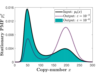
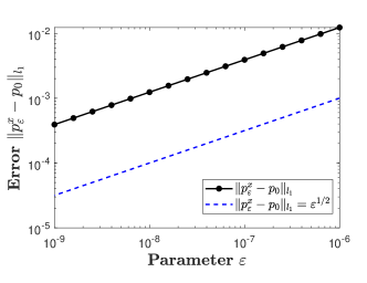
                (a)                                                        (b)

 

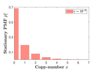
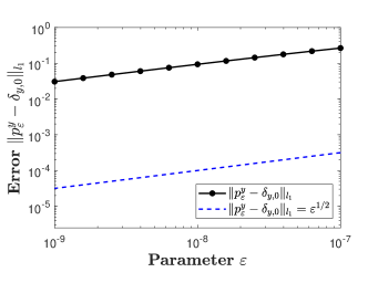
                (c)                                                        (d)

Figure 1: Panel (a) displays the stationary PMF of the input network (28) as a black curve, and the $x$-marginal PMF for the output network  (29), under (30), for different values of the asymptotic parameter $\varepsilon$. Panel (b) displays as black dots, interpolated with the solid lines, a log-log plot of the $l^{1}$-distance between the PMFs for networks (28) and (29) as a function of $\varepsilon$. Analogous plots are shown in panels (c) and (d) for the $y$-marginal PMF for (29). The parameters are fixed to $(k_{1},k_{2},k_{3},k_{4})=(1125,37.5,0.36,10^{-3})$, and $(\tilde{\nu},\bar{\gamma})=(0,1)$.

Let us first satisfy kinetic condition (16) by setting

$$s=1/2,\;\;\bar{\kappa}_{1}=\bar{\kappa}_{2}=k_{4}^{1/2}.$$ (30)

In Figure 1(a), we display the stationary $x$-marginal PMF of the output network (29) under (30), denoted by $p_{\varepsilon}^{x}=p_{\varepsilon}^{x}(x)$, for different values of the parameter $\varepsilon$. In particular, when $\varepsilon=10^{-2}$, the PMF is shown as a dashed purple curve; while bi-modal, this intermediate PMF is inaccurately distributed. On the other hand, when $\varepsilon=10^{-6}$, the PMF $p_{\varepsilon}^{x}$ is shown as a blue histogram, and is in an excellent match with target PMF $p_{0}$. In Figure 1(b), we show a log-log plot of a numerically approximated error $\|p_{\varepsilon}^{x}-p_{0}\|_{l_{1}}$ as a function of $\varepsilon$. Also shown, as a dashed blue line, is the reference curve $\|p_{\varepsilon}^{x}-p_{0}\|_{1}=\varepsilon^{1/2}$; one can notice an excellent match in the slopes of the two curves, in accordance with the finite-time result from Proposition 2.1. In Figure 2(c), we display the $y$-marginal PMF for network (29) when $\varepsilon=10^{-6}$, which is shown in Figure 2(d) to converge, at $\varepsilon^{1/2}$-rate, to the Kronecker-delta distribution centered at zero.

Proposition 2.1 provides information about the error $\|p_{\varepsilon}^{x}-p_{0}\|_{l_{1}}$ in the limit $\varepsilon\to 0$. Let us now discuss how one may decrease the error for a fixed $\varepsilon$ by choosing an appropriate scaling factor $s$. To this end, note that network (2) consists of an ordered chain of reactions: in order for $\mathcal{R}_{2}$ to fire, and mimic (1), one requires that $\mathcal{R}_{1}$ fires first. The reactant of $\mathcal{R}_{1}$, forming the start of the chain, is given by $2X$, and the propensity function is given by $\alpha_{1}(x)=\kappa_{1}x(x-1)$. On the other hand, $\mathcal{R}_{2}$ involves as a reactant the short-lived lower-copy-number species $Y$, with the propensity function $\alpha_{2}(x,y_{1})=\kappa_{2}xy$. Since $Y(t)$ spends most of the time at $y=0$ for smaller $\varepsilon$, it follows that the underlying joint-PMF is concentrated in the neighborhood of the $x$-axis, and $\alpha_{2}(x,y)/\kappa_{2}<\alpha_{1}(x)/\kappa_{1}$. This observation suggests that, for a fixed $\varepsilon$, there is an optimal ratio $\kappa_{1}/\kappa_{2}$, sufficiently small to speed up reaction $\mathcal{R}_{2}$, and sufficiently large to ensure that reaction $\mathcal{R}_{1}$ is triggered often enough. To this end, let us now satisfy (16) by setting

$$s=1/3,\;\;\bar{\kappa}_{1}=\bar{\kappa}_{2}=k_{4}^{1/2}.$$ (31)

In Figure 2(a), we display the stationary $x$-marginal PMF of the output network (29) under (31) when $\varepsilon=10^{-2}$. Comparing Figures 1(a) and 2(a), one can notice that, when $\varepsilon=10^{-2}$, scaling (31) leads to a significantly better approximation than (30). However, comparing Figures 1(b) and 2(b), one can notice that the convergence under the scaling (30) is faster than under (31), with the latter occurring at a rate $\varepsilon^{1/3}$. In Figure 2(c), we display the $l_{1}$-distance between the input and output PMFs as a function of the scaling factor $s$, for fixed $\bar{\kappa}_{1},\bar{\kappa}_{2}$, and for three different values of the parameter $\varepsilon$. One can notice that the error is minimized approximated at $s=3/10$ when $\varepsilon=10^{-2}$, and that, for larger values of $\varepsilon$, an overall better performance is achieved by taking $s<1/2$. Figure 2(c) also suggests that the error does not converge to zero at the degenerate points $s=0$ and $s=1$.

 

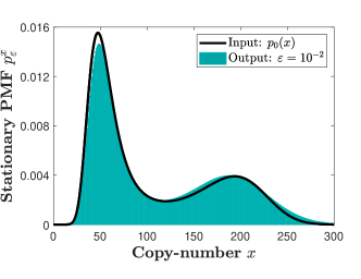
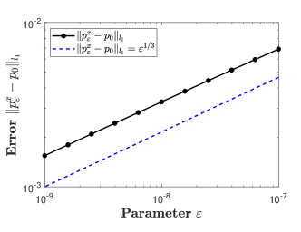
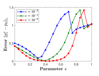
(a)                                                   (b)                                                   (c)

Figure 2: Panel (a) displays the stationary PMF of the input network (28) as a black curve, and the $x$-marginal PMF for the output network  (29), under (31) with $\varepsilon=10^{-2}$, as a blue histogram. Panel (b) displays a log-log plot of the $l^{1}$-distance between the PMFs for networks (28) and (29) as a function of $\varepsilon$. Panel (c) displays the error as a function of the scaling factor $s$, with fixed $\bar{\kappa}_{1},\bar{\kappa}_{2}$ and different values of $\varepsilon$. The parameters are fixed as in Figure 1.

4 General case: Multi-species higher-order reactions

Let us consider an arbitrary $n$th-order reaction, under mass-action kinetics, with $n\geq 3$, involving $N$ biochemical species $\mathcal{X}=\{X_{1},X_{2},\ldots,X_{N}\}$ and $m$ distinct reactants $\{X_{1},X_{2},\ldots,X_{m}\}\subseteq\mathcal{X}$, given by

$$\mathcal{R}_{0}(\mathcal{X}):\;\;\sum_{i=1}^{m}\nu_{i}X_{i} \xrightarrow[]{k}\sum_{i=1}^{N}\bar{\nu}_{i}X_{i},\hskip 8.5359pt\textrm{where }\{\nu_{i}\in\mathbb{Z}_{>}\}_{i=1}^{m}\textrm{ and }\sum_{i=1}^{m}\nu_{i}=n\geq 3.$$ (32)

For convenience, we assume that the reactant species are ordered according to nondecreasing stoichiometric coefficients, $\nu_{i}\leq\nu_{j}$ if $i<j$, for all $i,j\in\{1,2,\ldots,m\}$. Let us also consider the second-order mass-action reaction network $\mathcal{R}_{\varepsilon}$, given by

$$\mathcal{R}_{\varepsilon}(\mathcal{X},\mathcal{Y}) =\begin{cases}\mathcal{R}_{1}^{\varepsilon}(X_{1},X_{1})\,\bigcup_{i=2}^{\nu_{1}-2}\mathcal{R}_{i}^{\varepsilon}(X_{1})\,\bigcup\,\mathcal{R}_{n-1}(X_{1}),&\text{if }m=1,\\ \mathcal{R}_{1}^{\varepsilon}(X_{1},X_{2})\,\bigcup_{i=2}^{\nu_{1}}\mathcal{R}_{i}^{\varepsilon}(X_{1})\,\bigcup_{l=2}^{m-1}\bigcup_{i=\delta_{l,2}+\sum_{j=1}^{l-1}\nu_{j}}^{-1+\sum_{j=1}^{l}\nu_{j}}\mathcal{R}_{i}^{\varepsilon}(X_{l})\\ \,\bigcup_{i=\delta_{m,2}+\sum_{j=1}^{m-1}\nu_{j}}^{n-2}\mathcal{R}_{i}^{\varepsilon}(X_{m})\,\bigcup\,\mathcal{R}_{n-1}(X_{m}),&\text{if }m\geq 2,\end{cases}$$ (33)

with the convention that $\bigcup_{l=a}^{b}\mathcal{R}(l)=\emptyset$ if $a<b$, where $\emptyset$ is the empty set, and with the sub-networks

$$\mathcal{R}_{1}^{\varepsilon}(X_{i},X_{j}):\;\;X_{i}+X_{j} \xrightleftharpoons[1/\varepsilon]{\kappa_{1}}Y_{1},$$

$$\mathcal{R}_{i}^{\varepsilon}(X_{j}):\;\;X_{j}+Y_{i-1} \xrightleftharpoons[1/\varepsilon]{\kappa_{i}}Y_{i},\hskip 8.5359pt\textrm{for all }i\in\{2,3,\ldots,n-2\},$$

$$\mathcal{R}_{n-1}(X_{j}):\;\;X_{j}+Y_{n-2} \xrightarrow[]{\kappa_{n-1}}\sum_{i=1}^{m}\tilde{\nu}_{i}X_{i}+\sum_{i=m+1}^{N}\bar{\nu}_{i}X_{i}+\sum_{i=1}^{n-2}\bar{\gamma}_{i}Y_{i}.$$ (34)

Network $\mathcal{R}_{\varepsilon}=\mathcal{R}_{\varepsilon}(\mathcal{X},\mathcal{Y})$, given by (33)–(34), contains $(n-2)$ auxiliary species $\mathcal{Y}=\{Y_{1},Y_{2},\ldots,Y_{n-2}\}$, and consists of $(2n-3)$ reactions, $(n-2)$ of which are first-order, and $(n-1)$ of second-order. Reaction network (2) from Section 2 is a special case of (33)–(34) with $n=3$ and $m=1$.

4.1 Kinetic and stoichiometric conditions

In Appendix B, we generalize the formal perturbation analysis performed for network (2) in Section 2.1 to the network (33)–(34), and show that the CMEs for input network (32) and output network (33)–(34) match under suitable generalizations of the kinetic and stoichiometric conditions (16)–(17). In particular, the generalized kinetic condition is given by

$$\varepsilon^{n-2}\prod_{i=1}^{n-1}\kappa_{i} =k,\;\;\;\textrm{where }\kappa_{1},\kappa_{2},\ldots,\kappa_{n-1}=o(\varepsilon^{-1})\;\;\text{as }\varepsilon\to 0.$$ (35)

Requirement (35) states that the product of the rate coefficients of the slower reactions from (34), $\prod_{i=1}^{n-1}\kappa_{i}$, divided by the product of the rate coefficient of the faster reaction, $1/\varepsilon^{n-2}$, must be equal to the rate coefficient of (32), $k$. On the other hand, when the reaction $\mathcal{R}_{n-1}(X_{m})$ from (34) does not contain the auxiliary species $\{Y_{1},Y_{2},\ldots,Y_{n-3}\}$, then the stoichiometric conditions are given by

$$\tilde{\nu}_{i} =\bar{\nu}_{i}-(\nu_{i}-\delta_{i,m})\bar{\gamma}_{n-2},\;\;\textrm{for all }i\in\{1,2,\ldots,m\},\;\;\;\textrm{if }(\bar{\gamma}_{1},\bar{\gamma}_{2},\ldots,\bar{\gamma}_{n-3})=(0,0,\ldots,0).$$ (36)

Stoichiometric conditions valid when $(\bar{\gamma}_{1},\bar{\gamma}_{2},\ldots,\bar{\gamma}_{n-3})\neq\mathbf{0}$ take a more complicated form, and can be obtained algebraically as explained in Appendix B. For any particular reaction network, stoichiometric conditions are readily obtainable, as we now outline via an example.

Example 4.1.

Consider the fourth-order input reaction

$$\mathcal{R}_{0}(X_{1},X_{2}):\;\;2X_{1}+2X_{2} \xrightarrow[]{k}4X_{1}+4X_{2},$$ (37)

with the reactant and product stoichiometric vectors $(\nu_{1},\nu_{2})=(2,2)$ and $(\bar{\nu}_{1},\bar{\nu}_{2})=(4,4)$, respectively, and the reaction vector $(\Delta x_{1},\Delta x_{2})=(4,4)-(2,2)=(2,2)$. Output network (33)–(34) takes the form $\mathcal{R}_{\varepsilon}=\mathcal{R}_{1}^{\varepsilon}(X_{1},X_{2})\cup\mathcal{R}_{2}^{\varepsilon}(X_{1})\cup\mathcal{R}_{3}(X_{2})$, with

$$\mathcal{R}_{1}^{\varepsilon}(X_{1},X_{2}):\;\;X_{1}+X_{2} \xrightleftharpoons[1/\varepsilon]{\kappa_{1}}Y_{1},$$

$$\mathcal{R}_{2}^{\varepsilon}(X_{2}):\;\;X_{1}+Y_{1} \xrightleftharpoons[1/\varepsilon]{\kappa_{2}}Y_{2},$$

$$\mathcal{R}_{3}(X_{2}):\;\;X_{2}+Y_{2} \xrightarrow[]{\kappa_{3}}\tilde{\nu}_{1}X_{1}+\tilde{\nu}_{2}X_{2}+\bar{\gamma}_{1}Y_{1}+\bar{\gamma}_{2}Y_{2}.$$ (38)

General stoichiometric conditions required for matching networks (37)–(38) are obtained from the conservation laws that are locally valid for the fastest two reactions from (38):

$$\bar{x}_{1} =x_{1}+y_{1}+2y_{2},$$

$$\bar{x}_{2} =x_{2}+y_{1}+y_{2}.$$ (39)

Applying the difference operator $\Delta$ on (39), and setting $(\Delta\bar{x}_{1},\Delta\bar{x}_{2})=(\Delta x_{1},\Delta x_{2})$, one obtains the stoichiometric conditions

$$\tilde{\nu}_{1} =4-(\bar{\gamma}_{1}+2\bar{\gamma}_{2}),$$

$$\tilde{\nu}_{2} =4-(\bar{\gamma}_{1}+\bar{\gamma}_{2}).$$ (40)

Conditions (40) can also be applied graphically using the formal equalities $Y_{1}\doteq(X_{1}+X_{2})$ and $Y_{2}\doteq(X_{1}+Y_{1})=(2X_{1}+X_{2})$. In particular, taking $(\bar{\gamma}_{1},\bar{\gamma}_{2})=(0,0)$, equation (36) (or (40)) implies that $(\tilde{\nu}_{1},\tilde{\nu}_{2})=(\bar{\nu}_{1},\bar{\nu}_{2})$, i.e. reactions $\mathcal{R}_{3}(X_{2})$ from (38) and (37) have identical products:

$$\mathcal{R}_{3}(X_{2}):\;\;X_{2}+Y_{2} \xrightarrow[]{\kappa_{3}}4X_{1}+4X_{2},\hskip 8.5359pt\textrm{if }(\bar{\gamma}_{1},\bar{\gamma}_{2})=(0,0).$$ (41)

One can add $\varnothing\doteq(Y_{1}-X_{1}-X_{2})$ and $\varnothing\doteq(Y_{2}-2X_{1}-X_{2})$ to the products in (41) as many times as desired, as long as the resulting complex contains nonnegative stoichiometric coefficients. For example, by adding the complex $\varnothing\doteq(Y_{2}-2X_{1}-X_{2})$ once to (41), one obtains

$$\mathcal{R}_{3}(X_{2}):\;\;X_{2}+Y_{2} \xrightarrow[]{\kappa_{3}}2X_{1}+3X_{2}+Y_{2},\hskip 8.5359pt\textrm{if }(\bar{\gamma}_{1},\bar{\gamma}_{2})=(0,1).$$ (42)

Adding the complex $\varnothing\doteq(Y_{1}-X_{1}-X_{2})$ four times to (41) leads to

$$\mathcal{R}_{3}(X_{2}):\;\;X_{2}+Y_{2} \xrightarrow[]{\kappa_{3}}4Y_{1},\hskip 8.5359pt\textrm{if }(\bar{\gamma}_{1},\bar{\gamma}_{2})=(4,0),$$ (43)

while adding $\varnothing\doteq(Y_{1}-X_{1}-X_{2})$ twice, and $\varnothing\doteq(Y_{2}-2X_{1}-X_{2})$ once, results in

$$\mathcal{R}_{3}(X_{2}):\;\;X_{2}+Y_{2} \xrightarrow[]{\kappa_{3}}X_{2}+2Y_{1}+Y_{2},\hskip 8.5359pt\textrm{if }(\bar{\gamma}_{1},\bar{\gamma}_{2})=(2,1).$$ (44)

On the other hand, adding $\varnothing\doteq(Y_{2}-2X_{1}-X_{2})$ three times to the products in (41) leads to

$$\mathcal{R}_{3}(X_{2}):\;\;X_{2}+Y_{2} \xrightarrow[]{\kappa_{3}}-2X_{1}+X_{2}+3Y_{2},\hskip 8.5359pt\textrm{if }(\bar{\gamma}_{1},\bar{\gamma}_{2})=(0,3),$$ (45)

which is not a chemical reaction, as the product complex is not nonnegative. ∎

Remark. The approach taken in Example 4.1 applies generally: one can extract the formal equalities, such as $\varnothing\doteq(Y_{1}-X_{1}-X_{2})$ and $\varnothing\doteq(Y_{2}-2X_{1}-X_{2})$, directly from $\mathcal{R}_{\varepsilon}$. Writing the final reaction from $\mathcal{R}_{\varepsilon}$ with the same product complex as in the original reaction $\mathcal{R}_{0}$, one can then add the formal equalities as many times as desired to the products of $\mathcal{R}_{0}$, provided the resulting complex remains nonnegative.

4.2 Convergence

We now generalize Proposition 2.1, by establishing convergence when the slower rate coefficients from (33)–(34) are all scaled identically:

$$\kappa_{i} =\varepsilon^{-(n-2)/(n-1)}\bar{\kappa}_{i},\;\;\;\;\textrm{for all }i\in\{1,2,\ldots,n-1\},$$ (46)

where $\{\bar{\kappa}_{i}\}_{i=1}^{n-1}$ are $\varepsilon$-independent parameters. To this end, consider the PMF

$$p_{0}(\mathbf{\bar{x}},\mathbf{y},t) =p_{0}(\mathbf{\bar{x}},t)\prod_{i=1}^{n-2}\delta_{y_{i},0},$$ (47)

where $\mathbf{\bar{x}}\in\mathbb{Z}_{\geq}^{N}$ is given by (66)–(67) in Appendix B, $\mathbf{y}\in\mathbb{Z}_{\geq}^{n-2}$, and the PMF $p_{0}(\mathbf{\bar{x}},t)$ satisfies

$$\frac{\mathrm{d}}{\mathrm{d}t}p_{0}(\mathbf{\bar{x}},t) =\left(E_{\mathbf{\bar{x}}}^{-\Delta\bar{\mathbf{x}}}-1\right)\left(\prod_{j=1}^{n-1}\bar{\kappa}_{j}\right)\prod_{l=1}^{m}\bar{x}_{l}^{\underline{\nu_{l}}}p_{0}(\mathbf{\bar{x}},t),$$ (48)

where $\Delta\mathbf{\bar{x}}$ is obtained by applying the difference operator $\Delta$ on (66)–(67). Note that, under the kinetic and stoichiometric conditions from Section 4.1, CME (48) is identical to the CME of the original network (32).

Theorem 4.1.

Consider network $\mathcal{R}_{\varepsilon}$, given by (33)–(34), with the rate coefficients $\{\kappa_{i}\}_{i=1}^{n-1}$ given by (46), and with the PMF $p_{\varepsilon}(\mathbf{\bar{x}},\mathbf{y},t)$ satisfying (69). Let the PMF $p_{0}(\mathbf{\bar{x}},\mathbf{y},t)$ satisfy (47)–(48), and assume that $p_{\varepsilon}(\mathbf{\bar{x}},\mathbf{y},0)=p_{0}(\mathbf{\bar{x}},\mathbf{y},0)$. Then, for every $\mathbb{S}\subset\mathbb{Z}_{\geq}^{N+(n-2)}$ and every $T>0$ there exists an $\varepsilon$-independent constant $c>0$ such that

$$\left\|p_{\varepsilon}(\mathbf{\bar{x}},\mathbf{y},t)-p_{0}(\mathbf{\bar{x}},\mathbf{y},t)\right\|_{l_{1}(\mathbb{S})} \leq c\,\varepsilon^{1/(n-1)},\;\;\textrm{as }\varepsilon\to 0,\;\;\textrm{for all }t\in[0,T].$$ (49)

Proof.

See Appendix C. ∎

Remark. The error estimate (49) is independent of how the stoichiometric coefficients $\{\tilde{\nu}_{i}\}_{i=1}^{m}$, $\{\bar{\nu}_{i}\}_{i=m+1}^{N}$ and $\{\bar{\gamma}_{i}\}_{i=1}^{n-2}$ from (34) are chosen.

To formulate Theorem 4.1, we have assumed a fixed ordering of the reactants and reactions in (33)–(34). One can readily prove analogous results for other suitable orderings.

Example 4.2.

Consider the third-order input reaction

$$\mathcal{R}_{0}(X_{1},X_{2}):\;\;X_{1}+2X_{2} \xrightarrow[]{k}\varnothing.$$ (50)

Output network (33)–(34) is given by $\mathcal{R}_{\varepsilon}=\mathcal{R}_{1}^{\varepsilon}(X_{1},X_{2})\cup\mathcal{R}_{2}(X_{2})$, where

$$\mathcal{R}_{1}^{\varepsilon}(X_{1},X_{2}):\;\;X_{1}+X_{2}\xrightleftharpoons[1/\varepsilon]{\kappa_{1}}Y_{1},$$

$$\mathcal{R}_{2}(X_{2}):\;\;X_{2}+Y_{1}\xrightarrow[]{\kappa_{2}}\varnothing;$$ (51)

in particular, the forward reaction from $\mathcal{R}_{1}^{\varepsilon}$ is a second-order hetero-reaction, involving two distinct reactants $X_{1}$ and $X_{2}$. One can readily show that the results presented in this section also hold for the output network $\mathcal{R}_{1}^{\varepsilon}(X_{2},X_{2})\cup\mathcal{R}_{2}(X_{1})$, given by

$$\mathcal{R}_{1}^{\varepsilon}(X_{2},X_{2}):\;\;2X_{2}\xrightleftharpoons[1/\varepsilon]{\kappa_{1}}Y_{1},$$

$$\mathcal{R}_{2}(X_{1}):\;\;X_{1}+Y_{1}\xrightarrow[]{\kappa_{2}}\varnothing,$$ (52)

for which the forward reaction from $\mathcal{R}_{1}^{\varepsilon}$ is a second-order homo-reaction, involving $X_{2}$. Another valid output network is $\mathcal{R}_{1}^{\varepsilon}(X_{1},\varnothing)\cup\mathcal{R}_{2}^{\varepsilon}(X_{2})\cup\mathcal{R}_{3}(X_{2})$, given by

$$\mathcal{R}_{1}^{\varepsilon}(X_{1},\varnothing):\;\;X_{1}\xrightleftharpoons[1/\varepsilon]{\kappa_{1}}Y_{1},$$

$$\mathcal{R}_{2}^{\varepsilon}(X_{2}):\;\;X_{2}+Y_{1}\xrightleftharpoons[1/\varepsilon]{\kappa_{2}}Y_{2},$$

$$\mathcal{R}_{3}(X_{1}):\;\;X_{2}+Y_{2}\xrightarrow[]{\kappa_{3}}\varnothing,$$ (53)

for which the forward reaction from $\mathcal{R}_{1}^{\varepsilon}$ is of first-order. ∎

5 Examples: Noise-induced phenomena

In this section, we apply the results from Section 4 to two test networks arising from theoretical synthetic biology and displaying noise-induced dynamical phenomena. In particular, the first network, given by (54), plays an important role in the stochastic morpher controller [8] that can globally morph PMF of a given reaction network into any desired form. The second network, given by (58), is a part of the noise-control algorithm [10] that can redesign a given reaction network to locally reshape the underlying PMF in a mean-preserving manner.

5.1 Biochemical Kronecker-delta distribution

Let us consider the fourth-order mass-action input reaction network

$$\mathcal{R}_{0}(X):\;\;\varnothing \xrightarrow[]{k_{1}}X,$$

$$4X \xrightarrow[]{k_{2}}3X.$$ (54)

Long-time PMF of (54), under a particular choice of the rate coefficients $k_{1}<k_{2}$, is shown in Figure 3(a) as black dots interpolated with solid lines. The PMF is approximately the Kronecker-delta distribution centered $x=3$. In particular, when there are less than four molecules of $X$ present, $x<4$, only the first reaction from (54) fires and $X$ experiences a constant positive drift until four molecules are present. When $x\geq 4$, both reactions from (54) fire, with the second one, having a larger propensity function, overpowering the first one and generating a net-negative drift. The combined effect of the two reactions forces $X$ to spend most of the time at the state $x=3$.

The fourth-order input network (54) can be approximated with a second-order output one using the results from Section 4. In particular, applying the algorithm (33)–(34), a suitable output network is given by $\mathcal{R}\cup\mathcal{R}_{1}^{\varepsilon}\cup\mathcal{R}_{2}^{\varepsilon}\cup\mathcal{R}_{4}$, where

$$\;\,\mathcal{R}(X):\; \varnothing \xrightarrow[]{k_{1}}X,$$

$$\mathcal{R}_{1}^{\varepsilon}(X):\; 2X \xrightleftharpoons[1/\varepsilon]{\kappa_{1}}Y_{1},$$

$$\mathcal{R}_{2}^{\varepsilon}(X):\; X+Y_{1} \xrightleftharpoons[1/\varepsilon]{\kappa_{2}}Y_{2},$$

$$\mathcal{R}_{4}(X):\; X+Y_{2} \xrightarrow[]{\kappa_{3}}\tilde{\nu}X+\bar{\gamma}_{1}Y_{1}+\bar{\gamma}_{2}Y_{2}.$$ (55)

Let us fix $(\bar{\gamma}_{1},\bar{\gamma}_{2})=(0,1)$, so that $\tilde{\nu}=0$ by the stoichiometric condition (36). On the other hand, the kinetic condition (35) for (55) takes the form

$$\varepsilon^{2}\kappa_{1}\kappa_{2}\kappa_{3} =k_{2},\;\;\;\textrm{where }\kappa_{1},\kappa_{2},\kappa_{3},\kappa_{4}=o(\varepsilon^{-1})\;\;\text{as }\varepsilon\to 0,$$ (56)

which is satisfied with e.g.

$$\kappa_{1} =k_{2}\varepsilon^{-2/3},\;\;\kappa_{2}=\varepsilon^{-2/3},\;\;\kappa_{3}=\varepsilon^{-2/3}.$$ (57)

In Figure 3(a), we display the long-time $x$-marginal PMF of network (55) under the rate coefficients (57) with $\varepsilon=10^{-3}$, which is in an excellent agreement with the input PMF. In Figure 3(b), we show that the output PMF converges to the input one at a rate $\varepsilon^{1/3}$, consistent with Theorem 4.1.

 

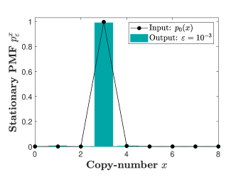
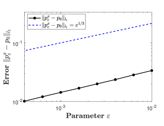
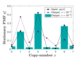
(a)                                                  (b)                                                   (c)

Figure 3: Panel (a) displays the long-time PMF of the input network (54) with $(k_{1},k_{2})=(10^{-3},10^{-2})$ as black dots interpolated with solid lines; the long-time $x$-marginal PMF of the output network (55), with $(\tilde{\nu},\bar{\gamma}_{1},\bar{\gamma}_{2})=(0,0,1)$, under rate coefficients (57), is shown as a blue histogram when $\varepsilon=10^{-2}$. Panel (b) displays a log-log plot of the $l^{1}$-distance between the long-time PMFs for networks (54) and (55). Panel (c) displays the long-time PMF of the input network (58) with $(k_{1},k_{2},k_{2,5},\tilde{k}_{4,2})=(1,1,1,1)$, and the $x$-marginal PMF of the output network (59), under rate coefficients (61) with $\beta=1/12$, for two different values of $\varepsilon$. The conservation constant for (58) is fixed to $c=7$, and (59) is initialized with zero copy-numbers of the species $\{Y_{i}\}_{i=1}^{5}$ and $\tilde{Y}_{4}$.

5.2 Noise-induced tri-modality

In Section 4, we have provided an algorithm for approximating a single higher-order input reaction (32) with a second-order network of the form (33)–(34). A generalization to the case when the input network contains multiple higher-order reactions is straightforward: each of the desired higher-order reaction can be separately approximated with a suitable network of the form (33)–(34), while the other input reactions, which one does not wish to approximate, are copied directly to the output network without any modifications. However, such an output network may be biochemically expensive to engineer, as it may contain a larger number of the auxiliary reactions and species $\mathcal{Y}$. This undesirable feature can be reduced when some of the higher-order input reactions involve common reactant sub-complexes; then, some of the intermediate species $\mathcal{Y}$ may be re-used to simultaneously approximate multiple input reactions. Put it another way, reactions with common sub-complexes can be approximated by multiple chains of reactions of the form (34), which all branch out from a suitable common sub-chain, provided the underlying kinetic conditions can be satisfied. These statements readily follow from the perturbation analysis performed in this paper. To illustrate these ideas, consider the seventh-order mass-action input network $\mathcal{R}_{0}=\mathcal{R}\cup\mathcal{R}_{2,5}\cup\mathcal{R}_{4,2}$, given by

$$\mathcal{R}(X_{1},X_{2}):\; X_{2} \xrightleftharpoons[k_{2}]{k_{1}}X_{1},$$

$$\mathcal{R}_{2,5}(X_{1},X_{2}):\; 2X_{1}+5X_{2} \xrightarrow[]{k_{2,5}}3X_{1}+4X_{2},$$

$$2X_{1}+5X_{2} \xrightarrow[]{k_{2,5}}X_{1}+6X_{2},$$

$$\mathcal{\tilde{R}}_{4,2}(X_{1},X_{2}):\; 4X_{1}+2X_{2} \xrightarrow[]{\tilde{k}_{4,2}}5X_{1}+X_{2},$$

$$4X_{1}+2X_{2} \xrightarrow[]{\tilde{k}_{4,2}}3X_{1}+3X_{2}.$$ (58)

Species $X_{1}$ and $X_{2}$ from (58) are conserved, $x_{1}+x_{2}=c$; in what follows, we fix the conservation constant to $c=7$. Reaction network (58) has been obtained by applying the noise-control algorithm [10] on network $\mathcal{R}(X_{1},X_{2})$; in particular, sub-networks $\mathcal{R}_{2,5}$ and $\mathcal{\tilde{R}}_{4,2}$, called zero-drift networks, introduce a state-dependent noise, and decrease the PMF of network $\mathcal{R}(X_{1},X_{2})$, at $x_{1}=2$ and $x_{1}\in\{4,5\}$, respectively, while preserving the underlying mean. In Figure 3(c), we display the long-time PMF of (58) as black dots interpolated with solid lines. One can notice that the network displays noise-induced tri-modality, with the modes $x_{1}\in\{1,3,6\}$.

Using (33)–(34) to independently reduce order of the network $\mathcal{R}_{2,5}\cup\mathcal{\tilde{R}}_{4,2}$ from seven to two requires $18$ auxiliary species and $40$ reactions in total, i.e. $10$ independent auxiliary species for the network $\mathcal{R}_{2,5}$ ($5$ species for each of the underlying reactions) and, similarly, $8$ species for $\mathcal{\tilde{R}}_{4,2}$. However, since each of the two reactions from $\mathcal{R}_{2,5}$ involves the same reactants, one can reduce their order simultaneously by using $5$ auxiliary species; similarly, $4$ auxiliary species suffice to reduce order of the network $\mathcal{\tilde{R}}_{4,2}$. Furthermore, all of the reactions from $\mathcal{R}_{2,5}\cup\mathcal{\tilde{R}}_{4,2}$ involve a common reactant sub-complex $(2X_{1}+2X_{2})$, so that, instead of using $9$ auxiliary species for $\mathcal{R}_{2,5}\cup\mathcal{\tilde{R}}_{4,2}$, one can use only $6$; a resulting output network is given by

$$\mathcal{R}(X_{1},X_{2}):\; X_{2} \xrightleftharpoons[k_{2}]{k_{1}}X_{1},$$

$$\mathcal{R}_{1}^{\varepsilon}(X_{1},X_{1}):\; 2X_{1} \xrightleftharpoons[1/\varepsilon]{\kappa_{1}}Y_{1},$$

$$\mathcal{R}_{2}^{\varepsilon}(X_{2}):\; X_{2}+Y_{1} \xrightleftharpoons[1/\varepsilon]{\kappa_{2}}Y_{2},$$

$$\mathcal{R}_{3}^{\varepsilon}(X_{2}):\; X_{2}+Y_{2} \xrightleftharpoons[1/\varepsilon]{\kappa_{3}}Y_{3},$$

$$\mathcal{R}_{4}^{\varepsilon}(X_{2}):\; X_{2}+Y_{3} \xrightleftharpoons[1/\varepsilon]{\kappa_{4}}Y_{4},$$

$$\mathcal{R}_{5}^{\varepsilon}(X_{2}):\; X_{2}+Y_{4} \xrightleftharpoons[1/\varepsilon]{\kappa_{5}}Y_{5},$$

$$\mathcal{R}_{6}(X_{1}):\; X_{2}+Y_{5} \xrightarrow[]{\kappa_{6}}3X_{1}+4X_{2},$$

$$X_{2}+Y_{5} \xrightarrow[]{\kappa_{6}}X_{1}+6X_{2},$$

$$\tilde{\mathcal{R}}_{4}^{\varepsilon}(X_{1}):\; X_{1}+Y_{3} \xrightleftharpoons[1/\varepsilon]{\tilde{\kappa}_{4}}\tilde{Y}_{4},$$

$$\tilde{\mathcal{R}}_{5}(X_{1}):\; X_{1}+\tilde{Y}_{4} \xrightarrow[]{\tilde{\kappa}_{5}}5X_{1}+X_{2},$$

$$X_{1}+\tilde{Y}_{4} \xrightarrow[]{\tilde{\kappa}_{5}}3X_{1}+3X_{2}.$$ (59)

The sub-network $\mathcal{R}_{2,5}$ is approximated by $\bigcup_{i=1}^{5}\mathcal{R}_{i}^{\varepsilon}\cup\mathcal{R}_{6}$, while $\mathcal{\tilde{R}}_{4,2}$ by $\bigcup_{i=1}^{3}\mathcal{R}_{i}^{\varepsilon}\cup\tilde{\mathcal{R}}_{4}^{\varepsilon}\cup\tilde{\mathcal{R}}_{5}$. Instead of using $18$ auxiliary species and $40$ reactions to independently approximate all the higher-order reactions from (58) by second-orders ones, we have achieved the same goal in (59) with $6$ auxiliary species and $16$ reactions.

Network (59) satisfies the stoichiometric conditions (36), since $\mathcal{R}_{6}$ and $\tilde{\mathcal{R}}_{5}$ do not contain any auxiliary species $\mathcal{Y}=\{Y_{1},Y_{2},Y_{3},Y_{4},Y_{5},\tilde{Y}_{4}\}$ as products. One can reduce the product stoichiometric coefficients of $X_{1}$ and $X_{2}$ in $\mathcal{R}_{6}$ and $\tilde{\mathcal{R}}_{5}$ by introducing suitable species $\mathcal{Y}$ as products (see also Example 4.1); for simplicity, we consider the form (59) in this paper. On the other hand, kinetic conditions (35) take the form

$$\varepsilon^{5}\kappa_{1}\kappa_{2}\kappa_{3}\kappa_{4}\kappa_{5}\kappa_{6} =k_{2,5},\;\;\;\textrm{where }\kappa_{1},\kappa_{2},\ldots,\kappa_{6}=o(\varepsilon^{-1})\;\;\text{as }\varepsilon\to 0,$$

$$\varepsilon^{4}\kappa_{1}\kappa_{2}\kappa_{3}\tilde{\kappa}_{4}\tilde{\kappa}_{5} =\tilde{k}_{4,2},\;\;\;\textrm{where }\tilde{\kappa}_{4},\tilde{\kappa}_{5}=o(\varepsilon^{-1})\;\;\text{as }\varepsilon\to 0.$$ (60)

Guided by the discussion in Section 3 (see also Figure 2(c)), to achieve a higher accuracy for larger values of $\varepsilon$, we satisfy the kinetic conditions with

$$\kappa_{1} =\left(\varepsilon^{-\frac{5}{6}}(k_{2,5})^{\frac{1}{6}}\right)\varepsilon^{5\beta},$$

$$\kappa_{i} =\left(\varepsilon^{-\frac{5}{6}}(k_{2,5})^{\frac{1}{6}}\right)\varepsilon^{-\beta},\;\;0\leq\beta<1/6,\;\;\textrm{for all }i\in\{2,3,4,5,6\},$$

$$\tilde{\kappa}_{i} =\varepsilon^{-2}(\kappa_{1}\kappa_{2}\kappa_{3})^{-\frac{1}{2}}(\tilde{k}_{4,2})^{\frac{1}{2}},\;\;\textrm{for all }i\in\{4,5\}.$$ (61)

In Figure 3(c), we display the long-time $x$-marginal PMF of (59) with rate coefficients (61), with the auxiliary parameter $\beta=1/12$, for $\varepsilon=10^{-3}$ and $\varepsilon=10^{-6}$, the latter of which is in a good agreement with the long-time PMF of the input network (58).

6 Discussion

In this paper, we have shown that, by introducing suitable time-scale separations and dimension expansion (introduction of auxiliary reactions and species), any higher-order input reaction can be mapped to a suitable second-order output network, with the underlying stochastic dynamics being preserved. In particular, the time-dependent probability distributions of the input and output networks are arbitrarily close over bounded time-intervals in an appropriate asymptotic limit of some of the underlying rate coefficients. The results presented in this paper generalize the deterministic order-reduction algorithm for third- and fourth-order reactions from [21, 22, 23] to the stochastic regime and to reactions with arbitrary order.

In Section 2, we have shown that an arbitrary one-species reaction of order $n=3$, given by (1), can be approximated by a family of second-order networks (2), provided the kinetic and stoichiometric conditions (16) and (17), respectively, are satisfied. Convergence for a family of the output networks has been proved in Proposition 2.1. In Section 3, we have verified the results from Section 2 on the Schlögl network (28), and we have discussed different ways to satisfy the kinetic condition (16). In Appendices B–C, we have generalized the results from Section 2 to arbitrary multi-species reactions of order $n\geq 3$, and have presented these results in Section 4. In particular, we have shown that any reaction of the form (32) can be approximated with a family of second-order networks (33)–(34) that satisfies the generalized kinetic and stoichiometric conditions (35)–(36); convergence for a family of such networks is presented as Theorem 4.1. For an input network of order $n\geq 3$, the order of convergence is shown to be given by $1/(n-1)$, and is independent of the stoichiometry of the output networks. In Section 5, we have applied the results from Section 4 to the fourth- and seventh-order input networks (54) and (58), respectively, arising from theoretical synthetic biology [10, 8], and displaying noise-induced phenomena that are absent at the deterministic level. In this context, we have discussed how multiple higher-order input reactions can be mapped more efficiently into smaller output networks.

The results established in this paper may play an important role in synthetic biology, and particularly in nucleic-acid-based synthetic biology, also known as DNA computing [13]. In this context, it has been proved that, assuming one can experimentally vary reaction rate coefficients over a sufficiently large range, any abstract second-order reaction network, under mass-action kinetics, can be experimentally compiled into a physical second-order network with DNA molecules, with the underlying deterministic dynamics being preserved over bounded time-intervals [6]. This molecular compiler has been proved to also preserve the underlying stochastic dynamics [10]. In this context, results from Section 4, and Theorem 4.1 in particular, imply the following corollary.

Corollary 6.1.

(Universal molecular compiler) Assume that the reaction rate coefficients in the DNA compiler from [6] can be varied over arbitrarily large range. Then, mass-action input reaction networks of any order can be compiled into second-order DNA-based output networks via the compiler from [6], in such a way that the probability distributions for the input and output networks are arbitrarily close over any bounded time-interval.

Appendix A Appendix: Background

Notation. Union and intersection of sets $\mathcal{A}_{1}$ and $\mathcal{A}_{2}$ are denoted by $\mathcal{A}_{1}\cup\mathcal{A}_{2}$ and $\mathcal{A}_{1}\cap\mathcal{A}_{2}$, respectively. The empty set is denoted by $\emptyset$. Set $\mathbb{R}$ is the space of real numbers, $\mathbb{R}_{\geq}$ the space of nonnegative real numbers, and $\mathbb{R}_{>}$ the space of positive real numbers. Similarly, $\mathbb{Z}$ is the space of integer numbers, $\mathbb{Z}_{\geq}$ the space of nonnegative integer numbers, and $\mathbb{Z}_{>}$ the space of positive integer numbers. Euclidean row-vectors are denoted in boldface, $\mathbf{x}=(x_{1},x_{2},\ldots,x_{N})\in\mathbb{R}^{N}=\mathbb{R}^{1\times N}$; the zero vector is given by $\mathbf{0}=(0,0,\ldots,0)\in\mathbb{R}^{N}$. Given two sequences $p,q:\mathbb{Z}_{\geq}^{N}\to\mathbb{R}$, their $l^{2}$ inner-product is given by $\langle p(\mathbf{x}),q(\mathbf{x})\rangle_{\mathbf{x}}=\sum_{\mathbf{x}\in\mathbb{Z}_{\geq}^{N}}p(\mathbf{x})q(\mathbf{x})$; the $l^{1}$-norm of $p(\mathbf{x})$ is given by $\|p(\mathbf{x})\|_{l_{1}}=\sum_{\mathbf{x}\in\mathbb{Z}_{\geq}^{N}}|p(\mathbf{x})|$. Function $\delta_{\cdot,x_{0}}:\mathbb{Z}\to[0,1]$ with parameter $x_{0}\in\mathbb{Z}$, defined by $\delta_{x,x_{0}}=1$ if $x=x_{0}$, and $\delta_{x,x_{0}}=0$ if $x\neq x_{0}$, is called the Kronecker-delta distribution centered at $x_{0}$. Given two functions $f,g:\mathbb{R}_{>}\to\mathbb{R}$, we write $f(\varepsilon)=o(g(\varepsilon))$ as $\varepsilon\to 0$ if $\lim_{\varepsilon\to 0}f(\varepsilon)/g(\varepsilon)=0$; we write $f(\varepsilon)=O(g(\varepsilon))$ as $\varepsilon\to 0$ if $\lim_{\varepsilon\to 0}|f(\varepsilon)|/|g(\varepsilon)|<\infty$.

A.1 Biochemical reaction networks

We consider reaction networks $\mathcal{R}=\mathcal{R}(\mathcal{X})$ firing in well-mixed unit-volume reactors under mass-action kinetics [1], involving $N$ biochemical species $\mathcal{X}=\{X_{1},X_{2},\ldots,X_{N}\}$ interacting via $M$ reactions given by

$$\mathcal{R}(\mathcal{X}):\;\;\sum_{i=1}^{N}\nu_{j,i}X_{i} \xrightarrow[]{k_{j}}\sum_{i=1}^{N}\bar{\nu}_{j,i}X_{i},\,\,\,\,\,\,\,j\in\{1,2,\ldots,M\}.$$ (62)

Here, $k_{j}\in\mathbb{R}_{>}$ is the rate coefficient of the $j$-reaction, and we let $\mathbf{k}\equiv(k_{1},k_{2},\ldots,k_{M})\in\mathbb{R}_{>}^{M}$. Integers $\nu_{j,l},\bar{\nu}_{j,l}\in\mathbb{Z}_{\geq}$ are the reactant and product stoichiometric coefficients of the species $X_{l}$ in the $j$-reaction, respectively, and we let $\boldsymbol{\nu}_{j}\equiv(\nu_{j,1},\nu_{j,2},\ldots,\nu_{j,N})\in\mathbb{Z}_{\geq}^{N}$ and $\bar{\boldsymbol{\nu}}_{j}\equiv(\bar{\nu}_{j,1},\bar{\nu}_{j,2},\ldots,\bar{\nu}_{j,N})\in\mathbb{Z}_{\geq}^{N}$. If $\boldsymbol{\nu}_{j}=\mathbf{0}$ (respectively, $\bar{\boldsymbol{\nu}}_{j}=0$), then the reactant (respectively, product) of the $j$-reaction is the zero species, denoted by $\varnothing$, representing species that are not explicitly modelled. We denote two irreversible reactions $(\sum_{l=1}^{N}\nu_{i,l}X_{l}\xrightarrow[]{k_{i}}\sum_{l=1}^{N}\bar{\nu}_{i,l}X_{l})\in\mathcal{R}$ and $(\sum_{l=1}^{N}\bar{\nu}_{i,l}X_{l}\xrightarrow[]{k_{j}}\sum_{l=1}^{N}\nu_{i,l}X_{l})\in\mathcal{R}$ jointly as the single reversible reaction $(\sum_{l=1}^{N}\nu_{i,l}X_{l}\xrightleftharpoons[k_{j}]{k_{i}}\sum_{l=1}^{N}\bar{\nu}_{i,l}X_{l})\in\mathcal{R}$. The order of j-reaction from network $\mathcal{R}$ is given by $\langle\mathbf{1},\boldsymbol{\nu}_{j}\rangle\in\mathbb{Z}_{\geq}$. The order of reaction network $\mathcal{R}$ is given by the order of its highest-order reaction; $\mathcal{R}$ of order higher than two is said to be a higher-order network.

A.2 Stochastic model of reaction networks

A suitable stochastic model for the time-evolution of discrete species copy-numbers $\mathbf{X}(t)=(X_{1}(t),\ldots,$ $X_{N}(t))\in\mathbb{Z}_{\geq}^{N}$, where $t\in\mathbb{R}_{\geq}$ is the time-variable, is a continuous-time discrete-space Markov chain [28]. The underlying probability mass function (PMF) satisfies a partial difference-differential equation, called the chemical master equation (CME) [33, 34], given by

$$\frac{\partial}{\partial t}p(\mathbf{x},t)=\mathcal{L}p(\mathbf{x},t) =\sum_{j=1}^{M}(E_{\mathbf{x}}^{-\Delta\mathbf{\mathbf{x}}_{j}}-1)\big{(}\alpha_{j}(\mathbf{x})p(\mathbf{x},t)\big{)},$$ (63)

where $p(\mathbf{x},t)$ is the PMF, i.e. the probability that the copy-number vector $\mathbf{X}=\mathbf{X}(t)\in\mathbb{Z}_{\geq}^{N}$ at time $t>0$ is given by $\mathbf{x}\in\mathbb{Z}_{\geq}^{N}$. Here, the linear operator $\mathcal{L}$ is called the forward operator, while the step operator $E_{\mathbf{x}}^{-\Delta\mathbf{\mathbf{x}}}=\prod_{i=1}^{N}E_{x_{i}}^{-\Delta x_{i}}$ is such that $E_{\mathbf{x}}^{-\Delta\mathbf{\mathbf{x}}}p(\mathbf{x},t)=p(\mathbf{x}-\Delta\mathbf{x},t)$. Vector $\Delta\mathbf{x}_{j}=(\boldsymbol{\bar{\nu}}_{j}-\boldsymbol{\nu}_{j})\in\mathbb{Z}^{N}$ is the reaction vector of the $j$-reaction. Function $\alpha_{j}(\mathbf{x})$ is the propensity function of the $j$-reaction, and is given by

$$\alpha_{j}(\mathbf{x}) =k_{j}\mathbf{x}^{\underline{\boldsymbol{\nu}_{j}}}\equiv k_{j}\prod_{i=1}^{N}x_{i}^{\underline{\nu_{ji}}},$$ (64)

where $x_{i}^{\underline{\nu_{ji}}}=x_{i}(x_{i}-1)(x_{i}-2)\ldots(x_{i}-\nu_{ji}+1)$, with the convention that $x_{i}^{\underline{0}}\equiv 1$ for all $x_{i}\in\mathbb{Z}_{\geq}$.

The $l^{2}$-adjoint operator of $\mathcal{L}$, denoted by $\mathcal{L}^{*}$ and called the backward operator [35], is given by

$$\mathcal{L}^{*}q(\mathbf{x}) =\sum_{j=1}^{M}\alpha_{j}(\mathbf{x})(E_{\mathbf{x}}^{+\Delta\mathbf{\mathbf{x}}_{j}}-1)q(\mathbf{x}),$$ (65)

for a suitable class of functions $q(\mathbf{x}):\mathbb{Z}_{\geq}^{N}\to\mathbb{R}$. Null-space of an operator $\mathcal{L}^{*}$ is denoted by $\mathcal{N}(\mathcal{L}^{*})=\{q(\cdot):\mathbb{Z}_{\geq}\to\mathbb{R}|\mathcal{L}^{*}q(\mathbf{x})=0\}$.

Appendix B Formal perturbation analysis of network (33)–(34)

Let $\mathbf{x}=(x_{1},x_{2},\ldots,x_{m},x_{m+1},\ldots,x_{N})\in\mathbb{Z}_{\geq}^{N}$ be the vector of copy-numbers for the species $\mathcal{X}=\{X_{1},X_{2},\ldots,X_{m},X_{m+1},\ldots,X_{N}\}$, and $\mathbf{y}=(y_{1},y_{2},\ldots,y_{n-2})\in\mathbb{Z}_{\geq}^{n-2}$ the copy-number vector for the auxiliary species $\mathcal{Y}=\{Y_{1},Y_{2},\ldots,Y_{n-2}\}$ from the network (33)–(34). Let us introduce new variables $\mathbf{\bar{x}}=(\bar{x}_{1},\bar{x}_{2},\ldots,\bar{x}_{m},x_{m+1},\ldots,x_{N})\in\mathbb{Z}_{\geq}^{N}$ as follows: if there is only one distinct reactant species in the input network (32), then

$$\bar{x}_{1} =x_{1}+\sum_{i=1}^{n-2}(i+1)y_{i},\;\;\;\textrm{if }m=1.$$ (66)

On the other hand, if $m\geq 2$, then

$$\bar{x}_{l} =\begin{cases}x_{1}+\sum_{i=1}^{\nu_{1}}iy_{i}+\sum_{i=\nu_{1}+1}^{n-2}\nu_{1}y_{i},&\text{if }l=1,\\ x_{2}+\sum_{i=1}^{\nu_{1}}y_{i}+\sum_{i=\nu_{1}+1}^{\nu_{1}+\nu_{2}-1}(i-\nu_{1}+1)y_{i}+\sum_{i=\nu_{1}+\nu_{2}}^{n-2}\nu_{2}y_{i},&\text{if }l=2,\text{ and }m\neq 2,\\ x_{l}+\sum_{i=\sum_{j=1}^{l-1}\nu_{j}}^{-1+\sum_{j=1}^{l}\nu_{j}}(1+i-\sum_{j=1}^{l-1}\nu_{j})y_{i}+\sum_{i=\sum_{j=1}^{l}\nu_{j}}^{n-2}\nu_{l}y_{i},&\text{if }l\in\{3,4,\ldots,m-1\},\\ x_{m}+\delta_{m,2}\sum_{i=1}^{\nu_{1}}y_{i}+\sum_{i=\delta_{m,2}+\sum_{j=1}^{m-1}\nu_{j}}^{n-2}(1+i-\sum_{j=1}^{m-1}\nu_{j})y_{i},&\text{if }l=m.\end{cases}$$ (67)

In what follows, we define the faster network

$$\mathcal{R}_{0}^{\varepsilon}:\;\;Y_{1} \xrightarrow[]{\frac{1}{\varepsilon}}X_{l}+X_{r},$$

$$Y_{i} \xrightarrow[]{\frac{1}{\varepsilon}}X_{l}+Y_{i-1},\;\;\;\textrm{for all }i\in\{2,3,\ldots,n-2\}.$$ (68)

The CME corresponding to (33)–(34), rescaled in time according to $t=\tau/\varepsilon^{n-2}$, and expressed in terms of the new variables $\mathbf{\bar{x}}$, is given by

$$\frac{\mathrm{d}}{\mathrm{d}\tau}p_{\varepsilon}(\mathbf{\bar{x}},\mathbf{y},\tau) =\left(\frac{1}{\varepsilon^{n-1}}\mathcal{L}_{0}+\frac{1}{\varepsilon^{n-2}}\sum_{i=1}^{n-1}\mathcal{L}_{i}\right)p_{\varepsilon}(\mathbf{\bar{x}},\mathbf{y},\tau),$$ (69)

where $\mathcal{L}_{0}$ is the forward operator of network $\mathcal{R}_{0}^{1}$ in the new coordinates, given by

$$\mathcal{L}_{0} =\sum_{i=1}^{n-2}\mathcal{L}_{0}^{i},\;\;\;\;\;\;\mathcal{L}_{0}^{i}=\left(E_{y_{i-1}}^{-1}E_{y_{i}}^{+1}-1\right)y_{i},\;\;\textrm{for all }i\in\{1,2,\ldots,n-2\},$$ (70)

while $\sum_{i=1}^{n-1}\mathcal{L}_{i}$ is the forward operator of the slower sub-network $\mathcal{R}_{\varepsilon}\setminus\mathcal{R}_{0}^{\varepsilon}$, with

$$\mathcal{L}_{i} =\begin{cases}\left(E_{y_{i-1}}^{+1}E_{y_{i}}^{-1}-1\right)y_{i-1}\alpha_{i}(\mathbf{\bar{x}},\mathbf{y}),&\textrm{if }i\in\{1,2,\ldots,n-2\},\\ \left(E_{\mathbf{\bar{x}}}^{-\Delta\mathbf{\bar{x}}}E_{\mathbf{y}}^{-\Delta\mathbf{y}}-1\right)y_{i-1}\alpha_{i}(\mathbf{\bar{x}},\mathbf{y}),&\textrm{if }i=(n-1).\end{cases}$$ (71)

Here, we take the convention that $y_{0}\equiv 1$, and that the operators $E_{y_{0}}^{\pm 1}$ are the identity operator. Function $y_{i-1}\alpha_{i}(\mathbf{\bar{x}},\mathbf{y})$ is the propensity function of the forward reaction in the sub-network $\mathcal{R}_{i}^{\varepsilon}$ from (34), expressed in terms of the new variables (66)–(67). Let us note that $\mathcal{L}_{n-1}$ is the only operator which acts on the variable $\mathbf{\bar{x}}$, while the rest of the operators act only on $\mathbf{y}$. On the other hand, it follows from (34) that the reaction vector $\Delta\mathbf{y}=(\Delta y_{1},\Delta y_{2},\ldots,\Delta y_{n-3},\Delta y_{n-2})=(\bar{\gamma}_{1},\bar{\gamma}_{2},\ldots,\bar{\gamma}_{n-3},\bar{\gamma}_{n-2}-1)$, while the reaction vector $\Delta\mathbf{\bar{x}}$ is obtained by formally applying the difference operator $\Delta$ on (66)–(67).

Let us write the solution of (69) as the perturbation series

$$p_{\varepsilon}(\mathbf{\bar{x}},\mathbf{y},\tau)=\sum_{i=0}^{n-1}\varepsilon^{i}p_{i}(\mathbf{\bar{x}},\mathbf{y},\tau)+\ldots.$$ (72)

Substituting (72) into (69), and equating terms of equal powers in $\varepsilon$, the following system of $n$ equations is obtained:

$$\mathcal{O}\left(\frac{1}{\varepsilon^{n-i}}\right):\;\mathcal{L}_{0}p_{i-1}(\mathbf{\bar{x}},\mathbf{y},\tau) =-\sum_{i=1}^{n-1}\mathcal{L}_{i}p_{i-2}(\mathbf{\bar{x}},\mathbf{y},\tau),\,\,\,\,\textrm{for all }i\in\{1,2,\ldots,n-1\},$$

$$\mathcal{O}(1):\;\mathcal{L}_{0}p_{n-1}(\mathbf{\bar{x}},\mathbf{y},\tau) =\frac{\mathrm{d}}{\mathrm{d}\tau}p_{0}(\mathbf{\bar{x}},\mathbf{y},\tau)-\sum_{i=1}^{n-1}\mathcal{L}_{i}p_{n-2}(\mathbf{\bar{x}},\mathbf{y},\tau),$$ (73)

with the convention that $p_{-1}(\mathbf{\bar{x}},\mathbf{y},\tau)\equiv 0$.

Order $1/\varepsilon^{n-1}$ equation. Operator $\mathcal{L}_{0}$, given in (70), acts and depends only on the variable $\mathbf{y}$, and each summand $\mathcal{L}_{0}^{i}$ is multiplied on the right by a factor $y_{i}$; therefore

$$p_{0}(\mathbf{\bar{x}},\mathbf{y},\tau) =p_{0}(\mathbf{\bar{x}},\tau)\prod_{i=1}^{n-2}\delta_{y_{i},0},\;\;\;\;\;\sum_{\mathbf{\bar{x}}}p_{0}(\mathbf{\bar{x}},\tau)=1,\;\;\textrm{for all }\tau\geq 0.$$ (74)

Order $1/\varepsilon^{n-2}$ equation. Since each of the operators $\{\mathcal{L}_{i}\}_{i=2}^{n-1}$ from (71) is multiplied on the right by a nonconstant factor $y_{i-1}$, equation (74) implies

$$\left(\sum_{i=1}^{n-1}\mathcal{L}_{i}\right)p_{0}(\mathbf{\bar{x}},\mathbf{y},\tau) =p_{0}(\mathbf{\bar{x}},\tau)\left(\mathcal{L}_{1}\delta_{y_{1},0}\right)\prod_{i=2}^{n-2}\delta_{y_{i},0}.$$ (75)

The null-space of the backward operator is given by $\mathcal{N}(\mathcal{L}_{0}^{*})=\{1\}$, and the solvability condition is $0=\langle 1,\sum_{i=1}^{n-1}\mathcal{L}_{i}p_{0}(\mathbf{\bar{x}},\mathbf{y},\tau)\rangle_{\mathbf{y}}=\langle\mathcal{L}_{1}^{*}1,p_{0}(\mathbf{\bar{x}},\tau)\prod_{i=1}^{n-2}\delta_{y_{i},0}\rangle_{\mathbf{y}}$ is identically satisfied.

Let us write the solution of the $\mathcal{O}(1/\varepsilon^{n-2})$ equation from (73) in the separable form

$$p_{1}(\mathbf{\bar{x}},\mathbf{y},\tau) =p_{0}(\mathbf{\bar{x}},\tau)p_{1}(y_{1};\,\mathbf{\bar{x}})\prod_{i=2}^{n-2}\delta_{y_{i},0},$$ (76)

so that

$$\mathcal{L}_{0}p_{1}(\mathbf{\bar{x}},\mathbf{y},\tau) =p_{0}(\mathbf{\bar{x}},\tau)\prod_{i=2}^{n-2}\delta_{y_{i},0}\mathcal{L}_{0}^{1}p_{1}(y_{1};\,\mathbf{\bar{x}}),$$ (77)

Substituting (75) and (77) into the $\mathcal{O}(1/\varepsilon^{n-2})$ equation, and using the operator equality $(E_{y_{1}}^{-1}-1)=-(E_{y_{1}}^{+1}-1)E_{y_{1}}^{-1}$, one obtains

$$\prod_{i=2}^{n-2}\delta_{y_{i},0}(E_{y_{1}}^{+1}-1)\left(y_{1}p_{1}(y_{1};\,\mathbf{\bar{x}})-E_{y_{1}}^{-1}\alpha_{1}(\mathbf{\bar{x}},\mathbf{y})\delta_{y_{1},0}\right) =0.$$ (78)

Equation (78) is identically satisfied if $(y_{2},y_{3},\ldots,y_{n-2})\neq\mathbf{0}_{n-3}$, where $\mathbf{0}_{n}$ is the zero element of $\mathbb{Z}_{\geq}^{n}$. On the other hand, if $(y_{2},y_{3},\ldots,y_{n-2})=\mathbf{0}_{n-3}$, it follows that the solutions satisfy

$$y_{1}p_{1}(y_{1};\,\mathbf{\bar{x}}) =E_{y_{1}}^{-1}\alpha_{1}\left(\mathbf{\bar{x}},(y_{1},\mathbf{0}_{n-3})\right)\delta_{y_{1},0}.$$ (79)

Order $1/\varepsilon^{n-3}$ equation. It follows from (71) and (76) that

$$\left(\sum_{i=1}^{n-1}\mathcal{L}_{i}\right)p_{1}(\mathbf{\bar{x}},\mathbf{y},\tau) =p_{0}(\mathbf{\bar{x}},t)\left((\mathcal{L}_{1}+\mathcal{L}_{2})p_{1}(y_{1};\,\mathbf{\bar{x}})\delta_{y_{2},0}\right)\prod_{i=3}^{n-2}\delta_{y_{i},0},$$ (80)

and the solvability condition is identically satisfied. Let us write the solution of the $\mathcal{O}(1/\varepsilon^{n-3})$ equation from (73) in the separable form

$$p_{2}(\mathbf{\bar{x}},\mathbf{y},\tau) =p_{0}(\mathbf{\bar{x}},\tau)p_{2}(y_{1},y_{2};\,\mathbf{\bar{x}})\prod_{i=3}^{n-2}\delta_{y_{i},0},$$ (81)

so that

$$\mathcal{L}_{0}p_{2}(\mathbf{\bar{x}},\mathbf{y},\tau) =p_{0}(\mathbf{\bar{x}},\tau)\prod_{i=3}^{n-2}\delta_{y_{i},0}\left(\mathcal{L}_{0}^{1}+\mathcal{L}_{0}^{2}\right)p_{2}(y_{1},y_{2};\,\mathbf{\bar{x}}).$$ (82)

Substituting (80) and (82) into the $\mathcal{O}(1/\varepsilon^{n-3})$ equation, and using the operator equalities $(E_{y_{1}}^{-1}-1)=-(E_{y_{1}}^{+1}-1)E_{y_{1}}^{-1}$ and $(E_{y_{1}}^{+1}E_{y_{2}}^{-1}-1)=-(E_{y_{1}}^{-1}E_{y_{2}}^{+1}-1)E_{y_{1}}^{+1}E_{y_{2}}^{-1}$, one obtains

$$0 =\prod_{i=3}^{n-2}\delta_{y_{i},0}(E_{y_{1}}^{+1}-1)\left[y_{1}p_{2}(y_{1},y_{2};\,\mathbf{\bar{x}})-E_{y_{1}}^{-1}\alpha_{1}(\mathbf{\bar{x}},\mathbf{y})\delta_{y_{2},0}p_{1}(y_{1};\,\mathbf{\bar{x}})\right]$$

$$+\prod_{i=3}^{n-2}\delta_{y_{i},0}(E_{y_{1}}^{-1}E_{y_{2}}^{+1}-1)\left[y_{2}p_{2}(y_{1},y_{2};\,\mathbf{\bar{x}})-E_{y_{1}}^{+1}E_{y_{2}}^{-1}\alpha_{2}(\mathbf{\bar{x}},\mathbf{y})\delta_{y_{2},0}y_{1}p_{1}(y_{1};\,\mathbf{\bar{x}})\right].$$ (83)

Equation (83) is identically satisfied if $(y_{3},y_{4},\ldots,y_{n-2})\neq\mathbf{0}_{n-4}$. On the other hand, if $(y_{3},y_{4},\ldots,y_{n-2})=\mathbf{0}_{n-4}$, the solutions satisfy

$$y_{1}p_{2}(y_{1},y_{2};\,\mathbf{\bar{x}}) =E_{y_{1}}^{-1}\alpha_{1}\left(\mathbf{\bar{x}},(y_{1},y_{2},\mathbf{0}_{n-4})\right)\delta_{y_{2},0}p_{1}(y_{1};\,\mathbf{\bar{x}}),$$ (84)

and

$$y_{2}p_{2}(y_{1},y_{2};\,\mathbf{\bar{x}}) =E_{y_{1}}^{+1}E_{y_{2}}^{-1}\alpha_{2}\left(\mathbf{\bar{x}},(y_{1},y_{2},\mathbf{0}_{n-4})\right)\delta_{y_{2},0}\left(y_{1}p_{1}(y_{1};\,\mathbf{\bar{x}})\right)$$

$$=E_{y_{1}}^{+1}E_{y_{2}}^{-1}\alpha_{2}\left(\mathbf{\bar{x}},(y_{1},y_{2},\mathbf{0}_{n-4})\right)\delta_{y_{2},0}\left(E_{y_{1}}^{-1}\alpha_{1}\left(\mathbf{\bar{x}},(y_{1},\mathbf{0}_{n-3})\right)\delta_{y_{1},0}\right)$$

$$=\delta_{y_{1},0}\alpha_{1}\left(\mathbf{\bar{x}},(y_{1},\mathbf{0}_{n-3})\right)E_{y_{1}}^{+1}E_{y_{2}}^{-1}\alpha_{2}\left(\mathbf{\bar{x}},(y_{1},y_{2},\mathbf{0}_{n-4})\right)\delta_{y_{2},0},$$ (85)

where we have used (79) when going from the first to the second line in (85).

Order $1/\varepsilon^{n-i}$ equation, $i\in\{3,4,\ldots,n-1\}$. One can inductively proceed to the higher-order equations from (73), with the solutions of the $\mathcal{O}(1/\varepsilon^{n-i})$ equation written in the separable form

$$p_{i-1}(\mathbf{\bar{x}},\mathbf{y},t) =p_{0}(\mathbf{\bar{x}},t)p_{i-1}(y_{1},\ldots,y_{i-1};\,\mathbf{\bar{x}})\prod_{j=i}^{n-2}\delta_{y_{j},0},\;\;\;\textrm{for all }i\in\{1,2,\ldots,n-1\},$$ (86)

with the convention that $\prod_{i=a}^{b}f(i)=1$ if $a>b$, where $f(i)$ is an arbitrary function of $i$, and $p_{0}(y_{0};\,\mathbf{\bar{x}})\equiv 1$ (see also equations (74), (76) and (81)). It can be readily shown that the results (79) and (85) generalize to

$$y_{i}p_{i}(y_{1},\ldots,y_{i};\,\mathbf{\bar{x}}) =\left(\prod_{j=1}^{i-1}\delta_{y_{j},0}E_{y_{j-1}}^{+1}\alpha_{j}\Big{(}\mathbf{\bar{x}},(y_{1},\ldots,y_{j},\mathbf{0}_{n-2-j})\Big{)}\right)$$

$$\times E_{y_{i-1}}^{+1}E_{y_{i}}^{-1}\alpha_{i}\Big{(}\mathbf{\bar{x}},(y_{1},\ldots,y_{i},\mathbf{0}_{n-2-i})\Big{)}\delta_{y_{i},0},\;\;\;\textrm{for all }i\in\{1,2,\ldots,n-2\}.$$ (87)

As is shortly shown, the effective CME, at the order one, depends on $p_{n-2}$ only via the product $y_{n-2}p_{n-2}$ satisfying (87); see equation (89).

Order $1$ equation. The solvability condition is given by $0=\mathrm{d}/\mathrm{d}\tau p_{0}(\mathbf{\bar{x}},\tau)-\langle 1,(\sum_{i=1}^{n-1}\mathcal{L}_{i})p_{n-2}(\mathbf{\bar{x}},\mathbf{y},\tau)\rangle_{\mathbf{y}}$. It follows from (71) that $(\sum_{i=1}^{n-2}\mathcal{L}_{i})^{*}1=0$, implying that $\langle 1,\sum_{i=1}^{n-1}\mathcal{L}_{i}p_{n-2}(\mathbf{\bar{x}},\mathbf{y},\tau)\rangle_{\mathbf{y}}=\langle 1,\mathcal{L}_{n-1}p_{n-2}(\mathbf{\bar{x}},\mathbf{y},\tau)\rangle_{\mathbf{y}}$; therefore, solvability condition becomes

$$\frac{\mathrm{d}}{\mathrm{d}\tau}p_{0}(\mathbf{\bar{x}},\tau) =\left\langle 1,\mathcal{L}_{n-1}p_{n-2}(\mathbf{\bar{x}},\mathbf{y},\tau)\right\rangle_{\mathbf{y}}.$$ (88)

Let us simplify the right-hand side from (88):

$$\left\langle 1,\mathcal{L}_{n-1}p_{n-2}(\mathbf{\bar{x}},\mathbf{y},\tau)\right\rangle_{\mathbf{y}} =\left\langle 1,\left(E_{\mathbf{\bar{x}}}^{-\Delta\mathbf{\bar{x}}}E_{\mathbf{y}}^{-\Delta\mathbf{y}}-1\right)\alpha_{n-1}(\mathbf{\bar{x}},\mathbf{y})y_{n-2}p_{n-2}(\mathbf{\bar{x}},\mathbf{y},\tau)\right\rangle_{\mathbf{y}}$$

$$=\left\langle E_{\mathbf{y}}^{+\Delta\mathbf{y}}1,E_{\mathbf{\bar{x}}}^{-\Delta\mathbf{\bar{x}}}\alpha_{n-1}(\mathbf{\bar{x}},\mathbf{y})y_{n-2}p_{n-2}(\mathbf{\bar{x}},\mathbf{y},\tau)\right\rangle_{\mathbf{y}}$$

$$-\left\langle 1,\alpha_{n-1}(\mathbf{\bar{x}},\mathbf{y})y_{n-2}p_{n-2}(\mathbf{\bar{x}},\mathbf{y},\tau)\right\rangle_{\mathbf{y}}$$

$$=\left\langle 1,\left(E_{\mathbf{\bar{x}}}^{-\Delta\mathbf{\bar{x}}}-1\right)\alpha_{n-1}(\mathbf{\bar{x}},\mathbf{y})y_{n-2}p_{n-2}(\mathbf{\bar{x}},\mathbf{y},\tau)\right\rangle_{\mathbf{y}}$$

$$=\left(E_{\mathbf{\bar{x}}}^{-\Delta\mathbf{\bar{x}}}-1\right)p_{0}(\mathbf{\bar{x}},\tau)\left\langle\alpha_{n-1}(\mathbf{\bar{x}},\mathbf{y}),y_{n-2}p_{n-2}(\mathbf{y};\,\mathbf{\bar{x}})\right\rangle_{\mathbf{y}},$$ (89)

where, when going to the last line, we use $p_{n-2}(\mathbf{\bar{x}},\mathbf{y},\tau)=p_{0}(\mathbf{\bar{x}},\tau)p_{n-2}(\mathbf{y};\,\mathbf{\bar{x}})$. Hence, the effective CME depends on the $p_{n-2}$ only via the product $y_{n-2}p_{n-2}$. Using (87) with $i=n-2$, one obtains

$$\left\langle\alpha_{n-1}(\mathbf{\bar{x}},\mathbf{y}),y_{n-2}p_{n-2}(\mathbf{y};\,\mathbf{\bar{x}})\right\rangle_{\mathbf{y}} =\langle\alpha_{n-1}(\mathbf{\bar{x}},\mathbf{y})\left(\prod_{j=1}^{n-3}\delta_{y_{j},0}E_{y_{j-1}}^{+1}\alpha_{j}\left(\mathbf{\bar{x}},(y_{1},\ldots,y_{j},\mathbf{0}_{n-2-j})\right)\right),$$

$$E_{y_{n-3}}^{+1}E_{y_{n-2}}^{-1}\alpha_{n-2}(\mathbf{\bar{x}},\mathbf{y})\delta_{y_{n-2},0}\rangle_{\mathbf{y}}$$

$$=\langle 1,\left(\prod_{j=1}^{n-2}\delta_{y_{j},0}\right)\left(\prod_{j=1}^{n-3}E_{y_{j-1}}^{+1}\alpha_{j}\left(\mathbf{\bar{x}},(y_{1},\ldots,y_{j},\mathbf{0}_{n-2-j})\right)\right)$$

$$\left(E_{y_{n-3}}^{+1}\alpha_{n-2}(\mathbf{\bar{x}},\mathbf{y}\right)\left(E_{y_{n-2}}^{+1}\alpha_{n-1}(\mathbf{\bar{x}},\mathbf{y}\right)\rangle_{\mathbf{y}}$$

$$=\prod_{j=1}^{n-1}\alpha_{j}\left(\mathbf{\bar{x}},(\mathbf{0}_{j-2},1,\mathbf{0}_{n-(j+1)})\right),$$ (90)

with the convention that $\alpha_{1}(\mathbf{\bar{x}},(\mathbf{0}_{-1},1,\mathbf{0}_{n-2}))\equiv\alpha_{1}(\mathbf{\bar{x}},\mathbf{0}_{n-2})$, $\alpha_{2}(\mathbf{\bar{x}},(\mathbf{0}_{0},1,\mathbf{0}_{n-3}))$ $\equiv\alpha_{2}(\mathbf{\bar{x}},(1,\mathbf{0}_{n-3}))$, and $\alpha_{n-1}(\mathbf{\bar{x}},(\mathbf{0}_{n-3},1,\mathbf{0}_{0}))\equiv\alpha_{n-1}(\mathbf{\bar{x}},(\mathbf{0}_{n-3},1))$. In words, propensity function $\alpha_{j}$ is evaluated at $y_{j-1}=1$, and $y_{i}=0$ for $i\neq(j-1)$ in (90).

If $m=1$, using (66), it follows that $\alpha_{1}(x_{1},\mathbf{0}_{n-2})=\kappa_{1}\bar{x}_{1}(\bar{x}_{1}-1)$, and $\alpha_{j}\left(\bar{x}_{1},(\mathbf{0}_{j-2},1,\mathbf{0}_{n-(j+1)})\right)=\kappa_{j}(\bar{x}_{1}-j)$, for $j\in\{2,3,\ldots,n-1\}$. Hence, in this case,

$$\prod_{j=1}^{n-1}\alpha_{j}\left(\mathbf{\bar{x}},(\mathbf{0}_{j-2},1,\mathbf{0}_{n-(j+1)})\right) =\left(\prod_{j=1}^{n-1}\kappa_{j}\right)\bar{x}_{1}^{\underline{n}},\;\;\;\text{if }m=1.$$ (91)

Similarly, in the case $m\geq 2$, using (67), one obtains

$$\prod_{j=1}^{n-1}\alpha_{j}\left(\mathbf{\bar{x}},(\mathbf{0}_{j-2},1,\mathbf{0}_{n-(j+1)})\right) =\left(\prod_{j=1}^{n-1}\kappa_{j}\right)\prod_{l=1}^{m}\bar{x}_{l}^{\underline{\nu_{l}}},\;\;\;\text{if }m\geq 2.$$ (92)

Substituting (89)–(92) into (88), and changing the time back to the original scale, $\tau=\varepsilon^{n-2}t$, one obtains the effective CME

$$\frac{\mathrm{d}}{\mathrm{d}t}p_{0}(\mathbf{\bar{x}},t) =\left(E_{\mathbf{\bar{x}}}^{-\Delta\bar{\mathbf{x}}}-1\right)\left(\varepsilon^{n-2}\prod_{j=1}^{n-1}\kappa_{j}\right)\prod_{l=1}^{m}\bar{x}_{l}^{\underline{\nu_{l}}}p_{0}(\mathbf{\bar{x}},t).$$ (93)

Assuming convergence, it follows from (74) that the time-dependent copy-number vector $\mathbf{Y}(t)\in\mathbb{Z}_{\geq}^{n-2}$ converges weakly (in distribution) to $\mathbf{0}\in\mathbb{Z}_{\geq}^{n-2}$ (a deterministic variable), and hence it also converges to zero in probability. It then follows from (66)–(67) that $\bar{\mathbf{X}}(t)$ converges to $\mathbf{X}(t)$ in probability as $\varepsilon\to 0$, ensuring that (93) tracks copy-numbers of the species $\mathcal{X}$.

Kinetic and stoichiometric conditions

In order for the effective CME (93) to match the CME of the input network (32), the kinetic condition (35) must hold. Furthermore, we require that $\Delta\bar{\mathbf{x}}=\Delta\mathbf{x}=(\boldsymbol{\bar{\nu}}-\boldsymbol{\nu})$. In the special case when $(\bar{\gamma}_{1},\bar{\gamma}_{2},\ldots,\bar{\gamma}_{n-3})=(0,0,\ldots,0)$, applying the difference operator $\Delta$ on (67), and setting $\Delta\bar{x}_{l}=(\bar{\nu}_{l}-\nu_{l})$, one obtains

$$\bar{\nu}_{l}-\nu_{l} =\Delta x_{l}+(\nu_{l}-\delta_{l,m})\Delta y_{n-2}$$

$$=(\tilde{\nu}_{l}-\delta_{l,m})+(\nu_{l}-\delta_{l,m})(\bar{\gamma}_{n-2}-1),\;\;\;\textrm{for all }l\in\{1,2,\ldots,m\},$$ (94)

which implies the stoichiometric conditions (36).

Appendix C Proof of Theorem 4.1

Consider the output network (33)–(34) under the kinetic scaling (46), with the the CME (69) in the original time $t$ given by

$$\frac{\mathrm{d}}{\mathrm{d}t}p_{\varepsilon}(\mathbf{\bar{x}},\mathbf{y},t) =\mathcal{L}_{\varepsilon}^{n}p_{\varepsilon}(\mathbf{\bar{x}},\mathbf{y},t)=\left(\frac{1}{\varepsilon}\mathcal{L}_{0}+\frac{1}{\varepsilon^{\frac{n-2}{n-1}}}\sum_{i=1}^{n-1}\mathcal{L}_{i}\right)p_{\varepsilon}(\mathbf{\bar{x}},\mathbf{y},t).$$ (95)

Substituting into (95) the perturbation series

$$p_{\varepsilon}(\mathbf{\bar{x}},\mathbf{y},t)=\sum_{i=0}^{n-1}\varepsilon^{\frac{i}{n-1}}p_{i}(\mathbf{\bar{x}},\mathbf{y},t)+\ldots,$$ (96)

one obtains

$$\mathcal{O}\left(\frac{1}{\varepsilon^{1-\frac{i}{n-1}}}\right):\;\mathcal{L}_{0}p_{i}(\mathbf{\bar{x}},\mathbf{y},t) =-\left(\sum_{i=1}^{n-1}\mathcal{L}_{i}\right)p_{i-1}(\mathbf{\bar{x}},\mathbf{y},t),\,\,\,\,\textrm{for all }i\in\{0,1,\ldots,n-2\},$$

$$\mathcal{O}(1):\;\mathcal{L}_{0}p_{n-1}(\mathbf{\bar{x}},\mathbf{y},t) =\frac{\mathrm{d}}{\mathrm{d}t}p_{0}(\mathbf{\bar{x}},\mathbf{y},t)-\left(\sum_{i=1}^{n-1}\mathcal{L}_{i}\right)p_{n-2}(\mathbf{\bar{x}},\mathbf{y},t).$$ (97)

System (97) has the same form as (73) and, therefore, the same solutions as those from Section B. In particular, the zero-order term is given (47)–(48).

Proof.

By construction from Section B, there exist functions $\{p_{i}(\bar{\mathbf{x}},\mathbf{y},t)\}_{i=1}^{n-1}$ such that system (97) is satisfied. Writing $p_{i}(t)=p_{i}(\bar{\mathbf{x}},\mathbf{y},t)$ for all $i\in\{0,1,\ldots,n-1\}$, we define a remainder function $r_{\varepsilon}^{n}(t)=r_{\varepsilon}^{n}(\bar{\mathbf{x}},\mathbf{y},t)$ via

$$p_{\varepsilon}(t) =\sum_{i=0}^{n-1}\varepsilon^{\frac{i}{n-1}}p_{i}(t)+r_{\varepsilon}^{n}(t).$$ (98)

Substituting (98) into (95), and using (97) together with $p_{\varepsilon}(0)=p_{0}(0)$, one obtains an initial-value problem for the remainder:

$$\frac{\mathrm{d}}{\mathrm{d}t}r_{\varepsilon}^{n}(t)-\mathcal{L}_{\varepsilon}^{n}r_{\varepsilon}^{n}(t) =\varepsilon^{\frac{1}{n-1}}\left(-\frac{\mathrm{d}}{\mathrm{d}t}p_{1}(t)+\left(\sum_{i=1}^{n-1}\mathcal{L}_{i}\right)p_{n-1}(t)\right)+\sum_{i=2}^{n-1}\varepsilon^{\frac{i}{n-1}}\frac{\mathrm{d}}{\mathrm{d}t}p_{i}(t),\;\;\;r_{\varepsilon}^{n}(0)=-\sum_{i=1}^{n-1}\varepsilon^{\frac{i}{n-1}}p_{i}(0).$$ (99)

Solving (99), applying the $l^{1}$-norm on $\mathbb{S}\subset\mathbb{Z}_{\geq}^{N+(n-2)}$, the triangle inequality, and using the fact that $\|e^{\mathcal{L}_{\varepsilon}^{n}t}\|_{l_{1}(\mathbb{S})}\leq 1$, one obtains

$$\|r_{n}(t)\|_{l_{1}(\mathbb{S})} \leq\varepsilon^{\frac{1}{n-1}}\left[\|p_{1}(0)\|_{l_{1}(\mathbb{S})}+t\,\textrm{sup}_{0\leq s\leq t}\left(\left\|\frac{\mathrm{d}}{\mathrm{d}s}p_{1}(s)\right\|_{l_{1}(\mathbb{S})}+\left(\sum_{i=1}^{n-1}\left\|\mathcal{L}_{i}\right\|_{l_{1}(\mathbb{S})}\right)\|p_{n-1}(s)\|_{l_{1}(\mathbb{S})}\right)\right]$$

$$+\sum_{i=2}^{n-1}\varepsilon^{\frac{i}{n-1}}\left[\|p_{i}(0)\|_{l_{1}(\mathbb{S})}+t\,\textrm{sup}_{0\leq s\leq t}\left\|\frac{\mathrm{d}}{\mathrm{d}s}p_{i}(s)\right\|_{l_{1}(\mathbb{S})}\right].$$ (100)

It follows from (97) that there exist functions $\{p_{i}(\bar{\mathbf{x}},\mathbf{y},t)\}_{i=1}^{n-1}$ that are bounded and have bounded time-derivatives. Therefore, $\|r_{\varepsilon}(t)\|_{l_{1}(\mathbb{S})}=\mathcal{O}(\varepsilon^{1/(n-1)})$ as $\varepsilon\to 0$ for all $t\in[0,T]$ which, together with (98), implies (49). ∎

References

- [1] Feinberg, M. Lectures on chemical reaction networks. Delivered at the Mathematics Research Center, University of Wisconsin, 1979.
- [2] Érdi, P., Tóth, J. Mathematical models of chemical reactions. Theory and applications of deterministic and stochastic Models. Manchester University Press, Princeton University Press, 1989.
- [3] Vilar, J. M. G., Kueh, H. Y., Barkai, N., Leibler, S., 2002. Mechanisms of noise-resistance in genetic oscillators. Proceedings of the National Academy of Sciences of the United States of America, 99(9): 5988–5992.
- [4] Dublanche, Y., Michalodimitrakis, K., Kummerer, N., Foglierini, M., Serrano, L., 2006. Noise in transcription negative feedback loops: simulation and experimental analysis. Molecular Systems Biology, 2(41): E1–E12.
- [5] Kar, S., Baumann, W. T., Pau,l M. R. and Tyson, J. J., 2009. Exploring the roles of noise in the eukaryotic cell cycle. Proceedings of the National Academy of Sciences of USA, 106: 6471–6476.
- [6] Soloveichik, D., Seeling, G., Winfree, E., 2010. DNA as a universal substrate for chemical kinetics. Proceedings of the National Academy of Sciences, 107(12): 5393–5398.
- [7] Soloveichik, D., Cook, M., Winfree, E., Bruck, J., 2008. Computation with finite stochastic chemical reaction networks. Natural Computing, 7(4): 615–633.
- [8] T. Plesa, G. B. Stan, T. E. Ouldridge, and W. Bae., 2020. Quasi-robust control of biochemical reaction networks via stochastic morphing. Available as https://arxiv.org/abs/1908.10779.
- [9] Plesa, T., Vejchodský, T., and Erban, R., 2016. Chemical reaction systems with a homoclinic bifurcation: An inverse problem. Journal of Mathematical Chemistry, 54(10): 1884–1915.
- [10] Plesa, T., and Zygalakis, K. C., Anderson, D. F., and Erban, R., 2018. Noise control for molecular computing. Journal of the Royal Society Interface, 15(144): 20180199.
- [11] Srinivas, N., Parkin, J., Seeling, G., Winfree, E., Soloveichik, D., 2017. Enzyme-free nucleic acid dynamical systems. Science, 358, eaal2052.
- [12] Gillespie, D. Markov processes: An introduction for physical scientists. Academic Press, Inc., Harcourt Brace Jovanowich, 1992.
- [13] Zhang, D. Y., Winfree, E., 2009. Control of DNA strand displacement kinetics using toehold exchange. Journal of the American Chemical Society, 131: 17303–17314.
- [14] Schlögl, F., 1972. Chemical reaction models for nonequilibrium phase transition. Z. Physik., 253(2): 147–161.
- [15] Prigogine, I., and Lefever, R., 1968. Symmetry breaking instabilities in dissipative systems II. Journal of Chemical Physics, 48(4): 1695–1700.
- [16] Schnakenberg, J., 1979. Simple chemical reaction systems with limit cycle behaviour. Journal of Theoretical Biology, 81(3): 389–400.
- [17] Plesa, T., Vejchodský, T., and Erban, R, 2017. Test models for statistical inference: Two-dimensional reaction systems displaying limit cycle bifurcations and bistability, 2017. Stochastic Dynamical Systems, Multiscale Modeling, Asymptotics and Numerical Methods for Computational Cellular Biology.
- [18] Erban, R., Chapman, S. J., Kevrekidis, I. and Vejchodsky, T., 2009. Analysis of a stochastic chemical system close to a SNIPER bifurcation of its mean-field model. SIAM Journal on Applied Mathematics, 70(3): 984–1016.
- [19] Cao, Y., and Erban, R., 2014. Stochastic Turing patterns: analysis of compartment-based approaches. Bulletin of Mathematical Biology, 76(12): 3051–3069.
- [20] Li, F., Chen, M., Erban, R., Cao, Y., 2018. Reaction time for trimolecular reactions in compartment-based reaction-diffusion models. Journal of Chemical Physics, 148, 204108.
- [21] Tyson, J. J, 1973. Some further studies of nonlinear oscillations in chemical systems. The Journal of Chemical Physics, 58, 3919.
- [22] Cook, G. B., Gray, P., Knapp, D. G., Scott, S. K., 1989. Bimolecular routes to cubic autocatalysis. The Journal of Chemical Physics, 93: 2749–2755.
- [23] Wilhelm, T., 2000. Chemical systems consisting only of elementary steps - a paradigma for nonlinear behavior. Journal of Mathematical Chemistry, 27: 71–88.
- [24] Kerner, E. N., 1981. Universal formats for nonlinear ordinary differential systems. Journal of Mathematical Physics, 22: 1366–1371.
- [25] Kowalski, K., 1993. Universal formats for nonlinear dynamical systems. Chem. Phys. Lett., 209: 167–170.
- [26] Weitz, M., Kim, J., Kapsner, K., Winfree, E., Franco, E., Simmel, F. C., 2014. Diversity in the dynamical behaviour of a compartmentalized programmable biochemical oscillator. Nature Chemistry, 6: 295–302.
- [27] Genot, A. J., Baccouche, A., Sieskind, R., Aubert-Kato, N., Bredeche, N., Bartolo, J. F., et al., 2016. High-resolution mapping of bifurcations in nonlinear biochemical circuits. Nature Chemistry, 10.1038/nchem.2544.
- [28] Gillespie, D. T., 1992. A rigorous derivation of the chemical master equation. Physica A: Statistical Mechanics and its Applications, 188(1): 404–425.
- [29] Janssen, J., 1989. The elimination of fast variables in complex chemical reactions. II. Mesoscopic level (reducible case). Journal of Statistical Physics, 57: 171–185.
- [30] Thomas, P., Straube, A. V., and Grima, R., 2011. Communication: limitations of the stochastic quasi-steady-state approximation in open biochemical reaction networks. The Journal of Chemical Physics, 135(18): 181103.
- [31] Kim, J., Josic, K., and Bennett, M., 2014. The validity of quasi-steady-state approximations in discrete stochastic simulations. Biophysical Journal, 107: 783–793.
- [32] Agarwal, A., Adams, R., Castellani, G. C., and Shouval, H. Z., 2012. On the precision of quasi steady state assumptions in stochastic dynamics. The Journal of Chemical Physics, 137: 044105.
- [33] Erban, R., Chapman, J. Stochastic Modelling of Reaction-Diffusion Processes. Cambridge Texts in Applied Mathematics, Cambridge University Press, 2019.
- [34] Van Kampen, N. G. Stochastic processes in physics and chemistry. Elsevier, 2007.
- [35] Pavliotis, G. A., Stuart, A. M. Multiscale methods: Averaging and homogenization. Springer, New York, 2008.