Atomistic $S$-matrix method for numerical simulation of phonon reflection, transmission and boundary scattering

Abstract

The control of phonon scattering by interfaces is critical to the manipulation of heat conduction in composite materials and semiconducting nanostructures. However, one of the factors limiting our understanding of elastic phonon scattering is the lack of a computationally efficient approach for describing the phenomenon in a manner that accounts for the atomistic configuration of the interface and the exact bulk phonon dispersion. Building on the atomistic Green’s function (AGF) technique for ballistic phonon transport, we formulate an atomistic $S$-matrix method that treats bulk phonon modes as the scattering channels and can determine the numerically exact scattering amplitudes for individual two-phonon processes, enabling a highly detailed analysis of the phonon transmission and reflection spectrum as well as the directional dependence of the phonon scattering specularity. Explicit formulas for the individual phonon reflection, absorption and transmission coefficients are given in our formulation. This AGF-based $S$-matrix approach is illustrated through the investigation of: (1) phonon scattering at the junction between two isotopically different but structurally identical carbon nanotubes, and (2) phonon boundary scattering at the zigzag and armchair edges in graphene. In particular, we uncover the role of edge chirality on phonon scattering specularity and explain why specularity is reduced for the ideal armchair edge. The application of the method can shed new light on the relationship between phonon scattering and the atomistic structure of interfaces.

I Introduction

It is well-known that phonon scattering with interfaces and surfaces modifies phonon trajectories and thermal conductivity at the nanoscale in insulators and semiconductors, (Cahill et al., 2014) and can potentially be exploited to control heat conduction for high efficiency thermoelectric applications. (Maldovan, 2013; Romano et al., 2016) For example, the dramatically lower thermal conductivity in silicon nanowires has been attributed to the enhanced surface scattering of phonons (Li et al., 2003; Martin et al., 2009; Lim et al., 2012) while molecular dynamics simulations suggest that surface modification can lower the thermal conductivity of silicon thin films. (Davis and Hussein, 2014; Neogi et al., 2015)

In spite of the importance of phonon scattering by interfaces and surfaces for thermal transport, our understanding of the phenomenon (Li and McGaughey, 2015; Maznev, 2015; Kothari and Maldovan, 2017) is constrained by the currently limited range of experimental means for the direct determination of the spectral transmission coefficients (Hua et al., 2017) and relies heavily on acoustic-based approximations which are valid only in the long-wavelength limit. For example, the acoustic and diffuse mismatch theories, (Swartz and Pohl, 1989) which describe how incoming phonons are scattered elastically by an interface, are widely used to estimate the transmission probability of phonons while variations of Ziman’s model of elastic scattering by a rough surface (Ziman, 1960) are used to model diffuse phonon reflection from boundaries. (Aksamija and Knezevic, 2010) However, attempts to simulate elastic phonon scattering atomistically remain constrained by the lack of an efficient numerical method that can treat directly the scattering-induced transition between an incoming bulk phonon and an outgoing bulk phonon of equal frequency on either side of the interface. Although other atomistic approaches such as wavepacket-based simulations (Zuckerman and Lukes, 2008) have been used to study phonon transmission and reflection at interfaces (Schelling et al., 2002) and surfaces, (Wei et al., 2012; Shao et al., 2017) their application is difficult as they require large simulation domains and are computational expensive, limiting their usefulness for extracting quantitative insights as well as applicability to more complicated atomistic structures. The traditional atomistic Green’s function (AGF) method, (Zhang et al., 2007a; Wang et al., 2008; Sadasivam et al., 2014) which is numerically exact and can be used to compute the overall transmittance spectrum for solid interfaces, (Zhang et al., 2007b; Tian et al., 2012) cannot resolve the transmission of individual phonons.

Nevertheless, there has been significant recent progress (Ong and Zhang, 2015; Sadasivam et al., 2017) in extending the AGF method for studying the transmission and conversion of individual phonon modes at the interface, giving us a more detailed picture of the forward scattering (or transmission) of phonons in terms of their polarization and wavelength dependence. Building on methods developed for tight-binding models of quantum transport in Ref. (Khomyakov et al., 2005) and exploiting the properties of the Bloch matrix, (Ando, 1991) it is shown in Ref. (Ong and Zhang, 2015) how the transmission coefficient of individual phonon modes can be calculated by using an extension of the traditional AGF method. An alternative formulation of the calculation method that also connects the transmission spectrum to the bulk phonon spectra and similarly yields the dependence of the transmission coefficient on phonon polarization and wavelength is presented in Ref. (Sadasivam et al., 2017).

Despite their methodological improvements, such AGF-based approaches remain incomplete because they cannot treat phonon reflection which is important for understanding the boundary scattering of phonons; for instance, there is no accessible quantification of phonon polarization and wavelength conversion in backward scattering (reflection) by the interface, unlike the case for the forward scattering (transmission) of phonons. More generally, we lack an atomistic approach to elastic phonon scattering (forward and backward) that considers the granularity of the crystal structure and can be used for the computation of scattering cross-sections, important for modeling phonon transport. (Prasher, 2003, 2005; Zuckerman and Lukes, 2008) Moreover, in heat conduction within low-dimensional structures such as atomically thin crystals and nanowires, the specularity of boundary scattering plays an important role in phonon transport and depends on the configuration of the boundary. (Martin et al., 2009; Bae et al., 2013; Majee and Aksamija, 2016) Thus, phonon momentum relaxation from elastic boundary scattering is often invoked (Martin et al., 2009) to explain the reduced thermal conductivity of these nanostructures relative to their bulk counterparts. (Lim et al., 2012) However, this interpretation relies on certain assumptions about the boundary scattering specularity and thus, the direct determination of the specularity parameters can provide a more complete and accurate description of the phenomenon especially in situations where the atomistic configuration of the boundary may be important.

To address this state of affairs, we introduce in this paper a numerical $S$-matrix approach that generalizes earlier methodological developments by Ong and Zhang (Ong and Zhang, 2015) and more importantly, has the advantage of grounding the description of phonon transmission and reflection in the language of conventional quantum mechanical scattering theory, allowing us to draw on existing numerical techniques and conceptual insights in our modeling of the phenomenon. The key idea in our method is to exploit the relationship between the Green’s function, which encodes the transition between the initial and final states (Economou, 1983) and for which we have well-developed numerical methods, and scattering theory. To the best of our knowledge, this conceptual connection between the Green’s function and the $S$-matrix in transport models was first made by Lee and Fisher (Fisher and Lee, 1981) who describe electron transport through a finite disordered system in terms of the transmission and reflection of the plane-wave lead eigenstates. A similar theoretical framework underpins our conceptualization of phonon transmission and reflection by the interface. Proceeding along similar lines, we identify the bulk phonon modes and the interface with the scattering channels and scatterer, respectively. Thus, in the parlance of conventional scattering theory, (Newton, 1982) phonon transmission and reflection by the interface is treated as a multichannel elastic scattering problem in which individual scattering processes are characterized by the scattering amplitudes between incoming and outgoing phonon channels.

Nevertheless, although it is known that a formal connection can be made between the Green’s function and scattering, the formulation of a numerical scheme to determine the elastic scattering amplitudes between scattering channels remains challenging, because it requires us to adapt the general scattering formalism, which is largely based on plane waves, (Economou, 1983) to variables derived from the interatomic force constant matrices that characterize the lattice. In our paper, we give a detailed description of how the scattering formalism can be implemented numerically in an AGF-based $S$-matrix approach that uses these interatomic force constant matrices. To minimize confusion and maintain consistency of notation, the paper is written in a largely self-contained manner so that the basic ideas behind the calculation techniques are digestible.

As a cautionary note, we point out that our AGF-based S-matrix method is only applicable to two-phonon elastic scattering processes. Inelastic mechanisms such as three-phonon processes, (Hopkins et al., 2011) which may play a significant role in interfacial thermal transport, cannot be treated in our approach for now and their treatment requires complementary approaches like those described in Refs. (Sääskilahti et al., 2014; Zhou and Hu, 2017) or possibly a modification of the techniques presented in this paper. Bearing these limitations in mind, the formalism introduced in this paper should be sufficiently general that it can be easily extended to a wider class of problems involving elastic phonon scattering such as scattering by crystallographic defects (e.g. isotopes, vacancies and dislocations).

The organization of our paper is as follows. We first review the original AGF method (Mingo and Yang, 2003) and its extension in Ref. (Ong and Zhang, 2015). Next, we show how the transmitted and reflected phonon modes can be determined from the incident phonon mode, and derive the transmission ($\bar{\boldsymbol{t}}_{\text{RL}}$ and $\bar{\boldsymbol{t}}_{\text{LR}}$) and reflection matrices ($\bar{\boldsymbol{r}}_{\text{LL}}$ and $\bar{\boldsymbol{r}}_{\text{RR}}$) which constitute the full $S$ matrix ($\boldsymbol{S}$). The general properties and application of the transmission and reflection matrices are also discussed. Finally, the advantages and versatility of our AGF-based S-matrix approach are illustrated through two examples: (1) the investigation of phonon reflection and transmission at the armchair junction between two isotopically different (8,8) carbon nanotubes, and (2) the investigation of phonon scattering by the graphene armchair and zigzag edges. In the second example where transverse periodic boundary conditions are important, we describe the Fourier decomposition of the force-constant matrices for the efficient computation of the phonon channels and the application of the zone-unfolding technique (Boykin and Klimeck, 2005; Boykin et al., 2009) to map the phonon channels to the phonon modes of the primitive Brillouin zone of graphene. From our analysis of the effects of edge chirality and isotopic disorder on phonon specularity, we show why phonon specularity is reduced for armchair edges.

II Method 

II.1 Review of original Atomistic Green’s Function (AGF) method

We briefly give here an overview of the basic elements of the original atomistic Green’s function (AGF) formalism, introduced by Mingo and Yang in Ref. (Mingo and Yang, 2003), and its extension developed in Ref. (Ong and Zhang, 2015) so that the context for the new S-matrix method is clear. A similar review of the method can also be found in Ref. (Ong, 2018). The main idea of the traditional AGF method is as follows: We take the harmonic matrix $\mathbf{H}$ of the infinite system (left lead, scattering region and right lead) and break it up into submatrices associated with the principal layers of the leads and the scattering region. From these submatrices, we construct: (1) the uncoupled surface Green’s function of each lead and (2) the effective frequency-dependent harmonic matrix $\mathbf{H}^{\prime}$ of the finite projected system that consists of the scattering region and its edges. The retarded Green’s function $\boldsymbol{G}^{\text{ret}}$ of the projected system, which determines overall phonon transmission $\Xi(\omega)$, is then computed from $\mathbf{H}^{\prime}$. In the extension of the AGF method, (Ong and Zhang, 2015) the Bloch matrices and bulk phonon modes can be computed from the uncoupled surface Green’s function of the leads and thus used to determine from $\boldsymbol{G}^{\text{ret}}$ the scattering amplitudes between the incident and the transmitted modes.

II.1.1 Numerical setup for AGF calculation

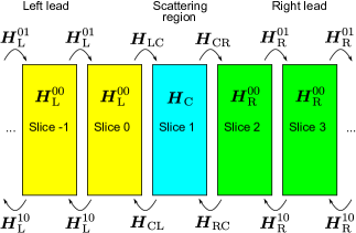
Figure 1: Schematic of the scattering system (left lead, scattering region and right lead) and the submatrices associated with each slice or principal layer which represents the set of atomic degrees of freedom for a block row in Eq. (1). The left and right lead each consist of a semi-infinite one-dimensional array of identical slices while the scattering region corresponds to the interface.

In our scheme, as shown in Fig. 1, the system is partitioned into three subsystems: (1) the left lead, (2) the scattering region and (3) the right lead. The leads are identified with the physical bulk lattices while the scattering region contains the interface. Each lead consists of a semi-infinite one-dimensional array of identical slices (or principal layers) while the scattering region is considered a slice by itself. Hence, the entire system has an infinite number of slices, each of which can be indexed by an integer. The index convention used in this paper is one in which the index increases as one goes from left to right. We define the scattering region as slice $1$ while the principal layers in the left and right lead are enumerated $-\infty,\ldots,0$ and $2,\ldots,+\infty$, respectively.

Formally, the lattice dynamical properties of the system are determined by the mass-normalized force-constant matrix $\mathbf{H}$ which represents the harmonic coupling of the entire system and has the block-tridiagonal structure,

$$\mathbf{H}=\left(\begin{array}[]{ccccccc}\ddots&\ddots\\ \ddots&\boldsymbol{H}_{\text{L}}^{00}&\boldsymbol{H}_{\text{L}}^{01}\\ &\boldsymbol{H}_{\text{L}}^{10}&\boldsymbol{H}_{\text{L}}^{00}&\boldsymbol{H}_{\text{LC}}\\ &&\boldsymbol{H}_{\text{CL}}&\boldsymbol{H}_{\text{C}}&\boldsymbol{H}_{\text{CR}}\\ &&&\boldsymbol{H}_{\text{RC}}&\boldsymbol{H}_{\text{R}}^{00}&\boldsymbol{H}_{\text{R}}^{01}\\ &&&&\boldsymbol{H}_{\text{R}}^{10}&\boldsymbol{H}_{\text{R}}^{00}&\ddots\\ &&&&&\ddots&\ddots\end{array}\right)$$ (1)

where $\boldsymbol{H}_{\text{C}}$, and $\boldsymbol{H}_{\text{CL}}$ ($\boldsymbol{H}_{\text{CR}}$) are respectively the force-constant submatrices corresponding to the interface region and the coupling between the interface region and the semi-infinite left (right) lead. We can associate each slice in Fig. 1 with a block row in $\mathbf{H}$. In the standard AGF setup, the block row submatrices $\boldsymbol{H}_{\alpha}^{00}$ and $\boldsymbol{H}_{\alpha}^{01}$, where $\alpha=\text{L}$ and $\alpha=\text{R}$ for the left and right lead, respectively, characterize the lead phonons. If we set the slices to be large enough so that only adjacent slices can couple, then $\boldsymbol{H}_{\alpha}^{00}$ corresponds to the force-constant matrix for each slice while $\boldsymbol{H}_{\alpha}^{01}$ ($\boldsymbol{H}_{\alpha}^{10}$) corresponds to the harmonic coupling between each slice and the slice to its right (left) in the lead. In the rest of the paper, we reserve $\alpha$ as the dummy variable for distinguishing the leads, with $\alpha=\text{L}$ and $\alpha=\text{R}$ representing the left and right lead, respectively.

We note here that in spite of the infinite number of slices making up the system, only a finite set of unique force-constant matrices ($\boldsymbol{H}_{\text{C}}$, $\boldsymbol{H}_{\text{CL}}$, $\boldsymbol{H}_{\text{CR}}$, $\boldsymbol{H}_{\text{L}}^{00}$, $\boldsymbol{H}_{\text{L}}^{01}$, $\boldsymbol{H}_{\text{R}}^{00}$ and $\boldsymbol{H}_{\text{R}}^{01}$) are needed as inputs for the AGF calculation because the leads are made up of identical slices and the Hermiticity of $\mathbf{H}$ implies that $\boldsymbol{H}_{\text{LC}}=(\boldsymbol{H}_{\text{CL}})^{\dagger}$ and $\boldsymbol{H}_{\text{RC}}=(\boldsymbol{H}_{\text{CR}})^{\dagger}$, and $\boldsymbol{H}_{\alpha}^{01}=(\boldsymbol{H}_{\alpha}^{10})^{\dagger}$. The periodic arraying of the slices in the leads means that each slice constitutes a unit cell and that the bulk phonon dispersion for the lead can be determined from the expression

$$\text{det}[\omega^{2}\boldsymbol{I}_{\alpha}-\boldsymbol{D}_{\alpha}(k)]=0\ ,$$ (2)

where $\boldsymbol{D}_{\alpha}(k)=\boldsymbol{H}_{\alpha}^{10}e^{-ika_{\alpha}}+\boldsymbol{H}_{\alpha}^{00}+\boldsymbol{H}_{\alpha}^{01}e^{ika_{\alpha}}$ is the dynamical matrix and $\boldsymbol{I}_{\alpha}$ is the identity matrix of the size as $\boldsymbol{H}_{\alpha}^{00}$; the variables $k$ and $a_{\alpha}$ represent the phonon wave vector and lattice constant in one dimension, respectively.

II.1.2 Total phonon transmission

In principle, the system dynamics are determined by the infinitely large $\mathbf{H}$ in Eq. (1). However, for the effective dynamics at a fixed frequency $\omega$, the lattice dynamics problem becomes more tractable as we need only to project the dynamics onto a finite portion of the system, (Wang et al., 2008; Mingo, 2009) corresponding to slices 0 to 2 in Fig. 1, to determine phonon transmission through the scattering region (slice 1). Hence, we use the submatrices in Eq. (1) to construct the effective harmonic matrix for this subsystem (Wang et al., 2008)

$$\mathbf{H}^{\prime}=\left(\begin{array}[]{ccc}\boldsymbol{H}_{\text{L}}^{\prime}&\boldsymbol{H}_{\text{LC}}^{\prime}&0\\ \boldsymbol{H}_{\text{CL}}^{\prime}&\boldsymbol{H}_{\text{C}}^{\prime}&\boldsymbol{H}_{\text{CR}}^{\prime}\\ 0&\boldsymbol{H}_{\text{RC}}^{\prime}&\boldsymbol{H}_{\text{R}}^{\prime}\end{array}\right)\ ,$$ (3)

where $\boldsymbol{H}_{\text{L}}^{\prime}=\boldsymbol{H}_{\text{L}}^{00}+\boldsymbol{H}_{\text{L}}^{10}\boldsymbol{g}_{\text{L},-}^{\text{ret}}\boldsymbol{H}_{\text{L}}^{01}$ and $\boldsymbol{H}_{\text{R}}^{\prime}=\boldsymbol{H}_{\text{R}}^{00}+\boldsymbol{H}_{\text{R}}^{01}\boldsymbol{g}_{\text{R},+}^{\text{ret}}\boldsymbol{H}_{\text{R}}^{10}$ represent the left and right edge, respectively while $\boldsymbol{H}_{\text{C}}^{\prime}=\boldsymbol{H}_{\text{C}}$ and $\boldsymbol{H}_{\text{CL/CR}}^{\prime}=\boldsymbol{H}_{\text{CL/CR}}=(\boldsymbol{H}_{\text{LC/RC}}^{\prime})^{\dagger}$ (see Fig. 2). The retarded surface Green’s functions $\boldsymbol{g}_{\text{L},-}^{\text{ret}}$ and $\boldsymbol{g}_{\text{R},+}^{\text{ret}}$ are given by

$$\boldsymbol{g}_{\alpha,-}^{\text{ret}}=[(\omega^{2}+i\eta)\boldsymbol{I}_{\alpha}-\boldsymbol{H}_{\alpha}^{00}-\boldsymbol{H}_{\alpha}^{10}\boldsymbol{g}_{\alpha,-}^{\text{ret}}\boldsymbol{H}_{\alpha}^{01}]^{-1}$$ (4a)

$$\boldsymbol{g}_{\alpha,+}^{\text{ret}}=[(\omega^{2}+i\eta)\boldsymbol{I}_{\alpha}-\boldsymbol{H}_{\alpha}^{00}-\boldsymbol{H}_{\alpha}^{01}\boldsymbol{g}_{\alpha,+}^{\text{ret}}\boldsymbol{H}_{\alpha}^{10}]^{-1}$$ (4b)

where $\eta$ is the small infinitesimal part that we add to $\omega^{2}$ to impose causality, and they are commonly generated using the decimation technique (Guinea et al., 1983) or by solving the generalized eigenvalue equation. (Wang et al., 2008; Sadasivam et al., 2017) Physically, Eq. (4a) is the retarded surface Green’s function for a decoupled semi-infinite lattice extending infinitely to the left (denoted by the ‘-’ in the subscript of $\boldsymbol{g}_{\alpha,-}^{\text{ret}}$) while Eq. (4b) is the corresponding surface Green’s function for a decoupled semi-infinite lattice extending infinitely to the right (denoted by the ‘+’ in the subscript of $\boldsymbol{g}_{\alpha,+}^{\text{ret}}$). In addition, the advanced surface Green’s functions can be obtained from the Hermitian conjugates of Eq. (4b), i.e. $\boldsymbol{g}_{\alpha,-}^{\text{adv}}=(\boldsymbol{g}_{\alpha,-}^{\text{ret}}){}^{\dagger}$ and $\boldsymbol{g}_{\alpha,+}^{\text{adv}}=(\boldsymbol{g}_{\alpha,+}^{\text{ret}})^{\dagger}$.

To find the phonon transmission through the interface, we compute the corresponding Green’s function for Eq. (3), $\boldsymbol{G}^{\text{ret}}=[(\omega^{2}+i\eta)\mathbf{I}^{\prime}-\mathbf{H}^{\prime}]^{-1}$ where $\mathbf{I}^{\prime}$ is an identity matrix of the same size as $\mathbf{H}^{\prime}$; the $\boldsymbol{G}^{\text{ret}}$ matrix can be partitioned into submatrices in the same manner as $\mathbf{H}^{\prime}$, i.e.

$$\boldsymbol{G}^{\text{ret}}=\left(\begin{array}[]{ccc}\boldsymbol{G}_{\text{L}}^{\text{ret}}&\boldsymbol{G}_{\text{LC}}^{\text{ret}}&\boldsymbol{G}_{\text{LR}}^{\text{ret}}\\ \boldsymbol{G}_{\text{CL}}^{\text{ret}}&\boldsymbol{G}_{\text{C}}^{\text{ret}}&\boldsymbol{G}_{\text{CR}}^{\text{ret}}\\ \boldsymbol{G}_{\text{RL}}^{\text{ret}}&\boldsymbol{G}_{\text{RC}}^{\text{ret}}&\boldsymbol{G}_{\text{R}}^{\text{ret}}\end{array}\right)\ .$$ (5)

In the original AGF method,(Zhang et al., 2007a; Wang et al., 2008) the phonon transmittance through the scattering region is given by the well-known Caroli formula: (Caroli et al., 1971; Zhang et al., 2007a; Wang et al., 2008)

$$\Xi(\omega)=\text{Tr}[\boldsymbol{\Gamma}_{\text{R}}\boldsymbol{G}_{\text{RL}}^{\text{ret}}\boldsymbol{\Gamma}_{\text{L}}(\boldsymbol{G}_{\text{RL}}^{\text{ret}})^{\dagger}]$$ (6)

where $\boldsymbol{\Gamma}_{\text{L}}=i\boldsymbol{H}_{\text{L}}^{10}(\boldsymbol{g}_{\text{L},-}^{\text{ret}}-\boldsymbol{g}_{\text{L},-}^{\text{adv}})\boldsymbol{H}_{\text{L}}^{01}$ and $\boldsymbol{\Gamma}_{\text{R}}=i\boldsymbol{H}_{\text{R}}^{01}(\boldsymbol{g}_{\text{R},+}^{\text{ret}}-\boldsymbol{g}_{\text{R},+}^{\text{adv}})\boldsymbol{H}_{\text{R}}^{10}$.

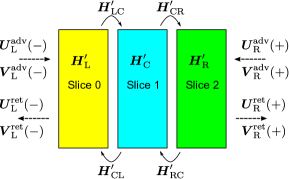
Figure 2: Schematic of the finite projected system in Eq. (3), consisting of the scattering region (slice $1$) and its terminated edges (slices $0$ and $2$). The frequency-dependent dynamics of the semi-infinite leads are implicitly included in $\boldsymbol{H}_{\text{L}}^{\prime}$ and $\boldsymbol{H}_{\text{R}}^{\prime}$ through the surface Green’s functions $\boldsymbol{g}_{\text{L},-}^{\text{ret}}$ and $\boldsymbol{g}_{\text{R},+}^{\text{ret}}$ from which we can derive the incoming and outgoing phonon modes [$\boldsymbol{U}_{\text{L}}^{\text{adv/ret}}(-)$ and $\boldsymbol{U}_{\text{R}}^{\text{adv/ret}}(+)$] and their group velocities [$\boldsymbol{V}_{\text{L}}^{\text{adv/ret}}(-)$ and $\boldsymbol{V}_{\text{R}}^{\text{adv/ret}}(+)$].

II.2 Phonon transmission, reflection and $S$-matrix

From the Green’s function $\boldsymbol{G}^{\text{ret}}$ in Eq. (5), we can use the traditional AGF method to compute the phonon transmittance $\Xi(\omega)$ which is the sum of the individual phonon transmission coefficients. (Huang et al., 2011; Ong and Zhang, 2015) A more explicit connection to conventional scattering theory may be made by noting that the transmission coefficients can be derived directly from the diagonal elements of the transmission matrix, (Fisher and Lee, 1981) which relates the amplitude of the incoming phonon flux to that of the outgoing forward-scattered (or transmitted) phonon flux and is computed numerically from $\boldsymbol{G}^{\text{ret}}$. (Ong and Zhang, 2015) However, this picture of the scattering process is incomplete as it does not treat the amplitude of the backward-scattered (or reflected) phonons and the trajectories of the phonons reflected from the interface. This suggests that a matrix analogous to the transmission matrix is needed for the backward component of the scattered phonons. To accomplish this, we introduce the reflection matrix and show how it can be computed efficiently by building on the technical ideas given in Ref. (Ong and Zhang, 2015). The reflection matrix for each lead can then be combined with the transmission matrices to form the $S$ matrix that governs overall phonon transmission and reflection at the interface.

II.2.1 Definition of transmission, absorption and reflection coefficients

Before we proceed, we clarify some of the terminology used in the following discussions. An incident or “incoming” phonon is one that has its group velocity pointing towards the interface and corresponds to the asymptotically free ($t\rightarrow-\infty$) bulk phonon state prior to scattering while an “outgoing” phonon is one that has its group velocity pointing away from the interface and corresponds to the asymptotically free ($t\rightarrow\infty$) bulk phonon state after scattering. There are two types of outgoing phonons: (1) the transmitted or forward-scattered phonons on the other side of the interface with a group velocity in the same direction as that of the incident phonon and (2) the reflected or backward-scattered phonons on the same side of the interface but with a group velocity opposite to that of the incident phonon. For example, an incoming phonon in the left lead propagating towards the interface has a positive group velocity. After colliding with the interface, the incoming phonon is scattered into a range of outgoing phonon states, transmitted and reflected, with a “scattering amplitude” and “transition probability” associated with each transition between the incoming phonon state and an outgoing phonon state.

We also use the transmission, absorption and reflection coefficients, which can be obtained from sums of the relevant transition probabilities, to characterize the loss and gain of energy by phonon channels. The transmission coefficient $\Xi$ associated with each incoming phonon channel is defined as the fraction of the energy flux lost by the incoming phonon channel across the interface to all the outgoing phonon channels on the other side. The absorption coefficient $\xi$ associated with each outgoing phonon channel is defined as the fraction of the energy flux gained by the outgoing phonon channel from all the incoming phonon channels across the interface. Similarly, we can also associate a reflection coefficient $\xi^{\prime}$ with each outgoing phonon channel, which we define as the fraction of the energy flux gained by the outgoing phonon channel from all the incoming channels on the same side of the interface.

II.2.2 Bloch matrices and bulk phonon eigenmodes

The advanced and retarded Bloch matrices (Ando, 1991; Khomyakov et al., 2005; Ong and Zhang, 2015) of the left and right lead, $\boldsymbol{F}_{\alpha}^{\text{adv/ret}}(+)$ and $\boldsymbol{F}_{\alpha}^{\text{adv/ret}}(-)$, describe their bulk translational symmetry along the direction of the heat flux and can be computed directly from the formulas:

$$\boldsymbol{F}_{\alpha}^{\text{adv/ret}}(+)=\boldsymbol{g}_{\alpha,+}^{\text{adv/ret}}\boldsymbol{H}_{\alpha}^{10}$$ (7a)

$$\boldsymbol{F}_{\alpha}^{\text{adv/ret}}(-)^{-1}=\boldsymbol{g}_{\alpha,-}^{\text{adv/ret}}\boldsymbol{H}_{\alpha}^{01}$$ (7b)

As pointed out in Ref. (Ong and Zhang, 2015), the bulk eigenmodes for the lead can be determined directly from the Bloch matrices:

$$\boldsymbol{F}_{\alpha}^{\text{adv/ret}}(+)\boldsymbol{U}_{\alpha}^{\text{adv/ret}}(+)=\boldsymbol{U}_{\alpha}^{\text{adv/ret}}(+)\boldsymbol{\Lambda}_{\alpha}^{\text{adv/ret}}(+)$$ (8a)

$$\boldsymbol{F}_{\alpha}^{\text{adv/ret}}(-)^{-1}\boldsymbol{U}_{\alpha}^{\text{adv/ret}}(-)=\boldsymbol{U}_{\alpha}^{\text{adv/ret}}(-)\boldsymbol{\Lambda}_{\alpha}^{\text{adv/ret}}(-)^{-1}$$ (8b)

where $\boldsymbol{U}_{\alpha}^{\text{ret}}(+)$ [$\boldsymbol{U}_{\alpha}^{\text{ret}}(-)$] is a matrix with its column vectors corresponding to the rightward-going (leftward-going) extended or rightward (leftward) decaying evanescent modes and has the form $\boldsymbol{U}_{\alpha}^{\text{ret}}=(\boldsymbol{e}_{1}\boldsymbol{e}_{2}\ldots\boldsymbol{e}_{N})$ where $\boldsymbol{e}_{n}$ is a normalized eigenvector of the Bloch matrix in the $n$-th column of $\boldsymbol{U}_{\alpha}^{\text{ret}}$ [$\boldsymbol{U}_{\alpha}^{\text{ret}}(-)$]. Similarly, $\boldsymbol{U}_{\alpha}^{\text{adv}}(-)$ [$\boldsymbol{U}_{\alpha}^{\text{adv}}(+)$] is a matrix with its column vectors corresponding to rightward-going (leftward-going) extended or leftward (rightward) decaying evanescent modes. The matrix $\boldsymbol{\Lambda}_{\alpha}^{\text{adv/ret}}(+)$ [$\boldsymbol{\Lambda}_{\alpha}^{\text{adv/ret}}(-)$] is a diagonal matrix with matrix elements of the form $e^{ik_{n}a}$ where $k_{n}$ is the phonon wave vector corresponding to the $n$-th column eigenvector in $\boldsymbol{U}_{\alpha}^{\text{adv/ret}}(+)$ [$\boldsymbol{U}_{\alpha}^{\text{adv/ret}}(-)$].

We note that because the Bloch matrices are not Hermitian, their eigenvectors are not necessarily orthogonal. This can pose a problem (Sadasivam et al., 2017) for transmission coefficient calculations when the eigenvectors have the same $k$ and are degenerate. This issue can be simply resolved by orthonormalizing the degenerate column eigenvectors in $\boldsymbol{U}_{\alpha}^{\text{adv/ret}}$ with a Gram-Schmidt procedure. (Arfken and Webber, 1995; Werneth et al., 2010) The final piece of ingredient needed for the following phonon scattering calculations is the diagonal velocity matrix (Khomyakov et al., 2005; Wang et al., 2008)

$$\boldsymbol{V}_{\alpha}^{\text{adv/ret}}(+)= \frac{ia_{\alpha}}{2\omega}[\boldsymbol{U}_{\alpha}^{\text{adv/ret}}(+)]^{\dagger}\boldsymbol{H}_{\alpha}^{01}[\boldsymbol{g}_{\alpha,+}^{\text{adv/ret}}-$$

$$(\boldsymbol{g}_{\alpha,+}^{\text{ret/adv}})^{\dagger}]\boldsymbol{H}_{\alpha}^{10}\boldsymbol{U}_{\alpha}^{\text{adv/ret}}(+)\ ,$$ (9)

which has group velocities of the eigenvectors in $\boldsymbol{U}_{\alpha}^{\text{adv/ret}}(+)$ as its diagonal elements. Likewise, $\boldsymbol{V}_{\alpha}^{\text{adv/ret}}(-)$ is defined as

$$\boldsymbol{V}_{\alpha}^{\text{adv/ret}}(-)= -\frac{ia_{\alpha}}{2\omega}[\boldsymbol{U}_{\alpha}^{\text{adv/ret}}(-)]^{\dagger}\boldsymbol{H}_{\alpha}^{10}[\boldsymbol{g}_{\alpha,-}^{\text{adv/ret}}-$$

$$(\boldsymbol{g}_{\alpha,-}^{\text{ret/adv}})^{\dagger}]\boldsymbol{H}_{\alpha}^{01}\boldsymbol{U}_{\alpha}^{\text{adv/ret}}(-)\ .$$ (10)

For evanescent modes, the group velocity is always zero while for propagating modes that contribute to the heat flux, the group velocity is positive (negative) in $\boldsymbol{V}_{\alpha}^{\text{ret}}(+)$ and $\boldsymbol{V}_{\alpha}^{\text{adv}}(-)$ [$\boldsymbol{V}_{\alpha}^{\text{ret}}(-)$ and $\boldsymbol{V}_{\alpha}^{\text{adv}}(+)$]. In addition, we define the diagonal matrices $\widetilde{\boldsymbol{V}}_{\alpha}^{\text{adv/ret}}(+)$ and $\widetilde{\boldsymbol{V}}_{\alpha}^{\text{adv/ret}}(-)$ in which their nonzero diagonal matrix elements are the inverse of those of $\boldsymbol{V}_{\alpha}^{\text{adv/ret}}(+)$ and $\boldsymbol{V}_{\alpha}^{\text{adv/ret}}(-),$ respectively. For each lead, we can also define the diagonal matrices

$$\boldsymbol{I}_{\alpha}^{\text{adv/ret}}(+)=\boldsymbol{V}_{\alpha}^{\text{adv/ret}}(+)\widetilde{\boldsymbol{V}}_{\alpha}^{\text{adv/ret}}(+)$$ (11a)

$$\boldsymbol{I}_{\alpha}^{\text{adv/ret}}(-)=\boldsymbol{V}_{\alpha}^{\text{adv/ret}}(-)\widetilde{\boldsymbol{V}}_{\alpha}^{\text{adv/ret}}(-)$$ (11b)

in which the $n$-th diagonal element equals $1$ if the $n$-th column of $\boldsymbol{U}_{\alpha}^{\text{adv/ret}}(+)$ and $\boldsymbol{U}_{\alpha}^{\text{adv/ret}}(-)$ corresponds to an extended mode and $0$ otherwise. Therefore, it follows from Eq. (11b ) that the number of rightward-going phonon channels $N_{\alpha}(+)$ and the number of leftward-going phonon channels $N_{\alpha}(-)$ are given by

$$N_{\alpha}(+)=\text{Tr}[\boldsymbol{I}_{\alpha}^{\text{ret}}(+)]=\text{Tr}[\boldsymbol{I}_{\alpha}^{\text{adv}}(-)]$$ (12a)

$$N_{\alpha}(-)=\text{Tr}[\boldsymbol{I}_{\alpha}^{\text{ret}}(-)]=\text{Tr}[\boldsymbol{I}_{\alpha}^{\text{adv}}(+)]\ .$$ (12b)

II.2.3 Phonon scattering: transmission

Now, let us consider the scattering problem for an incoming phonon from the left lead that is incident on the scattering region. In the $n=0$ slice at the edge of the left lead, the motion can be decomposed into two parts, i.e.

$$\boldsymbol{c}_{0}=\boldsymbol{c}_{0}(+)+\boldsymbol{c}_{0}(-)$$ (13)

where $\boldsymbol{c}_{0}(+)$ and $\boldsymbol{c}_{0}(-)$ respectively represent the rightward-going (incident) and leftward-going (reflected) components, while in the $n=2$ slice at the edge of the right lead, the motion is given by

$$\boldsymbol{c}_{2}=\boldsymbol{c}_{2}(+)\ ,$$ (14)

where the right-hand side represents a rightward-going (transmitted) wave which can be a linear combination of bulk right-lead phonon modes propagating away from the interface. Suppose the rightward-going component in Eq. (13) is a left-lead bulk phonon mode, i.e. $\boldsymbol{c}_{0}(+)=\boldsymbol{u}_{\text{L},n}(k,\omega)$ where $n$ and $k$ are the phonon polarization index and wave vector, respectively. Then, it can be shown (Khomyakov et al., 2005) that the transmitted wave $\boldsymbol{c}_{2}(+)$ in the right lead is related to the incident wave $\boldsymbol{c}_{0}(+)$ from the right lead, via the expression

$$\boldsymbol{c}_{2}=\boldsymbol{G}_{\text{RL}}^{\text{ret}}\boldsymbol{Q}_{\text{L}}\boldsymbol{u}_{\text{L},n}(k,\omega)$$ (15)

where

$$\boldsymbol{Q}_{\alpha}= (\omega^{2}+i\eta)\boldsymbol{I}_{\alpha}-\boldsymbol{H}_{\alpha}^{00}$$

$$-\boldsymbol{H}_{\alpha}^{10}\boldsymbol{g}_{\alpha,-}^{\text{ret}}(\omega)\boldsymbol{H}_{\alpha}^{01}-\boldsymbol{H}_{\alpha}^{01}\boldsymbol{g}_{\alpha,+}^{\text{ret}}(\omega)\boldsymbol{H}_{\alpha}^{10}$$ (16)

and $\boldsymbol{Q}_{\alpha}^{-1}$ is the bulk Green’s function of the $\alpha$ lead. The expression in Eq. (15) can be expressed as a linear combination of transmitted right-lead phonon modes $\boldsymbol{u}_{\text{R},m}(k_{m},\omega)$, i.e. $\boldsymbol{c}_{2}=\sum_{m}\boldsymbol{u}_{\text{R},m}(k_{m},\omega)\tau_{mn}$, where $\tau_{mn}$ is the linear coefficient and forms the matrix elements of the transmission matrix $\boldsymbol{\tau}$, where

$$\boldsymbol{\tau}=[\boldsymbol{U}_{\text{R}}^{\text{ret}}(+)]^{-1}\boldsymbol{G}_{\text{RL}}^{\text{ret}}\boldsymbol{Q}_{\text{L}}\boldsymbol{U}_{\text{L}}^{\text{ret}}(+)\ .$$ (17)

The flux-normalized transmission matrix is $\boldsymbol{t}_{\text{RL}}=[\boldsymbol{V}_{\text{R}}^{\text{ret}}(+)]^{\nicefrac{{1}}{{2}}}\boldsymbol{\tau}[\widetilde{\boldsymbol{V}}_{\text{L}}^{\text{ret}}(+)]^{\nicefrac{{1}}{{2}}}$, which we can rewrite as (Ong and Zhang, 2015)

$$\boldsymbol{t}_{\text{RL}}= \frac{2i\omega}{\sqrt{a_{\text{R}}a_{\text{L}}}}[\boldsymbol{V}_{\text{R}}^{\text{ret}}(+)]^{\nicefrac{{1}}{{2}}}[\boldsymbol{U}_{\text{R}}^{\text{ret}}(+)]^{-1}$$

$$\times\boldsymbol{G}_{\text{RL}}^{\text{ret}}[\boldsymbol{U}_{\text{L}}^{\text{adv}}(-)^{\dagger}]^{-1}[\boldsymbol{V}_{\text{L}}^{\text{adv}}(-)]^{\nicefrac{{1}}{{2}}}\ .$$ (18)

Each row of $\boldsymbol{t}_{\text{RL}}$ corresponds to either a transmitted right-lead extended or evanescent mode. For an outgoing evanescent mode, the row elements and group velocity, given by the diagonal element of $\boldsymbol{V}_{\text{R}}^{\text{ret}}(+)$, are zero. Conversely, each column of of $\boldsymbol{t}_{\text{RL}}$ corresponds to either an incident left-lead extended or evanescent mode, and the column elements and group velocity of the evanescent modes, given by the diagonal element of $\boldsymbol{V}_{\text{L}}^{\text{adv}}(-)$, are zero. If the $m$-th row and $n$-th column of $\boldsymbol{t}_{\text{RL}}$correspond to extended transmitted and incident modes, then $|[\boldsymbol{t}_{\text{RL}}]_{mn}|^{2}$ gives us the probability that incident left-lead phonon is transmitted across the interface into the right-lead phonon. Similarly, we can define the flux-normalized transmission matrix for phonon transmission from the right to the left lead:

$$\boldsymbol{t}_{\text{LR}}= \frac{2i\omega}{\sqrt{a_{\text{L}}a_{\text{R}}}}[\boldsymbol{V}_{\text{L}}^{\text{ret}}(-)]^{\nicefrac{{1}}{{2}}}[\boldsymbol{U}_{\text{L}}^{\text{ret}}(-)]^{-1}$$

$$\times\boldsymbol{G}_{\text{LR}}^{\text{ret}}[\boldsymbol{U}_{\text{R}}^{\text{adv}}(+)^{\dagger}]^{-1}[\boldsymbol{V}_{\text{R}}^{\text{adv}}(+)]^{\nicefrac{{1}}{{2}}}\ .$$ (19)

II.2.4 Phonon scattering: reflection

Like in Eq. (15), we can describe the motion in slice 0 in terms of the incident wave, i.e. $\boldsymbol{c}_{0}=\boldsymbol{G}_{\text{L}}^{\text{ret}}\boldsymbol{Q}_{\text{L}}\boldsymbol{u}_{\text{L},n}(k,\omega)$. It follows that the reflected component is $\boldsymbol{c}_{0}(-)=\boldsymbol{c}_{0}-\boldsymbol{c}_{0}(+)=(\boldsymbol{G}_{\text{L}}^{\text{ret}}-\boldsymbol{Q}_{\text{L}}^{-1})\boldsymbol{Q}_{\text{L}}\boldsymbol{u}_{\text{L},n}(k,\omega)$. Therefore, the flux-normalized reflection matrix, which gives the scattering amplitude between leftward-going (reflected) and rightward-going (incident) states in the left lead, can be defined as:

$$\boldsymbol{r}_{\text{LL}}= \frac{2i\omega}{a_{\text{L}}}[\boldsymbol{V}_{\text{L}}^{\text{ret}}(-)]^{\nicefrac{{1}}{{2}}}[\boldsymbol{U}_{\text{L}}^{\text{ret}}(-)]^{-1}$$

$$\times(\boldsymbol{G}_{\text{L}}^{\text{ret}}-\boldsymbol{Q}_{\text{L}}^{-1})[\boldsymbol{U}_{\text{L}}^{\text{adv}}(-)^{\dagger}]^{-1}[\boldsymbol{V}_{\text{L}}^{\text{adv}}(-)]^{\nicefrac{{1}}{{2}}}\ .$$ (20)

The corresponding expression for phonon reflection in the right lead can be similarly defined as

$$\boldsymbol{r}_{\text{RR}}= \frac{2i\omega}{a_{\text{R}}}[\boldsymbol{V}_{\text{R}}^{\text{ret}}(+)]^{\nicefrac{{1}}{{2}}}[\boldsymbol{U}_{\text{R}}^{\text{ret}}(+)]^{-1}$$

$$\times(\boldsymbol{G}_{\text{R}}^{\text{ret}}-\boldsymbol{Q}_{\text{R}}^{-1})[\boldsymbol{U}_{\text{R}}^{\text{adv}}(+)^{\dagger}]^{-1}[\boldsymbol{V}_{\text{R}}^{\text{adv}}(+)]^{\nicefrac{{1}}{{2}}}\ ,$$ (21)

which gives the scattering amplitude between rightward-going (reflected) and leftward-going (incident) states in the right lead.

II.2.5 Phonon transmission and reflection matrices

Given Eqs. (18) to (21), we can construct the rationalized smaller matrices $\bar{\boldsymbol{t}}_{\text{RL}}$, $\bar{\boldsymbol{t}}_{\text{LR}}$, $\bar{\boldsymbol{r}}_{\text{LL}}$ and $\bar{\boldsymbol{r}}_{\text{RR}}$ from $\boldsymbol{t}_{\text{RL}}$, $\boldsymbol{t}_{\text{LR}}$, $\boldsymbol{r}_{\text{LL}}$ and $\boldsymbol{r}_{\text{RR}}$ by deleting the matrix rows and columns corresponding to evanescent states. This is done numerically by inspecting each diagonal element of $\boldsymbol{I}_{\alpha}^{\text{adv/ret}}(\pm)$ of Eq. (11b), which is either equal to 0 (evanescent) or 1 (extended), and removing the corresponding columns or rows when $[\boldsymbol{I}_{\alpha}^{\text{adv/ret}}(\pm)]_{nn}=0$. For example, to find $\bar{\boldsymbol{t}}_{\text{RL}}$, we inspect $\boldsymbol{I}_{\text{R}}^{\text{ret}}(+)$ for row deletion and $\boldsymbol{I}_{\text{L}}^{\text{adv}}(-)$ for column deletion in $\boldsymbol{t}_{\text{RL}}$. Hence, $\bar{\boldsymbol{t}}_{\text{RL}}$ is an $N_{\text{R}}(+)\times N_{\text{L}}(+)$ matrix. Similarly, we can also define the rationalized smaller matrices $\bar{\boldsymbol{\Lambda}}_{\alpha}^{\text{adv/ret}}(+)$ by deleting the rows and columns associated with evanescent modes from $\boldsymbol{\Lambda}_{\alpha}^{\text{adv/ret}}(\pm)$ in Eq. (8b).

The transmission coefficient of the $n$-th incoming phonon channel in the left lead is defined as the $n$-th diagonal element of $\bar{\boldsymbol{t}}_{\text{RL}}^{\dagger}\bar{\boldsymbol{t}}_{\text{RL}}$, i.e.

$$\Xi_{\text{L},n}=[\bar{\boldsymbol{t}}_{\text{RL}}^{\dagger}\bar{\boldsymbol{t}}_{\text{RL}}]_{nn}\ ,$$ (22)

which is equal to the fraction of its energy flux transmitted across the interface, and its wave vector $k_{n}$ can be determined from $[\bar{\boldsymbol{\Lambda}}_{\text{L}}^{\text{adv}}(-)]_{nn}=e^{ik_{n}a_{\text{L}}}$ or $k_{n}=\frac{1}{a_{\text{L}}}\cos^{-1}\text{Re}[\bar{\boldsymbol{\Lambda}}_{\text{L}}^{\text{adv}}(-)]_{nn}$. For the reflected modes, the reflection coefficient of the $m$-th outgoing leftward-going mode in the left lead is given by the $m$-th diagonal element of $\bar{\boldsymbol{r}}_{\text{LL}}\bar{\boldsymbol{r}}_{\text{LL}}^{\dagger}$, i.e.

$$\xi_{\text{L},m}^{\prime}=[\bar{\boldsymbol{r}}_{\text{LL}}\bar{\boldsymbol{r}}_{\text{LL}}^{\dagger}]_{mm}\ ,$$ (23)

with its phonon wave vector $k_{m}$ given by $k_{m}=\frac{1}{a_{\text{L}}}\cos^{-1}\text{Re}[\bar{\boldsymbol{\Lambda}}_{\text{L}}^{\text{ret}}(-)]_{mm}$, while the absorption coefficient of the $l$-th outgoing rightward-going mode in the right lead is given by the $l$-th diagonal element of $\bar{\boldsymbol{t}}_{\text{RL}}\bar{\boldsymbol{t}}_{\text{RL}}^{\dagger}$, i.e.

$$\xi_{\text{R},l}=[\bar{\boldsymbol{t}}_{\text{RL}}\bar{\boldsymbol{t}}_{\text{RL}}^{\dagger}]_{ll}\ ,$$ (24)

with its phonon wave vector $k_{l}$ given by $k_{l}=\frac{1}{a_{\text{R}}}\cos^{-1}\text{Re}[\bar{\boldsymbol{\Lambda}}_{\text{R}}^{\text{ret}}(+)]_{ll}$.

The transmission coefficient for the $n$-th incoming phonon channel in the right lead ($\Xi_{\text{R},n}$), the absorption coefficient of the $l$-th outgoing phonon channel in the left lead ($\xi_{\text{L},l}$ ) and the reflection coefficient of the $m$-th outgoing phonon channel in the right lead ($\xi_{\text{R},m}^{\prime}$) can be similarly defined like in Eqs. (22) to (24), and their formulas are summarized in Table 1. It should also be noted that for $\alpha=\text{L},\text{R}$,

$$\xi_{\alpha,m}+\xi_{\alpha,m}^{\prime}=1$$ (25)

which physically means that the sum of the energy flux fractions from absorption and reflection equals unity, consistent with the conservation of energy. In addition, we remark that the phonon transmittance can be expressed as the sum of the transmission [Eq. (26a)] or absorption [Eq. (26b)] coefficients of either lead, i.e.

$$\Xi(\omega) =\sum_{n=1}^{N_{\text{L}}(+)}\Xi_{\text{L},n}=\sum_{m=1}^{N_{\text{R}}(-)}\Xi_{\text{R},m}\$$ (26a)

$$=\sum_{n=1}^{N_{\text{L}}(-)}\xi_{\text{L},n}=\sum_{m=1}^{N_{\text{R}}(+)}\xi_{\text{R},m}\ .$$ (26b)

II.2.6 Phonon scattering specularity

With our method, the phonon scattering specularity parameter, which measures the ‘smoothness’ of a surface, can be extracted directly from the reflection matrices $\bar{\boldsymbol{r}}_{\text{LL}}$ and $\bar{\boldsymbol{r}}_{\text{RR}}$. Here, we discuss briefly the meaning of phonon specularity and how it is computed in the AGF-based $S$-matrix approach. In Ref. (Ziman, 1960), the specularity parameter is simply defined as the proportion of the intensity of the incident wave that remains in the outgoing wave in the specular direction, with the effects of polarization conversion ignored and the rest of the intensity assumed to be redistributed equally in all directions. In our $S$-matrix approach, we adopt a similar definition for atomistic phonon scattering specularity $\mathcal{P}$ by taking it to be the intensity proportion that is scattered to the specularly reflected outgoing channel, which we define as the outgoing phonon channel with the longitudinal wave vector $k_{\bar{n}}=-k_{n}$ and of the same polarization. However, we caution that this definition of specularity does not necessarily imply that the remainder is equally distributed in the rest of the outgoing channels, i.e. the absence of specularity does not correspond to diffusive scattering.

In the case of total phonon reflection in the left lead, the specularity parameter $\mathcal{P}_{\text{L}}(k_{n})$ for the incoming left-lead phonon at $k_{n}$ is determined by its transition probability to the outgoing phonon channel at $k_{\bar{n}}$, i.e.

$$\mathcal{P}_{\text{L}}(k_{n})=|[\bar{\boldsymbol{r}}_{\text{LL}}^{\dagger}]_{n\bar{n}}|^{2}\ .$$ (27)

The expression in Eq. (27) satisfies the requirement that $\mathcal{P}=1$ for fully specular reflection and in the limit that the number of channels goes to infinity, $\mathcal{P}=0$ for fully diffusive scattering. (Ziman, 1960) In the more general case of partial phonon reflection and transmission at an interface, the specularity parameter for the mode at $k_{n}$ in Eq. (27) has to be normalized by the overall probability of its phonon reflection, giving us

$$\mathcal{P}_{\text{L}}(k_{n})=\frac{|[\bar{\boldsymbol{r}}_{\text{LL}}^{\dagger}]_{n\bar{n}}|^{2}}{\sum_{m}|[\bar{\boldsymbol{r}}_{\text{LL}}^{\dagger}]_{nm}|^{2}}=\frac{|[\bar{\boldsymbol{r}}_{\text{LL}}^{\dagger}]_{n\bar{n}}|^{2}}{[\bar{\boldsymbol{r}}_{\text{LL}}^{\dagger}\bar{\boldsymbol{r}}_{\text{LL}}]_{nn}}\ .$$ (28)

Similarly, the specularity parameter for an incoming right-lead phonon with the wave vector $k_{m}$ is $\mathcal{P}_{\text{R}}(k_{m})=|[\bar{\boldsymbol{r}}_{\text{RR}}^{\dagger}]_{m\bar{m}}|^{2}/[\bar{\boldsymbol{r}}_{\text{RR}}^{\dagger}\bar{\boldsymbol{r}}_{\text{RR}}]_{mm}\ .$

Variable	Formula	Phonon wave vector
Incoming left-lead phonon transmission coefficient	$\Xi_{\text{L},n}=[\bar{\boldsymbol{t}}_{\text{RL}}^{\dagger}\bar{\boldsymbol{t}}_{\text{RL}}]_{nn}$	$k_{n}=\frac{1}{a_{\text{L}}}\cos^{-1}\text{Re}[\bar{\boldsymbol{\Lambda}}_{\text{L}}^{\text{adv}}(-)]_{nn}$
Outgoing right-lead phonon absorption coefficient	$\xi_{\text{R},n}=[\bar{\boldsymbol{t}}_{\text{RL}}\bar{\boldsymbol{t}}_{\text{RL}}^{\dagger}]_{nn}$	$k_{n}=\frac{1}{a_{\text{R}}}\cos^{-1}\text{Re}[\bar{\boldsymbol{\Lambda}}_{\text{R}}^{\text{ret}}(+)]_{nn}$
Outgoing left-lead phonon reflection coefficient	$\xi_{\text{L},n}^{\prime}=[\bar{\boldsymbol{r}}_{\text{LL}}\bar{\boldsymbol{r}}_{\text{LL}}^{\dagger}]_{nn}$	$k_{n}=\frac{1}{a_{\text{L}}}\cos^{-1}\text{Re}[\bar{\boldsymbol{\Lambda}}_{\text{L}}^{\text{ret}}(-)]_{nn}$
Incoming right-lead phonon transmission coefficient	$\Xi_{\text{R},n}=[\bar{\boldsymbol{t}}_{\text{LR}}^{\dagger}\bar{\boldsymbol{t}}_{\text{LR}}]_{nn}$	$k_{n}=\frac{1}{a_{\text{R}}}\cos^{-1}\text{Re}[\bar{\boldsymbol{\Lambda}}_{\text{R}}^{\text{adv}}(+)]_{nn}$
Outgoing left-lead phonon absorption coefficient	$\xi_{\text{L},n}=[\bar{\boldsymbol{t}}_{\text{LR}}\bar{\boldsymbol{t}}_{\text{LR}}^{\dagger}]_{nn}$	$k_{n}=\frac{1}{a_{\text{L}}}\cos^{-1}\text{Re}[\bar{\boldsymbol{\Lambda}}_{\text{L}}^{\text{ret}}(-)]_{nn}$
Outgoing right-lead phonon reflection coefficient	$\xi_{\text{R},n}^{\prime}=[\bar{\boldsymbol{r}}_{\text{RR}}\bar{\boldsymbol{r}}_{\text{RR}}^{\dagger}]_{nn}$	$k_{n}=\frac{1}{a_{\text{R}}}\cos^{-1}\text{Re}[\bar{\boldsymbol{\Lambda}}_{\text{R}}^{\text{ret}}(+)]_{nn}$

Table 1: Summary of formulas for the phonon mode transmission, absorption and reflection coefficients. The term ‘incoming’ describes a phonon moving towards the interface while ‘outgoing’ refers to phonons moving away from the interface.

II.2.7 $S$-matrix description of phonon scattering

Given $\bar{\boldsymbol{t}}_{\text{RL}}$, $\bar{\boldsymbol{t}}_{\text{LR}}$, $\bar{\boldsymbol{r}}_{\text{LL}}$ and $\bar{\boldsymbol{r}}_{\text{RR}}$, we can define the $S$ matrix

$$\boldsymbol{S}=\left(\begin{array}[]{cc}\bar{\boldsymbol{r}}_{\text{LL}}&\bar{\boldsymbol{t}}_{\text{LR}}\\ \bar{\boldsymbol{t}}_{\text{RL}}&\bar{\boldsymbol{r}}_{\text{RR}}\end{array}\right)\ ,$$ (29)

which connects the amplitudes of the scattered (reflected and transmitted) bulk phonons to the incident bulk phonons and is unitary if the system possesses time-reversal symmetry, i.e. $\boldsymbol{S}\boldsymbol{S}^{\dagger}=\boldsymbol{S}^{\dagger}\boldsymbol{S}=\boldsymbol{I}_{p}$ where $\boldsymbol{I}_{p}$ is an identity matrix of the same size as $\boldsymbol{S}$. The unitarity of $\boldsymbol{S}$ allows us to derive several identities involving $\bar{\boldsymbol{t}}_{\text{RL}}$, $\bar{\boldsymbol{t}}_{\text{LR}}$, $\bar{\boldsymbol{r}}_{\text{LL}}$ and $\bar{\boldsymbol{r}}_{\text{RR}}$. Equations (12b) and (29) imply that

$$N_{\text{L}}(+)+N_{\text{R}}(-)=N_{\text{L}}(-)+N_{\text{R}}(+)\ ,$$ (30)

i.e. the total number of incoming phonon channels is equal to the total number of outgoing phonon channels. It follows from Eqs. (29) and (25) that

$$\left\{\begin{array}[]{c}N_{\text{L}}(+)\\ N_{\text{L}}(-)\end{array}\right\}=\left\{\begin{array}[]{c}\text{Tr}(\bar{\boldsymbol{r}}_{\text{LL}}^{\dagger}\bar{\boldsymbol{r}}_{\text{LL}}+\bar{\boldsymbol{t}}_{\text{RL}}^{\dagger}\bar{\boldsymbol{t}}_{\text{RL}})\\ \text{Tr}(\bar{\boldsymbol{r}}_{\text{LL}}\bar{\boldsymbol{r}}_{\text{LL}}^{\dagger}+\bar{\boldsymbol{t}}_{\text{LR}}\bar{\boldsymbol{t}}_{\text{LR}}^{\dagger})\end{array}\right\}$$ (31)

and $N_{\text{L}}(+)=N_{\text{L}}(-)$, i.e., the number of leftward-going bulk phonon channels is equal to the number of rightward-going bulk phonon channels in the left lead. Similarly, we also have

$$\left\{\begin{array}[]{c}N_{\text{R}}(-)\\ N_{\text{R}}(+)\end{array}\right\}=\left\{\begin{array}[]{c}\text{Tr}(\bar{\boldsymbol{r}}_{\text{RR}}^{\dagger}\bar{\boldsymbol{r}}_{\text{RR}}+\bar{\boldsymbol{t}}_{\text{LR}}^{\dagger}\bar{\boldsymbol{t}}_{\text{LR}})\\ \text{Tr}(\bar{\boldsymbol{r}}_{\text{RR}}\bar{\boldsymbol{r}}_{\text{RR}}^{\dagger}+\bar{\boldsymbol{t}}_{\text{RL}}\bar{\boldsymbol{t}}_{\text{RL}}^{\dagger})\end{array}\right\}$$ (32)

and $N_{\text{R}}(-)=N_{\text{R}}(+)$. Equations (31) and (32) also allow us to establish the general reciprocity relationship, (Maznev et al., 2013)

$$\text{Tr}(\bar{\boldsymbol{t}}_{\text{RL}}\bar{\boldsymbol{t}}_{\text{RL}}^{\dagger})=\text{Tr}(\bar{\boldsymbol{t}}_{\text{LR}}\bar{\boldsymbol{t}}_{\text{LR}}^{\dagger})\ ,$$ (33)

or that the total rightward-going phonon transmission is equal to total leftward-going phonon transmission. They also imply that the phonon transmittance is bounded by the finite number of channels, i.e., $\Xi(\omega)\leq\text{min}\left(N_{\text{L}}(+),N_{\text{R}}(-)\right)\ .$

III Example with carbon nanotube junction

We illustrate the method by simulating phonon scattering at the armchair junction between two isotopically different but structurally identical (8,8) carbon nanotubes, as can be seen in Fig. 3(a), with the left one (‘CNT-12’) consisting of ¹²C atoms and the right one (‘CNT-24’) of ²⁴C atoms which have twice the mass of ¹²C atoms. The greater atomic mass of the ²⁴C atom doubles the mass density of CNT-24 and hence rescales its phonon frequencies by a factor of $\frac{1}{\sqrt{2}}$, introducing a difference in the polarization and distribution of phonon channels on either side of the junction at each frequency $\omega$. However, the phonon dispersion ($\omega$ vs. $k$) curves in CNT-24 are identical in shape to those of CNT-12 apart from the difference in frequency scaling. Thus, each phonon branch or ‘subband’ in CNT-12, which depends on polarization and angular symmetry, (Dobardžić et al., 2003) has a unique image subband in CNT-24 and as we shall show later, this simplifies our analysis of the polarization dependence of phonon scattering. Although ²⁴C atoms do not exist, this fictitious system is sufficiently realistic to contain the essential physics of phonon scattering by an interface as well as to illustrate key concepts introduced in the previous section.

III.1 Calculation details

We build the carbon nanotube (CNT) and optimize its structure in GULP (Gale and Rohl, 2003) using the Tersoff potential (Tersoff, 1988) parameters from Ref. (Lindsay and Broido, 2010). The force-constant matrices for the left and right leads ($\boldsymbol{H}_{\text{L}}^{00}$, $\boldsymbol{H}_{\text{L}}^{01}$, $\boldsymbol{H}_{\text{R}}^{00}$ and $\boldsymbol{H}_{\text{R}}^{01}$) are also computed in GULP. In our CNT structure, the interatomic interactions are sufficiently short-range so that the primitive unit cells correspond to the individual slices in our AGF calculation. At each frequency ($\omega$) point, we use the force-constant matrices to find the surface Green’s function $\boldsymbol{g}_{\text{R},+}^{\text{ret}}$ and $\boldsymbol{g}_{\text{L},-}^{\text{ret}}$, from which we determine $\mathbf{H}^{\prime}$ and $\boldsymbol{G}^{\text{ret}}$ using Eqs. (3) and (5). Using Eqs. (7b) and (8b), we also calculate the incoming phonon modes $\boldsymbol{U}_{\text{L}}^{\text{adv}}(-)$ and $\boldsymbol{U}_{\text{R}}^{\text{adv}}(+)$ and the outgoing phonon modes $\boldsymbol{U}_{\text{L}}^{\text{ret}}(-)$ and $\boldsymbol{U}_{\text{R}}^{\text{ret}}(+)$ as well as their associated velocity matrices,$\boldsymbol{V}_{\text{L}}^{\text{adv}}(-)$, $\boldsymbol{V}_{\text{R}}^{\text{adv}}(+)$, $\boldsymbol{V}_{\text{L}}^{\text{ret}}(-)$ and $\boldsymbol{V}_{\text{R}}^{\text{ret}}(+)$. The surface Green’s functions $\boldsymbol{g}_{\text{R},-}^{\text{ret}}$ and $\boldsymbol{g}_{\text{L},+}^{\text{ret}}$ are also computed and combined with $\boldsymbol{g}_{\text{R},+}^{\text{ret}}$ and $\boldsymbol{g}_{\text{L},-}^{\text{ret}}$ to find $\boldsymbol{Q}_{\text{R}}$ and $\boldsymbol{Q}_{\text{L}}$. Finally, these matrix variables are collected and used to compute the transmission and reflection matrices ($\boldsymbol{t}_{\text{RL}}$, $\boldsymbol{t}_{\text{LR}}$, $\boldsymbol{r}_{\text{LL}}$ and $\boldsymbol{r}_{\text{RR}}$ ) in Eqs. (18) to (21). We then eliminate the non-physical matrix rows and columns from them to obtain $\bar{\boldsymbol{t}}_{\text{RL}}$, $\bar{\boldsymbol{t}}_{\text{LR}}$, $\bar{\boldsymbol{r}}_{\text{LL}}$ and $\bar{\boldsymbol{r}}_{\text{RR}}$ which constitute the $S$ matrix in Eq. (29). The transmission, absorption, and reflection coefficients of the phonon channels for each CNT are computed, using Eqs. (22) to (24).

III.2 Transmission, absorption and reflection coefficients

We analyze the distribution of the transmission, absorption and reflection coefficients for the incident phonon flux from CNT-12 to CNT-24. Figure 3(b) shows the reflection coefficient distribution [$\xi_{\text{L},n}^{\prime}$ for $n=1,\ldots,N_{\text{L}}(-)$] for the outgoing leftward-going phonon modes while Fig. 3(c) shows the transmission coefficient distribution [$\Xi_{\text{L},n}$ for $n=1,\ldots,N_{\text{L}}(+)$] for the incoming rightward-going phonon modes in CNT-12. On the other side of the interface, the absorption coefficient distribution [$\xi_{\text{R},n}$ for $n=1,\ldots,N_{\text{R}}(+)$] for the outgoing rightward-going phonon modes in CNT-24 is shown in Fig. 3(d). We also plot the phonon dispersion curves for CNT-12 and CNT-24 in Fig. 3 over the frequency range between 0 and 100 meV, with the individual phonon branches (Dresselhaus and Eklund, 2000) clearly visible. In each spectrum, we note that only half of the points on the dispersion curves contribute to the transmission or absorption/reflection because half of the modes are either leftward or rightward-going. Thus, only half of the phonon channels can contribute to the phonon transmission or reflection at any frequency.

Figure 3(c) shows that at low frequencies ($\omega<20$ meV), the transmission coefficients ($\Xi_{\text{L},n}$) of all the incoming phonon modes are very close to unity, i.e. the phonon modes in CNT-12 are nearly perfectly transmitted across the interface. Conversely, the reflection coefficients ($\xi_{\text{L},n}^{\prime}$) of the corresponding outgoing phonon modes in Fig. 3(b) are close to zero at low frequencies. A comparison of Figs. 3(b) and (c) shows that each reflected phonon mode at $k_{i}$ with a reflection coefficient of $\xi_{\text{L},i}^{\prime}$ in Fig. 3(b) corresponds symmetrically to a transmitted phonon mode at $k_{j}=-k_{i}$ with a transmission coefficient of $\Xi_{\text{L},j}=1-\xi_{\text{L},i}^{\prime}$ in Fig. 3(c). In CNT-24 [Fig. 3(d)], the absorption coefficient spectrum ($\xi_{\text{R},n}$) for the outgoing phonon modes reveals that many of the rightward-going phonon channels have an absorption coefficient close to zero even at low frequencies although others have an absorption coefficient close to unity, indicating that there are preferred outgoing channels and subbands for phonon absorption. The presence of these $\xi_{\text{R},n}\sim 0$ channels is because at the same frequency ($\omega$), there are generally more phonon channels in CNT-24 than in CNT-12 and the phonon flux at the interface is thus limited by the transmission bottleneck through the fewer incoming phonon channels in CNT-12. The absorption coefficients also tend to be lower for outgoing phonon modes nearer the phonon subband edges and with a lower group velocity ($v=\frac{\partial\omega}{\partial k}$).

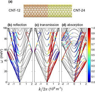
Figure 3: (a) Plot of the armchair junction between two isotopically different carbon nanotubes (CNT’s). The left CNT (‘CNT-12’) is constructed from ¹²C atoms while the right CNT (‘CNT-24’) has ²⁴C atoms. Phonon momentum and polarization-resolved plot of (b) left-lead reflection coefficients, (c) left-lead transmission coefficients, and (d) right-lead absorption coefficients for phonon transmission from CNT-12 to CNT-24.

III.3 Transition probabilities of scattering processes

In our analysis of the absorption spectrum in Fig. 3(d), we find that energy is preferentially transmitted to some phonon subbands, suggesting that transitions between phonon channels associated with certain subbands are dominant. To elucidate the role of the subbands in phonon scattering, we use our method to determine and analyze the transition probabilities between different bulk phonon channels. We analyze two sets of scattering processes, with the first corresponding to an incoming phonon channel at $k_{1}$ in the left lead (CNT-12) and the second to an incoming phonon channel at $\bar{k}_{3}$ in the right lead (CNT-24), at $\omega=39.5$ meV. Here and in our subsequent discussion of the scattering simulation results, to represent a phonon wave vector of equal magnitude but directionally opposite to $k_{i}$, we write a bar over the latter, i.e. $\bar{k}_{i}=-k_{i}$; the corresponding integer index for $\bar{k}_{i}$ is written as $\bar{i}$. The transition probabilities $P(k\rightarrow k^{\prime})$ for all available incoming and outgoing phonon channels are computed from the square of the scattering amplitudes determined from the matrix elements of $\bar{\boldsymbol{t}}_{\text{RL}}$, $\bar{\boldsymbol{t}}_{\text{LR}}$, $\bar{\boldsymbol{r}}_{\text{LL}}$ and $\bar{\boldsymbol{r}}_{\text{RR}}$.

III.3.1 Incoming phonon channel at $k_{1}$ in CNT-12 

Figures 4(a) and 4(b) show the distribution of outgoing (reflected and transmitted) phonon channels in CNT-12 [Fig. 4(a)] and CNT-24 [Fig. 4(b)] as well as the incoming phonon channel with the wave vector $k_{1}$ in CNT-12 superimposed on the phonon dispersion spectrum of CNT-12 and CNT-24. The transition probabilities between the incoming phonon channel at $k_{1}$ and its main outgoing phonon channels at $\bar{k}_{1}$, $k_{2}$ and $k_{3}$, which are all doubly degenerate, are calculated from the matrix elements of $\bar{\boldsymbol{r}}_{\text{LL}}$ and $\bar{\boldsymbol{t}}_{\text{RL}}$ and indicated in Figs. 4(a) and (b). The dominant transition probabilities [$P(k_{1}\rightarrow\bar{k}_{1})$, $P(k_{1}\rightarrow k_{2})$ and $P(k_{1}\rightarrow k_{3})$] add up to nearly unity once the two-fold degeneracy of the final phonon states is taken into account.

We find that the transmission of the incoming phonon mode at $k_{1}$, which has a transmission coefficient of $\Xi_{\text{L},1}=0.642$, is dominated by forward scattering transitions ($k_{1}\rightarrow k_{3}$) to the outgoing phonon channels at $k_{3}$, with the transition probability given by $P(k_{1}\rightarrow k_{3})=0.307$ or nearly half of the transmission coefficient, because the phonon subbands for $k_{3}$ are the CNT-24 image of the phonon subbands for $k_{1}$ as shown in Figs. 4(a) and (b), indicating that angular symmetry and polarization considerations play an important role in forward scattering. The phonon reflection processes is dominated by backward scattering to the phonon channels at $\bar{k}_{1}$ and $k_{2}$. Unusually, the $k_{1}\rightarrow\bar{k}_{1}$ transition, which corresponds to an intra-subband process, has a slightly lower probability than the $k_{1}\rightarrow k_{2}$ transition, an inter-subband process, suggesting that transitions between these two phonon subbands, indicated by bold dashed and dotted lines in panels (a) and (b), are favored in backward scattering.

III.3.2 Incoming phonon channel at $\bar{k}_{3}$ in CNT-24

Given the dominant transition between $k_{1}$ in CNT-12 and $k_{3}$ in CNT-24, it would be interesting to study the scattering processes associated with the incoming phonon channel at $\bar{k}_{3}$ in CNT-24. As before, the transition probabilities are computed from the matrix elements of $\bar{\boldsymbol{r}}_{\text{RR}}$ and $\bar{\boldsymbol{t}}_{\text{LR}}$, and shown in Figs. 4(c) and (d). We find that the transmission of the mode at $\bar{k}_{3}$, which has a transmission coefficient of $\Xi_{\text{R},\bar{3}}=0.651$, is dominated by the $\bar{k}_{3}\rightarrow\bar{k}_{1}$ process which has the transition probability of $P(\bar{k}_{3}\rightarrow\bar{k}_{1})=0.307$, numerically equal to $P(k_{1}\rightarrow k_{3})$ as expected, because the $\bar{k}_{3}\rightarrow\bar{k}_{1}$ transition is the time reversal of the $k_{1}\rightarrow k_{3}$ transition in Figs. 4(a) and (b). Also, the main reflected outgoing phonon channels in CNT-24 are at $k_{3}$ and $k_{4}$. Like in the previous simulation, the $\bar{k}_{3}\rightarrow k_{4}$ transition, an inter-subband process, plays a greater role in phonon reflection than the $\bar{k}_{3}\rightarrow k_{3}$ transition, an intra-subband process, but also to a substantially greater extent since $P(\bar{k}_{3}\rightarrow k_{4})\gg P(\bar{k}_{3}\rightarrow k_{3})$, highlighting the role of polarization in phonon scattering. The $\bar{k}_{3}\rightarrow k_{4}$ inter-subband transition is favored because the subband for $k_{4}$ is the CNT-24 image of the subband for $k_{2}$ in Fig. 4(a).

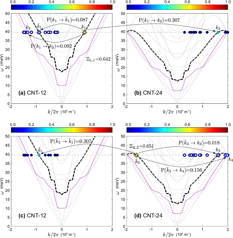
Figure 4: Plot of leftward-going phonon channels (hollow circles) in (a) CNT-12 and rightward-going phonon channels (solid circles) in (b) CNT-24 for the incoming phonon channel (square symbol) at $\omega=39.5$ meV and $k_{1}=5.65\times 10^{9}$ m^-1 in CNT-12, superimposed on the phonon dispersion curves of CNT-12 and CNT-24. The transition probability for each outgoing phonon channel from the incoming phonon at $k_{1}$ is between 0 and 1, and indicated in color. The dominant scattering processes, corresponding to (i) the $k_{1}\rightarrow\bar{k}_{1}$ intra-subband reflection, (ii) the $k_{1}\rightarrow k_{2}$ inter-subband reflection, and (iii) the $k_{1}\rightarrow k_{3}$ transmission, are drawn with dotted arrows with the transition probabilities explicitly given. The outgoing phonon channels in (c) CNT-12 and (d) CNT-24 for the incoming phonon channel at $\omega=39.5$ meV and $\bar{k}_{3}$ in CNT-24 are also shown. The main outgoing phonon channels for the incoming phonon at $\bar{k}_{3}$ are at $\bar{k}_{1}$, $k_{3}$ and $k_{4}$ and also indicated by dotted arrows with the transition probabilities given. To guide the eye, the subbands for $k_{1}$, $\bar{k}_{1}$, $k_{3}$ and $\bar{k}_{3}$ are indicated in bold dashed lines while the subbands for $k_{2}$ and $k_{4}$ are indicated in bold magenta dotted lines.

IV Example with zigzag and armchair graphene edge

To illustrate the utility of our method for studying boundary scattering, we apply the $S$-matrix method to investigate the effects of edge orientation and structure on phonon scattering in graphene. Unlike the previous example of the CNT junction, there is no phonon transmission as we are dealing with pure phonon reflection in which every incoming phonon is backscattered elastically into a range of outgoing phonon channels. The phonon scattering specularity, important for understanding phonon transport in graphene nanoribbons,(Hu et al., 2009; Bae et al., 2013; Majee and Aksamija, 2016) can be obtained from the distribution of the transition probabilities.

In addition, because the system is a two-dimensional one in which we partition the lattice into unit cells larger than the usual primitive unit cell, two additional intermediate procedures are needed in the application of our $S$-matrix method to graphene. The first procedure deals with the periodic boundary conditions in the transverse direction which affect the structure of the matrices $\boldsymbol{H}_{\text{L}}^{00}$ and $\boldsymbol{H}_{\text{L}}^{01}$ associated with the bulk lead and permit us to decompose them into their Fourier-component submatrices, facilitating the efficient computation of the surface and bulk Green’s functions. This Fourier decomposition requires us to partition the rectangular slices in Fig. 1 into unit cells in the transverse direction [Fig. 5(a)] and index the incoming and outgoing phonon channels with wave vectors associated with phonon modes in the ‘folded’ Brillouin zone [Fig. 5(b)] which follows from the transverse partitioning of the rectangular slices in Fig. 1. The second procedure deals with the mapping of the phonon modes in the ‘folded’ Brillouin zone to the bulk phonon eigenmodes in the standard ‘unfolded’ Brillouin zone associated with the symmetry of the primitive unit cell in graphene. Although this step is not strictly necessary, the use of the zone-unfolding technique, as described by Boykin and Klimeck, (Boykin and Klimeck, 2005; Boykin et al., 2009) improves the clarity of the scattering results by presenting their analysis in more familiar terms.

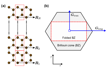
Figure 5: (a) Schematic of the bulk graphene slice (bounded by dotted lines) for the armchair edge scattering simulation. Each slice is partitioned in the transverse ($y$) direction into 4-atom unit cells. (b) The 4-atom unit cell is twice as large as the 2-atom primitive unit cell, resulting in a smaller folded Brillouin zone (bounded by dashed lines) with half the area of the standard Brillouin zone (bounded by solid lines). The longitudinal and transverse reciprocal lattice vectors for the folded BZ are given by $\boldsymbol{G}_{\text{long}}$ and $\boldsymbol{G}_{\text{tran}}$, respectively.

IV.1 Calculation details

Like in the previous example, we construct the bulk graphene monolayer and optimize its structure in GULP (Gale and Rohl, 2003) using the same Tersoff potential parameters. (Lindsay and Broido, 2010). We assume that the graphene edge is terminated on the right and its bulk extends infinitely to the left. Thus, unlike the schematic shown in Fig. (1), we need only to consider the force-constant matrices $\boldsymbol{H}_{\text{L}}^{00}$ and $\boldsymbol{H}_{\text{L}}^{01}$ to describe the left bulk and $\boldsymbol{H}_{\text{C}}$ and $\boldsymbol{H}_{\text{CL}}$ to describe the graphene edge and its coupling to the left bulk. The force-constant matrices $\boldsymbol{H}_{\text{R}}^{00}$, $\boldsymbol{H}_{\text{R}}^{01}$ and $\boldsymbol{H}_{\text{CR}}$ in Eq. (1) are not needed in this study and their matrix elements are set to zero.

The force-constant matrices for the bulk slices ($\boldsymbol{H}_{\text{L}}^{00}$ and $\boldsymbol{H}_{\text{L}}^{01}$) are computed in GULP. For the armchair and zigzag edge structures, the slices in the leads each have $4N$ atoms. We take advantage of the periodicity in the transverse direction to partition the slice into $N$ 4-atom unit cells, as shown in Fig. 5(a), at the real lattice points $\boldsymbol{R}_{1},\ldots,\boldsymbol{R}_{N}$ where $\boldsymbol{R}_{p}=(p-1)\boldsymbol{T}$ and $\boldsymbol{T}$ is the lattice vector characterizing the transverse periodicity. The $12\times 12$ force-constant submatrix corresponding to the coupling between the unit cells at $\boldsymbol{R}_{p}$ and $\boldsymbol{R}_{q}$ within the same slice is denoted as $\mathbf{H}_{\text{L}}^{00}(\boldsymbol{R}_{p},\boldsymbol{R}_{q})$ while the $12\times 12$ force-constant submatrix corresponding to the coupling between the unit cell at $\boldsymbol{R}_{p}$ in the slice and the unit cell at $\boldsymbol{R}_{q}$ in the slice on the right (left) is denoted by $\mathbf{H}_{\text{L}}^{01}(\boldsymbol{R}_{p},\boldsymbol{R}_{q})$ [$\mathbf{H}_{\text{L}}^{10}(\boldsymbol{R}_{p},\boldsymbol{R}_{q})$].

The transverse translational symmetry implies that the force-constant submatrices depend only on the relative displacement between the unit cells in the transverse direction, i.e.

$$\mathbf{H}_{\text{L}}^{lm}(\boldsymbol{R}_{p},\boldsymbol{R}_{q})=\mathbf{H}_{\text{L}}^{lm}(\boldsymbol{R}_{p}-\boldsymbol{R}_{q})$$ (34)

for $l=0,1$ and $m=(l-1)\mod 2$. For a slice with $N$ transverse unit cells, the submatrices make up the $12N\times 12N$ matrix associated with the entire slice,

$$\boldsymbol{H}_{\text{L}}^{lm}=\left(\begin{array}[]{cccc}\mathbf{H}_{\text{L}}^{lm}(\boldsymbol{R}_{1},\boldsymbol{R}_{1})&\mathbf{H}_{\text{L}}^{lm}(\boldsymbol{R}_{1},\boldsymbol{R}_{2})&\cdots&\mathbf{H}_{\text{L}}^{lm}(\boldsymbol{R}_{1},\boldsymbol{R}_{N})\\ \mathbf{H}_{\text{L}}^{lm}(\boldsymbol{R}_{2},\boldsymbol{R}_{1})&\mathbf{H}_{\text{L}}^{lm}(\boldsymbol{R}_{2},\boldsymbol{R}_{2})&\cdots&\mathbf{H}_{\text{L}}^{lm}(\boldsymbol{R}_{2},\boldsymbol{R}_{N})\\ \vdots&\vdots&\ddots&\vdots\\ \mathbf{H}_{\text{L}}^{lm}(\boldsymbol{R}_{N},\boldsymbol{R}_{1})&\mathbf{H}_{\text{L}}^{lm}(\boldsymbol{R}_{N},\boldsymbol{R}_{2})&\cdots&\mathbf{H}_{\text{L}}^{lm}(\boldsymbol{R}_{N},\boldsymbol{R}_{N})\end{array}\right)\ .$$ (39)

It follows from Eq. (39) that $\mathbf{H}_{\text{L}}^{ml}(\boldsymbol{R}_{q},\boldsymbol{R}_{p})=\mathbf{H}_{\text{L}}^{lm}(\boldsymbol{R}_{p},\boldsymbol{R}_{q})^{\dagger}$. In addition, Eq. (34) and the transverse periodic boundary conditions imply that we can write Eq. (39) as

$$\boldsymbol{H}_{\text{L}}^{lm}=\left(\begin{array}[]{cccc}\mathbf{H}_{\text{L}}^{lm}(0)&\mathbf{H}_{\text{L}}^{lm}(-\boldsymbol{T})&\cdots&\mathbf{H}_{\text{L}}^{lm}(-(N-1)\boldsymbol{T})\\ \mathbf{H}_{\text{L}}^{lm}(-(N-1)\boldsymbol{T})&\mathbf{H}_{\text{L}}^{lm}(0)&\cdots&\mathbf{H}_{\text{L}}^{lm}(-(N-2)\boldsymbol{T})\\ \vdots&\vdots&\ddots&\vdots\\ \mathbf{H}_{\text{L}}^{lm}(-\boldsymbol{T})&\mathbf{H}_{\text{L}}^{lm}(-2\boldsymbol{T})&\cdots&\mathbf{H}_{\text{L}}^{lm}(0)\end{array}\right)\ ,$$ (40)

which has the form of a block-circulant matrix. (De Mazancourt and Gerlic, 1983)

IV.1.1 Working with transverse Fourier components

Although it seems natural to use Eq. (4b) directly to determine the surface Green’s function, it is numerically more efficient to exploit the block-circulant matrix structure of Eq. (40) by employing a discrete Fourier-transform approach like in Ref. (De Mazancourt and Gerlic, 1983) which also yields a set of indices $\boldsymbol{Q}_{n}$, where $n=0,\ldots,N-1$, associated with the periodicity in the transverse direction. The matrix $\boldsymbol{H}_{\text{L}}^{lm}$ in Eq. (40) can be transformed into the block-diagonal form $\tilde{\boldsymbol{H}}_{\text{L}}^{lm}$, via the expression

$$\boldsymbol{H}_{\text{L}}^{lm}=\boldsymbol{P}\tilde{\boldsymbol{H}}_{\text{L}}^{lm}\boldsymbol{P}^{-1}$$ (41)

where

$$\boldsymbol{P}=\frac{1}{\sqrt{N}}\left(\begin{array}[]{cccc}\tilde{\mathbf{I}}_{\text{L}}e^{i\boldsymbol{Q}_{1}\cdot\boldsymbol{R}_{1}}&\tilde{\mathbf{I}}_{\text{L}}e^{i\boldsymbol{Q}_{2}\cdot\boldsymbol{R}_{1}}&\cdots&\tilde{\mathbf{I}}_{\text{L}}e^{i\boldsymbol{Q}_{N}\cdot\boldsymbol{R}_{1}}\\ \tilde{\mathbf{I}}_{\text{L}}e^{i\boldsymbol{Q}_{1}\cdot\boldsymbol{R}_{2}}&\tilde{\mathbf{I}}_{\text{L}}e^{i\boldsymbol{Q}_{2}\cdot\boldsymbol{R}_{2}}&\cdots&\tilde{\mathbf{I}}_{\text{L}}e^{i\boldsymbol{Q}_{N}\cdot\boldsymbol{R}_{2}}\\ \vdots&\vdots&\ddots&\vdots\\ \tilde{\mathbf{I}}_{\text{L}}e^{i\boldsymbol{Q}_{1}\cdot\boldsymbol{R}_{N}}&\tilde{\mathbf{I}}_{\text{L}}e^{i\boldsymbol{Q}_{2}\cdot\boldsymbol{R}_{N}}&\cdots&\tilde{\mathbf{I}}_{\text{L}}e^{i\boldsymbol{Q}_{N}\cdot\boldsymbol{R}_{N}}\end{array}\right)$$ (42)

is the special unitary matrix used for the basis transformation, $\tilde{\mathbf{I}}_{\text{L}}$ is the $12\times 12$ identity submatrix, and $\tilde{\boldsymbol{H}}_{\text{L}}^{lm}$ is

$$\tilde{\boldsymbol{H}}_{\text{L}}^{lm}=\left(\begin{array}[]{cccc}\tilde{\mathbf{H}}_{\text{L}}^{lm}(\boldsymbol{Q}_{1})\\ &\tilde{\mathbf{H}}_{\text{L}}^{lm}(\boldsymbol{Q}_{2})\\ &&\ddots\\ &&&\tilde{\mathbf{H}}_{\text{L}}^{lm}(\boldsymbol{Q}_{N})\end{array}\right)\ .$$ (43)

Each diagonal submatrix in Eq. (43) is the discrete Fourier transform of $\mathbf{H}_{\text{L}}^{lm}(\boldsymbol{R}_{p},\boldsymbol{R}_{q})$, i.e.

$$\tilde{\mathbf{H}}_{\text{L}}^{lm}(\boldsymbol{Q}_{n})=\sum_{q=0}^{N-1}\mathbf{H}_{\text{L}}^{lm}(\boldsymbol{R}_{p},\boldsymbol{R}_{p+q})e^{-i\boldsymbol{Q}_{n}\cdot(\boldsymbol{R}_{p}-\boldsymbol{R}_{p+q})}$$ (44)

where $l=0,1$ and $m=(l-1)\mod 2$, and represents a transverse Fourier component corresponding to the transverse wave vector $\boldsymbol{Q}_{n}=\frac{n}{N}\boldsymbol{G}_{\text{tran}}$, where $n=0,\ldots,N-1$, and $\boldsymbol{G}_{\text{tran}}$ is the transverse reciprocal lattice vector satisfying $\boldsymbol{G}_{\text{tran}}\cdot\boldsymbol{T}=2\pi$. It can also be shown that $\tilde{\mathbf{H}}_{\text{L}}^{ml}(\boldsymbol{Q}_{n})=[\tilde{\mathbf{H}}_{\text{L}}^{lm}(\boldsymbol{Q}_{n})]^{\dagger}$.

The block-diagonal form of Eq. (43) allows us to treat each Fourier component as an effectively independent subsystem and determine piecewise the essential matrix variables such as the surface Green’s functions from the force-constant submatrices $\tilde{\mathbf{H}}_{\text{L}}^{00}(\boldsymbol{Q}_{n})$ and $\tilde{\mathbf{H}}_{\text{L}}^{01}(\boldsymbol{Q}_{n})$, using the methodology described in Sec. II. In the following discussions, we use the $\boldsymbol{B}_{\text{L},\pm}^{\text{adv/ret}}$ as a shorthand notation to refer to the four related matrices $\boldsymbol{B}_{\text{L},+}^{\text{ret}}$, $\boldsymbol{B}_{\text{L},-}^{\text{ret}}$, $\boldsymbol{B}_{\text{L},+}^{\text{adv}}$ and $\boldsymbol{B}_{\text{L},-}^{\text{adv}}$ where $\boldsymbol{B}$ is any matrix function (e.g. the surface Green’s function $\boldsymbol{g}$).

In the same manner, the surface Green’s function can be block-diagonalized with the same $\boldsymbol{P}$ in Eq. (41), i.e.,

$$\boldsymbol{g}_{\text{L},\pm}^{\text{adv/ret}}=\boldsymbol{P}\tilde{\boldsymbol{g}}_{\text{L},\pm}^{\text{adv/ret}}\boldsymbol{P}^{-1}$$ (45)

where $\tilde{\boldsymbol{g}}_{\text{L},\pm}^{\text{adv/ret}}$ is a block-diagonal matrix like $\tilde{\boldsymbol{H}}_{\text{L}}^{lm}$ in Eq. (43) and has the block-diagonal $12\times 12$ submatrices $\tilde{\mathbf{g}}_{\text{L},\pm}^{\text{adv/ret}}(\boldsymbol{Q}_{n})$ for $n=1,\ldots,N$, with

$$\tilde{\mathbf{g}}_{\text{L},-}^{\text{ret}}(\boldsymbol{Q}_{n})=[(\omega^{2}+i\eta)\tilde{\mathbf{I}}_{\text{L}}-\mathbf{\tilde{H}}_{\text{L}}^{00}(\boldsymbol{Q}_{n})-\mathbf{\tilde{H}}_{\text{L}}^{10}(\boldsymbol{Q}_{n})\tilde{\mathbf{g}}_{\text{L},-}^{\text{ret}}(\boldsymbol{Q}_{n})\mathbf{\tilde{H}}_{\text{L}}^{01}(\boldsymbol{Q}_{n})]^{-1}$$ (46a)

$$\tilde{\mathbf{g}}_{\text{L},+}^{\text{ret}}(\boldsymbol{Q}_{n})=[(\omega^{2}+i\eta)\tilde{\mathbf{I}}_{\text{L}}-\mathbf{\tilde{H}}_{\text{L}}^{00}(\boldsymbol{Q}_{n})-\mathbf{\tilde{H}}_{\text{L}}^{01}(\boldsymbol{Q}_{n})\tilde{\mathbf{g}}_{\text{L},+}^{\text{ret}}(\boldsymbol{Q}_{n})\mathbf{\tilde{H}}_{\text{L}}^{10}(\boldsymbol{Q}_{n})]^{-1}$$ (46b)

like in Eq. (4b) and $\tilde{\mathbf{g}}_{\text{L},\pm}^{\text{adv}}(\boldsymbol{Q}_{n})=\tilde{\mathbf{g}}_{\text{L},\pm}^{\text{ret}}(\boldsymbol{Q}_{n})^{\dagger}$.

Similarly, we have the block-diagonal Bloch matrices $\tilde{\boldsymbol{F}}_{\text{L},\pm}^{\text{adv/ret}}$ with the diagonal submatrices $\tilde{\mathbf{F}}_{\text{L},\pm}^{\text{adv/ret}}(\boldsymbol{Q}_{n})$ given by $\tilde{\mathbf{F}}_{\text{L},+}^{\text{adv/ret}}(\boldsymbol{Q}_{n})=\tilde{\mathbf{g}}_{\text{L},+}^{\text{adv/ret}}(\boldsymbol{Q}_{n})\mathbf{\tilde{H}}_{\text{L}}^{10}(\boldsymbol{Q}_{n})$ and $\tilde{\mathbf{F}}_{\text{L},-}^{\text{adv/ret}}(\boldsymbol{Q}_{n})=\tilde{\mathbf{g}}_{\text{L},-}^{\text{adv/ret}}(\boldsymbol{Q}_{n})\mathbf{\tilde{H}}_{\text{L}}^{01}(\boldsymbol{Q}_{n})$ from Eq. (7b). The bulk eigenmode submatrices $\tilde{\mathbf{U}}_{\text{L},\pm}^{\text{adv/ret}}(\boldsymbol{Q}_{n})$ are determined from Eq. (8b), i.e., $\tilde{\mathbf{F}}_{\text{L},+}^{\text{adv/ret}}(\boldsymbol{Q}_{n})\tilde{\mathbf{U}}_{\text{L},+}^{\text{adv/ret}}(\boldsymbol{Q}_{n})=\tilde{\mathbf{U}}_{\text{L},+}^{\text{adv/ret}}(\boldsymbol{Q}_{n})\tilde{\boldsymbol{\Lambda}}_{\text{L},+}^{\text{adv/ret}}(\boldsymbol{Q}_{n})$ and $\tilde{\mathbf{F}}_{\text{L},-}^{\text{adv/ret}}(\boldsymbol{Q}_{n})^{-1}\tilde{\mathbf{U}}_{\text{L},-}^{\text{adv/ret}}(\boldsymbol{Q}_{n})=\tilde{\mathbf{U}}_{\text{L},-}^{\text{adv/ret}}(\boldsymbol{Q}_{n})\tilde{\boldsymbol{\Lambda}}_{\text{L},-}^{\text{adv/ret}}(\boldsymbol{Q}_{n})^{-1}$. As in Eq. (8b), the matrices $\tilde{\boldsymbol{\Lambda}}_{\text{L},\pm}^{\text{adv/ret}}(\boldsymbol{Q}_{n})$ have only diagonal elements containing the eigenvalues of $\tilde{\mathbf{F}}_{\text{L},\pm}^{\text{adv/ret}}$ and make up the block-diagonal submatrices in

$$\tilde{\boldsymbol{\Lambda}}_{\text{L},\pm}^{\text{adv/ret}}=\left(\begin{array}[]{cccc}\tilde{\boldsymbol{\Lambda}}_{\text{L},\pm}^{\text{adv/ret}}(\boldsymbol{Q}_{1})\\ &\tilde{\boldsymbol{\Lambda}}_{\text{L},\pm}^{\text{adv/ret}}(\boldsymbol{Q}_{2})\\ &&\ddots\\ &&&\tilde{\boldsymbol{\Lambda}}_{\text{L},\pm}^{\text{adv/ret}}(\boldsymbol{Q}_{N})\end{array}\right)$$ (47)

which is a purely diagonal $12N\times 12N$ matrix. The Bloch eigenmode matrices have the form

$$\tilde{\mathbf{U}}_{\text{L},\pm}^{\text{adv/ret}}(\boldsymbol{Q}_{n})=\left(\begin{array}[]{ccc}\tilde{\mathbf{u}}_{\text{L},\pm}^{\text{adv/ret}}(\boldsymbol{Q}_{n},k_{n,1}),&\ldots,&\tilde{\mathbf{u}}_{\text{L},\pm}^{\text{adv/ret}}(\boldsymbol{Q}_{n},k_{n,12})\end{array}\right)$$ (48)

where $\tilde{\mathbf{u}}_{\text{L},\pm}^{\text{adv/ret}}(\boldsymbol{Q}_{n},k_{n,m})$ is the $12\times 1$ column eigenvector for the transverse wave vector $\boldsymbol{Q}_{n}$ and the longitudinal wave vector $k_{n,m}$ for $m=1,\ldots,12$. The corresponding eigenvelocity submatrices $\tilde{\mathbf{V}}_{\text{L},\pm}^{\text{adv/ret}}(\boldsymbol{Q}_{n})$ can be found using Eqs. (9) and (10), and have the form

$$\tilde{\mathbf{V}}_{\text{L},\pm}^{\text{adv/ret}}(\boldsymbol{Q}_{n})=\left(\begin{array}[]{ccc}v_{\text{L},\pm}^{\text{adv/ret}}(\boldsymbol{Q}_{n},k_{n,1})&\cdots&0\\ \vdots&\ddots&\vdots\\ 0&\cdots&v_{\text{L},\pm}^{\text{adv/ret}}(\boldsymbol{Q}_{n},k_{n,12})\end{array}\right)$$

where is $v_{\text{L},\pm}^{\text{adv/ret}}(\boldsymbol{Q}_{n},k_{n,m})$ is the corresponding longitudinal group velocity for the eigenmode $\tilde{\mathbf{u}}_{\text{L},\pm}^{\text{adv/ret}}(\boldsymbol{Q}_{n},k_{n,m})$.

IV.1.2 Real space matrix variables

To recover the real-space surface Green’s function matrix $\boldsymbol{g}_{\text{L},\pm}^{\text{adv/ret}}$, we apply the transformation $\boldsymbol{g}_{\text{L},\pm}^{\text{adv/ret}}=\boldsymbol{P}\tilde{\boldsymbol{g}}_{\text{L},\pm}^{\text{adv/ret}}\boldsymbol{P}^{-1}$ like in Eq. (45) and obtain

$$\boldsymbol{g}_{\text{L},\pm}^{\text{adv/ret}}=\left(\begin{array}[]{cccc}\mathbf{g}_{\text{L},\pm}^{\text{adv/ret}}(\boldsymbol{R}_{1},\boldsymbol{R}_{1})&\mathbf{g}_{\text{L},\pm}^{\text{adv/ret}}(\boldsymbol{R}_{1},\boldsymbol{R}_{2})&\cdots&\mathbf{g}_{\text{L},\pm}^{\text{adv/ret}}(\boldsymbol{R}_{1},\boldsymbol{R}_{N})\\ \mathbf{g}_{\text{L},\pm}^{\text{adv/ret}}(\boldsymbol{R}_{2},\boldsymbol{R}_{1})&\mathbf{g}_{\text{L},\pm}^{\text{adv/ret}}(\boldsymbol{R}_{2},\boldsymbol{R}_{2})&\cdots&\mathbf{g}_{\text{L},\pm}^{\text{adv/ret}}(\boldsymbol{R}_{2},\boldsymbol{R}_{N})\\ \vdots&\vdots&\ddots&\vdots\\ \mathbf{g}_{\text{L},\pm}^{\text{adv/ret}}(\boldsymbol{R}_{N},\boldsymbol{R}_{1})&\mathbf{g}_{\text{L},\pm}^{\text{adv/ret}}(\boldsymbol{R}_{N},\boldsymbol{R}_{2})&\cdots&\mathbf{g}_{\text{L},\pm}^{\text{adv/ret}}(\boldsymbol{R}_{N},\boldsymbol{R}_{N})\end{array}\right)\ .$$ (49)

Similarly, the real-space Bloch matrix from Eq. (7b) can be obtained via the expression $\boldsymbol{F}_{\text{L}}^{\text{adv/ret}}(\pm)=\boldsymbol{P}\tilde{\boldsymbol{F}}_{\text{L},\pm}^{\text{adv/ret}}\boldsymbol{P}^{-1}$. Given that the real-space Bloch matrix must satisfy the conditions

$$\boldsymbol{F}_{\text{L}}^{\text{adv/ret}}(\pm)^{\pm 1}\boldsymbol{U}_{\text{L}}^{\text{adv/ret}}(\pm)=\boldsymbol{U}_{\text{L}}^{\text{adv/ret}}(\pm)\boldsymbol{\Lambda}_{\text{L}}^{\text{adv/ret}}(\pm)^{\pm}$$ (50)

where $\boldsymbol{\Lambda}_{\text{L}}^{\text{adv/ret}}(\pm)$ is also a purely diagonal matrix like $\tilde{\boldsymbol{\Lambda}}_{\text{L},\pm}^{\text{adv/ret}}$ with the eigenvalues of $\boldsymbol{F}_{\text{L}}^{\text{adv/ret}}(\pm)$ along its diagonal. Equation (50) implies that $\boldsymbol{\Lambda}_{\text{L}}^{\text{adv/ret}}(\pm)=\tilde{\boldsymbol{\Lambda}}_{\text{L},\pm}^{\text{adv/ret}}$ and we can write the real-space bulk eigenmode matrix as

$$\boldsymbol{U}_{\text{L}}^{\text{adv/ret}}(\pm)=\boldsymbol{P}\tilde{\boldsymbol{U}}_{\text{L},\pm}^{\text{adv/ret}}\ ,$$ (51)

giving us

$$\boldsymbol{U}_{\text{L}}^{\text{adv/ret}}(\pm) =\frac{1}{\sqrt{N}}\left(\begin{array}[]{cccc}\tilde{\mathbf{U}}_{\text{L},\pm}^{\text{adv/ret}}(\boldsymbol{Q}_{1})e^{i\boldsymbol{Q}_{1}\cdot\boldsymbol{R}_{1}}&\tilde{\mathbf{U}}_{\text{L},\pm}^{\text{adv/ret}}(\boldsymbol{Q}_{2})e^{i\boldsymbol{Q}_{2}\cdot\boldsymbol{R}_{1}}&\cdots&\tilde{\mathbf{U}}_{\text{L},\pm}^{\text{adv/ret}}(\boldsymbol{Q}_{N})e^{i\boldsymbol{Q}_{N}\cdot\boldsymbol{R}_{1}}\\ \tilde{\mathbf{U}}_{\text{L},\pm}^{\text{adv/ret}}(\boldsymbol{Q}_{1})e^{i\boldsymbol{Q}_{1}\cdot\boldsymbol{R}_{2}}&\tilde{\mathbf{U}}_{\text{L},\pm}^{\text{adv/ret}}(\boldsymbol{Q}_{2})e^{i\boldsymbol{Q}_{2}\cdot\boldsymbol{R}_{2}}&\cdots&\tilde{\mathbf{U}}_{\text{L},\pm}^{\text{adv/ret}}(\boldsymbol{Q}_{N})e^{i\boldsymbol{Q}_{N}\cdot\boldsymbol{R}_{2}}\\ \vdots&\vdots&\ddots&\vdots\\ \tilde{\mathbf{U}}_{\text{L},\pm}^{\text{adv/ret}}(\boldsymbol{Q}_{1})e^{i\boldsymbol{Q}_{1}\cdot\boldsymbol{R}_{N}}&\tilde{\mathbf{U}}_{\text{L},\pm}^{\text{adv/ret}}(\boldsymbol{Q}_{2})e^{i\boldsymbol{Q}_{2}\cdot\boldsymbol{R}_{N}}&\cdots&\tilde{\mathbf{U}}_{\text{L},\pm}^{\text{adv/ret}}(\boldsymbol{Q}_{N})e^{i\boldsymbol{Q}_{N}\cdot\boldsymbol{R}_{N}}\end{array}\right)$$ (56)

$$=\left(\begin{array}[]{c}\mathbf{u}_{\text{L},\pm}^{\text{adv/ret}}(\boldsymbol{Q}_{1},k_{1,1}),\ldots,\mathbf{\mathbf{u}}_{\text{L},\pm}^{\text{adv/ret}}(\boldsymbol{Q}_{1},k_{1,12}),\ldots,\mathbf{\mathbf{u}}_{\text{L},\pm}^{\text{adv/ret}}(\boldsymbol{Q}_{N},k_{N,1}),\ldots,\mathbf{u}_{\text{L},\pm}^{\text{adv/ret}}(\boldsymbol{Q}_{N},k_{N,12})\end{array}\right)$$ (58)

where the right-hand side of Eq. (56) is a $12N\times 12N$ matrix with each column vector corresponding to an extended or evanescent bulk eigenmode and represented by $\mathbf{u}_{\text{L},\pm}^{\text{adv/ret}}(\boldsymbol{Q}_{n},k_{n,m})$, where $n=1,\ldots,N$ and $m=1,\ldots,12$. Hence, we have a total of $12N$ eigenmodes, associated with each is a real or complex longitudinal wave vector. For each transverse wave vector $\boldsymbol{Q}_{n}$, we have $12$ longitudinal wave vectors which we enumerate as $k_{n,1}$ to $k_{n,12}$. It also follows from Eqs. (50) and (51) that the real-space velocity matrix is $\boldsymbol{V}_{\text{L}}^{\text{adv/ret}}(\pm)=\tilde{\boldsymbol{V}}_{\text{L},\pm}^{\text{adv/ret}}$.

Given the real-space surface Green’s functions in Eq. (49), we can compute the effective harmonic matrix in Eq. (3) and the corresponding Green’s function $\boldsymbol{G}_{\text{L}}^{\text{ret}}$ from Eq. (5). Using $\boldsymbol{V}_{\text{L}}^{\text{ret/adv}}(-)$ and $\boldsymbol{U}_{\text{L}}^{\text{ret/adv}}(-)$ from Eq. (56), we compute $\bar{\boldsymbol{r}}_{\text{LL}}$ from Eq. (20) which gives us the transition amplitudes between the incoming and outgoing phonon channels.

IV.1.3 Brillouin zone unfolding

In our transverse partitioning scheme, we can associate with each phonon channel in Eq. (56) a transverse wave vector $\boldsymbol{Q}_{n}$ and its longitudinal wave vector $k_{n,m}$. The vector sum of these two wave vectors ($\boldsymbol{k}=\boldsymbol{Q}_{n}+k_{n,m}\hat{\boldsymbol{x}}$ where the longitudinal direction is in the $x$ direction) yields the locus of the mode ($\boldsymbol{k}$) within the ‘folded’ Brillouin zone (BZ) as shown in Fig. 5(b). This folded BZ is a consequence of the 4-atom unit supercell used in our $S$-matrix method, which requires the partitioning of the atomic degrees of freedom into rectangular slices, and thus has half the reciprocal space area of the primitive BZ but contains 12 phonon branches compared to 6 phonon branches in the primitive BZ.

To make sense of our analysis of the transmission coefficients and individual transition amplitudes, it is necessary to map the scattering channels to the phonon modes in the bulk graphene lattice. This is done by ‘unfolding’ the 12 phonon branches within the folded BZ to obtain 6 phonon branches within the larger primitive BZ using the zone-unfolding technique of Boykin and Klimeck. (Boykin and Klimeck, 2005; Boykin et al., 2009) Given our choice of the 4-atom unit supercell, each phonon mode ($\boldsymbol{k}$) in the folded BZ has two possible image points ($\boldsymbol{k}^{\prime}$) in the primitive BZ, with one of them satisfying $\boldsymbol{k}^{\prime}=\boldsymbol{k}$ and the other shifted by an integer multiple of $\boldsymbol{G}_{\text{long}}$ and $\boldsymbol{G}_{\text{tran}}$, i.e. $\boldsymbol{k}^{\prime}=\boldsymbol{k}+n_{1}\boldsymbol{G}_{\text{long}}+n_{2}\boldsymbol{G}_{\text{tran}}$, where $n_{1}$ and $n_{2}$ are whole numbers that depend on $\boldsymbol{k}$. For notational brevity, we write $\boldsymbol{k}^{\prime}=\boldsymbol{k}+\boldsymbol{G}(\boldsymbol{k})$. However, only one of the two image points corresponds to the correct bulk mode, except in the special case where $\boldsymbol{Q}_{n}=-\boldsymbol{G}_{\text{tran}}/2$ and all the phonon modes are two-fold degenerate.

For completeness, we outline the application of the Boykin-Klimeck unfolding technique (Boykin and Klimeck, 2005; Boykin et al., 2009) to the graphene lattice. We write the $12\times 1$ column eigenvector $\tilde{\mathbf{u}}_{\text{L},\pm}^{\text{adv/ret}}(\boldsymbol{Q}_{n},k_{n,m})$ in Eq. (48), after dropping the superscripts and subscripts for the sake of brevity, as

$$\tilde{\mathbf{u}}(\boldsymbol{k})=\left(\begin{array}[]{c}\tilde{\boldsymbol{\beta}}_{1}(\boldsymbol{k})\\ \tilde{\boldsymbol{\beta}}_{2}(\boldsymbol{k})\end{array}\right)\ ,$$ (59)

where, for $n=1,2$, $\tilde{\boldsymbol{\beta}}_{n}(\boldsymbol{k})$ is the $6\times 1$ column vector corresponding to $n$-th 2-atom primitive unit cell of the 4-atom supercell, and $\boldsymbol{\rho}_{n}$ is its displacement vector within the supercell. From Eq. (59), we define the $12\times 1$ column vector

$$\tilde{\boldsymbol{B}}(\boldsymbol{k})=\left(\begin{array}[]{c}\tilde{\boldsymbol{\beta}}_{1}(\boldsymbol{k})e^{-i\boldsymbol{k}\cdot\boldsymbol{\rho}_{1}}\\ \tilde{\boldsymbol{\beta}}_{2}(\boldsymbol{k})e^{-i\boldsymbol{k}\cdot\boldsymbol{\rho}_{2}}\end{array}\right)$$

and the $12\times 12$ matrix

$$\boldsymbol{W}(\boldsymbol{k})=\frac{1}{\sqrt{2}}\left(\begin{array}[]{cc}\tilde{\boldsymbol{I}}&\tilde{\boldsymbol{I}}e^{i\boldsymbol{G}(\boldsymbol{k})\cdot\boldsymbol{\rho}_{1}}\\ \tilde{\boldsymbol{I}}&\tilde{\boldsymbol{I}}e^{i\boldsymbol{G}(\boldsymbol{k})\cdot\boldsymbol{\rho}_{2}}\end{array}\right)\ ,$$

where $\tilde{\boldsymbol{I}}$ is the $6\times 6$ identity matrix. The $12\times 1$ column vector $\tilde{\boldsymbol{C}}(\boldsymbol{k})$ containing the unfolded modes is given by (Boykin and Klimeck, 2005; Boykin et al., 2009)

$$\tilde{\boldsymbol{C}}(\boldsymbol{k})=\left(\begin{array}[]{c}\tilde{\mathbf{c}}_{\boldsymbol{k}}\\ \tilde{\mathbf{c}}_{\boldsymbol{k}+\boldsymbol{G}(\boldsymbol{k})}\end{array}\right)=\boldsymbol{W}(\boldsymbol{k})^{-1}\tilde{\boldsymbol{B}}(\boldsymbol{k})$$ (60)

where $\tilde{\mathbf{c}}_{\boldsymbol{k}}$ and $\tilde{\mathbf{c}}_{\boldsymbol{k}+\boldsymbol{G}(\boldsymbol{k})}$ are the $6\times 1$ column vectors corresponding to the the possible unfolded eigenmodes at $\boldsymbol{k}^{\prime}=\boldsymbol{k}$ and $\boldsymbol{k}^{\prime}=\boldsymbol{k}+\boldsymbol{G}(\boldsymbol{k})$, respectively. If the folded mode in Eq. (59) is not degenerate, then only one of the two possible unfolded eigenmodes in Eq. (60) is correct and the correct unfolded wave vector can be identified through elimination as the incorrect eigenmode is zero in all its components. Using Eq. (60) as an example, if $|\tilde{\mathbf{c}}_{\boldsymbol{k}}|=0$, then the correct unfolded wave vector is $\boldsymbol{k}^{\prime}=\boldsymbol{k}+\boldsymbol{G}(\boldsymbol{k})$ and the corresponding eigenvector is given by

$$\tilde{\mathbf{u}}(\boldsymbol{k})\rightarrow\tilde{\mathbf{u}}(\boldsymbol{k})=\frac{|\tilde{\boldsymbol{B}}(\boldsymbol{k})|}{\sqrt{2}|\tilde{\mathbf{c}}_{\boldsymbol{k}+\boldsymbol{G}(\boldsymbol{k})}|}\left(\begin{array}[]{c}\tilde{\mathbf{c}}_{\boldsymbol{k}+\boldsymbol{G}(\boldsymbol{k})}e^{i\boldsymbol{k}\cdot\boldsymbol{\rho}_{1}}\\ \tilde{\mathbf{c}}_{\boldsymbol{k}+\boldsymbol{G}(\boldsymbol{k})}e^{i\boldsymbol{k}\cdot\boldsymbol{\rho}_{2}}\end{array}\right)\ .$$

On the other hand, if the folded mode in Eq. (59) is degenerate, i.e. there are other modes that share its wave vector and frequency, then it is possible that neither $|\tilde{\mathbf{c}}_{\boldsymbol{k}}|=0$ nor $|\tilde{\mathbf{c}}_{\boldsymbol{k}+\boldsymbol{G}(\boldsymbol{k})}|=0$, and hence both $\tilde{\mathbf{c}}_{\boldsymbol{k}}$ and $\tilde{\mathbf{c}}_{\boldsymbol{k}+\boldsymbol{G}(\boldsymbol{k})}$ represent correct unfolded eigenmodes, of which we may consider $\tilde{\mathbf{u}}(\boldsymbol{k})$ in Eq. (59) as a mix. We can “unmix’ ’ the degenerate folded eigenmodes by assigning one unfolded eigenmode to each of the former. For example, in the special case where $\boldsymbol{Q}_{n}=-\boldsymbol{G}_{\text{tran}}/2$, the modes at each $\boldsymbol{k}$ are doubly degenerate and can be represented as $\tilde{\mathbf{u}}_{1}(\boldsymbol{k})$ and $\tilde{\mathbf{u}}_{2}(\boldsymbol{k})$. In that case, we have

$$\tilde{\mathbf{u}}_{1}(\boldsymbol{k}) \rightarrow\tilde{\mathbf{u}}_{1}(\boldsymbol{k})=\frac{|\tilde{\boldsymbol{B}}(\boldsymbol{k})|}{\sqrt{2}|\tilde{\mathbf{c}}_{\boldsymbol{k}}|}\left(\begin{array}[]{c}\tilde{\mathbf{c}}_{\boldsymbol{k}}e^{i\boldsymbol{k}\cdot\boldsymbol{\rho}_{1}}\\ \tilde{\mathbf{c}}_{\boldsymbol{k}}e^{i\boldsymbol{k}\cdot\boldsymbol{\rho}_{2}}\end{array}\right)$$

$$\tilde{\mathbf{u}}_{2}(\boldsymbol{k}) \rightarrow\tilde{\mathbf{u}}_{2}(\boldsymbol{k})=\frac{|\tilde{\boldsymbol{B}}(\boldsymbol{k})|}{\sqrt{2}|\tilde{\mathbf{c}}_{\boldsymbol{k}+\boldsymbol{G}(\boldsymbol{k})}|}\left(\begin{array}[]{c}\tilde{\mathbf{c}}_{\boldsymbol{k}+\boldsymbol{G}(\boldsymbol{k})}e^{i\boldsymbol{k}\cdot\boldsymbol{\rho}_{1}}\\ \tilde{\mathbf{c}}_{\boldsymbol{k}+\boldsymbol{G}(\boldsymbol{k})}e^{i\boldsymbol{k}\cdot\boldsymbol{\rho}_{2}}\end{array}\right)$$

and the unfolded wave vectors of $\tilde{\mathbf{u}}_{1}(\boldsymbol{k})$ and $\tilde{\mathbf{u}}_{2}(\boldsymbol{k})$ are $\boldsymbol{k}$ and $\boldsymbol{k}+\boldsymbol{G}(\boldsymbol{k})$, respectively.

To illustrate the unfolding method, we compute the flexural acoustic (ZA) phonon channels for $\boldsymbol{Q}_{n}=\frac{2n-N-2}{2N}\boldsymbol{G}_{\text{tran}}$, where $n=1,\ldots,N$, at $\omega=33$ meV for a bulk graphene system consisting of $N=24$ 4-atom supercells, like those in Fig. 5(a), in the transverse (armchair) direction. The locus ($\boldsymbol{k}$) of these phonon channels in the folded BZ is represented by the square symbols in Fig. 6 and has the shape of a dual-blade ax head because of the zone-folding of some of the phonon modes (red and blue square symbols in Fig. 6). After applying the Boykin-Klimeck zone-unfolding method, (Boykin and Klimeck, 2005; Boykin et al., 2009) the resultant locus of these wave vector points has the approximate shape of a circle, with the ‘unfolded’ modes represented by circles in Fig. 6. The locus of the phonon channels in which the wave vectors in the folded BZ and their image in the primitive BZ differ by $\pm\boldsymbol{G}_{\text{tran}}$ is represented by red ($\boldsymbol{k}^{\prime}=\boldsymbol{k}+\boldsymbol{G}_{\text{tran}}$) and blue ($\boldsymbol{k}^{\prime}=\boldsymbol{k}-\boldsymbol{G}_{\text{tran}}$) circles in the primitive BZ and by squares in the folded BZ. For example, the unfolded points in the primitive BZ at $\boldsymbol{k}_{1}^{\prime}$ and $\boldsymbol{k}_{2}^{\prime}$ in Fig. 6 are obtained by a displacement of $-\boldsymbol{G}_{\text{tran}}$ and $\boldsymbol{G}_{\text{tran}}$ in reciprocal space, respectively.

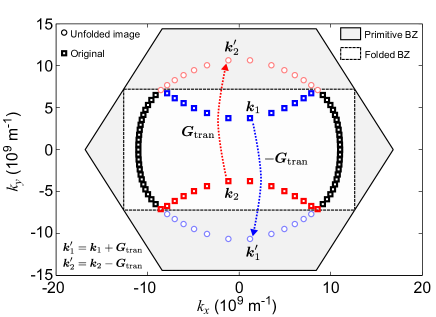
Figure 6: Plot of computed ZA phonon modes at $\omega=33$ meV in the folded Brillouin zone (BZ) and their image points in the unfolded primitive BZ. The locus of the phonon channels (square symbols) within the folded BZ forms the shape of a dual-blade ax head while the shape of the locus of the phonon channels within the primitive BZ is approximately circular.

IV.2 Chirality dependence of phonon boundary scattering in graphene

We study the effects of the edge chirality or orientation on the boundary scattering of low-energy flexural acoustic (ZA) phonons in graphene. It is shown by Wei, Chen and Dames in Ref. (Wei et al., 2012) using wave packet dynamics simulations that the scattering of ZA phonons by the armchair edge can lead to what they call “wave packet splitting”, a phenomenon in which the incoming wave packet is split into two or more outgoing components with dissimilar wave vectors and back-scattered wave packets are generated after scattering. In the scattering framework, the two outgoing wave packet components correspond to having two outgoing phonon channels in which the transition probability is not zero. Wave packet splitting is however not observed in their simulations of scattering with the zigzag edge, (Wei et al., 2012) suggesting that the edge chirality exerts a profound effect on the phonon scattering specularity. Additional evidence of this edge chirality dependence is provided by molecular dynamics simulations showing that the thermal conductivity is lower for armchair-edge graphene nanoribbons than for zigzag-edge graphene nanoribbons. (Hu et al., 2009) To explain their findings, (Wei et al., 2012) Wei, Chen and Dames attribute the wave packet splitting to “the deeper symmetry properties of armchair and zigzag edges of the hexagonal graphene lattice”.

To understand the physics underlying this phenomenon more precisely, we investigate the edge scattering of ZA phonons by using our $S$-matrix approach to compute the transition probabilities between an incoming ZA phonon channel incident on the edge and the outgoing (reflected) ZA phonon channels for different edge chirality types. The scope of our investigation is limited to ZA phonons because the wave packet splitting of the longitudinal (LA) and transverse acoustic (TA) phonons can also arise from polarization conversion which does not affect ZA phonons but can obscure the specularity dependence on edge chirality. Our simulated system comprises a semi-infinite graphene sheet that is terminated on the right like in Figs. 7(a) and 7(d). In our scattering calculations, we set $\omega=33$ meV or $5\times 10^{13}$ rad/s and set the incident phonon to be at either normal ($k_{y}=0$) or oblique ($k_{y}\neq 0$) incidence.

IV.2.1 Zigzag edge

Figure 7(b) shows the transition probability distribution along the reciprocal-space locus of the outgoing ZA phonon channels (solid square symbols) as well as the position of the incoming phonon channel at $\boldsymbol{k_{1}}$ (solid circle), which is at normal incidence ($k_{y}=0$) to the zigzag-edge boundary as shown in Fig. 7(a). We find that incident phonon is specularly scattered, i.e. $\mathcal{P}(\boldsymbol{k_{1}})=1$, to the outgoing phonon channel at $\boldsymbol{\bar{k}_{1}}=\sigma\boldsymbol{k_{1}}$, where $\sigma$ is the operator corresponding to the reflection $(k_{x},k_{y})\rightarrow(-k_{x},k_{y})$ in reciprocal space, given the computed transition probability of $P(\boldsymbol{k_{1}}\rightarrow\boldsymbol{\bar{k}_{1}})=1.000$. Figure 7(c) shows the transition probability distribution for the incoming phonon channel at $\boldsymbol{k_{2}}$ which is at an oblique incidence ($k_{y}\neq 0$) to the boundary. The calculation also yields $P(\boldsymbol{k_{2}}\rightarrow\boldsymbol{\bar{k}_{2}})=1.000$ for $\boldsymbol{\bar{k}_{2}}=\sigma\boldsymbol{k_{2}}$, indicating that the phonon is also specularly scattered. These results are consistent with the findings in Ref. (Wei et al., 2012) where it is shown that ZA phonon scattering with the zigzag edge is always specular regardless of the angle of incidence.

IV.2.2 Armchair edge

We repeat our calculations for ZA phonon scattering with the armchair edge as shown in Fig. 7(d). At normal incidence to the armchair edge, the incident phonon at $\boldsymbol{k_{3}}$ is specularly scattered to the outgoing phonon channel $\boldsymbol{\bar{k}_{3}}=\sigma\boldsymbol{k_{3}}$ since $P(\boldsymbol{k_{3}}\rightarrow\boldsymbol{\bar{k}_{3}})=1.000$ as shown in Fig. 7(e). However, at oblique incidence, the scattering of the incoming phonon channel at $\boldsymbol{k_{4}}$ is only partially specular as $P(\boldsymbol{k_{4}}\rightarrow\boldsymbol{\bar{k}_{4}})=0.264$ for $\boldsymbol{\bar{k}_{4}}=\sigma\boldsymbol{k_{4}}$ and the incident phonon is also backscattered to a second outgoing phonon channel at $\boldsymbol{\bar{k}_{5}}$ with $P(\boldsymbol{k_{4}}\rightarrow\boldsymbol{\bar{k}_{5}})=0.736$. There are no other outgoing channels to which the incident phonon is scattered because the total transition probability of these two outgoing channels is $P(\boldsymbol{k_{4}}\rightarrow\boldsymbol{\bar{k}_{4}})+P(\boldsymbol{k_{4}}\rightarrow\boldsymbol{\bar{k}_{5}})=1.000$. This splitting of the incident ZA phonon to two outgoing ZA phonon channels after scattering with the armchair edge is qualitatively consistent with the wave packet splitting observed in Ref. (Wei et al., 2012).

To explain the partial scattering specularity of the incident phonon at $\boldsymbol{k_{4}}$, we note that the $y$ component of $\boldsymbol{\bar{k}_{5}}-\boldsymbol{\bar{k}_{4}}$, which is the difference in the reciprocal-space position of the outgoing phonon channels at $\boldsymbol{\bar{k}_{4}}$ and $\boldsymbol{\bar{k}_{5}}$, is equal to $\boldsymbol{G}_{\text{tran}}$ which characterizes the periodicity of the armchair edge as well as that of the supercell [Fig. 7(d)] in the transverse ($y$) direction. To make this clearer, we plot in Fig. 7(f) the point $\boldsymbol{\bar{k}_{5}^{\prime}}=\boldsymbol{\bar{k}_{5}}+\boldsymbol{G}_{\text{tran}}$ which is collinear with $\boldsymbol{k_{4}}$ and $\boldsymbol{\bar{k}_{4}}$. More generally, this implies that any elastic phonon scattering by the edge must satisfy the conservation condition

$$\hat{\boldsymbol{y}}\cdot(\boldsymbol{k}_{\text{in}}-\boldsymbol{k}_{\text{out}})=m|\boldsymbol{G}_{\text{tran}}|$$ (61)

where $m\in\mathbb{Z}$ and $\boldsymbol{k}_{\text{in}}$ ($\boldsymbol{k}_{\text{out}}$) is the wave vector of the incoming (outgoing) phonon channel.

Therefore, given Eq. (61), we can explain why phonon scattering by the armchair edge is fully specular in Fig. 7(e) and only partially specular in Fig. 7(f). In Fig. 7(e) where the incoming phonon at $\boldsymbol{k_{3}}$ is at normal incidence to the boundary, the only outgoing phonon channel that satisfies Eq. (61) is at $\boldsymbol{\bar{k}_{3}}$ and hence, the incident phonon undergoes fully specular scattering. On the other hand, when the incoming phonon is at $\boldsymbol{k_{4}}$, there are two outgoing phonon channels ($\boldsymbol{\bar{k}_{4}}$ and $\boldsymbol{\bar{k}_{5}}$) that satisfy Eq. (61), such that $\hat{\boldsymbol{y}}\cdot(\boldsymbol{k_{4}}-\boldsymbol{\bar{k}_{4}})=0$ and $\hat{\boldsymbol{y}}\cdot(\boldsymbol{k_{4}}-\boldsymbol{\bar{k}_{5}})=|\boldsymbol{G}_{\text{tran}}|$, resulting in a “splitting” of the incoming phonon.

Along the same lines, we can also explain the full specularity of ZA phonon scattering and the absence of wave packet splitting for the zigzag edge. The greater symmetry of the zigzag edge means that its $|\boldsymbol{G}_{\text{tran}}|$ is larger than the $|\boldsymbol{G}_{\text{tran}}|$ of the armchair edge since $|\boldsymbol{G}_{\text{tran}}|=\frac{2\pi}{\sqrt{3}a}$ and $\frac{2\pi}{3a}$ for the zigzag and armchair edge, respectively, where $a$ is the carbon-carbon bond length. This can also be seen when we compare the width of the folded BZ along the $k_{y}$-axis in Figs. 7(b) and 7(e). Hence, the conservation condition in Eq. (61) is more restrictive for the zigzag edge because its larger $|\boldsymbol{G}_{\text{tran}}|$ allows for only one outgoing phonon channel when $\omega=33$ meV.

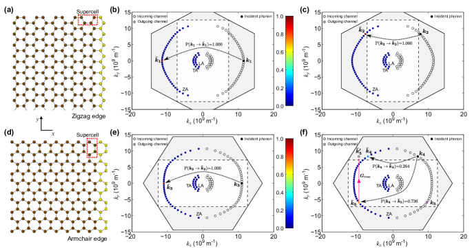
Figure 7: Diagram of the smooth graphene (a) zigzag and (d) armchair edge structure along the $y$ direction. The bulk and edge C atoms are colored brown and yellow, respectively. For the zigzag edge, the two-dimensional distribution of the incoming and outgoing (reflected) phonon channels at $\omega=33$ meV in the first Brillouin zone (BZ) are shown for an incident flexural phonon at (b) $\boldsymbol{k_{1}}$ and (c) $\boldsymbol{k_{2}}$. The locus of channels can be placed in three ‘rings’ corresponding to the longitudinal acoustic (LA), transverse acoustic (TA) and flexural acoustic (ZA) phonons. In addition to the first BZ, we also draw the outline of the folded BZ (dashed lines) corresponding to the supercell shown in (a). The associated transition probabilities for the outgoing reflected channels are indicated in color. The incident phonons are specularly scattered to the channels at $\boldsymbol{\bar{k}_{1}}$ and $\boldsymbol{\bar{k}_{2}}$. For the armchair edge, the distributions of the incoming and outgoing phonon channels are similarly shown for the incident phonon at (e) $\boldsymbol{k_{3}}$ and (f) $\boldsymbol{k_{4}}$. The phonon at $\boldsymbol{k_{3}}$ is specularly scattered to $\boldsymbol{\bar{k}_{3}}$ but the phonon at $\boldsymbol{k_{4}}$ is scattered into two channels at $\boldsymbol{\bar{k}_{4}}$ and $\boldsymbol{\bar{k}_{5}}$, with the $\boldsymbol{k_{4}}\rightarrow\boldsymbol{\bar{k}_{5}}$ transition probability greater than the $\boldsymbol{k_{4}}\rightarrow\boldsymbol{\bar{k}_{4}}$ transition probability. The point at $\boldsymbol{\bar{k}_{5}^{\prime}}=\boldsymbol{\bar{k}_{5}}+\boldsymbol{G}_{\text{tran}}$ is collinear with $\boldsymbol{k_{4}}$ and $\boldsymbol{\bar{k}_{4}}$ as a consequence of Eq. (61).

IV.3 Effect of graphene edge chirality and isotopic disorder on ZA phonon specularity

IV.3.1 Ordered edges

We use our $S$-matrix method to study how the ZA phonon boundary scattering specularity ($\mathcal{P}$) varies systematically with frequency ($\omega$) and wave vector ($\boldsymbol{k}$) for different edge chirality configurations. The specularity parameter distribution of the incoming flexural acoustic (ZA) phonons is computed at $\omega=l\omega_{0}$, where $\omega_{0}=6.6$ meV or $10^{13}$ rad/s and $l=1,\ldots,6$, in Fig. 8 for: (a) the ideal zigzag edge with $N=42$ unit cells or 84 atoms and (b) the ideal armchair edge with $N=24$ unit cells or 96 atoms in the transverse direction. At each frequency point, the locus of all the incoming ZA phonons is represented by a constant-frequency arc, as shown in Fig. 8, and the loci form a concentric arrangement of arcs with the innermost and outermost arc corresponding to $\omega=\omega_{0}$ and $\omega=6\omega_{0}$, respectively.

Figure 8(a), which corresponds to the ideal zigzag edge, shows that the specularity is perfect ($\mathcal{P}=1$) as expected for all incoming ZA phonons in the frequency range studied, confirming the conservation condition in Eq. (61). However, in Fig. 8(b) which corresponds to the ideal armchair edge, the the ZA phonon specularity varies with the frequency $\omega$ and wave vector $\boldsymbol{k}=(k_{x},k_{y})$, in agreement with the findings of Ref. (Wei et al., 2012). Figure 8(b) shows that the variation in specularity with $\boldsymbol{k}$ becomes more pronounced at larger $\omega$. In each constant-frequency arc in Fig. 8(b) for $\omega=4\omega_{0}$ to $6\omega_{0}$, $\mathcal{P}(\boldsymbol{k})$ approaches its minimum as $k_{y}$ approaches $\pm\frac{1}{2}|\boldsymbol{G}_{\text{tran}}|$ as indicated in Fig. 8(b). The existence of this minimum at a particular incident angle is reported but not explained in Ref. (Wei et al., 2012).

For the specularity minimum at $k_{y}=\pm\frac{1}{2}|\boldsymbol{G}_{\text{tran}}|$, there are two outgoing channels at $\boldsymbol{\bar{k}}$ and $-\boldsymbol{k}$. Figure 8(b) shows that as we increase the frequency, the $\boldsymbol{k}\rightarrow-\boldsymbol{k}$ transition, which corresponds to the reversal of the phonon trajectory such that the angle of incidence is equal to the negative of the angle of reflection, becomes increasingly more probable. This implies that at high phonon frequencies, the a greater proportion of the phonon momentum in the $y$-direction is lost due to scattering with the ideal armchair edge.

IV.3.2 Disordered edges

Given the role of the edge translational symmetry in the ZA phonon scattering specularity, it would be interesting to see the effect of the loss of that symmetry on phonon specularity. To break the translational symmetry of the graphene edge, we randomly replace 25 percent of the edge¹²C atoms with ²⁴C atoms [Figs. 8(a) and 8(d)] to create isotopic disorder along the edges.

Figure 8 shows the specularity parameter distribution at $\omega=l\omega_{0}$, where $l=1,\ldots,6$, for incoming ZA phonon channels at: (a,b) the zigzag edge with $N=42$ unit cells or 84 atoms and (c,d) the armchair edge with $N=24$ unit cells or 96 atoms in the transverse direction. The specularity distributions for the mass-disordered edges in Fig. 8(b) and (d) are obtained after averaging over 20 realizations of disorder while the distributions in Figs. 8(a) and 8(c) have no disorder and represent the baseline specularity values.

A comparison of Figs. 8(a) and 8(c) shows that the $\mathcal{P}(\boldsymbol{k})=1$ result no longer holds in the disordered zigzag edge. We observe that the specularity decreases as the frequency and the angle of incidence decrease. This dependence on the angle of incidence is unexpected as models of surface roughness scattering (Ziman, 1960; Maznev, 2015) suggest that the specularity should decrease monotonically with the angle of incidence. This suggests that the effect of edge disorder is different from that of edge roughness and that caution should be exercised when using specularity approximations based on surface roughness scattering.

In Fig. 8(d) at large $\omega$ ($\omega=l\omega_{0}$ for $l=4$ to $6$), we observe that the specularity parameter $\mathcal{P}(\boldsymbol{k})$ is maximum at normal incidence to the edge but decreases as the angle of incidence increases before reaching its minimum when $k_{y}=\pm\frac{1}{2}|\boldsymbol{G}_{\text{tran}}|$ like in Fig. 8(c). Comparing Figs. 8(c) and (d), we find that the isotopic disorder at the armchair edge reduces $\mathcal{P}(\boldsymbol{k})$, with the decrease in $\mathcal{P}(\boldsymbol{k})$ becoming larger at higher frequency and angle of incidence, similar to the trend observed for the zigzag edge.

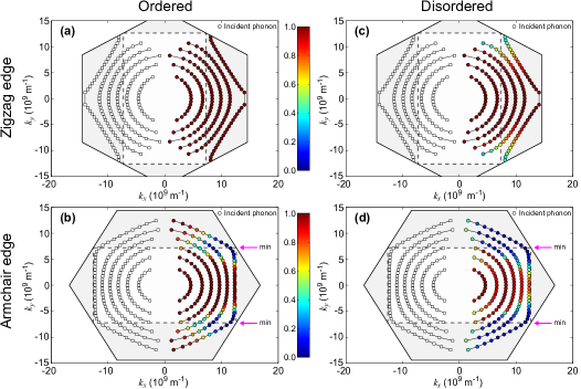
Figure 8: Plot of the specularity parameter value $\mathcal{P}$ distribution within the Brillouin zone for incoming (incident) flexural acoustic (ZA) phonon channels (filled circles) at $\omega=l\omega_{0}$, where $\omega_{0}=6.6$ meV or $10^{13}\ \text{rad s}^{-1}$ and $l=1,\ldots,6$, for the (a) ordered zigzag, (b) ordered armchair, (c) disordered zigzag and (d) disordered armchair edge, computed using Eq. (27). The outgoing ZA phonon channels are represented by hollow square symbols. The ZA phonon channels are arranged in concentric constant-$\omega$ arcs. The $\mathcal{P}(\boldsymbol{k})$ minima at each $\omega$ lie along the $k_{y}=\pm\frac{1}{2}|\boldsymbol{G}_{\text{tran}}|$ line (labeled ‘min’) for both the isotopically ordered and disordered armchair edge.

V Summary and conclusion

We have described the improvement of the atomistic Green’s function (AGF) method for treating individual phonon transmission and reflection, and shown explicitly how the phonon transmission and reflection matrices can be determined numerically and used to construct the unitary $S$ matrix that characterizes scattering by the interface and treats bulk phonon modes as scattering channels. In our AGF-based $S$-matrix approach, the scattering amplitude between the phonon channels is determined from the corresponding $S$-matrix element and yields the transition probability for the forward (transmission) or backward (reflection) scattering process. We illustrate the advantages of our new approach by first applying it to the example of phonon scattering at the junction of two isotopically different (8,8) carbon nanotubes. The $S$-matrix approach allows us to determine the dependence of the phonon transmission and reflection on frequency, polarization and phonon velocity. We also analyze the transition probability for individual scattering processes as well as describe the role of intra and inter-subband processes in phonon reflection.

We also illustrate the utility of the method by applying it to the study of phonon reflection from a graphene edge. We take advantage of the transverse periodic boundary condition to partition the system into its Fourier components for more efficient computation of matrix variables such as the surface Green’s function. For clarity, the scattering channels are mapped to the bulk phonon modes of graphene using the Boykin-Klimeck zone-unfolding technique. Our numerical calculations reveal that unlike the zigzag edge, phonon scattering with the armchair edge is only partially specular because of the symmetry difference between the armchair edge and the bulk lattice. We also find that the specularity varies with wave vector and frequency and decreases as expected when isotopic disorder is introduced to the edge.

Potentially, the application of our AGF-based $S$-matrix method in the atomistic simulations of other interfaces can provide a similarly detailed picture of phonon transmission and reflection, and shed light on the relationship between phonon scattering and the atomistic structure of the interface or surface. The method may also be incorporated into multiscale models of phonon and thermal conduction in heterogeneous solids with interfaces (Singh et al., 2011) by combining it with the transport models based on the Boltzmann transport equation. The method can also be used to estimate phonon specularity in transport models of low-dimensional systems (e.g. silicon nanowires or graphene nanoribbons) in which edge scattering is important for momentum relaxation. In addition, the formalism presented in this paper may be applicable on its own to the numerical simulation of scattering in linear systems (e.g. photonic crystals (Joannopoulos et al., 2008)) that have a lattice structure and are second order in time.