Two-dimensional composite solitons in a spin-orbit-coupled Fermi gas in free space

Abstract

We address a possibility of creating soliton states in oblate binary-fermionic clouds in the framework of the density-functional theory, which includes the spin-orbit coupling (SOC) and nonlinear attraction between spin-up and down-polarized components of the spinor wave function. In the limit when the inter-component attraction is much stronger than the effective intra-component Pauli repulsion, the resulting model also represents a system of Gross-Pitaevskii equations for a binary Bose-Einstein condensate including the SOC effect. We show that the model gives rise to two-dimensional quiescent composite solitons in free space. A stability region is identified for solitons of the mixed-mode type (which feature mixtures of zero-vorticity and vortical terms in both components), while solitons of the other type, semi-vortices (with the vorticity carried by one component) are unstable. Due to breaking of the Galilean invariance by SOC, the system supports moving solitons with velocities up to a specific critical value. Collisions between moving solitons are briefly considered too. The collisions lead, in particular, to a quasi-elastic rebound, or an inelastic outcome, which features partial merger of the solitons.

1 Introduction

Experimental and theoretical research of degenerate fermionic gases has drawn much interest, as their confining geometry, size, and interaction strength can be varied in broad ranges [1, 2, 3, 4, 5].With the help of many-body Hamiltonian models, phase diagrams of quasi-one-dimensional (1D) Fermi systems were produced in several settings [6, 7, 8, 9, 10, 11, 12, 13]. The mean-field theory, which essentially amounts to the establishment of the Gross Pitaevskii equations (GPEs), provides a very accurate dynamical model for bosonic gases [14]. Models for Fermi superfluids and Fermi-Bose mixtures were elaborated, under specific conditions, in the form of the density-functional theory [15]-[27]. Using these theoretical models, various nonlinear effects in degenerate quantum gases were studied, such as generation of different types of vortex rings [28, 29, 30], shock waves [31, 32], and chaotic dynamics [33]. Other nonlinear effects in degenerate Fermi systems, as well as in Bose-Fermi mixtures, were elaborated in Refs. [34, 35, 36, 37, 38, 39, 40, 41, 42].

Creation of stable 2D and 3D solitons, both fundamental and vortical ones, is a well-known fundamental problem in nonlinear optics and Bose-Einstein condensates (BECs). Induced by the Kerr effect in optics and attractive inter-atomic interactions in BEC, the basic cubic self-focusing nonlinearity builds solitons which are completely unstable because of the critical and supercritical collapse in 2D and 3D settings, respectively [43, 44, 45]. Several possibilities for the stabilization of the multidimensional solitons were theoretically developed, the most ubiquitous one being the use of lattice potentials [46, 47, 48]. Recently, it was demonstrated that both 2D [49, 50, 51, 52, 53, 54, 55, 56, 57, 58] and 3D [59] two-component solitons in the free space with the cubic self-focusing can be stabilized with the help of spin-orbit coupling (SOC) in BEC (see a summary in a recent brief review [60]). The SOC effect is represented, in experimentally implemented models of bosonic [61, 62, 63, 64, 65, 66] and fermionic [67, 68] gases, by linear terms coupling the two components through first spatial derivatives, see also reviews [69, 70, 71, 72]. It is essential to stress that, while most experimental works for SOC were carried out in effectively 1D settings, the realization of the SOC in 2D geometry was demonstrated too, for bosons [73] and fermions [74] alike. In 2D models, the SOC terms lift the specific conformal invariance of the GPEs with cubic self-attraction, which is responsible for the onset of the critical collapse. As a result, in this case the addition of the SOC to the GPE system creates the otherwise missing ground state in the form of semi-vortex (SV) solitons with one zero-vorticity (fundamental) and one vortical components, provided that the self-attraction is stronger than the cross-attraction. In the opposite case, SVs are unstable, while the ground state is represented by the mixed-mode (MM) state, which combines fundamental and vortical terms in both components. Furthermore, the SVs and MMs remain stable when, respectively, the cross- or self-interaction is repulsive, the self-trapping being provided by the stronger self- (cross-) attraction for SVs (MMs) [55].

The aim of the present work is to obtain soliton solutions in the model of an oblate (quasi-2D) Fermi superfluid, based on the known 2D density-functional equations [34, 35, 36, 37, 38, 39, 40, 41, 42], to which SOC terms are added. We demonstrate that the system produces quiescent composite solitons in the free 2D space. Further, because the Galilean invariance of the system is broken by the SOC terms, generating moving solitons from the quiescent ones is a nontrivial issue too. We find that moving solitons can be created, with velocities limited by a critical value, which depends on the strength of the spin-orbit coupling as well as on soliton’s norm. Collisions between moving solitons are also addressed, by means of direct simulations.

The rest of the paper is organized as follows. The model is introduced in Section 2. Numerical results for quiescent and moving solitons are presented in Sections 3 and 4, respectively, the latter one also including the consideration of collisions between moving solitons. The paper is concluded by Section 5.

(a)	(b)
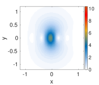
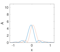
(c)	(d)
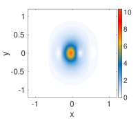
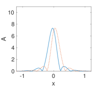
(e)	(f)

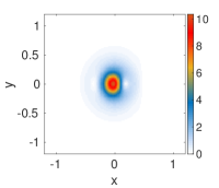
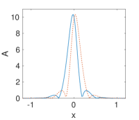
Figure 1: Left: contour plots of $|\Psi_{1}(\mathbf{r},t)|$ for stable stationary MM solutions in the $\left(x,y\right)$ plane, as produced by the full system based on Eqs. (1). Right: profiles of both field components in the stationary solutions, $|\Psi_{1}(\mathbf{r},t)|$ and $|\Psi_{2}(\mathbf{r},t)|$ (blue solid and red dotted lines, respectively) in the cross-section $y=0$. Panels (a,b), (c,d) and (e,f) correspond to total norms $N=8.0$, $9.5$, and $11.0$, respectively. Fixed parameters are $\gamma=1$, $\varepsilon=0$ and $\lambda=9$.

2 The model

The system of 2D density-functional equations for the spinor wave function, $\Psi(\mathbf{r},t)=\left(\Psi_{1}(\mathbf{r},t),\Psi_{2}(\mathbf{r},t)\right)$, of the binary Fermi gas, which include contact attraction between the two components (spin-up and down atomic states) with strength $\gamma>0$, the effective self-repulsive Pauli nonlinearity, SOC terms of the Rashba type [75, 76] with strength $\lambda$, and Zeeman splitting with strength $\varepsilon$ are written in the scaled form as

$$i\frac{{\partial{\Psi_{1}}}}{{\partial t}}=-\frac{1}{2}{\nabla^{2}}{\Psi_{1}}+{\left|{{\Psi_{1}}}\right|^{4/3}}{\Psi_{1}}-\gamma{\left|{{\Psi_{2}}}\right|^{2}}{\Psi_{1}}+\lambda\left({\frac{{\partial{\Psi_{2}}}}{{\partial x}}-i\frac{{\partial{\Psi_{2}}}}{{\partial y}}}\right)+\varepsilon{\Psi_{1}\,,}$$

$$i\frac{{\partial{\Psi_{2}}}}{{\partial t}}=-\frac{1}{2}{\nabla^{2}}{\Psi_{2}}+{\left|{{\Psi_{2}}}\right|^{4/3}}{\Psi_{2}}-\gamma{\left|{{\Psi_{1}}}\right|^{2}}{\Psi_{2}}-\lambda\left({\frac{{\partial{\Psi_{1}}}}{{\partial x}}+i\frac{{\partial{\Psi_{1}}}}{{\partial y}}}\right)-\varepsilon{\Psi_{2}.}$$ (1)

Starting from the full 3D system, one can derive the effectively 2D system by eliminating the third direction, in which the gas is assumed to be strongly confined by an external potential (see, e.g., work [21]). Along with the Hamiltonian and 2D momentum, the system conserves the total norm, which is proportional to the number of atoms in the degenerate gas,

$$N=\int{\int{\left({{{\left|{{\Psi_{1}}\left({\mathbf{r},t}\right)}\right|}^{2}}+{{\left|{{\Psi_{2}}\left({\mathbf{r},t}\right)}\right|}^{2}}}\right)}}{d^{2}}r.$$ (2)

It is relevant to stress that the local interaction between the polarized spin-up and down fermions may be controlled, as concerns its sign and strength, by means of the Feshbach resonance [77, 78].

In the limit case or of large atomic density, $\gamma\left|\Psi_{1,2}\right|^{2/3}\gg 1$, the Pauli self-repulsion may be neglected, reducing Eq. (1) to

$$i\frac{{\partial{\Psi_{1}}}}{{\partial t}}=-\frac{1}{2}{\nabla^{2}}{\Psi_{1}}-\gamma{\left|{{\Psi_{2}}}\right|^{2}}{\Psi_{1}}+\lambda\left({\frac{{\partial{\Psi_{2}}}}{{\partial x}}-i\frac{{\partial{\Psi_{2}}}}{{\partial y}}}\right)+\varepsilon{\Psi_{1},}$$

$$i\frac{{\partial{\Psi_{2}}}}{{\partial t}}=-\frac{1}{2}{\nabla^{2}}{\Psi_{2}}-\gamma{\left|{{\Psi_{1}}}\right|^{2}}{\Psi_{2}}-\lambda\left({\frac{{\partial{\Psi_{1}}}}{{\partial x}}+i\frac{{\partial{\Psi_{1}}}}{{\partial y}}}\right)-\varepsilon{\Psi_{2}.}$$ (3)

The same system (3) applies to a binary bosonic condensate dominated by the inter-species attraction, which may also be enhanced by means of the Feshbach resonance [55].

Using the remaining scaling invariance of Eqs. (1) and (3), we fix $\gamma=1$ (the case of $\gamma=0$ is irrelevant here, as in that case the system cannot produce bright solitons), while the SOC and Zeeman strengths $\lambda$ and $\varepsilon$ remain irreducible parameters in the full system (1). In the reduced system (3), $\lambda$ it may be scaled to any fixed value, the only remaining free parameter being $\varepsilon$.

The spectrum of small-amplitude plane waves, generated by the linearization of Eqs. (1) or (3) for $\Psi_{1,2}\sim\exp\left(i\mathbf{k}\cdot\mathbf{r}-i\mu t\right)$, where $\mathbf{k}$ is the wave vector and $\mu$ a real chemical potential, gives rise to two branches [79]:

$$\mu=\frac{k^{2}}{2}\pm\sqrt{\lambda^{2}k^{2}+\varepsilon^{2}}.$$ (4)

Solitons may exist at values of $\mu$ which are not covered by Eq. (4) with real $k^{2}\geq 0$, i.e., at

$$\mu<-\frac{1}{2}\left(\lambda^{2}+\frac{\varepsilon^{2}}{\lambda^{2}}\right),\leavevmode\nobreak\ \mathrm{if}\leavevmode\nobreak\ \leavevmode\nobreak\ \lambda^{2}>|\varepsilon|,$$

$$\mu<-|\varepsilon|,\leavevmode\nobreak\ \mathrm{if}\leavevmode\nobreak\ \leavevmode\nobreak\ \lambda^{2}<|\varepsilon|.$$ (5)

Stationary states with chemical potential $\mu$ are sought for as

$$\Psi_{1,2}=e^{-i\mu t}U_{1,2}\left(x,y\right),$$ (6)

where complex amplitude functions $U_{1,2}$ satisfy equations

$$\mu U_{1}=-\frac{1}{2}{\nabla^{2}U_{1}}+{\left|{{U_{1}}}\right|^{4/3}U_{1}}-\gamma{\left|{{U_{2}}}\right|^{2}U_{1}}+\lambda\left({\frac{{\partial U{{}_{2}}}}{{\partial x}}-i\frac{{\partial U{{}_{2}}}}{{\partial y}}}\right)+\varepsilon{U_{1},}$$

$$\mu U_{2}=-\frac{1}{2}{\nabla^{2}U_{2}}+{\left|{{U_{2}}}\right|^{4/3}U_{2}}-\gamma{\left|{{U_{1}}}\right|^{2}U_{2}}-\lambda\left({\frac{{\partial U{{}_{1}}}}{{\partial x}}+i\frac{{\partial U{{}_{1}}}}{{\partial y}}}\right)-\varepsilon{U_{2}.}$$ (7)

We have produced stationary states, solving Eqs. (1) and (3) by means of the well-known imaginary-time method [80, 81], and stability of the stationary states was then tested by means of real-time simulations of their perturbed evolution. This was done by means of the fourth-order Runge-Kutta method for marching in time with step $\Delta t=10^{-4}$, handling the spatial derivatives by means of the centered second-order finite-difference method with $\Delta x=\Delta y=0.025$, in terms of the scaled variables. The numerical solutions were obtained in a 2D domain, defined as $|x|,|y|<4$, with zero boundary conditions, the size of the solitons always being much smaller than the domain width. Reliability of the numerical results was checked by reproducing them with smaller values of $\Delta t$ and $\Delta x$, $\Delta y$, as well as with different sizes of the integration domain.

3 Stationary mixed-mode solitons

3.1 The full model

(a)	(b)
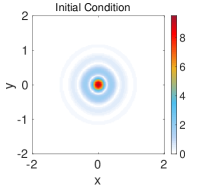
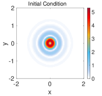
(c)	(d)
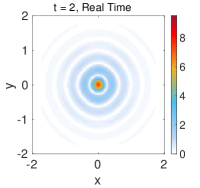
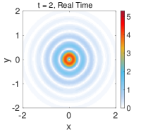
(e)	(f)

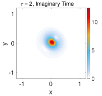
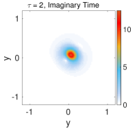
Figure 2: Contour plots of $|\Psi_{1}(\mathbf{r},t)|$ and $|\Psi_{2}(\mathbf{r},t)|$ (left and right panels, respectively) of an unstable SV. $(\mathrm{a,b})$ The SV state produced by the evolution in imaginary time, $t=i\tau$, from input (9), at $\tau=27.5$. $(\mathrm{c,d})$ The result of the unstable evolution in real time from $t=0$ to $t=2$. $(\mathrm{e,f})$ The result of the additional evolution of the SV from panels $\left(\mathrm{a,b}\right)$ in the imaginary time, $\Delta t=i\Delta\tau$, at $\Delta\tau=2$, which demonstrates spontaneous rearrangement of the SV into a stable MM. Fixed parameters are $N=11.5$, $\gamma=1$, $\varepsilon=0$ and $\lambda=9$.

The analysis is initiated by dropping the Zeeman splitting, i.e., setting $\varepsilon=0$, but keeping the Pauli-repulsion terms in Eqs. (1). In this system, self-trapped states of the MM type were generated by imaginary-time simulations, initiated with the input combining vorticities $(0,-1)$ and $(0,+1)$ in the two components, cf. Ref. [49]:

$$\Psi_{1}^{(0)}(\mathbf{r})=A_{1}\exp(-\alpha_{1}r^{2})-A_{2}r\exp(-i\theta-\alpha_{2}r^{2}),$$

$$\Psi_{2}^{(0)}(\mathbf{r})=A_{1}\exp(-\alpha_{1}r^{2})+A_{2}r\exp(i\theta-\alpha_{2}r^{2}).$$ (8)

Subsequently, real-time simulations reveal the stability of the stationary MMs in their full existence domain, in both the full and reduced models, based on Eqs. (1) and (3), respectively. Figure 1 shows typical contour plots and cross-section profiles of stationary solitons of the MM type, obtained for three different values of norm (2). Naturally, as $N$ increases, making the cross-attraction stronger, the solitons’ amplitude increases too.

In addition, 2D solitons of the SV type were produced too, with an input carrying vorticity $0$ in one component and $1$ in the other, as suggested by work [49]. In this case, Eqs. (3.1) and (8) are reduced to

$$\Psi_{1}^{(0)}(\mathbf{r})=A_{1}\exp(-\alpha_{1}r^{2}),$$

$$\Psi_{2}^{(0)}(\mathbf{r})=A_{2}r\exp(i\theta-\alpha_{2}r^{2}).$$ (9)

However in contrast to the MMs, the so built SVs are completely unstable, which resembles the result for the bosonic binary condensate, obtained in work [55], in the case of the repulsive self-interaction and attractive cross-interaction, combined with SOC.

The instability of the SV is illustrated in Fig. 2, which displays the evolution of its two components. In particular, panels (a,b) show the result of the evolution in the imaginary time, $t=i\tau$, of input (9), at $\tau=27.5$. The SV shape is maintained by the evolution up to this value of $\tau$. However, if this SV is used as the initial state for the real-time simulations, panels (c,d) show that the result is instability, which causes decay of the SV. Further, if the imaginary-time simulation is continued from $\tau=27.5$, which corresponds to panels (a,b), by adding $\Delta\tau=2$, the ostensibly stable SV spontaneously rearranges into a truly stable MM, see panels (e,f) (the value of the Hamiltonian corresponding to the emerging MM is $H_{\mathrm{MM}}=-750.1$, which is smaller than the SV’s original value, $H_{\mathrm{SV}}=-475.3$, which confirms that the MM is stable, while the SV is not). The stability of this MM is confirmed by real-time simulations (not shown here in detail).

Figure 3 displays the dependence of the MM’s chemical potential, $\mu$, and amplitude, $A_{\max}$ [the largest value of $\left|U_{1,2}(x,y)\right|$, in Eq. (6)], on norm $N$ and SOC strength $\lambda$. The stability of the MMs complies with the fact that all the $\mu(N)$ curves satisfy the Vakhitov-Kolokolov criterion, which is a well-known necessary condition for the existence of all self-trapped states created by attractive interactions [82, 43, 44]. Further, Fig. 3(b) clearly shows that, for given SOC strength $\lambda$, the MM exists at $N>N_{\min}$ (where $N_{\min}$ is the value of $N$ at which the amplitude drops to very small values in Fig. Fig. 3(b)), and vice versa: for given $N$, it exists at $\lambda$ exceeding a certain finite minimum value, $\lambda_{\min}$. At $N<N_{\min}$, solitons cannot self-trap in the full system (1), as in that case the Pauli self-repulsion in each component dominates over the inter-component attraction.

To summarize these findings, Fig. 4 shows the MM stability region in the $\left({\lambda,N}\right)$ plane. In particular, the nonexistence of MMs at too small and too large values of $N$, observed in the latter figure, is consistent with the same features demonstrated by Fig. 3(b).

Similar to the situation analyzed in the binary BEC [49], the MM structure is characterized by spatial separation, $D$, in the $x$ direction, between density peaks of the two components. $D$ is plotted, as a function of $N$, for different fixed values of $\lambda$ in Fig. 5. Naturally, the increase of $N$ strengthens the attraction between the components, thus leading to decrease of $D$.

(a)	(b)

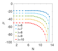
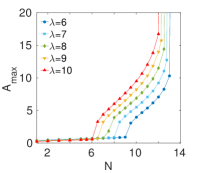
Figure 3: Chemical potential, $\mu$, and the amplitude, $A_{\max}$ of stable mixed modes in the full system (1) versus the norm, $N$, for different fixed values of the SOC strength, $\lambda$. The drop of $A_{\max}$ to very small values at $N=N_{\min}$ in (b) (e.g., $N_{\min}\approx 6$ at $\lambda=10$) implies that the MM soliton suffers delocalization into a state which tends to occupy the entire integration domain). Other fixed parameters are the same as in Fig. 1: $\gamma=1$, $\varepsilon=0$.

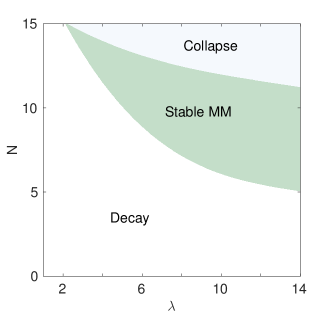
Figure 4: The stability area for MMs in the plane of the SOC strength, $\lambda$, and total norm, $N$. In the “collapse” area, the cubic cross-attraction is strong enough to drive the system towards the collapse. MM-shaped inputs decay below the stability area, where the attractive interaction is insufficient to secure the self-trapping.

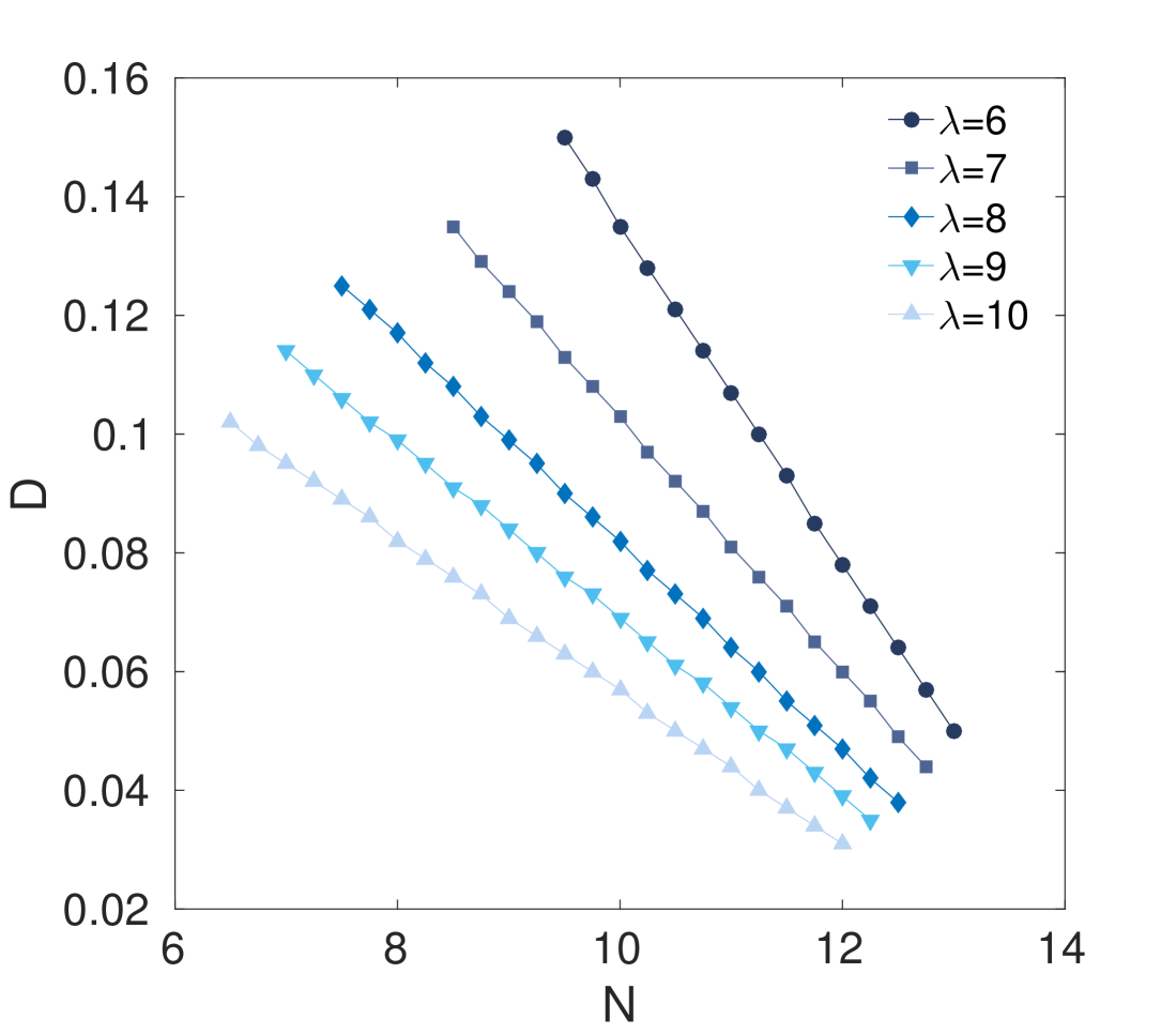
Figure 5: Separation $D$ (in the $x$ direction) between positions of density maxima in the two components of the mixed modes, as a function $N$ for different fixed values of $\lambda$. Other parameters are the same as in Fig. 1.

(a)	(b)

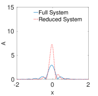
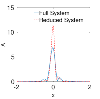
Figure 6: Comparison of cross-section profiles of $|\Psi_{1}(x)|$ at $y=0$ between the MM solitons produced by the the full and reduced systems (solid and dashed lines, respectively). The profiles are produced for $N=7.0$ (a) and $N=9.25$ (b). The other parameters are the same as in Fig. 1.

3.2 The reduced system and one with the Zeeman splitting

Comparison of cross sections of the MM solitons found from Eq. (3), which does not include the Pauli-repulsion terms (as mentioned above, it applies to the binary BEC as well), with their counterparts produced by the full system (1) is shown in Fig. 6. Due to the absence of the repulsive nonlinearity, the reduced system produces, for the same norm, narrower solitons. Further, Fig. 7 displays dependences of the chemical potential and amplitude of the MMs on $N$, as found in the reduced system, in comparison with the same dependences produced by the full system. The absence of the repulsive terms makes the soliton’s amplitude higher, and the chemical potential more negative, for the same $N$.

(a)	(b)

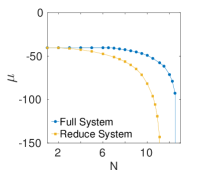
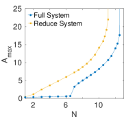
Figure 7: Comparison of the curves for the chemical potential, $\mu(N)$, and amplitude, $A_{\max}(N)$, obtained in the full and reduced systems (rhombuses and triangles, respectively). Other fixed parameters are the same as in Fig. 1.

(a)	(b)

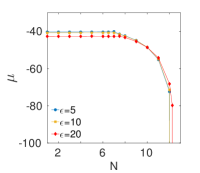
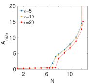
Figure 8: Chemical potential, $\mu$, and maximum amplitude, $A_{\max}$, as a function of $N$ for different values of the Zeeman-splitting strength, $\varepsilon$. Other fixed parameters are the same as in Fig. 1.

Finally, taking into account the Zeeman splitting, represented by coefficient $\varepsilon$ in Eqs. (1), Fig. 8 shows its effect on the MM’s chemical potential and amplitude. While the effect is not dramatic, it somewhat additionally stabilizes the MM, making its chemical potential more negative with the increase of $\varepsilon$. In addition to that, Fig. 8(b) shows that the increase of $\varepsilon$ increases the threshold value $N_{\min}$ above which the MMs exist.

4 Moving solitons and collisions between them

4.1 Soliton mobility

The SOC terms break the Galilean invariance of the underlying equations, therefore generation of the moving solitons from quiescent ones is a nontrivial problem for SOC systems [49]. To create such modes, moving in the $y$ direction, in direct simulations, we apply a kick to the originally quiescent MM soliton, multiplying both components of the spinor wave function by an exponential factor, $\exp(iky)$. Figure 9 shows two examples of the so generated spatiotemporal dynamics of the soliton’s component $|\Psi_{1}|$. Naturally, imparting larger momentum $k$ to the soliton gives rise to faster motion. Furthermore, Fig. 10 shows that the solitons move with an oscillating component in their velocity and amplitude. Solitons moving with higher velocities are found to be wider, and they demonstrate larger oscillations. This feature is a precursor of the destruction of solitons which are set in too fast motion, see below.

Alternatively, following work [49], solutions for solitons steadily moving at a given velocity $\mathbf{v}=(v_{x},v_{y})$ can be obtained from Eq. (1) rewritten in the reference frame moving with velocity $\mathbf{v}$:

$$i\frac{{\partial{\Psi_{1}}}}{{\partial t}}-i\left(\mathbf{v}\cdot\nabla\right)\Psi_{1}=-\frac{1}{2}{\nabla^{2}}{\Psi_{1}}+{\left|{{\Psi_{1}}}\right|^{4/3}}{\Psi_{1}}-\gamma{\left|{{\Psi_{2}}}\right|^{2}}{\Psi_{1}}+\lambda\left({\frac{{\partial{\Psi_{2}}}}{{\partial x}}-i\frac{{\partial{\Psi_{2}}}}{{\partial y}}}\right),$$

$$i\frac{{\partial{\Psi_{2}}}}{{\partial t}}-i\left(\mathbf{v}\cdot\nabla\right)\Psi_{2}=-\frac{1}{2}{\nabla^{2}}{\Psi_{2}}+{\left|{{\Psi_{2}}}\right|^{4/3}}{\Psi_{2}}-\gamma{\left|{{\Psi_{1}}}\right|^{2}}{\Psi_{2}}-\lambda\left({\frac{{\partial{\Psi_{1}}}}{{\partial x}}+i\frac{{\partial{\Psi_{1}}}}{{\partial y}}}\right).$$ (10)

Stable stationary MM solitons have been produced by the numerical solution of Eq. (10), for the velocity vector $\mathbf{v}=(0,v_{y})$ (moving solitons with $v_{x}\neq 0$ could not be found). Obviously, such solitons are moving ones, in terms of the laboratory reference frame. Note that the stationary version of Eqs. (10), produced by the substitution of ansatz (6), features the same symmetry which is evident in Eqs. (7) [57]:

$$U_{1,2}(x,y)=U_{2,1}\left(-x,y\right).$$ (11)

(a)	(b)

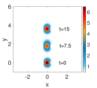
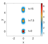
Figure 9: Contour plots of $|\Psi_{1}\left(x,y\right)|$ in the $\left(x,y\right)$ plane for a mixed-mode soliton, suddenly set in motion by kicks with $v_{y}=0.21$ (a) and $v_{y}=0.31$ (b). The evolution of the solitons is displayed at three moments of time, as indicated in the panels. Fixed parameters here are $\gamma=1$, $\varepsilon=0$, $\lambda=8$, and $N=10$.

(a)	(b)

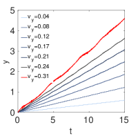
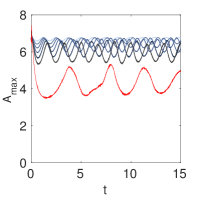
Figure 10: (a) The  coordinate of the position of the maximum density (center), and the amplitude of the kicked soliton, versus time. Fixed parameters are the same as in Fig. 9.

Figure 11 shows the amplitude of the steadily moving MM, produced by the solution of Eq. (10), as a function of $v_{y}$, at three different values of the SOC strength, $\lambda$. It is seen that the amplitude decreases with the growth of the velocity, but increases with the growth of $\lambda$. At the critical value of $v_{y}$, the amplitude abruptly vanishes, which implies nonexistence of MMs moving with velocities exceeding the critical value. In the binary-BEC system, SOC also prevents the existence of MM solitons at velocities exceeding a critical value [49], but the vanishing of the amplitude with the increase of $v_{y}$ is smoother than in the present case. On the other hand, the critical velocity increases with $\lambda$, showing that the solitons’ stability enhances for sharper solitons.

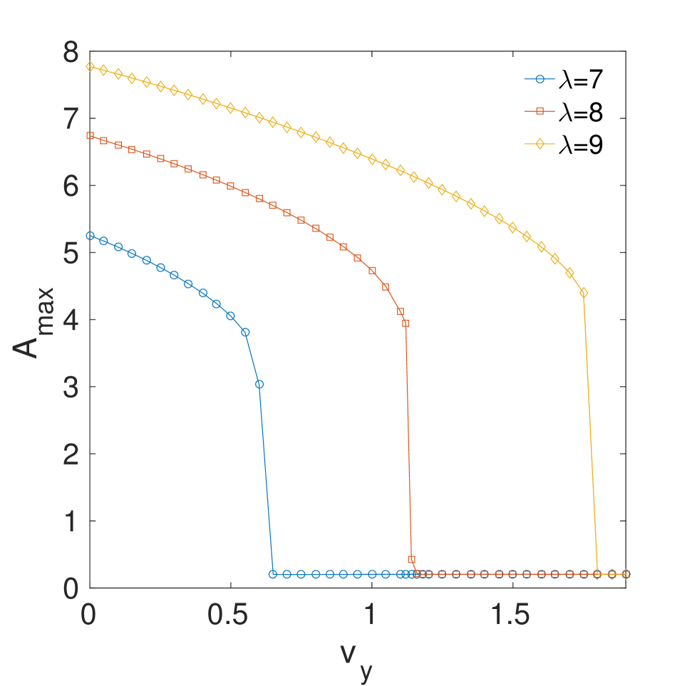
Figure 11: The amplitude of moving solitons, produced as stationary solutions of Eqs. (10), as a function of $v_{y}$. The moving solitons cease to exist when the amplitude falls to zero. Parameters are the same as in Fig. 9.

(a)	(b)
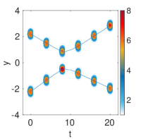
(c)	(d)

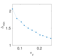
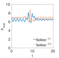
Figure 12: A typical example of elastic collisions between identical solitons moving in opposite directions is shown by means of contour plots of both component, $|\Psi_{1}|$ (a) and $|\Psi_{2}|$ (b), in the plane of $(x,y)$, at several moments of time, $t$, as a function of the $y$-position of the maximum amplitude and time. (c) The minimum separation between the bouncing solitons, $\Delta_{\min}$, as a function of the initial velocity, $\pm v_{y}$. The fixed parameters are $v_{y}=0.2$ and $N=20$, while the others are the same as in Fig. 9. (d) Amplitudes of the colliding solitons as functions of time, with “Soliton^(-)” and “Soliton⁽⁺⁾” referring to the solitons originally placed at $y<0$ and $y>0$, respectively.

(a)	(b)

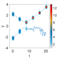
	(c)

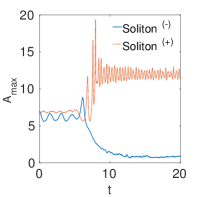
Figure 13: An inelastic collision leading to destruction of one soliton. Panels (a), (b), and (c) have the same meaning as (a), (b), and (d), respectively, in Fig. 12. The parameters are $v_{y}=0.27$, $N=20$, the others being the same as in Fig. 9.

4.2 Collisions between counterpropagating solitons

The availability of the moving solitons suggests to consider collisions between them. Solutions were initiated by taking a pair of solitons separated by distance $d$, kicked by factors $\exp(\pm i\mathbf{k}\cdot\mathbf{r})$. A typical picture, displayed in Fig. 12, demonstrates that the colliding solitons bounce back from each other, after reaching a minimal distance, $\Delta_{\min}$. This distance is shown in Fig. 12(c) as a function of the initial velocity, $\pm v_{y}$. The decrease of $\Delta_{\min}$ with the increase of $v_{y}$ is a natural result. Indeed, if the effective potential of the repulsion between the 2D solitons depends on the distance between them, $\Delta$, in the usual exponential form, $U_{\mathrm{rep}}\simeq U_{0}\exp\left(-\Delta/\Delta_{0}\right)$, with positive $U_{0}$ and $\Delta_{0}$ [83], the balance of the repulsive potential and the solitons’ kinetic energy (provided that it may be estimated as in the Galilean-invariant systems, $E_{\mathrm{kin}}\sim v_{y}^{2}$, predicts $\Delta_{\min}\sim\ln\left(1/v_{y}\right)$, for relatively small $v_{y}$.

The dependence of amplitudes of the colliding solitons on time, displayed in Fig. 12(d), shows that the initial kicks excite internal oscillations in the solitons [cf. Fig. 10)], as they break symmetry (11) of the stationary MMs, and the kick of opposite signs, $\pm k$, break it differently. Further, Fig. 12(c) demonstrates that the collision leads to the switch of inner oscillations between the two solitons.

In addition to elastic collisions shown in Fig. 12, the simulations reveal another outcome, in the form of partial destruction, as shown in Fig. 13: one soliton bounces back in a strongly excited state, while the other one (the soliton which featured conspicuous intrinsic excitation as the result of the initial kick) suffers destruction. Note that the amplitude (hence also the norm) of the surviving soliton essentially exceed their initial values, as it absorbs a large share of the norm from the destroyed soliton. For this reason, such an outcome of the collision may be categorized as partial merger of the colliding solitons.

Detailed study of collisions demonstrates additional outcomes (which can be observed, in particular, by varying the norm of the solitons), such as quasi-elastic passage of solitons through each other, excitation of strong inner oscillations, and destruction of both solitons. Complete results for collisions will be presented elsewhere.

5 Conclusion

The objective of this work is to construct stable self-trapped vortex-soliton complexes in the 2D model of the Fermi gas with two components, representing spin-up and down-polarized atomic states, linearly interacting through by the SOC (spin-orbit-coupling) terms of the Rashba type and contact nonlinear attraction, competing with the effective Pauli self-repulsion in each component, predicted by the density-functional theory for the binary Fermi gas. In addition to its physical significance, the model is interesting as it makes it possible to study the interplay of the linear SOC effect with competing self-repulsive and cross-attractive terms, which feature different powers of the nonlinearity. As a limit case, corresponding to the domination of the inter-component attraction, the system without the intrinsic repulsion was also considered, which corresponds to a binary bosonic gas as well. The systematic numerical analysis has produced a parameter region populated by stable two-component solitons of the MM (mixed-mode) type, while all the SV (semi-vortex) solitons are found to be unstable. The largest velocity up to which the solitons may travel in this system with the broken Galilean invariance has been identified too. Finally, we have briefly addressed collisions between solitons moving in opposite directions, demonstrating various outcomes of the collisions, such as quasi-elastic rebound of the solitons from each other, and destruction of one of them.

The analysis reported in this work can be extended by including a combination of the Rashba and Dresselhaus types of SOC (cf. the analysis performed in Ref. [53] for 2D solitons in binary BEC). Another interesting possibility is to consider the limit case of “heavy atoms”, i.e., negligible kinetic-energy terms in Eq. (1). As shown in terms of the binary bosonic gas under the action of SOC, in this case the dispersion law (4) is replaced by one which features a gap, $\mu=\pm\sqrt{\varepsilon^{2}+\lambda^{2}k^{2}}$, that can be populated by gap solitons [84]. The consideration of the respective model for the binary Fermi gas will be reported elsewhere. Lastly, a challenging possibility is to extend the work for 3D settings, cf. the prediction of metastable solitons supported by SOC in the 3D bosonic gas [59].

References

- [1] Giorgini S, Pitaevskii LP, Stringari S. Rev Mod Phys 2008;80:1215.
- [2] Bloch I, Dalibard J, Zwerger W. Rev Mod Phys 2008;80:885.
- [3] Baumann K, Guerlin C, Brennecke F, Esslinger T. Nature 2010;464:130.
- [4] Zipkes C, Palzer S, Sias C Köhl M. Nature 2010;464:388.
- [5] Perron JK, Kimball MO, Mooney KP, Gasparini FM. Nature Physics 2010;6:499.
- [6] Lieb EH, Liniger W. Phys Rev 1963;130:1605.
- [7] Lieb EH. Phys Rev 1963;130:1616.
- [8] Gaudin M. Phys Lett A 1967;24:55.
- [9] Yang CN. Phys Rev Lett 1967;19:1312.
- [10] Fuchs JN, Recati A, Zwerger W. Phys Rev Lett 2004;93:090408.
- [11] Hu H, Liu XJ, Drummond PD. Phys Rev Lett 2007;98:070403.
- [12] Giraud S, Combescot R. Phys Rev A 2009;79:043615.
- [13] Blume D, Rakshit D. Phys Rev E 2009;80:013601.
- [14] Pitaevskii LP, Stringari A. Bose-Einstein Condensation Clarendon Press: Oxford; 2003.
- [15] Salasnich L. J Math Phys 2000;41:8016.
- [16] Salasnich L, Pozzi B, Parola A, Reatto L. J Phys B 2000;33:3943.
- [17] Das KK. Phys Rev Lett 2003;90:170403.
- [18] Adhikari SK. Phys Rev A 2004;70:043617.
- [19] Adhikari SK. Phys Rev A 2005;72:053608.
- [20] Adhikari SK. Phys Rev A 2006;73:043619.
- [21] Adhikari SK, Malomed BA. Phys Rev A 2006;74:053620.
- [22] Salasnich L, Adhikari SK, Toigo F. Phys Rev A 2007;75:023616.
- [23] Adhikari SK. Phys Rev A 2007;76:053609.
- [24] Adhikari SK, Salasnich L. Phys Rev A 2007;76:023612.
- [25] Adhikari SK, Salasnich L. Phys Rev A 2008;78:043616.
- [26] Adhikari SK, Salasnich L. New J Phys 2009;11:023011.
- [27] Adhikari SK, Lu H, Pu H. Phys Rev A 2009;80:063607.
- [28] Anderson BP, Haljan PC, Regal CA, Feder DL, Collins LA, Clark CW, Cornell EA. Phys Rev Lett 2001;86:2926.
- [29] Ginsberg NS, Br J, Hau LV. Phys Rev Lett 2005;94:040403.
- [30] Shomroni I, Lahoud E, Levy S, Steinhauer J. Nature Physics 2009;5:193.
- [31] Dutton Z, Budde M, Slowe C, Hau LV. Science 2001;293:663.
- [32] Chang JJ, Engels P, Hoefer MA. Phys Rev Lett 2008;101:170404.
- [33] Ott H, Fortägh J, Kraft S, Günther A, Komma D, Zimmermann C. Phys Rev Lett 2003;91:040402.
- [34] Yefsah T, Sommer AT, Ku MJH, Cheuk LW, Ji WJ, Bakr WS, Zwierlein MW. Phys Rev A 2007;75:011603.
- [35] Antezza M, Dalfovo F, Pitaevskii LP, Stringari S. Phys Rev A 2007;76:043610.
- [36] Adhikari SK, Salasnich L. Phys Rev A 2008;78:043616.
- [37] Díaz P, Laroze D, Malomed BA, Schmidt I. J Phys B At Mol Opt Phys 2012;45:145304.
- [38] Yefsah T, Sommer AT, Ku MJH, Cheuk LW, Ji WJ, Bakr WS, Zwierlein MW. Nature 2013;429:426.
- [39] Jie JY, Dou FQ, Duan WS. Eur Phys J 2014;87:271.
- [40] Díaz P, Laroze D, Malomed BA. J Phys B At Mol Opt Phys 2015;48:075301.
- [41] Lombardi G, Van Alphen W, Klimin SN. J Tempere Phys Rev A 2017;96:033609.
- [42] Shang C, Zheng YL, Malomed BA. Phys Rev A 2018;97:043602.
- [43] Bergé L. Phys Rep 1998;303:259.
- [44] Fibich G. The Nonlinear Schrödinger Equation: Singular Solutions:Optical Collapse Springer: Heidelberg; 2015.
- [45] Mardonov SH, Ya Sherman E, Muga JG, Wang HW, Ban Y, Chen X. Phys Rev A 2015;91:043604.
- [46] Malomed BA, Mihalache D, Wise F, Torner L. J Optics B Quant Semicl Opt 2005;7:R53; J Phys B At Mol Opt Phys 2016;49:170502.
- [47] Malomed BA. Eur Phys J Special Topics 2016;225:2507.
- [48] Mihalache D. Rom Rep Phys 2017;69:403.
- [49] Sakaguchi H, Li B, Malomed BA. Phys Rev E 2014;89:032920.
- [50] Lobanov VE, Kartashov YV, Konotop VV. Phys Rev Lett 2014;112:180403.
- [51] Salasnich L, Cardoso WB, Malomed BA. Phys Rev A 2014;90:033629.
- [52] Xu Y, Zhang Y, Zhang C. Phys Rev A 2015;92:013633.
- [53] Sakaguchi H, Ya Sherman E, Malomed BA. Phys Rev E 2016;94:032202.
- [54] Gautam S, Adhikari SK. Phys Rev A 2017;95:013608.
- [55] Li Y, Luo Z, Liu Y, Chen Z, Huang C, Fu S, Tan H. Malomed BA. New J Phys 2017;19:113043.
- [56] Chen G, Liu Y, Wang H. Commun Nonlinear Sci Numer Simulat 2017;48:318.
- [57] Sakaguchi H, Li B, Ya Sherman E, Malomed BA. Romanian Rep Phys 2018;70:502 .
- [58] Sakaguchi H, Malomed BA. Phys Rev A 2018;97:013607.
- [59] Zhang YC, Zhou ZW, Malomed BA, Pu H. Phys Rev Lett 2015;115:253902.
- [60] Malomed BA. EPL 2018; 122:36001.
- [61] Lin YJ, Jiménez-García K, Spielman IB. Nature 2011;471:83.
- [62] Campbell DL, Juzeliūnas G, Spielman IB. Phys Rev A 2011;84:025602.
- [63] Zhang Y, Mao L, Zhang C. Phys Rev Lett 2012;108:035302.
- [64] Anderson BM, Juzeliūnas G, Galitski VM, Spielman IB. Phys Rev Lett 2012;108:235301.
- [65] Wu Z, Zhang L, Sun W, Xu XT, Wang BZ, Ji SC, Deng Y, Chen S, Liu XJ, Pan JW. Science 2016;354:83.
- [66] Li Y, Luo Z, Liu Y, Chen Z, Huang C, Fu S, Tan H, Malomed BA. New J Phys 2017;19:113043.
- [67] Zhou K, Zhang Z. Phys Rev Lett 2012;108:025301.
- [68] Chen G, Gong M, Zhang C. Phys Rev A 2012;85:013601 .
- [69] Spielman IB. Ann Rev Cold At Mol 2012;1:145 .
- [70] Galitski VI, Spielman B. Nature 2013;494:49.
- [71] Goldman N, Juzeliūnas G, Öhberg P Spielman B. Rep Progr Phys 2014;77:126401.
- [72] Zhai H. Rep Progr Phys 2015;78:026001.
- [73] Wu Z, Zhang L, Sun W, Xu XT, Wang BZ, Ji SC, Deng Y, Chen S, Liu XJ, Pan JW. Science 2016;354:83.
- [74] Huang L, Meng Z, Wang P, Peng P, Zhang SL, Chen L, Li D, Zhou Q, Zhang J. Nature Phys 2016;12:540.
- [75] Bychkov YA, Rashba EI. J Phys C 1984;17:6039.
- [76] Rashba EI, Sherman EI. Phys Lett 1988;129:175.
- [77] Regal AA, Greiner M, Jin DS. Phys Rev Lett 2004;92:040403.
- [78] Bloch I, Dalibard J, Zwerger W. Rev Mod Phys 2008;80:885.
- [79] Sakaguchi H, Malomed BA. New J Phys 2016;18:105005.
- [80] Chiofalo ML, Succi SM, Tosi P. Phys Rev E 2000;62:7438.
- [81] Feder DL, Pindzola MS, Collins LA, Schneider BI, Clark CW. Phys Rev A 2000;62:053606.
- [82] Vakhitov M, Kolokolov A. Radiophys Quant Electron 1973;16:783.
- [83] Malomed BA. Phys Rev E 1998;58:7928.
- [84] Sakaguchi H, Malomed BA. Phys Rev A 2018;97:013607.