Resource-efficient analyzer of Bell and Greenberger-Horne-Zeilinger states of multiphoton systems

Abstract

We propose a resource-efficient error-rejecting entangled-state analyzer for polarization-encoded multiphoton systems. Our analyzer is based on two single-photon quantum-nondemolition detectors, where each of them is implemented with a four-level emitter (e.g., a quantum dot) coupled to a one-dimensional system (such as a micropillar cavity or a photonic nanocrystal waveguide). The analyzer works in a passive way and can completely distinguish $2^{n}$ Greenberger-Horne-Zeilinger (GHZ) states of $n$ photons without using any active operation or fast switching. The efficiency and fidelity of the GHZ-state analysis can, in principle, be close to unity, when an ideal single-photon scattering condition is fulfilled. For a nonideal scattering, which typically reduces the fidelity of a GHZ-state analysis, we introduce a passively error-rejecting circuit to enable a near-perfect fidelity at the expense of a slight decrease of its efficiency. Furthermore, the protocol can be directly used to perform a two-photon Bell-state analysis. This passive, resource-efficient, and error-rejecting protocol can, therefore, be useful for practical quantum networks.

I Introduction

Quantum entanglement is a fascinating phenomenon in quantum physics Horodecki et al. (2009), which provides a promising platform for various quantum technologies, including quantum communication networks Kimble (2008). Sharing quantum entanglement among distant network nodes is a prerequisite for many practical applications Cirac et al. (1999); Lim et al. (2005); Jiang et al. (2007); Qin et al. (2017); Lo et al. (2014); Bennett et al. (1993); Pirandola et al. (2015). There are two main obstacles for practical applications of multipartite quantum entanglement, i.e., entanglement generation over desired nodes and entanglement analysis within a local node. Usually, it is difficult to distribute local entanglement over spatially-separated nodes due to channel high losses Gisin et al. (2002). An efficient method to overcome channel noise uses quantum repeaters Dür et al. (1999); Jiang et al. (2009); Wang et al. (2012a); Munro et al. (2012), which are based on entanglement purification Bennett et al. (1996); Deutsch et al. (1996); Sheng et al. (2008); Sheng and Deng (2010) and quantum swapping Żukowski et al. (1993); Chen and She (2011); Hu and Rarity (2011); Chen et al. (2013); Su et al. (2016). By applying a proper entanglement analysis and local operations, one can complete an entanglement-purification protocol to distill some entanglement of a higher fidelity, and enlarge the distance of an entangled channel through quantum swapping. In addition to entanglement purification and entanglement swapping, Bell-state analysis is crucial, e.g., for quantum teleportation Bennett et al. (1993); Pirandola et al. (2015), quantum secure direct communication Long and Liu (2002); Deng et al. (2003); Hu et al. (2016); Zhang et al. (2017), and quantum dense coding Pan et al. (2012). It plays an essential role in various entanglement-based quantum information processing protocols Lo et al. (2014); Bennett et al. (1993); Pirandola et al. (2015); Long and Liu (2002); Deng et al. (2003); Hu et al. (2016); Zhang et al. (2017); Gisin et al. (2002); Dür et al. (1999); Jiang et al. (2009); Wang et al. (2012a); Munro et al. (2012); Bennett et al. (1996); Deutsch et al. (1996); Sheng et al. (2008); Sheng and Deng (2010); Żukowski et al. (1993); Chen and She (2011); Hu and Rarity (2011); Chen et al. (2013); Su et al. (2016); Pan et al. (2012).

Multipartite entanglement, compared to two-particle entanglement, is more powerful to reveal the nonlocality of quantum physics Horodecki et al. (2009); Pan et al. (2012); Deng et al. (2017); Tashima et al. (2016). The Greenberger-Horne-Zeilinger (GHZ) states enable more refined demonstrations of quantum nonlocality, and can be used to build more complex quantum networks involving many nodes Hillery et al. (1999); Schauer et al. (2010); Farouk et al. (2018); Dong et al. (2017) and to perform, i.e., conference-key agreement Ribeiro et al. (2018). Furthermore, GHZ states enable efficient methods for large-scale cluster-state generation for measurement-based quantum computing Briegel et al. (2009); Tanamoto et al. (2006); You et al. (2007); Tanamoto et al. (2009); Economou et al. (2010); Gimeno-Segovia et al. (2015); Li et al. (2015), and also provide a useful basis for quantum metrology Giovannetti et al. (2004); Dür et al. (2014). The generation and analysis of $n$-photon GHZ entanglement are highly demanding. To date, various efficient methods to generate the GHZ entanglement have been developed for different physical systems Wei et al. (2006); Wang et al. (2010); Macrì et al. (2018); Monz et al. (2011); Kaufmann et al. (2017); Yu et al. (2007); Zheng et al. (2012); Reiter et al. (2016); Shao et al. (2017). In photonic systems, an eight-photon GHZ state and a three-photon high-dimensional GHZ state have been experimentally demonstrated Huang et al. (2011); Yao et al. (2012); Malik et al. (2016); Krenn et al. (2016) by performing quantum fusion combined with post-selection operations and quantum interference Pan et al. (2012); Krenn et al. (2017); Bergamasco et al. (2017). By using a time delay, a resource-efficient method was proposed and demonstrated Megidish et al. (2012) for generating a six-photon GHZ state. It is possible to generate photonic GHZ states or other multipartite-entangled states in a deterministic way based on nonlinear processes Duan and Kimble (2004); Li et al. (2011); Hao et al. (2015); Reiserer et al. (2014); Reiserer and Rempe (2015). However, it is difficult to distribute such a GHZ state efficiently to distant nodes, due to the inefficiency of the GHZ sources and high losses during transmission Gisin et al. (2002); Perseguers et al. (2013). One possible solution is to establish entanglement pairs between a center node and distant nodes in parallel Dür et al. (1999); Jiang et al. (2009); Wang et al. (2012a); Munro et al. (2012), and then to perform quantum swapping with a GHZ-state analysis in the center node Bose et al. (1998); Lu et al. (2009).

In 1998, Pan and Zeilinger proposed, to our knowledge, the first practical GHZ-state analysis with linear-optical elements Pan and Zeilinger (1998). Their proposal can identify two of n-photon GHZ states by post-selection operations. In principle, one can constitute a nearly deterministic n-photon GHZ-state analysis with linear optics, when massive ancillary photons are used Kok et al. (2007). However, according to the Cansamiglia-Lütkenhaus no-go theorem Calsamiglia and Lütkenhaus (2001), perfect and deterministic Bell-state analysis on two polarization-encoded qubits is impossible by using only linear-optical elements (in addition to photodetectors) and auxiliary modes in the vacuum state. By taking into account nonlinear processes, a complete GHZ-state analysis for photonic systems becomes possible Qian et al. (2005); Xia et al. (2014), and can achieve perfect efficiency and fidelity for an ideal process. Moreover, a complete entangled-state analysis for hyperentangled or redundantly encoded photon pairs is possible Zhou and Sheng (2015); Sheng et al. (2010); Ren et al. (2012); Wang et al. (2012b); Liu and Zhang (2015); Wang et al. (2016a). The existing GHZ-state analyses typically require active operations and/or fast switching, and always require more quantum resources when the photon number of a given GHZ state increases. Furthermore, the fidelity of the Bell-state or GHZ-state analyses significantly depends on the nonlinearity strength of realistic nonlinear processes Reiserer and Rempe (2015). A deviation from an ideal nonlinear process leads to errors and, thus, reduces the fidelity. These disadvantages significantly limit applications of a GHZ-state analysis for practical quantum networks.

Here we propose a resource-efficient passive protocol of a multiphoton GHZ-state analysis using only two single-photon nondestructive [quantum nondemolition (QND)] detectors, three standard (destructive) single-photon detectors, and some linear-optical elements. The GHZ-state analysis circuit is universal, and can completely distinguish $2^{n}$ GHZ states with different photon numbers $n$, according to the measurement results of single-photon nondestructive and destructive detectors. The circuit works in a passive way as the Pan-Zeilinger GHZ-state analyzer does Pan and Zeilinger (1998). During the entangled-state analysis, there are neither active operations on ancillary atoms nor adaptive switching of photons Witthaut et al. (2012). The efficiency of our GHZ-state analysis can, in principle, be equal to one. Moreover, our protocol has no requisite for direct Hong-Ou-Mandel interference which requires simultaneous operations on two individual photons. Thus, we can significantly simplify the process of GHZ-state analysis and, subsequently, the structure of multinode quantum networks. Furthermore, the detrimental effect on the fidelity, introduced by a nonideal scattering process, can be eliminated passively at the expense of a decrease of its efficiency. Therefore, our protocol is resource efficient and passive, and can be used to efficiently entangle distant nodes in complex quantum networks.

The paper is organized as follows: A quantum interface between a single photon and a single quantum dot (QD) is introduced briefly in Sec. II for performing QND measurements on linearly polarized photons. In Sec. III, a passive GHZ-state analysis circuit is presented. In Sec. IV, a method to efficiently generate entanglement among distant nodes is described. Subsequently, the performance of the circuit, with state-of-the-art experimental parameters, is discussed in Sec. V. We conclude with brief discussion and conclusions in Secs. VI and VII. Moreover, Appendixes A and B present the two simplest examples of our method for the analysis of two-photon Bell states and three-photon GHZ states.

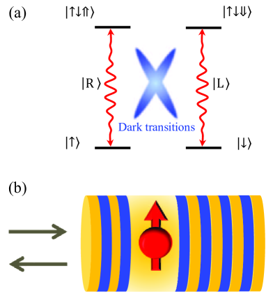
Figure 1: Proposal of quantum-nondemolition detection based on spin-dependent transitions for the negatively charged exciton $X^{-}$. (a) Relative-level structure and optical transition of a singly charged quantum dot (QD); (b) a QD coupled to an optical micropillar cavity. Here, $|\!\uparrow\rangle$ ($|\!\downarrow\rangle$) denotes the electron spin state with $J_{z}$ equal to 1/2 ($-$1/2), and $|\!\!\uparrow\downarrow\Uparrow\rangle$ ($|\!\!\uparrow\downarrow\Downarrow\rangle$) denotes the trion state of $X^{-}$ with $J_{z}$ equal to 3/2 ($-$3/2). A photon in a right- (left-) circularly-polarized state $|R\rangle$ ($|L\rangle$) can only couple to the transition $|\!\uparrow\rangle\leftrightarrow|\!\uparrow\downarrow\Uparrow\rangle$ ($|\!\downarrow\rangle\leftrightarrow|\!\uparrow\downarrow\Downarrow\rangle$). Therefore, the cross transitions are forbidden by the quantum-optical selection rules.

II Single-photon QND detector

An efficient interface, between a single photon and a single emitter, constitutes a necessary building block for various kinds of quantum tasks, especially for long-distance or distributed quantum networks Kimble (2008); Reiserer and Rempe (2015). To begin with, we consider a process of single-photon scattering by a four-level emitter coupled to a one-dimensional system, such as a QD coupled to a micropillar cavity or a photonic nanocrystal waveguide Reithmaier et al. (2004); Arcari et al. (2014); Li et al. (2018); Lodahl et al. (2015); Hu et al. (2008a, b). A singly-charged self-assembled In(Ga)As QD has four energy levels Hu et al. (2008a, b); Warburton (2013): two ground states of $J_{z}=\pm 1/2$, denoted as $|\!\uparrow\rangle$ and $|\!\downarrow\rangle$, respectively; and two optically excited trion states $X^{-}$, consisting of two electrons and one hole, with $J_{z}=\pm 3/2$, denoted as $|\!\!\uparrow\downarrow\Uparrow\rangle$ and $|\!\!\uparrow\downarrow\Downarrow\rangle$, respectively. Here the quantization axis $z$ is along the growth direction of the QD and it is the same as the direction of the input photon. Therefore, there are two circularly-polarized dipole transmissions which are degenerated when the environment magnetic field is zero, as shown in Fig. 1. A right-circularly polarized photon $|R\rangle$ and a left-circularly polarized photon $|L\rangle$ can only couple to the transitions $|\!\uparrow\rangle\leftrightarrow|\!\uparrow\downarrow\Uparrow\rangle$ and $|\!\downarrow\rangle\leftrightarrow|\!\uparrow\downarrow\Downarrow\rangle$, respectively.

The single-photon scattering process of a QD-cavity unit is dependent on the state of the QD. There are two individual cases: (1) If an input photon does not match the circularly polarized transition of the QD, the photon excites the cavity mode that is orthogonal to the polarization transition of the QD, and it is reflected by a practically empty cavity with a loss probability caused by photon absorption and/or side leakage. (Hereafter, for brevity, we refer to the side leakage only, but we also mean other photon absorption losses.) However, (2) if an input photon matches a given transition of the QD, the photon interacts with the QD and is reflected by the cavity that couples to the QD. Therefore, a j-circularly polarized photon (where $j=$right or left) in the input mode $\hat{a}^{\dagger}_{\omega_{j},\text{in}}$ of frequency $\omega_{j}$, after it is scattered by a QD-cavity unit, evolves into an output mode $\hat{a}^{\dagger}_{\omega_{j},\text{out}}$ as follows Hu et al. (2008a, b); Lodahl et al. (2015); Warburton (2013):

$$\hat{a}^{\dagger}_{\omega_{j},\text{in}}|0,0,{\bar{s}}\rangle\;\rightarrow\;r_{0}\hat{a}^{\dagger}_{\omega_{j},\text{out}}|0,0,{\bar{s}}\rangle,$$

$$\hat{a}^{\dagger}_{\omega_{j},\text{in}}|0,0,s\rangle\;\rightarrow\;r_{1}\hat{a}^{\dagger}_{\omega_{j},\text{out}}|0,0,s\rangle,$$ (1)

where the state $|0,0,s\rangle$ ($|0,0,\bar{s}\rangle$) denotes that both input and output fields are in the vacuum state and the QD is in the state $|s\rangle$ ($|\bar{s}\rangle$) that couples (does not couple) to the input photon. Under the assumptions of both adiabatic evolution of the cavity field and negligible excitation of the QD, the state-dependent reflection amplitudes $r_{0}$ and $r_{1}$, corresponding, respectively, to the aforementioned cases (1) and (2), are given by Hu et al. (2008a, b); Lodahl et al. (2015); Warburton (2013):

$$r_{0}(\omega) = 1-\frac{{\kappa}}{i(\omega_{c}\!-\!\omega)\!+\!\frac{\kappa}{2}\!+\!\frac{\kappa_{s}}{2}},$$

$$r_{1}(\omega) = 1-\frac{\kappa f}{\!\!\!\left[i(\omega_{c}\!-\!\omega)\!+\!\frac{\kappa}{2}\!+\!\frac{\kappa_{s}}{2}\right]\!f+\!g^{2}},$$ (2)

where the auxiliary function $f$ is given by $f=i(\omega_{X^{-}}-\omega)+\frac{\gamma}{2}$. Here $\omega_{X^{-}}$ is the transmission frequency of the QD and $\omega_{c}$ is the resonant frequency of the cavity. These frequencies can be tuned to be equal to $\omega_{X^{-}}=\omega_{c}$, for simplicity. Moreover, $\kappa$ describes a directional coupling between the cavity modes and the input and output modes; $g$ denotes the coupling between the QD and cavity; $\kappa_{s}$ represents the cavity side-leakage rate, and $\gamma$ is the trion decay rate. These formulas for the reflection coefficients are valid in general for both weak and strong couplings O’Brien et al. (2016).

For ideal scattering in the strong-coupling regime with $\kappa_{s}\ll\kappa$ and $\gamma,\kappa\ll{}g$ (or in the high-cooperativity regime with $\kappa_{s}\ll\kappa$, $\gamma\ll{}g\ll\kappa$, and $\gamma\kappa\ll{}g^{2}$) O’Brien et al. (2016), an input photon, that is resonant with a QD transition, is deterministically reflected by the QD-cavity unit. A $\pi$-phase (zero-phase) shift is introduced to the hybrid system consisting of a photon and the QD with $r_{0}=-1$ for $g=0$ ($r_{1}=1$ for $\kappa\gamma\ll{}g^{2}$), if the photon decouples (couples) to a transition of the QD. When the QD is initialized to be in the superposition state $|\pm\rangle=(|\!\uparrow\rangle\pm|\!\downarrow\rangle)/\sqrt{2}$, an input photon in a linearly polarized state evolves as follows:

$$|H\rangle|\pm\rangle\rightarrow|V\rangle|\mp\rangle,$$

$$|V\rangle|\pm\rangle\rightarrow|H\rangle|\mp\rangle.$$ (3)

Equation (3) means that if a QD receives a single photon, then it receives the Pauli $\sigma_{x}$ unitary. On the one hand, if the QD does not receive any photon, then it does not change its state. Thus, if we can identify whether the QD receives the Pauli $\sigma_{x}$ unitary, then it works as a QND measurement for photons Witthaut and Sørensen (2010); Hu et al. (2008a); O’Brien et al. (2016); Reiserer et al. (2013). Furthermore, when the QD receives a photon, then it flips the polarization state of the photon simultaneously Li et al. (2012); Li and Deng (2016). We will show in Sec. V that the QND measurement can work faithfully with a limited efficiency for practical scattering, i.e., when $r_{1}(\omega)$ and $r_{0}(\omega)$ significantly deviate from their ideal values $\pm 1$.

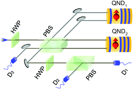
Figure 2: Schematics of the passive optical GHZ-state analyzer using single-photon QND detectors. Here PBS denotes a polarizing beam splitter, which transmits photons with horizontal polarization $|H\rangle$ and reflects those with vertical polarization $|V\rangle$. HWP represents a half-wave plate that performs the Hadamard transformation on photons passing it, i.e., $|H\rangle\rightarrow(|\!H\rangle+|\!V\rangle)/\sqrt{2}$ or $|V\rangle\rightarrow(|\!H\rangle-|\!V\rangle)/\sqrt{2}$. QND detection completes a nondestructive measurement on single photons, and D_i ($i=1,2,3$) is an ordinary (destructive) single-photon detector.

III Passive GHZ-state analyzer

III.1 The setup

So far, we have described a QND detection of linearly polarized single photons. In this section, we describe how to incorporate a QND detector into the setup for the passive optical GHZ-state analysis, as shown in Fig. 2. The setup is composed of two half-wave plates (HWPs), two polarizing beam splitters (PBSs), two single-photon QND detectors in the state $|+\rangle_{1}|+\rangle_{2}$, and several standard (destructive) single-photon detectors. The HWP is tuned to perform the Hadamard transformation on photons passing it, i.e., $|H\rangle\rightarrow(|\!H\rangle+|\!V\rangle)/\sqrt{2}$ or $|V\rangle\rightarrow(|\!H\rangle-|\!V\rangle)/\sqrt{2}$. The PBS transmits linearly-polarized photons in the state $|H\rangle$ and reflects photons in the state $|V\rangle$. The single-photon QND and standard detectors complete the photon on-off measurements in nondestructive and destructive ways, respectively.

III.2 GHZ states

For $n$-photon polarization-encoded GHZ states, the simplest two can be expressed as Pan et al. (2012):

$$|\text{GHZ}_{00...0}\rangle = \frac{1}{\sqrt{2}}\left(|H\rangle^{\otimes{}n}+|V\rangle^{\otimes{}n}\right),$$

$$|\text{GHZ}_{00...1}\rangle = \frac{1}{\sqrt{2}}\left(|H\rangle^{\otimes{}n}-|V\rangle^{\otimes{}n}\right),$$ (4)

where the last ($n$th) bit in the subscript of $|\text{GHZ}_{00...n}\rangle$ refers to the phase ($\pm$). If a photon is determined in the state $|H\rangle$ or $|V\rangle$, the remaining $(n-1)$ photons collapse into the same polarization. To constitute a complete basis for the $n$-photon system, one should take the remaining $(2^{n}-2)$ orthogonal basis states into consideration,

$$|\text{GHZ}_{i_{1}i_{2}...i_{n}}\rangle = \bigotimes_{j=1}^{n-1}\sigma^{i_{j}}_{x_{j}}\otimes\sigma^{i_{n}}_{z_{n}}|\text{GHZ}_{00...0}\rangle$$ (5)

$$= i\sigma^{i_{n}}_{y_{n}}\bigotimes_{j=1}^{n}\sigma^{i_{j}}_{x_{j}}|\text{GHZ}_{00...0}\rangle,$$

which can be generated from $|\text{GHZ}_{00...0}\rangle$ by performing a single-photon rotation on each photon, and

$$\bigotimes_{j=1}^{n}\sigma^{i_{j}}_{x_{j}}=\sigma_{x_{1}}^{i_{1}}\otimes\sigma_{x_{2}}^{i_{2}}\otimes...\otimes\sigma^{i_{n}}_{x_{n}}.$$

Here, the superscripts $i_{1}$, $i_{2}$, …, $i_{n}$ $\in\{0,1\}$, the Pauli operators $\sigma_{x_{j}}=|H\rangle_{j}\langle V|+|V\rangle_{j}\langle H|$ perform a polarization flip on the $j$th photon with $j=1,2,...,n$; $\sigma_{y_{n}}=-i(|H\rangle_{n}\langle V|-|V\rangle_{n}\langle{}H|$); $\sigma_{z_{n}}=|H\rangle_{n}\langle H|-|V\rangle_{n}\langle{}V|$ performs a phase flip on the $n$th photon; and the relative phase between the two components of Eq. (5) is determined by $i_{n}$; i.e., $i_{n}=0$ ($i_{n}=1$) leads to a relative phase of $0$ ($\pi$).

III.3 State transformations for the GHZ-state analysis

Now we focus on completely distinguishing the aforementioned $2^{n}$ GHZ states, which is of vital importance for multiuser quantum networks Pan and Zeilinger (1998); Lu et al. (2009); Bose et al. (1998). According to stabilizer theory Gottesman (1996); Tóth and Gühne (2005); Schmid et al. (2008); Greganti et al. (2015), the $n$-photon state $|\text{GHZ}_{00...0}\rangle$, given in Eq. (4), is a stabilizer state that can be uniquely defined by $n$ stabilizing operators $S_{k}$,

$$S_{k}=\left\{\begin{array}[]{ll}\sigma_{x_{1}}\otimes\sigma_{x_{2}}\otimes...\otimes\sigma_{x_{n}},&\hbox{$k=1$;}\\ \sigma_{z_{k-1}}\otimes\sigma_{z_{k}},&\hbox{$k=2,3,...,n.$}\end{array}\right.$$ (8)

Here the operators $\sigma_{z_{k}}$ perform a phase flip on the $k$th photon with $k=1,2,...,$ and $n$; there is an implicit identity $I^{\otimes(n-2)}$ acting on the remaining photons that is suppressed in $S_{k\geq 2}$ for simplicity.

The set of operators $S_{1}$, $S_{2}$, …, $S_{n}$ forms a complete set of commuting observables; the $2^{n}$ GHZ states are common eigenvectors of all $S_{k}$’s with different eigenvalues Tóth and Gühne (2005), i.e., $|\text{GHZ}_{00...0}\rangle$ gives an eigenvalue $+1$ for all $S_{k}$’s. Therefore, we can measure the stabilizing operators $S_{k}$’s to completely discriminate $2^{n}$ GHZ states of an $n$-photon system.

Here the $n$-photon observable $S_{1}$ corresponds to the measurement of the relative phase between the two terms in a GHZ state and can be nondestructively measured by using two QND detectors introduced in Sec. II; $S_{k\geq 2}$ corresponds to parity detection on the pair of $(k-1)$th and $k$th photons and is measured with direct polarization measurements on each photon scattered by the QND detectors. To explain in detail our GHZ-state analysis, we use the ket notation instead of the stabilizer codes, since the stabilizer states change during the analysis.

For clarity, we divide this GHZ-state analysis into several steps. Let us suppose that there is a spatial separation between each two optical elements such that all photons can pass a given optical element before entering another element. Note this requirement is not necessary, and we will demonstrate, in the next section, that our proposal also works when each photon is passing one by one from the input port to the output port and is measured by a single-photon destructive detector.

After passing $n$ photons though the HWP, the Hadamard transformation is performed on each photon, and the $2^{n}$ GHZ states are changed into superposition states of $2^{n-1}$ (out of $2^{n}$ possible) product states, each with an even (odd) number of $V$-polarized photons for $|\text{GHZ}_{i_{1}i_{2}...i_{n-1}0}\rangle$ ($|\text{GHZ}_{i_{1}i_{2}...i_{n-1}1}\rangle$) . For instance, the states $|\text{GHZ}_{i_{1}i_{2}...i_{n-1}0}\rangle$ and $|\text{GHZ}_{i_{1}i_{2}...i_{n-1}1}\rangle$, after the Hadamard transformation of each photon, evolve into

$$|\varPsi_{1}\rangle = \frac{1}{\sqrt{2^{n-1}}}\sum_{m=0}^{[\frac{n}{2}]}\sqrt{C^{2m}_{n}}|G^{i_{1},...,i_{n-1}}_{2m}\rangle,$$

$$|\varPhi_{1}\rangle = \frac{1}{\sqrt{2^{n-1}}}\sum_{m=1}^{[\frac{n+1}{2}]}\sqrt{C^{2m-1}_{n}}|G^{i_{1},...,i_{n-1}}_{2m-1}\rangle,$$ (9)

respectively. Here $[x]$ is the integer value function that rounds the number $x$ down to the nearest integer; $C^{m}_{n}=\frac{n!}{m!(n-m)!}$ is the binomial coefficient; the state $|G^{i_{1},...,i_{n-1}}_{m}\rangle$ is an $n$-photon superposition state that contains $m$ $V$-polarized photons and $(n-m)$ $H$-polarized photons as follows:

$$|G^{i_{1},...,i_{n-1}}_{m}\rangle=\frac{Z}{\sqrt{C^{m}_{n}}}\sum_{\begin{subarray}{c}l_{1},...,l_{n}\in\{0,1\}\end{subarray}}{\delta_{m,m^{\prime}}}\bigotimes_{j=1}^{n}\sigma^{l_{j}}_{x_{j}}|H\rangle^{\otimes{}n},$$ (10)

where $m^{\prime}=\sum_{j=1}^{n}l_{j}$ and $\delta_{m,m^{\prime}}$ is the Kronecker delta. The phase of each component is determined by the operator $Z=\bigotimes_{j=1}^{n-1}\sigma^{i_{j}}_{z_{j}}$, which is simplified to an identity operator when analyzing $|\text{GHZ}_{00...0}\rangle$ and $|\text{GHZ}_{00...1}\rangle$.

III.4 Measurements for the GHZ-state analysis

As follows from the above analysis, the relative phase of $|\text{GHZ}_{i_{1}i_{2}...i_{n}}\rangle$, which is determined by $i_{n}$, can be read out by measuring the number of $V$-polarized photons in the even-odd basis after applying the Hadamard transformation to $|\text{GHZ}_{i_{1}i_{2}...i_{n}}\rangle$. This measurement can be completed by a setup consisting of a PBS and two QD-cavity units (referred to as QND detectors). As demonstrated in Sec. II, a linearly polarized photon, after being scattered by a QND detector, changes its polarization state into an orthogonal state and flips the state of the detector QD. After all photons are either transmitted or reflected by the first PBS, and scattered by the QND detectors, the hybrid states of the two QDs and the $n$ photons, corresponding to the states $|\text{GHZ}_{i_{1}i_{2}...i_{n-1}0}\rangle$ and $|\text{GHZ}_{i_{1}i_{2}...i_{n-1}1}\rangle$, evolve, respectively, into

$$|\varPsi_{2}^{e}\rangle = \bigotimes_{j=1}^{n}\sigma_{x_{j}}|\varPsi_{1}\rangle|+\rangle_{1}|+\rangle_{2},$$

$$|\varPhi_{2}^{e}\rangle = \bigotimes_{j=1}^{n}\sigma_{x_{j}}|\varPhi_{1}\rangle|-\rangle_{1}|-\rangle_{2},$$ (11)

if $n$ is even, and into

$$|\varPsi_{2}^{o}\rangle = \bigotimes_{j=1}^{n}\sigma_{x_{j}}|\varPsi_{1}\rangle|+\rangle_{1}|-\rangle_{2},$$

$$|\varPhi_{2}^{o}\rangle = \bigotimes_{j=1}^{n}\sigma_{x_{j}}|\varPhi_{1}\rangle|-\rangle_{1}|+\rangle_{2},$$ (12)

if $n$ is odd. The combined states of the two QDs in QND detectors are different, and can be used to deterministically distinguish $|\varPsi_{1}\rangle$ from $|\varPhi_{1}\rangle$ for both cases of even and odd $n$.

To make this point clearer, we continue our analysis to measure the parity of each photon pair $[k-1,k]$ for the case of an arbitrary even $n$. Now, photons in different polarization states combine again at the first PBS, which is followed by an HWP. The HWP completes the Hadamard transformation on each photon passing through it and evolves the photonic component of the hybrid states into its original GHZ state, up to a phase difference $\pi$. For the states $|\varPsi_{2}^{e}\rangle$ and $|\varPhi_{2}^{e}\rangle$, given in Eq. (11), they evolve into

$$|\varPsi_{3}\rangle = \pm|\text{GHZ}_{i_{1}i_{2}...i_{n-1}0}\rangle|+\rangle_{1}|+\rangle_{2},$$

$$|\varPhi_{3}\rangle = \pm|\text{GHZ}_{i_{1}i_{2}...i_{n-1}1}\rangle|-\rangle_{1}|-\rangle_{2}.$$ (13)

Here $|\text{GHZ}_{i_{1}i_{2}...i_{n-1}0}\rangle$ and $|\text{GHZ}_{i_{1}i_{2}...i_{n-1}1}\rangle$ are the $n$-photon GHZ states given in Eq. (5); their sign is determined by the summation of the first $(n-1)$ subscripts with $m^{\prime\prime}=\sum_{j=1}^{n-1}i_{j}$, i.e., “$+$” for even $m^{\prime\prime}$ and “$-$” for odd $m^{\prime\prime}$. Subsequently, a photon-polarization measurement setup, consisting of a PBS and two destructive single-photon detectors D₁ and D₂, is used to detect the polarization of each photon and then divides the measurement results according to the number of clicks of each detector, i.e., when $n$ $H$-polarized ($V$-polarized) photons are detected, the $n$ input photons are projected into either $|\text{GHZ}_{00...0}\rangle$ or $|\text{GHZ}_{00...1}\rangle$, which can be distinguished by detecting the state of the QD in each QND detector.

It is seen that there is neither active feedback nor fast switching operations involved in the entangled-state analysis. The setup works in a completely passive way, which is similar to that based on linear-optical elements and single-photon detectors. When $n=2$, the GHZ-state analysis setup enables a passive Bell-state analysis for two-photon systems, which are typically denoted as

$$|\phi^{\pm}\rangle = \frac{1}{\sqrt{2}}\left(|H\rangle|H\rangle\pm|V\rangle|V\rangle\right),$$

$$|\psi^{\pm}\rangle = \frac{1}{\sqrt{2}}\left(|H\rangle|V\rangle\pm|V\rangle|H\rangle\right).$$ (14)

Detailed analyses for $n=2$ and $3$ are presented in Appendixes A and B, respectively.

IV Efficient distant multipartite entanglement generation for quantum networks

In quantum multinode networks, multipartite entanglement among many nodes is useful for practical quantum communication or distributed quantum computation Deng et al. (2017); Pan et al. (2012). A direct method for sharing the GHZ entanglement among several distant nodes can be enabled by a faithful entanglement distribution after locally generating the GHZ entanglement. However, the efficiency of such a multipartite entanglement distribution significantly decreases with the increasing photon number involved in the GHZ entanglement Gisin et al. (2002). Furthermore, the experimental methods for generating multiphoton GHZ entanglement are still inefficient due to the limited experimental technologies. A significantly more efficient method for distant GHZ state generation can be achieved by entanglement swapping. In the following, we describe a scheme for the GHZ entanglement generation among three stationary qubits, and these stationary qubits can be atomic ensembles, nitrogen-vacancy (NV) centers, QDs, and other systems Buluta et al. (2011).

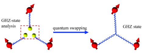
Figure 3: Schematics of nonlocal GHZ-state generation for multiparty quantum networks. Here a red circle with an arrow represents a stationary qubit, while a yellow circle represents a photon. Each wave line represents entanglement between the particles it connects.

Suppose there are three communicating nodes in a quantum network, say, Alice, Bob, and Charlie. An ancillary node (Eve) shares hybrid entanglement pairs with Alice, Bob, and Charlie, respectively, as follows Dür et al. (1999); Jiang et al. (2009); Wang et al. (2012a); Munro et al. (2012); Bennett et al. (1996); Deutsch et al. (1996); Sheng et al. (2008); Sheng and Deng (2010):

$$|\phi\rangle_{ji}=\frac{1}{\sqrt{2}}\left(|\!\uparrow\rangle_{j}|H\rangle_{i}+|\!\downarrow\rangle_{j}|V\rangle_{i}\right),$$ (15)

where the subscript $i$ (with $i=a,b,c$) represents the photons owned by Eve, and it is entangled with the $j$th QD (with $j=A,B,C$), which belongs to Alice, Bob, and Charlie, respectively, as shown in Fig. 3. The state $|\phi\rangle_{Aa}|\phi\rangle_{Bb}|\phi\rangle_{Cc}$ of the three hybrid entanglement pairs Aa, Bb, and Cc can be rewritten as

$$|\phi_{0}\rangle = \frac{1}{2\sqrt{2}}\sum_{i,j,k}|\text{GHZ}_{ijk}\rangle_{ABC}|\text{GHZ}_{ijk}\rangle_{abc}.$$ (16)

Here the subscripts $i$, $j$, $k\in\{0,1\}$, and the polarization-encoded GHZ states $|\text{GHZ}_{ijk}\rangle_{abc}$ are defined in Eq. (5) for $n=3$. The eight distant stationary GHZ states among Alice, Bob, and Charlie are of the following forms

$$|\text{GHZ}_{00k}\rangle_{ABC}\!=\!\frac{1}{\sqrt{2}}\big{[}|\!\uparrow\rangle_{A}|\!\uparrow\rangle_{B}|\!\uparrow\rangle_{C}\!+\!(\!-1)^{k}\!|\!\downarrow\rangle_{A}|\!\downarrow\rangle_{B}|\!\downarrow\rangle_{C}\big{]},$$

$$|\text{GHZ}_{10k}\rangle_{ABC}\!=\!\frac{1}{\sqrt{2}}\big{[}|\!\downarrow\rangle_{A}|\!\uparrow\rangle_{B}|\!\uparrow\rangle_{C}\!+\!(\!-1)^{k}\!|\!\uparrow\rangle_{A}|\!\downarrow\rangle_{B}|\!\downarrow\rangle_{C}\big{]},$$

$$|\text{GHZ}_{01k}\rangle_{ABC}\!=\!\frac{1}{\sqrt{2}}\big{[}|\!\uparrow\rangle_{A}|\!\downarrow\rangle_{B}|\!\uparrow\rangle_{C}\!+\!(\!-1)^{k}\!|\!\downarrow\rangle_{A}|\!\uparrow\rangle_{B}|\!\downarrow\rangle_{C}\big{]},$$

$$|\text{GHZ}_{11k}\rangle_{ABC}\!=\!\frac{1}{\sqrt{2}}\big{[}|\!\downarrow\rangle_{A}|\!\downarrow\rangle_{B}|\!\uparrow\rangle_{C}\!+\!(\!-1)^{k}\!|\!\uparrow\rangle_{A}|\!\uparrow\rangle_{B}|\!\downarrow\rangle_{C}\big{]},$$

with $k\in\{0,1\}$. These states constitute a complete basis for three-QD systems.

When the ancillary node Eve performs a quantum swapping operation with a three-photon polarization-encoded GHZ-state analysis, the states of the three stationary qubits, which belong to Alice, Bob, and Charlie, are projected into a deterministic GHZ state according to the analysis result of Eve. That is, we can, in principle, generate multipartite GHZ entanglement efficiently among distant stationary qubits with a perfect efficiency.

In Sec. III, we have described a particular pattern of the GHZ-state analysis with a preset time delay between each two optical elements. Now we demonstrate that the GHZ-state analysis also works for a time-delay free pattern, by performing the aforementioned quantum swapping as an example. Suppose both QDs in the QND detectors are initialized in the state $|+\rangle=(|\!\uparrow\rangle+|\!\downarrow\rangle)/\sqrt{2}$, and all the linear-optical elements perform the same operation as that described in Sec. III. The three photons from hybrid entanglement pairs Aa, Bb, and Cc, subsequently pass though the analysis setup independently, rather than transmitting them in a block pattern. After photon $a$ passing through the setup and being routed into two spatial modes that are ended with single-photon detectors, the hybrid system, consisting of three entanglement pairs and two QDs in the QND detectors, evolves into

$$|\phi_{1}\rangle = \frac{1}{2}\Big{[}|H\rangle_{a}\big{(}|+\rangle_{A}|+\rangle_{1}|-\rangle_{2}+|-\rangle_{A}|-\rangle_{1}|+\rangle_{2}\big{)}$$ (18)

$$-|V\rangle_{a}\big{(}|+\rangle_{A}|+\rangle_{1}|-\rangle_{2}-|-\rangle_{A}|-\rangle_{1}|+\rangle_{2}\big{)}\Big{]}$$

$$\otimes|\phi\rangle_{Bb}|\phi\rangle_{Cc}.$$

For clarity, we assume that the standard (destructive) single-photon detectors work nondestructively and a photon survives after a measurement on it, such that we can directly specify the state of the distant stationary qubits according to the state of the photon a. Subsequently, the photon b is input into the setup when the photon a has passed through the setup and lead to a click of either single-photon destructive detector D₁ or D₂. The hybrid system evolves into

$$|\phi_{2}\rangle\!\! = \!\!\frac{1}{2\sqrt{2}}\Big{[}\big{(}|\Phi^{+}\rangle_{AB}|+\rangle_{1}|+\rangle_{2}$$ (19)

$$\!\!+|\Phi^{-}\rangle_{AB}|-\rangle_{1}|-\rangle_{2}\big{)}|H\rangle_{a}|H\rangle_{b}-\big{(}|\Psi^{+}\rangle_{AB}|+\rangle_{1}|+\rangle_{2}$$

$$\!\!+|\Psi^{-}\rangle_{AB}|-\rangle_{1}|-\rangle_{2}\big{)}|H\rangle_{a}|V\rangle_{b}-\big{(}|\Psi^{+}\rangle_{AB}|+\rangle_{1}|+\rangle_{2}$$

$$\!\!-|\Psi^{-}\rangle_{AB}|-\rangle_{1}|-\rangle_{2}\big{)}|V\rangle_{a}|H\rangle_{b}+\big{(}|\Phi^{+}\rangle_{AB}|+\rangle_{1}|+\rangle_{2}$$

$$\!\!-|\Phi^{-}\rangle_{AB}|-\rangle_{1}|-\rangle_{2}\big{)}|V\rangle_{a}|V\rangle_{b}\Big{]}\otimes|\phi\rangle_{Cc},$$

where the four Bell states of the two QDs, belonging to Alice and Bob, are as follows:

$$|\Phi^{\pm}\rangle_{AB}=\frac{1}{\sqrt{2}}(|\!\uparrow\rangle_{A}|{\uparrow}\rangle_{B}\pm|\!\downarrow\rangle_{A}|\!\downarrow\rangle_{B}),$$

$$|\Psi^{\pm}\rangle_{AB}=\frac{1}{\sqrt{2}}(|\!\uparrow\rangle_{A}|\downarrow\rangle_{B}\pm|\!\downarrow\rangle_{A}|\!\uparrow\rangle_{B}),$$ (20)

Now, if Eve terminates the input of photon c and detects the two QDs of the QND detectors, the two distant QDs A and B are collapsed to one of the Bell states given in Eq. (20), according to the results of the QND detectors and the measurement on photons ab. That is, a deterministic quantum swapping operation can be completed between two hybrid entanglement pairs Aa and Bb by using the passive entanglement analysis setup.

If Eve inputs the photon $c$ into the analysis setup rather than terminating it with a measurement on the two QDs of the QND detectors, the state $|\phi_{2}\rangle$ of the hybrid system evolves into the final state

$$|\phi_{3}\rangle \!\!\!=\!\!\! \frac{1}{2\sqrt{2}}\!\sum_{ij}(\!-1)^{i+j}\!\Big{[}|\text{GHZ}_{ij0}\rangle_{ABC}|\text{GHZ}_{ij1}\rangle_{abc}|+\rangle_{1}|-\rangle_{2}$$ (21)

$$+|\text{GHZ}_{ij1}\rangle_{ABC}|\text{GHZ}_{ij0}\rangle_{abc}|-\rangle_{1}|+\rangle_{2}\Big{]},\;\;\;\;\;\;\;\;\;$$

with the subscripts $i,j\in\{0,1\}$. Three distant QDs A, B, and C are projected into a predetermined GHZ state, according to the results of the QND detectors and the single-photon destructive detectors, when Eve applies a polarization-encoded GHZ-state analysis on three photons of the hybrid entangled pairs. Therefore, in principle, the passive GHZ-state analysis works faithfully for both cases, i.e., the time-delay and time-delay-free cases, when an ideal single-photon QND detector is available.

V Performance of the passive GHZ-state analyser

V.1 Realistic photon scattering

A core element of the passive GHZ-state analysis is the QND detector for single photons. Here a unit consisting of a QD and a micropillar cavity enables such QND detection. In principle, the QND detector can perfectly distinguish two orthogonal polarization states $|H\rangle$ and $|V\rangle$ of a single photon with perfect efficiency. However, there are always some imperfections that introduce a deviation from ideal single-photon scattering Hu et al. (2008a, b); Li et al. (2018); Arcari et al. (2014); Lodahl et al. (2015), such as a finite single-photon bandwidth, a finite coupling $g$ between a QD and a cavity, and the nondirectional cavity side leakage $\kappa_{s}$, etc. This leads to realistic (nonideal) scattering for a linearly polarized photon. Thus, the hybrid system consisting of a linearly polarized single photon and a QD, evolves as follows:

$$|H\rangle|\pm\rangle \rightarrow \frac{1}{\sqrt{C_{N}}}[(r_{1}+r_{0})|H\rangle|\pm\rangle+(r_{1}-r_{0})|V\rangle|\mp\rangle],$$

$$|V\rangle|\pm\rangle \rightarrow \frac{1}{\sqrt{C_{N}}}[(r_{1}-r_{0})|H\rangle|\mp\rangle+(r_{1}+r_{0})|V\rangle|\pm\rangle],\;\;\;\;\;\;\;\;$$ (22)

where the parameters $r$ and $r_{0}$ are frequency-dependent reflection coefficients given in Eq. (2); $C_{N}=2(|r_{1}|^{2}+|r_{0}|^{2})$ is the normalized coefficient. After scattering, the state of the photon and the QD evolves in two ways independent of its initial state:

(1) It is flipped simultaneously with a probability $p_{1}=|r_{1}-r_{0}|^{2}/4$, which is the desired output and it can be simplified to perform an ideal QND detection, as given in Eq. (3), when ideal scattering with $r_{1}=1$ and $r_{0}=-1$ is achieved.

(2) The state of the photon and the QD are unchanged with the probability $p_{2}=|r_{1}+r_{0}|^{2}/4$, which leads to errors and results in an unfaithful QND detection for single photons.

Fortunately, this nonideal scattering does not affect the fidelity of the passive GHZ-state analysis, since the undesired scattering component is filtered out automatically by the PBS and only leads to an inconclusive result rather than infidelity result by a click of the single-photon destructive detector $D_{3}$.

V.2 Realistic analyzer efficiency

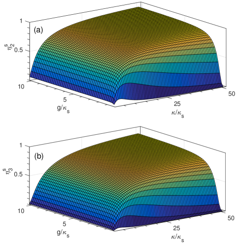
Figure 4: Average efficiencies (a) $\eta^{s}_{2}$ of the two-photon Bell-state analyzer and (b) $\eta^{s}_{3}$ of the three-photon GHZ-state analyzer versus the coupling strength $g/\kappa_{s}$ and the directional coupling rate of a cavity $\kappa/\kappa_{s}$ in units of the cavity side-leakage rate $\kappa_{s}$. These averages are calculated over all detunings of input photons, with the Gaussian spectrum given by Eq. (25) and $\sigma_{\omega}=\gamma$. The decay parameters are ($\kappa_{s},\gamma)=(30~{}\mu\,\text{eV},0.3~{}\mu\,\text{eV})$.

For ideal scattering, the analyzer efficiency approaches unity. Here, we evaluate the performance of a realistic analyzer for the general reflection amplitudes given in Eq. (2). Nonideal scattering in practical QND detection does not reduce the fidelity of an n-photon GHZ analysis. However, this realistic scattering decreases the efficiency $\tilde{\eta}^{s}_{n}$, which is defined as the probability that all photons are detected by a single-photon destructive detector, either $D_{1}$ or $D_{2}$. For monochromatic photons of a frequency $\omega$, the efficiency $\tilde{\eta}^{s}_{n}$ is defined as

$$\tilde{\eta}^{s}_{n}={\eta^{n}_{0}\eta^{n}_{1}(\omega)},$$ (23)

where $\eta_{0}$ is the efficiency of a single-photon detector $D_{i}$ and $\eta_{1}(\omega)$ is the error-free efficiency of a practical scattering with

$$\eta_{1}(\omega)=\left|\frac{r_{1}(\omega)-r_{0}(\omega)}{2}\right|^{2}.$$ (24)

The average efficiencies of the passive two-photon Bell-state and the three-photon GHZ-state analyzers are shown in Fig. 4 with decay parameters ($\kappa_{s},\gamma)=(30~{}\mu\,\text{eV},0.3~{}\mu\,\text{eV})$, which are adopted according to the QDs that are embedded in electrically controlled cavities around $4$ K Giesz et al. (2016); Somaschi et al. (2016). We plotted the average efficiencies $\eta^{s}_{2}$ and $\eta_{3}^{s}$ versus the coupling strength $g/\kappa_{s}$ and the directional coupling rate of the cavity $\kappa/\kappa_{s}$ for a given Gaussian single-photon pulse defined by the spectrum

$$f(\omega)=\frac{1}{\sqrt{\pi}\sigma_{\omega}}\exp\left[-\left(\frac{\omega-\omega_{c}}{\sigma_{\omega}}\right)^{2}\right],$$ (25)

where $\omega_{c}$ is the center frequency and $\sigma_{\omega}$ denotes the pulse bandwidth with $\omega_{c}=\omega_{X^{-}}$ and $\sigma_{\omega}=\gamma$. Here the average efficiencies are calculated in the frequency domain. The reflection coefficients appear as a frequency-dependent redistribution function that is proportional to $|r_{1}(\omega)-r_{0}(\omega)|^{2n}$ as follows DiVincenzo and Solgun (2013); Cohen and Mølmer (2018):

$$\eta^{s}_{n}=\int{}d\omega{}f(\omega)\eta^{n}_{0}\left|\frac{r_{1}(\omega)-r_{0}(\omega)}{2}\right|^{2n}.$$ (26)

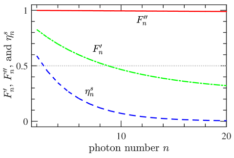
Figure 5: Average fidelities $F^{\prime}_{n}$, $F^{\prime\prime}_{n}$, and efficiency $\eta_{n}^{s}$ versus photon number $n$. Here $F^{\prime}_{n}\equiv F_{n}(T_{2}=10.9~{}{\rm ns})$ and $F^{\prime\prime}_{n}\equiv F_{n}(T_{2}=2~{}{\rm\mu{}s})$. These averages are calculated over all detunings of input photons, with the Gaussian spectrum given by Eq. (25) and $\sigma_{\omega}=2\gamma$. The decay parameters are ($\kappa_{s},\gamma)=(30~{}\mu\,\text{eV},0.3~{}\mu\,\text{eV})$, $g=\kappa_{s}$, and $\kappa=9\kappa_{s}$ with $C=10$. Meanwhile, the line of the fidelities at $1/2$ is shown for reference.

In general, the average efficiencies of the passive two-photon Bell-state and three-photon GHZ-state analyzers increase when the coupling $g/\kappa_{s}$ between a QD and a cavity is increased for a given directional coupling rate $\kappa/\kappa_{s}$. This is because the cooperativity

$$C=\frac{g^{2}}{\gamma\kappa_{T}}=\frac{g^{2}}{\gamma(\kappa+\kappa_{s})},$$ (27)

which is defined as an essential parameter quantifying the loss of an atom-cavity system, increases when we increase $g/\kappa_{s}$ and keep other parameters unchanged. For a given $g/\kappa_{s}$, the average efficiencies of these two analyzers first increase and then decrease when $\kappa/\kappa_{s}$ is increased, as shown in Fig. 4. This is mainly due to the competition between an increased ratio of $\kappa/\kappa_{s}$ and a decreased cooperativity $C$. Therefore, one can maximize the efficiencies by using cavities with a mediate $\kappa$, which can be achieved, e.g., by decreasing the number of the Bragg reflector of a micropillar cavity. For simplicity, we set the efficiency of a single-photon destructive detector as $\eta_{0}=1$.

For the two-photon Bell-state analyzer, its average efficiency $\eta^{s}_{2}=0.304$ for an experimental demonstrated coupling $g/\kappa_{s}=1$ and the directional coupling rate of a cavity, $\kappa/\kappa_{s}=3$, which corresponds to a cooperativity $C=25$. For the three-photon GHZ-state analyzer, one can obtain the average efficiency $\eta^{s}_{3}\simeq 0.168$ for the same systematic parameters. If $\kappa$ is increased to $\kappa/\kappa_{s}=19$ with a cooperativity $C=5$ Giesz et al. (2016), the average efficiencies are increased to $\eta^{s}_{2}\simeq 0.664$ and $\eta^{s}_{3}\simeq 0.541$, respectively. Note that the adiabatic condition is still satisfied in this case, since the photon bandwidth $\sigma_{\omega}=\gamma$ is much smaller than $2g^{2}/\kappa_{T}=2C\gamma$. The protocol works with a higher efficiency for analyzing photons with a narrower bandwidth. However, this, in turn, usually increases the time period of the scattering process, and, thus, decreases the analyzer fidelity limited by QD decoherence Hu et al. (2008b); O’Brien et al. (2016). The fidelity of our analyzer is given by

$$F_{n}(T_{2})=\frac{1}{4}\big{[}1+\exp(-t_{n}/T_{2})\big{]}^{2},$$ (28)

which is determined by the process for distinguishing $|\text{GHZ}_{i_{1}i_{2}...0}\rangle$ from $|\text{GHZ}_{i^{\prime}_{1}i^{\prime}_{2}...1}\rangle$ (measuring $X$-type stabilizer $S_{1}$), since the process for measuring $Z$-type stabilizers is completed directly by single-photon detectors and is independent of QD decoherence. Here, the time required to complete the $n$-photon GHZ-state analysis is given by $t_{n}\simeq nt_{0}$. In our numerical calculations shown in Fig. 5 and Table 1, we assumed $t_{0}\simeq 1.10$ ns for performing a single-photon scattering process with a bandwidth $\sigma_{\omega}=2\gamma$. Moreover, $T_{2}$ is the coherence time of the electron spin in a QD.

Typically, the coherence time $T_{2}$ is in the $1$–$10$ ns range Warburton (2013); De Greve et al. (2013); Mikkelsen et al. (2007). Taking an experimental accessible value of $T_{2}=10.9$ ns Mikkelsen et al. (2007), we obtain the corresponding analyzer fidelity $F^{\prime}_{n}\equiv F_{n}(T_{2}=10.9~{}{\rm ns})$ versus the photon number $n$ for the parameters ($g,\kappa_{s},\gamma)=(30~{}\mu\,\text{eV},30~{}\mu\,\text{eV},0.3~{}\mu\,\text{eV})$ and $\kappa/\kappa_{s}=9$ with $C=10$, as shown by the green dash-dot curve in Fig. 5 and listed Table 1. For a four-photon system, the analyzer fidelity can reach $F^{\prime}_{4}\simeq 0.70$. For an eight-photon system, $F^{\prime}_{8}$ is still larger than $0.5$.

The fidelity of our GHZ-state analyzer is influenced by the coherence time $T_{2}$. Note that the coherence time $T_{2}$ can be optimized and improved to be longer than $2\;\mu$s, when the high-degree nuclear-spin bath polarization or spin-echo refocusing methods are applied  Warburton (2013); De Greve et al. (2013). When $T_{2}=2$ $\mu$s, we can achieve the fidelity $F^{\prime\prime}_{n}\equiv F_{n}(T_{2}=2~{}{\rm\mu{}s})>0.988$ for $n\leq 20$ (see the red solid curve in Fig. 5) assuming all the other parameters to be the same as for $F^{\prime}_{n}$ in this figure.

In contrast to the fidelity, the average efficiency $\eta_{n}^{s}$ is independent of $T_{2}$, because the effective output component, which is involved in a scattering process, is independent of the state of the QD, as shown in Eq. (22). In general, $\eta_{n}^{s}$ decreases when the photon number $n$ increases (see the blue dashed curve in Fig. 5 and Table 1). For a 20-photon system, the average efficiency of our protocol is equal to $\eta^{s}_{20}=0.0039$, which is many orders higher than the efficiency given by $1/2^{(n-1)}=2^{-19}$ for the standard analyzers consisting of linear-optical elements and single-photon detectors Pan and Zeilinger (1998).

$n$	$F^{\prime}_{n}$	$F^{\prime\prime}_{n}$	$\eta_{n}^{s}$	$n$	$F^{\prime}_{n}$	$F^{\prime\prime}_{n}$	$\eta_{n}^{s}$
2	0.826	0.9989	0.5893	6	0.5981	0.9967	0.2047
3	0.7564	0.9984	0.4524	7	0.5583	0.9962	0.1572
4	0.6961	0.9978	0.3473	8	0.5235	0.9956	0.1207
5	0.6437	0.9973	0.2666	20	0.3141	0.9886	0.0039

Table 1: Average fidelities $F^{\prime}_{n}$, $F^{\prime\prime}_{n}$, and efficiency $\eta_{n}^{s}$ versus photon number $n$ for the parameters assumed in Fig. 5. Here $F^{\prime}_{n}\equiv F_{n}(T_{2}=10.9~{}{\rm ns})$ and $F^{\prime\prime}_{n}\equiv F_{n}(T_{2}=2~{}{\rm\mu{}s})$.

VI Discussion

The linear-optical implementation of the GHZ-state analyzer passively distinguishes two GHZ states $|\text{GHZ}_{00...0}\rangle$ and $|\text{GHZ}_{00...1}\rangle$ from the remaining $(2^{n}-2)$ GHZ states, and enables a complete analysis for $2^{n}$ GHZ states when many ancillary photons and detectors are used Kok et al. (2007). This kind of GHZ analysis is much like a GHZ-state generation that is constructed by linear optics and post-selection Pan et al. (2012); Krenn et al. (2017); Bergamasco et al. (2017). Currently, the GHZ state of a 10-photon system has been demonstrated by using linear optics Wang et al. (2016b); Chen et al. (2017). The existing GHZ-state analyzers, which are based on optical nonlinearities, have been proposed by cascading two-photon parity QND detectors Sheng et al. (2008); Pittman et al. (2002). Such an analyzer can, in principle, distinguish $2^{n}$ GHZ states of an n-photon system nondestructively, when it is assisted by fast switching and/or active operations during the entangled-state analysis. These operations dramatically increase its experimental complexity and consume more quantum resources. Furthermore, such implementations always require a strong optical nonlinearity to keep the analysis faithful.

Our scheme of a passive GHZ-state analysis for n polarization-encoded photons uses only linear-optical elements, and single-photon destructive and nondestructive detectors. This analyzer can, in principle, deterministically distinguish among $2^{n}$ GHZ states for n-photon systems, and hence it combines the advantages of those based on linear optics with those based on optical nonlinearities. Moreover, our scheme eliminates disadvantages of such standard analyzers by designing an error-tolerant QND detection for single photons, and can be useful for efficient implementations of all-photonic quantum repeaters, even including those without quantum memory Hasegawa et al. (2019); Li et al. (2019).

The proposed QND detector consists of a four-level emitter coupled to a microcavity or waveguide Reithmaier et al. (2004); Hu et al. (2008a); Li et al. (2018); Hu et al. (2008b); Arcari et al. (2014); Lodahl et al. (2015), such as a negatively charged QD coupled to a micropillar cavity. This analyzer is also compatible with the proposals of realistic QND detection Witthaut and Sørensen (2010); Hu et al. (2008a); O’Brien et al. (2016); Reiserer et al. (2013) for single photons; however, as we have shown, it is more efficient than the standard ones for several reasons: Our QND detector can work in a passive way and can faithfully distinguish photon numbers subsequently passing through it in an even-odd basis. Furthermore, it is error-tolerant, when it is used to detect linearly polarized photons.

Our description of scattering imperfections includes the following: finite photon-pulse bandwidth $\sigma_{\omega}$, cavity loss $\kappa_{s}$, and finite coupling $g$. This realistic scattering process leads to a hybrid entangled state of a photon and a QD, consisting of ideal scattering component and the error scattering component. When the two QDs couple equally to their respective micropillar cavities, the error component is passively filtered out by a PBS and then is heralded by a click of a single-photon destructive detector, leading to an inconclusive result rather than an unfaithful GHZ-state analysis. In practice, the two QDs might be different due to inhomogeneous broadening and could couple differently to their respective cavities Warburton (2013). This would lead to different scattering processes, which result in different hybrid entangled states of a photon and a QD, when a photon is reflected by different QND detectors. This effect, in principle, can be suppressed by inserting a passive modulator before the QND detector with a larger ideal scattering component and by tuning it to match that of the other QND detector Li et al. (2014).

Furthermore, a QD is a candidate for quantum information processing due to its very good characteristics concerning its optical initialization, single-qubit manipulation, and readout, based on well-developed semiconductor technologies Liu et al. (2010); Buluta et al. (2011); De Greve et al. (2013); Lodahl (2017); Ding et al. (2016). The coherence time of a QD electron spin can be several microseconds at temperatures around 4 K Warburton (2013); De Greve et al. (2013), while a single-photon scattering is accomplished on nanosecond timescales. Moreover, the present protocol of entanglement analysis can be generalized to other systems with a required level structure Schwartz et al. (2016); Buterakos et al. (2017). Recently, a five-photon polarization-encoded cluster state has been demonstrated with a confined dark exciton in a QD Schwartz et al. (2016) and an all-photonic quantum repeater protocol was described with a similar solid-state four-level emitter Buterakos et al. (2017).

VII conclusions

In summary, we proposed a resource-efficient analyzer of Bell and Greenberger-Horne-Zeilinger states of multiphoton systems. Quantum-nondemolition detection is implemented in our analyzer with two four-level emitters (e.g., quantum dots), each coupled to a one-dimensional system (such as optical micropillar cavity or a photonic nanocrystal waveguide). This QND measures the number of photons passing through it in the even-odd basis and constitutes a faithful element for the GHZ-state analyzer by introducing a passively error-filtering structure with linear optics.

The main idea of our proposal can be simply explained in terms of stabilizers for GHZ states defined in Eq. (8). Specifically, we proposed to measure the parity of the $X$-type stabilizer [$k=1$ in Eq. (8)] with two quantum dots and to measure the parity of the $Z$-type stabilizers [$k=2,3,...,n$ in Eq. (8)] with direct polarization measurements on each photon scattered by the QDs. There are neither active operations nor adaptive switching in the proposed method, since the faithful GHZ-state analysis for multiple photon systems works efficiently by passively arranging two QND detectors, single-photon destructive detectors, and linear-optical elements. Furthermore, the described method is universal, as it enables two-photon Bell-state and multiphoton GHZ-state analyses. All these distinct characteristics make the proposed passive analyzers simple and resource efficient for long-distance multinode quantum communication and quantum networks.

Appendix A Analyzer of two-photon polarization-encoded Bell states

Here we give a pedagogical example of our method limited to the polarization-encoded Bell-state analysis.

The passive analyzer, in principle, enables a deterministic analysis of two-photon polarization-encoded Bell states. For any two-photon system, the four Bell states can be described as follows,

$$|\phi^{\pm}\rangle = \frac{1}{\sqrt{2}}\left(|H\rangle|H\rangle\pm|V\rangle|V\rangle\right),$$

$$|\psi^{\pm}\rangle = \frac{1}{\sqrt{2}}\left(|H\rangle|V\rangle\pm|V\rangle|H\rangle\right).$$ (A29)

Photon pairs in these states, after passing through the analyzer, lead to four different results that are heralded by single-photon destructive and QND detectors.

	$\mbox{$|HH\rangle$}/\mbox{$|VV\rangle$}$	$\mbox{$|HV\rangle$}/\mbox{$|VH\rangle$}$	$|++\rangle$	$|--\rangle$
$|\phi^{+}\rangle$	$\surd$		$\surd$
$|\phi^{-}\rangle$	$\surd$			$\surd$
$|\psi^{+}\rangle$		$\surd$	$\surd$
$|\psi^{-}\rangle$		$\surd$		$\surd$

Table 2: Complete two-photon Bell-state analysis. Here $|ij\rangle$ represents the measurement result of the two single-photon detectors (QDs) with $|ij\rangle=\{|HH\rangle,|VV\rangle,|HV\rangle,|VH\rangle\}$ ($|ij\rangle=\{|++\rangle,|--\rangle\}$). We use the standard notation for the Bell states $|\phi^{\pm}\rangle$ and $|\psi^{\pm}\rangle$, as given in Eq. (A29).

Suppose now that the QD in each QND detector is initialized to the state $|+\rangle$. The HWP introduces a Hadamard transformation on photons passing it, i.e., $|H\rangle\rightarrow(|\!H\rangle+|\!V\rangle)/\sqrt{2}$, or $|V\rangle\rightarrow(|\!H\rangle-|\!V\rangle)/\sqrt{2}$, and evolves the states $|\phi^{+}\rangle$, $|\phi^{-}\rangle$, $|\psi^{+}\rangle$, and $|\psi^{-}\rangle$ into $|\psi_{1}\rangle=|\phi^{+}\rangle$, $|\psi_{2}\rangle=|\psi^{+}\rangle$, $|\psi_{3}\rangle=|\phi^{-}\rangle$, and $|\psi_{4}\rangle=-|\psi^{-}\rangle$, respectively. The original states $|\phi^{+}\rangle$ and $|\psi^{+}\rangle$, with a relative phase of zero, are changed into states consisting of even numbers of $V$-polarized photons, i.e., $|H\rangle|H\rangle$ and $|V\rangle|V\rangle$. While the original states $|\phi^{-}\rangle$ and $|\psi^{-}\rangle$ with a relative phase of $\pi$ are changed into states consisting of odd numbers of $V$-polarized photons, i.e., $|H\rangle|V\rangle$ and $|V\rangle|H\rangle$.

Subsequently, photons in the $V$-polarized ($H$-polarized) states are reflected (transmitted) by the PBS, and are scattered by the detector QND₁ (QND₂). Photon pairs in the states $|\psi_{1}\rangle$, $|\psi_{2}\rangle$, $|\psi_{3}\rangle$, and $|\psi_{4}\rangle$, which are combined with two QDs, are changed into the states

$$|\psi^{\prime}_{1}\rangle = |\phi^{+}\rangle|+\rangle_{1}|+\rangle_{2},$$

$$|\psi^{\prime}_{2}\rangle = |\psi^{+}\rangle|-\rangle_{1}|-\rangle_{2},$$

$$|\psi^{\prime}_{3}\rangle = -|\phi^{-}\rangle|+\rangle_{1}|+\rangle_{2},$$

$$|\psi^{\prime}_{4}\rangle = |\psi^{-}\rangle|-\rangle_{1}|-\rangle_{2}.$$ (A30)

The original Bell states with relative phases zero and $\pi$ can be distinguished from each other, according to the states of the QDs.

To read out the original polarization information of the photon pair, the HWP between two PBSs introduces a Hadamard transformation on photons passing through it and transforms $|\psi^{\prime}_{i}\rangle$ into $|\psi^{\prime\prime}_{i}\rangle$ for $i=1,2,3,4$, with

$$|\psi^{\prime\prime}_{1}\rangle = |\phi^{+}\rangle|+\rangle_{1}|+\rangle_{2},$$

$$|\psi^{\prime\prime}_{2}\rangle = |\phi^{-}\rangle|-\rangle_{1}|-\rangle_{2},$$

$$|\psi^{\prime\prime}_{3}\rangle = -|\psi^{+}\rangle|+\rangle_{1}|+\rangle_{2},$$

$$|\psi^{\prime\prime}_{4}\rangle = -|\psi^{-}\rangle|-\rangle_{1}|-\rangle_{2},$$ (A31)

which transforms the photon pair state to their original state, up to an overall phase $\pi$. Therefore, we can distinguish $|\psi^{\prime\prime}_{1}\rangle$ and $|\psi^{\prime\prime}_{2}\rangle$ from $|\psi^{\prime\prime}_{3}\rangle$ and $|\psi^{\prime\prime}_{4}\rangle$ by performing single-photon destructive measurements in the vertical-horizontal basis. Thus, one can distinguish $|\phi^{\pm}\rangle$ from $|\psi^{\pm}\rangle$. Finally, we can completely identify the four Bell states by the measurement results of the single-photon destructive and QND detectors, as shown in Table 2.

Appendix B Analyzer of three-photon polarization-encoded GHZ states

	C1	C2	C3	C4	$|+-\rangle$	$|-+\rangle$
$|\text{GHZ}_{000}\rangle$	$\surd$				$\surd$
$|\text{GHZ}_{001}\rangle$	$\surd$					$\surd$
$|\text{GHZ}_{100}\rangle$		$\surd$			$\surd$
$|\text{GHZ}_{101}\rangle$		$\surd$				$\surd$
$|\text{GHZ}_{010}\rangle$			$\surd$		$\surd$
$|\text{GHZ}_{011}\rangle$			$\surd$			$\surd$
$|\text{GHZ}_{110}\rangle$				$\surd$	$\surd$
$|\text{GHZ}_{111}\rangle$				$\surd$		$\surd$

Table 3: Complete three-photon GHZ-state analysis. Here the measurement results C1, C2, C3, and C4 of the two single-photon detectors D₁ and D₂ correspond to either $|HHH\rangle$ or $|VVV\rangle$, and similarly for $|HVV\rangle$ or $|VHH\rangle$, $|VHV\rangle$ or $|HVH\rangle$, and $|VVH\rangle$ or $|HHV\rangle$, respectively. Here, $|+-\rangle$ and $|-+\rangle$ denote two possible results of the measurement on the two QDs.

Here we give another pedagogical example of our method of state analysis for polarization-encoded three-photon GHZ states.

For a three-photon system, the eight GHZ states can be written as follows,

$$|\text{GHZ}_{00k}\rangle_{abc}\!=\!\frac{1}{\sqrt{2}}\big{[}|\!{H}\rangle_{a}|\!{H}\rangle_{b}|\!{H}\rangle_{c}\!+\!(\!-1)^{k}\!|\!{V}\rangle_{a}|\!{V}\rangle_{b}|\!{V}\rangle_{c}\big{]},$$

$$|\text{GHZ}_{10k}\rangle_{abc}\!=\!\frac{1}{\sqrt{2}}\big{[}|\!{V}\rangle_{a}|\!{H}\rangle_{b}|\!{H}\rangle_{c}\!+\!(\!-1)^{k}\!|\!{H}\rangle_{a}|\!{V}\rangle_{b}|\!{V}\rangle_{c}\big{]},$$

$$|\text{GHZ}_{01k}\rangle_{abc}\!=\!\frac{1}{\sqrt{2}}\big{[}|\!{H}\rangle_{a}|\!{V}\rangle_{b}|\!{H}\rangle_{c}\!+\!(\!-1)^{k}\!|\!{V}\rangle_{a}|\!{H}\rangle_{b}|\!{V}\rangle_{c}\big{]},$$

$$|\text{GHZ}_{11k}\rangle_{abc}\!=\!\frac{1}{\sqrt{2}}\big{[}|\!{V}\rangle_{a}|\!{V}\rangle_{b}|\!{H}\rangle_{c}\!+\!(\!-1)^{k}\!|\!{H}\rangle_{a}|\!{H}\rangle_{b}|\!{V}\rangle_{c}\big{]}.$$

To distinguish these eight GHZ states from one another, we input photons (a,b,c) into the setup for the GHZ-state analysis. Photons (a,b,c) in the GHZ states $|\text{GHZ}_{ijk}\rangle_{abc}$, $i,j,k\in\{0,1\}$ pass through the HWP that performs a Hadamard operation on them, and are changed, respectively, into the states

$$|\Phi_{ij0}\rangle_{abc}\!=\!\frac{1}{2}\big{(}|G^{ij}_{0}\rangle+\sqrt{3}|G^{ij}_{2}\rangle),$$

$$|\Phi_{ij1}\rangle_{abc}\!=\!\frac{1}{2}\big{(}\sqrt{3}|G^{ij}_{1}\rangle+|G^{ij}_{3}\rangle),$$ (B33)

where the ancillary states $|G^{ij}_{m}\rangle$ with $m=0,1,2,3,$ are given in Sec. III.3 and can be detailed as follows:

$$|G^{ij}_{0}\rangle\! = \!|\!{H}\rangle_{a}|\!{H}\rangle_{b}|\!{H}\rangle_{c},$$

$$|G^{ij}_{1}\rangle\! = \!\frac{\sigma^{i}_{z_{a}}\otimes\sigma^{j}_{z_{b}}}{\sqrt{3}}\big{(}|\!{V}\rangle_{a}|\!{H}\rangle_{b}|\!{H}\rangle_{c}$$

$$+|\!{H}\rangle_{a}|\!{V}\rangle_{b}|\!{H}\rangle_{c}+|\!{H}\rangle_{a}|\!{H}\rangle_{b}|\!{V}\rangle_{c}\big{)},$$

$$|G^{ij}_{2}\rangle\! = \!\frac{\sigma^{i}_{z_{a}}\otimes\sigma^{j}_{z_{b}}}{\sqrt{3}}\big{(}|\!{H}\rangle_{a}|\!{V}\rangle_{b}|\!{V}\rangle_{c}$$

$$+|\!{V}\rangle_{a}|\!{H}\rangle_{b}|\!{V}\rangle_{c}+|\!{V}\rangle_{a}|\!{V}\rangle_{b}|\!{H}\rangle_{c}\big{)},$$

$$|G^{ij}_{3}\rangle\! = \!\sigma^{i}_{z_{a}}\otimes\sigma^{j}_{z_{b}}|\!{V}\rangle_{a}|\!{V}\rangle_{b}|\!{V}\rangle_{c}.$$ (B34)

The GHZ states $|\text{GHZ}_{ij0}\rangle_{abc}$ ($|\text{GHZ}_{ij1}\rangle_{abc}$) with the relative phase $0$ ($\pi$) can be distinguished from one another by measuring the numbers of $V$-polarized photons in the even-odd basis with QND detectors. The QND detectors initialized to the state $|+\rangle$ flip the states of the QD and photon during the scattering process, and evolve photons (a,b,c) and two QDs into the states:

$$|\Phi^{\prime}_{ij0}\rangle_{abc}\!=\!\frac{\sigma_{x_{a}}\otimes\sigma_{x_{b}}\otimes\sigma_{x_{c}}}{2}\big{(}|G^{ij}_{0}\rangle+\sqrt{3}|G^{ij}_{2}\rangle\big{)}|+\rangle_{1}|-\rangle_{2},$$

$$|\Phi^{\prime}_{ij1}\rangle_{abc}\!=\!\frac{\sigma_{x_{a}}\otimes\sigma_{x_{b}}\otimes\sigma_{x_{c}}}{2}\big{(}\sqrt{3}|G^{ij}_{1}\rangle+|G^{ij}_{3}\rangle\big{)}|-\rangle_{1}|+\rangle_{2}.$$

The original GHZ states with relative phases $0$ and $\pi$ can be distinguished from one another, according to the states of the QDs.

To read out the original polarization information of photons (a,b,c), the HWP between two PBSs introduces a Hadamard transformation on photons passing through it and transforms $|\Phi^{\prime}_{ijk}\rangle$ into $|\Phi^{\prime\prime}_{ijk}\rangle$ with

$$|\Phi^{\prime\prime}_{ij0}\rangle_{abc}\!=\!(-1)^{i+j}|\text{GHZ}_{ij1}\rangle_{abc}|+\rangle_{1}|-\rangle_{2},$$

$$|\Phi^{\prime\prime}_{ij1}\rangle_{abc}\!=\!(-1)^{i+j}|\text{GHZ}_{ij0}\rangle_{abc}|-\rangle_{1}|+\rangle_{2}.$$ (B36)

Now the photons (a,b,c) are transformed to their original state, up to a phase difference $\pi$, which is independent of the results of the single-photon destructive measurements in the vertical-horizontal basis. Therefore, we can completely identify the eight GHZ states by the measurement results of the single-photon destructive and QND detectors, as shown in Table 3.

References

- Horodecki et al. (2009) R. Horodecki, P. Horodecki, M. Horodecki, and K. Horodecki, “Quantum entanglement,” Rev. Mod. Phys. 81, 865 (2009).
- Kimble (2008) H. J. Kimble, “The quantum internet,” Nature 453, 1023–1030 (2008).
- Cirac et al. (1999) J. I. Cirac, A. K. Ekert, S. F. Huelga, and C. Macchiavello, “Distributed quantum computation over noisy channels,” Phys. Rev. A 59, 4249–4254 (1999).
- Lim et al. (2005) Y. L. Lim, A. Beige, and L. C. Kwek, “Repeat-until-success linear optics distributed quantum computing,” Phys. Rev. Lett. 95, 030505 (2005).
- Jiang et al. (2007) L. Jiang, J. M. Taylor, A. S. Sørensen, and M. D. Lukin, “Distributed quantum computation based on small quantum registers,” Phys. Rev. A 76, 062323 (2007).
- Qin et al. (2017) W. Qin, X. Wang, A. Miranowicz, Z. Zhong, and F. Nori, “Heralded quantum controlled-phase gates with dissipative dynamics in macroscopically distant resonators,” Phys. Rev. A 96, 012315 (2017).
- Lo et al. (2014) H.-K. Lo, M. Curty, and K. Tamaki, “Secure quantum key distribution,” Nat. Photon. 8, 595 (2014).
- Bennett et al. (1993) C. H. Bennett, G. Brassard, C. Crépeau, R. Jozsa, A. Peres, and W. K. Wootters, “Teleporting an unknown quantum state via dual classical and Einstein-Podolsky-Rosen channels,” Phys. Rev. Lett. 70, 1895 (1993).
- Pirandola et al. (2015) S. Pirandola, J. Eisert, C. Weedbrook, A. Furusawa, and S. L. Braunstein, “Advances in quantum teleportation,” Nat. Photon. 9, 641 (2015).
- Gisin et al. (2002) N. Gisin, G. Ribordy, W. Tittel, and H. Zbinden, “Quantum cryptography,” Rev. Mod. Phys. 74, 145–195 (2002).
- Dür et al. (1999) W. Dür, H.-J. Briegel, J. Cirac, and P. Zoller, “Quantum repeaters based on entanglement purification,” Phys. Rev. A 59, 169 (1999).
- Jiang et al. (2009) L. Jiang, J. M. Taylor, K. Nemoto, W. J. Munro, R. Van Meter, and M. D. Lukin, “Quantum repeater with encoding,” Phys. Rev. A 79, 032325 (2009).
- Wang et al. (2012a) T.-J. Wang, S.-Y. Song, and G. L. Long, “Quantum repeater based on spatial entanglement of photons and quantum-dot spins in optical microcavities,” Phys. Rev. A 85, 062311 (2012a).
- Munro et al. (2012) W. J. Munro, A. M. Stephens, S. J. Devitt, K. A. Harrison, and K. Nemoto, “Quantum communication without the necessity of quantum memories,” Nat. Photon. 6, 777–781 (2012).
- Bennett et al. (1996) C. H. Bennett, G. Brassard, S. Popescu, B. Schumacher, J. A. Smolin, and W. K. Wootters, “Purification of noisy entanglement and faithful teleportation via noisy channels,” Phys. Rev. Lett. 76, 722–725 (1996).
- Deutsch et al. (1996) D. Deutsch, A. Ekert, R. Jozsa, C. Macchiavello, S. Popescu, and A. Sanpera, “Quantum privacy amplification and the security of quantum cryptography over noisy channels,” Phys. Rev. Lett. 77, 2818–2821 (1996).
- Sheng et al. (2008) Y.-B. Sheng, F.-G. Deng, and H.-Y. Zhou, “Efficient polarization-entanglement purification based on parametric down-conversion sources with cross-Kerr nonlinearity,” Phys. Rev. A 77, 042308 (2008).
- Sheng and Deng (2010) Y.-B. Sheng and F.-G. Deng, “Deterministic entanglement purification and complete nonlocal Bell-state analysis with hyperentanglement,” Phys. Rev. A 81, 032307 (2010).
- Żukowski et al. (1993) M. Żukowski, A. Zeilinger, M. A. Horne, and A. K. Ekert, ““Event-ready-detectors” Bell experiment via entanglement swapping,” Phys. Rev. Lett. 71, 4287–4290 (1993).
- Chen and She (2011) L. Chen and W. She, “Hybrid entanglement swapping of photons: Creating the orbital angular momentum Bell states and Greenberger-Horne-Zeilinger states,” Phys. Rev. A 83, 012306 (2011).
- Hu and Rarity (2011) C. Y. Hu and J. G. Rarity, “Loss-resistant state teleportation and entanglement swapping using a quantum-dot spin in an optical microcavity,” Phys. Rev. B 83, 115303 (2011).
- Chen et al. (2013) Y.-N. Chen, S.-L. Chen, N. Lambert, C.-M. Li, G.-Y. Chen, and F. Nori, “Entanglement swapping and testing quantum steering into the past via collective decay,” Phys. Rev. A 88, 052320 (2013).
- Su et al. (2016) X. Su, C. Tian, X. Deng, Q. Li, C. Xie, and K. Peng, “Quantum entanglement swapping between two multipartite entangled states,” Phys. Rev. Lett. 117, 240503 (2016).
- Long and Liu (2002) G.-L. Long and X.-S. Liu, “Theoretically efficient high-capacity quantum-key-distribution scheme,” Phys. Rev. A 65, 032302 (2002).
- Deng et al. (2003) F.-G. Deng, G. L. Long, and X.-S. Liu, “Two-step quantum direct communication protocol using the Einstein-Podolsky-Rosen pair block,” Phys. Rev. A 68, 042317 (2003).
- Hu et al. (2016) J.-Y. Hu, B. Yu, M.-Y. Jing, L.-T. Xiao, S.-T. Jia, G.-Q. Qin, and G.-L. Long, “Experimental quantum secure direct communication with single photons,” Light Sci. Appl. 5, e16144 (2016).
- Zhang et al. (2017) W. Zhang, D.-S. Ding, Y.-B. Sheng, L. Zhou, B.-S. Shi, and G.-C. Guo, “Quantum secure direct communication with quantum memory,” Phys. Rev. Lett. 118, 220501 (2017).
- Pan et al. (2012) J.-W. Pan, Z.-B. Chen, C.-Y. Lu, H. Weinfurter, A. Zeilinger, and M. Żukowski, “Multiphoton entanglement and interferometry,” Rev. Mod. Phys. 84, 777 (2012).
- Deng et al. (2017) F.-G. Deng, B.-C. Ren, and X.-H. Li, “Quantum hyperentanglement and its applications in quantum information processing,” Sci. Bull. 62, 46 – 68 (2017).
- Tashima et al. (2016) T. Tashima, M. S. Tame, S. K. Özdemir, F. Nori, M. Koashi, and H. Weinfurter, “Photonic multipartite entanglement conversion using nonlocal operations,” Phys. Rev. A 94, 052309 (2016).
- Hillery et al. (1999) M. Hillery, V. Bužek, and A. Berthiaume, “Quantum secret sharing,” Phys. Rev. A 59, 1829–1834 (1999).
- Schauer et al. (2010) S. Schauer, M. Huber, and B. C. Hiesmayr, “Experimentally feasible security check for -qubit quantum secret sharing,” Phys. Rev. A 82, 062311 (2010).
- Farouk et al. (2018) A. Farouk, J. Batle, M. Elhoseny, M. Naseri, M. Lone, A. Fedorov, M. Alkhambashi, S. H. Ahmed, and M. Abdel-Aty, “Robust general N user authentication scheme in a centralized quantum communication network via generalized GHZ states,” Front. Phys. 13, 130306 (2018).
- Dong et al. (2017) L. Dong, Y.-F. Lin, C. Cui, H.-K. Dong, X.-M. Xiu, and Y.-J. Gao, “Fault-tolerant distribution of GHZ states and controlled DSQC based on parity analyses,” Opt. Express 25, 18581–18591 (2017).
- Ribeiro et al. (2018) J. Ribeiro, G. Murta, and S. Wehner, “Fully device-independent conference key agreement,” Phys. Rev. A 97, 022307 (2018).
- Briegel et al. (2009) H. J. Briegel, D. E. Browne, W. Dür, R. Raussendorf, and M. Van den Nest, “Measurement-based quantum computation,” Nat. Phys. 5, 19 (2009).
- Tanamoto et al. (2006) T. Tanamoto, Y.-X. Liu, S. Fujita, X. Hu, and F. Nori, “Producing cluster states in charge qubits and flux qubits,” Phys. Rev. Lett. 97, 230501 (2006).
- You et al. (2007) J. Q. You, X.-B. Wang, T. Tanamoto, and F. Nori, “Efficient one-step generation of large cluster states with solid-state circuits,” Phys. Rev. A 75, 052319 (2007).
- Tanamoto et al. (2009) T. Tanamoto, Y.-X. Liu, X. Hu, and F. Nori, “Efficient quantum circuits for one-way quantum computing,” Phys. Rev. Lett. 102, 100501 (2009).
- Economou et al. (2010) S. E. Economou, N. Lindner, and T. Rudolph, “Optically generated 2-dimensional photonic cluster state from coupled quantum dots,” Phys. Rev. Lett. 105, 093601 (2010).
- Gimeno-Segovia et al. (2015) M. Gimeno-Segovia, P. Shadbolt, D. E. Browne, and T. Rudolph, “From three-photon Greenberger-Horne-Zeilinger states to ballistic universal quantum computation,” Phys. Rev. Lett. 115, 020502 (2015).
- Li et al. (2015) Y. Li, P. C. Humphreys, G. J. Mendoza, and S. C. Benjamin, “Resource costs for fault-tolerant linear optical quantum computing,” Phys. Rev. X 5, 041007 (2015).
- Giovannetti et al. (2004) V. Giovannetti, S. Lloyd, and L. Maccone, “Quantum-enhanced measurements: beating the standard quantum limit,” Science 306, 1330–1336 (2004).
- Dür et al. (2014) W. Dür, M. Skotiniotis, F. Fröwis, and B. Kraus, “Improved quantum metrology using quantum error correction,” Phys. Rev. Lett. 112, 080801 (2014).
- Wei et al. (2006) L. F. Wei, Y.-X. Liu, and F. Nori, “Generation and control of Greenberger-Horne-Zeilinger entanglement in superconducting circuits,” Phys. Rev. Lett. 96, 246803 (2006).
- Wang et al. (2010) Y.-D. Wang, S. Chesi, D. Loss, and C. Bruder, “One-step multiqubit Greenberger-Horne-Zeilinger state generation in a circuit QED system,” Phys. Rev. B 81, 104524 (2010).
- Macrì et al. (2018) V. Macrì, F. Nori, and A. F. Kockum, “Simple preparation of Bell and Greenberger-Horne-Zeilinger states using ultrastrong-coupling circuit QED,” Phys. Rev. A 98, 062327 (2018).
- Monz et al. (2011) T. Monz, P. Schindler, J. T. Barreiro, M. Chwalla, D. Nigg, W. A. Coish, M. Harlander, W. Hänsel, M. Hennrich, and R. Blatt, “14-qubit entanglement: Creation and coherence,” Phys. Rev. Lett. 106, 130506 (2011).
- Kaufmann et al. (2017) H. Kaufmann, T. Ruster, C. T. Schmiegelow, M. A. Luda, V. Kaushal, J. Schulz, D. von Lindenfels, F. Schmidt-Kaler, and U. G. Poschinger, “Scalable creation of long-lived multipartite entanglement,” Phys. Rev. Lett. 119, 150503 (2017).
- Yu et al. (2007) C.-S. Yu, X. X. Yi, H.-S. Song, and D. Mei, “Robust preparation of Greenberger-Horne-Zeilinger and states of three distant atoms,” Phys. Rev. A 75, 044301 (2007).
- Zheng et al. (2012) A. Zheng, J. Li, R. Yu, X.-Y. Lü, and Y. Wu, “Generation of Greenberger-Horne-Zeilinger state of distant diamond nitrogen-vacancy centers via nanocavity input-output process,” Opt. Express 20, 16902–16912 (2012).
- Reiter et al. (2016) F. Reiter, D. Reeb, and A. S. Sørensen, “Scalable dissipative preparation of many-body entanglement,” Phys. Rev. Lett. 117, 040501 (2016).
- Shao et al. (2017) X. Q. Shao, J. H. Wu, X. X. Yi, and G.-L. Long, “Dissipative preparation of steady Greenberger-Horne-Zeilinger states for Rydberg atoms with quantum Zeno dynamics,” Phys. Rev. A 96, 062315 (2017).
- Huang et al. (2011) Y.-F. Huang, B.-H. Liu, L. Peng, Y.-H. Li, L. Li, C.-F. Li, and G.-C. Guo, “Experimental generation of an eight-photon Greenberger–Horne–Zeilinger state,” Nat. Commun. 2, 546 (2011).
- Yao et al. (2012) X.-C. Yao, T.-X. Wang, P. Xu, H. Lu, G.-S. Pan, X.-H. Bao, C.-Z. Peng, C.-Y. Lu, Y.-A. Chen, and J.-W. Pan, “Observation of eight-photon entanglement,” Nat. Photon. 6, 225–228 (2012).
- Malik et al. (2016) M. Malik, M. Erhard, M. Huber, M. Krenn, R. Fickler, and A. Zeilinger, “Multi-photon entanglement in high dimensions,” Nat. Photon. 10, 248 (2016).
- Krenn et al. (2016) M. Krenn, M. Malik, R. Fickler, R. Lapkiewicz, and A. Zeilinger, “Automated search for new quantum experiments,” Phys. Rev. Lett. 116, 090405 (2016).
- Krenn et al. (2017) M. Krenn, A. Hochrainer, M. Lahiri, and A. Zeilinger, “Entanglement by path identity,” Phys. Rev. Lett. 118, 080401 (2017).
- Bergamasco et al. (2017) N. Bergamasco, M. Menotti, J. E. Sipe, and M. Liscidini, “Generation of path-encoded Greenberger-Horne-Zeilinger states,” Phys. Rev. Applied 8, 054014 (2017).
- Megidish et al. (2012) E. Megidish, T. Shacham, A. Halevy, L. Dovrat, and H. S. Eisenberg, “Resource efficient source of multiphoton polarization entanglement,” Phys. Rev. Lett. 109, 080504 (2012).
- Duan and Kimble (2004) L.-M. Duan and H. Kimble, “Scalable photonic quantum computation through cavity-assisted interactions,” Phys. Rev. Lett. 92, 127902 (2004).
- Li et al. (2011) Y. Li, L. Aolita, and L. C. Kwek, “Photonic multiqubit states from a single atom,” Phys. Rev. A 83, 032313 (2011).
- Hao et al. (2015) Y. Hao, G. Lin, K. Xia, X. Lin, Y. Niu, and S. Gong, “Quantum controlled-phase-flip gate between a flying optical photon and a Rydberg atomic ensemble,” Sci. Rep. 5, 10005 (2015).
- Reiserer et al. (2014) A. Reiserer, N. Kalb, G. Rempe, and S. Ritter, “A quantum gate between a flying optical photon and a single trapped atom,” Nature 508, 237–240 (2014).
- Reiserer and Rempe (2015) A. Reiserer and G. Rempe, “Cavity-based quantum networks with single atoms and optical photons,” Rev. Mod. Phys. 87, 1379 (2015).
- Perseguers et al. (2013) S. Perseguers, G. Lapeyre Jr, D. Cavalcanti, M. Lewenstein, and A. Acín, “Distribution of entanglement in large-scale quantum networks,” Rep. Prog. Phys. 76, 096001 (2013).
- Bose et al. (1998) S. Bose, V. Vedral, and P. L. Knight, “Multiparticle generalization of entanglement swapping,” Phys. Rev. A 57, 822 (1998).
- Lu et al. (2009) C.-Y. Lu, T. Yang, and J.-W. Pan, “Experimental multiparticle entanglement swapping for quantum networking,” Phys. Rev. Lett. 103, 020501 (2009).
- Pan and Zeilinger (1998) J.-W. Pan and A. Zeilinger, “Greenberger-Horne-Zeilinger-state analyzer,” Phys. Rev. A 57, 2208–2211 (1998).
- Kok et al. (2007) P. Kok, W. J. Munro, K. Nemoto, T. C. Ralph, J. P. Dowling, and G. J. Milburn, “Linear optical quantum computing with photonic qubits,” Rev. Mod. Phys. 79, 135–174 (2007).
- Calsamiglia and Lütkenhaus (2001) J. Calsamiglia and N. Lütkenhaus, “Maximum efficiency of a linear-optical Bell-state analyzer,” Appl. Phys. B 72, 67–71 (2001).
- Qian et al. (2005) J. Qian, X.-L. Feng, and S.-Q. Gong, “Universal Greenberger-Horne-Zeilinger-state analyzer based on two-photon polarization parity detection,” Phys. Rev. A 72, 052308 (2005).
- Xia et al. (2014) Y. Xia, Y.-H. Kang, and P.-M. Lu, “Complete polarized photons Bell-states and Greenberger–Horne–Zeilinger-states analysis assisted by atoms,” J. Opt. Soc. Am. B 31, 2077–2082 (2014).
- Zhou and Sheng (2015) L. Zhou and Y.-B. Sheng, “Complete logic Bell-state analysis assisted with photonic Faraday rotation,” Phys. Rev. A 92, 042314 (2015).
- Sheng et al. (2010) Y.-B. Sheng, F.-G. Deng, and G. L. Long, “Complete hyperentangled-Bell-state analysis for quantum communication,” Phys. Rev. A 82, 032318 (2010).
- Ren et al. (2012) B.-C. Ren, H.-R. Wei, M. Hua, T. Li, and F.-G. Deng, “Complete hyperentangled-Bell-state analysis for photon systems assisted by quantum-dot spins in optical microcavities,” Opt. Express 20, 24664–24677 (2012).
- Wang et al. (2012b) T.-J. Wang, Y. Lu, and G. L. Long, “Generation and complete analysis of the hyperentangled Bell state for photons assisted by quantum-dot spins in optical microcavities,” Phys. Rev. A 86, 042337 (2012b).
- Liu and Zhang (2015) Q. Liu and M. Zhang, “Generation and complete nondestructive analysis of hyperentanglement assisted by nitrogen-vacancy centers in resonators,” Phys. Rev. A 91, 062321 (2015).
- Wang et al. (2016a) G.-Y. Wang, Q. Ai, B.-C. Ren, T. Li, and F.-G. Deng, “Error-detected generation and complete analysis of hyperentangled Bell states for photons assisted by quantum-dot spins in double-sided optical microcavities,” Opt. Express 24, 28444–28458 (2016a).
- Witthaut et al. (2012) D. Witthaut, M. D. Lukin, and A. S. Sørensen, “Photon sorters and QND detectors using single photon emitters,” Europhys. Lett. 97, 50007 (2012).
- Reithmaier et al. (2004) J. P. Reithmaier, G. Sek, A. Loffler, C. Hofmann, S. Kuhn, S. Reitzenstein, L. Keldysh, V. Kulakovskii, T. Reinecke, and A. Forchel, “Strong coupling in a single quantum dot–semiconductor microcavity system,” Nature 432, 197 (2004).
- Arcari et al. (2014) M. Arcari, I. Söllner, A. Javadi, S. Lindskov Hansen, S. Mahmoodian, J. Liu, H. Thyrrestrup, E. H. Lee, J. D. Song, S. Stobbe, and P. Lodahl, “Near-unity coupling efficiency of a quantum emitter to a photonic crystal waveguide,” Phys. Rev. Lett. 113, 093603 (2014).
- Li et al. (2018) T. Li, A. Miranowicz, X. Hu, K. Xia, and F. Nori, “Quantum memory and gates using a -type quantum emitter coupled to a chiral waveguide,” Phys. Rev. A 97, 062318 (2018).
- Lodahl et al. (2015) P. Lodahl, S. Mahmoodian, and S. Stobbe, “Interfacing single photons and single quantum dots with photonic nanostructures,” Rev. Mod. Phys. 87, 347 (2015).
- Hu et al. (2008a) C. Y. Hu, A. Young, J. L. O’Brien, W. J. Munro, and J. G. Rarity, “Giant optical Faraday rotation induced by a single-electron spin in a quantum dot: applications to entangling remote spins via a single photon,” Phys. Rev. B 78, 085307 (2008a).
- Hu et al. (2008b) C. Y. Hu, W. J. Munro, and J. G. Rarity, “Deterministic photon entangler using a charged quantum dot inside a microcavity,” Phys. Rev. B 78, 125318 (2008b).
- Warburton (2013) R. J. Warburton, “Single spins in self-assembled quantum dots,” Nature Mater. 12, 483 (2013).
- O’Brien et al. (2016) C. O’Brien, T. Zhong, A. Faraon, and C. Simon, “Nondestructive photon detection using a single rare-earth ion coupled to a photonic cavity,” Phys. Rev. A 94, 043807 (2016).
- Witthaut and Sørensen (2010) D. Witthaut and A. S. Sørensen, “Photon scattering by a three-level emitter in a one-dimensional waveguide,” New J. Phys. 12, 043052 (2010).
- Reiserer et al. (2013) A. Reiserer, S. Ritter, and G. Rempe, “Nondestructive detection of an optical photon,” Science 342, 1349–1351 (2013).
- Li et al. (2012) Y. Li, L. Aolita, D. E. Chang, and L. C. Kwek, “Robust-fidelity atom-photon entangling gates in the weak-coupling regime,” Phys. Rev. Lett. 109, 160504 (2012).
- Li and Deng (2016) T. Li and F.-G. Deng, “Error-rejecting quantum computing with solid-state spins assisted by low- optical microcavities,” Phys. Rev. A 94, 062310 (2016).
- Gottesman (1996) D. Gottesman, “Class of quantum error-correcting codes saturating the quantum hamming bound,” Phys. Rev. A 54, 1862–1868 (1996).
- Tóth and Gühne (2005) G. Tóth and O. Gühne, “Entanglement detection in the stabilizer formalism,” Phys. Rev. A 72, 022340 (2005).
- Schmid et al. (2008) C. Schmid, N. Kiesel, W. Laskowski, W. Wieczorek, M. Żukowski, and H. Weinfurter, “Discriminating multipartite entangled states,” Phys. Rev. Lett. 100, 200407 (2008).
- Greganti et al. (2015) C. Greganti, M.-C. Roehsner, S. Barz, M. Waegell, and P. Walther, “Practical and efficient experimental characterization of multiqubit stabilizer states,” Phys. Rev. A 91, 022325 (2015).
- Buluta et al. (2011) I. Buluta, S. Ashhab, and F. Nori, “Natural and artificial atoms for quantum computation,” Rep. Prog. Phys. 74, 104401 (2011).
- Giesz et al. (2016) V. Giesz, N. Somaschi, G. Hornecker, T. Grange, B. Reznychenko, L. De Santis, J. Demory, C. Gomez, I. Sagnes, A. Lemaître, et al., “Coherent manipulation of a solid-state artificial atom with few photons,” Nat. Commun. 7, 11986 (2016).
- Somaschi et al. (2016) N. Somaschi, V. Giesz, L. De Santis, J. Loredo, M. P. Almeida, G. Hornecker, S. L. Portalupi, T. Grange, C. Antón, J. Demory, C. Gómez, I. Sagnes, N. D. Lanzillotti-Kimura, A. Lemaítre, A. Auffeves, A. G. White, L. Lanco, and P. Senellart, “Near-optimal single-photon sources in the solid state,” Nat. Photon. 10, 340 (2016).
- DiVincenzo and Solgun (2013) D. P. DiVincenzo and F. Solgun, “Multi-qubit parity measurement in circuit quantum electrodynamics,” New J. Phys. 15, 075001 (2013).
- Cohen and Mølmer (2018) I. Cohen and K. Mølmer, “Deterministic quantum network for distributed entanglement and quantum computation,” Phys. Rev. A 98, 030302 (2018).
- Mikkelsen et al. (2007) M. H. Mikkelsen, J. Berezovsky, N. G. Stoltz, L. A. Coldren, and D. D. Awschalom, “Optically detected coherent spin dynamics of a single electron in a quantum dot,” Nat. Phys. 3, 770 (2007).
- De Greve et al. (2013) K. De Greve, D. Press, P. L. McMahon, and Y. Yamamoto, “Ultrafast optical control of individual quantum dot spin qubits,” Rep. Prog. Phys. 76, 092501 (2013).
- Wang et al. (2016b) X.-L. Wang, L.-K. Chen, W. Li, H.-L. Huang, C. Liu, C. Chen, Y.-H. Luo, Z.-E. Su, D. Wu, Z.-D. Li, H. Lu, Y. Hu, X. Jiang, C.-Z. Peng, L. Li, N.-L. Liu, Y.-A. Chen, C.-Y. Lu, and J.-W. Pan, “Experimental ten-photon entanglement,” Phys. Rev. Lett. 117, 210502 (2016b).
- Chen et al. (2017) L.-K. Chen, Z.-D. Li, X.-C. Yao, M. Huang, W. Li, H. Lu, X. Yuan, Y.-B. Zhang, X. Jiang, C.-Z. Peng, L. Li, N.-L. Liu, X. Ma, C.-Y. Lu, Y.-A. Chen, and J.-W. Pan, “Observation of ten-photon entanglement using thin BiB3O6 crystals,” Optica 4, 77–83 (2017).
- Pittman et al. (2002) T. B. Pittman, B. C. Jacobs, and J. D. Franson, “Demonstration of nondeterministic quantum logic operations using linear optical elements,” Phys. Rev. Lett. 88, 257902 (2002).
- Hasegawa et al. (2019) Y. Hasegawa, R. Ikuta, N. Matsuda, K. Tamaki, H.-K. Lo, T. Yamamoto, K. Azuma, and N. Imoto, “Experimental time-reversed adaptive Bell measurement towards all-photonic quantum repeaters,” Nat. Commun. 10, 378 (2019).
- Li et al. (2019) Z.-D. Li, R. Zhang, X.-F. Yin, L.-Z. Liu, Y. Hu, Y.-Q. Fang, Y.-Y. Fei, X. Jiang, J. Zhang, L. Li, N.-L. Liu, F. Xu, Y.-A. Chen, and J.-W. Pan, “Experimental quantum repeater without quantum memory,” Nat. Photon. 13, 644 (2019).
- Li et al. (2014) T. Li, G.-J. Yang, and F.-G. Deng, “Entanglement distillation for quantum communication network with atomic-ensemble memories,” Opt. Express 22, 23897–23911 (2014).
- Liu et al. (2010) R.-B. Liu, W. Yao, and L. Sham, “Quantum computing by optical control of electron spins,” Adv. Phys. 59, 703–802 (2010).
- Lodahl (2017) P. Lodahl, “Quantum-dot based photonic quantum networks,” Quantum Sci. Technol. 3, 013001 (2017).
- Ding et al. (2016) X. Ding, Y. He, Z.-C. Duan, N. Gregersen, M.-C. Chen, S. Unsleber, S. Maier, C. Schneider, M. Kamp, S. Höfling, C.-Y. Lu, and J.-W. Pan, “On-demand single photons with high extraction efficiency and near-unity indistinguishability from a resonantly driven quantum dot in a micropillar,” Phys. Rev. Lett. 116, 020401 (2016).
- Schwartz et al. (2016) I. Schwartz, D. Cogan, E. R. Schmidgall, Y. Don, L. Gantz, O. Kenneth, N. H. Lindner, and D. Gershoni, “Deterministic generation of a cluster state of entangled photons,” Science 354, 434–437 (2016).
- Buterakos et al. (2017) D. Buterakos, E. Barnes, and S. E. Economou, “Deterministic generation of all-photonic quantum repeaters from solid-state emitters,” Phys. Rev. X 7, 041023 (2017).