Gramian-Based Optimization for the Analysis and Control of Traffic Networks

Abstract

This paper proposes a simplified version of classical models for urban transportation networks, and studies the problem of controlling intersections with the goal of optimizing network-wide congestion. Differently from traditional approaches to control traffic signaling, a simplified framework allows for a more tractable analysis of the network overall dynamics, and enables the design of critical parameters while considering network-wide measures of efficiency. Motivated by the increasing availability of real-time high-resolution traffic data, we cast an optimization problem that formalizes the goal of minimizing the overall network congestion by optimally controlling the durations of green lights at intersections. Our formulation allows us to relate congestion objectives with the problem of optimizing a metric of controllability of an associated dynamical network. We then provide a technique to efficiently solve the optimization by parallelizing the computation among a group of distributed agents. Lastly, we assess the benefits of the proposed modeling and optimization framework through microscopic simulations on typical traffic commute scenarios for the area of Manhattan. The optimization framework proposed in this study is made available online on a Sumo microscopic simulator based interface [1].

I Introduction

Effective control of transportation systems is at the core of the smart city paradigm, and has the potential for improving efficiency and reliability of urban mobility. Modern urban transportation architectures comprise two fundamental components: traffic intersections and interconnecting roads. Intersections connect and regulate conflicting traffic flows among adjacent roads, and their effective control can sensibly improve travel time and prevent congestion. Congestion is the result of networks operating close to their capacity, and often leads to degraded throughput and increased travel time.

The increasing availability of sensors for vehicle detection and flow estimation, combined with modern communication capabilities (e.g. vehicle-to-vehicle (V2V) and vehicle-to-infrastructure (V2I) communication), have inspired the development of infrastructure control algorithms that are adaptive [2], that is, policies that adjust the operation of the system based on the current traffic conditions. Nevertheless, the remarkable complexity of modern urban transportation infrastructures has recently promoted the diffusion of control policies that are distributed, that is, algorithms that adapt the operation of individual network components based on partial knowledge of the current network state and dynamics. The lack of a global network model, capable of capturing the interactions between spatially-distributed components and capable of modeling all the relevant network dynamics, often results in suboptimal performance [3]. In this paper, we propose a simplified model to capture the time and spatial relationships between traffic flows in urban traffic networks in regimes of free-flow. The model represents a tradeoff between accuracy and tractability, and sets out as a tractable framework to study efficiency and reliability of this class of dynamical systems. The proposed framework is employed in this work for the control of green split times at the signalized intersections.

Related Work: The design of feedback policies for the control of urban infrastructures is an intensively studied topic, and the proposed techniques can mainly be divided into two categories: routing policies and intersections control. Routing policies use a combination of turning preferences and speed limits in order to optimize congestion objectives, and have been studied both in a centralized [4] and distributed [5] framework. Conversely, intersection control refers to the design of the scheduling of the (automated) intersections so that the flow through intersections is maximized, and can be achieved (i) by controlling the signaling sequence and offset, and/or (ii) by designing the durations of the signaling phases. The control of signals offset typically aims at tuning the synchronization of green lights between adjacent intersections in order to produce green-wave effects [6, 7], and consists of solving a group of optimization problems that take into account certain subparts of the infrastructure, while minimizing metrics such as the number of stops experienced by the vehicles. In contrast, the durations of green time at intersections impact the behavior of certain traffic flows within the network, and plays a significant role in the efficiency of large-scale dynamical networks [3].

Widely-used distributed signaling control methods include SCOOT [8], RHODES [9], OPAC [10], and emerge as the most common techniques currently employed in major cities. The sub-optimal performance of the above methods [11] has motivated the development of max-pressure techniques [2]. Max-pressure methods use a discrete-time model where queues at intersections have unlimited queue lengths. Under this assumption, max pressure is proven to maximize the throughput by stabilizing the network. Centralized policies require higher modeling efforts but, in general, have better performance guarantees [12]. Among the centralized policies, the Traffic-Responsive Urban Control framework [3] has received considerable interest for its simplicity and good performance. Based on a store-and-forward modeling paradigm, the method consists of optimizing network queue lengths through a linear-quadratic regulator problem that uses a relaxation of the physical constraints to abide with the high complexity. Variations of these techniques to incorporate physical constraints have been studied in [13, 14]. The increased complexity of urban traffic networks has recently motivated the development of simplified (averaged) models to deal with the switching nature of the traffic signals [15]. However, the highly-nonlinear behavior of this class of dynamical systems still limits our capability to consider adequate optimization and prediction horizons [16], and the development of tractable models capable of capturing all the relevant network dynamics is still an open problem.

Contribution: Motivated by the considerable complexity of traditional models for urban transportation systems, in this paper we propose a simplified framework to capture the behavior of traffic networks that are operating close to the free-flow regime. In this model, each road is associated with multiple state-variables, representing the spatial evolution of traffic densities within the road. This assumption allows us to capture the non-uniform spatial displacement of traffic within each road, and to construct a simplified network model that results in a more-tractable framework for optimization.

We employ the proposed model to formalize the goal of optimally designing the durations of green splits at intersections, and we provide a connection with the optimization of a metric of controllability for a dynamical model associated with the traffic network. To the best of the authors’ knowledge, this work represents a novel, computationally-tractable, method to perform network-wide optimization of the green-splits durations at intersections. We provide conditions that guarantee network stability, and we characterize the performance of the system in relation to the overall network congestion. We use the concept of smoothed spectral abscissa [17] to numerically solve the optimization, and we demonstrate the benefits of our methods through of a microscopic simulator on the area of Manhattan. We characterize the complexity of our algorithms, and propose a method to parallelize the computation in order to be more-efficiently executed by a group of distributed cooperating agents. Our results and simulations suggest that the increased system performance and stability obtained by the methods justify the increment in complexity deriving from a network-wide model description.

Organization: The rest of this paper is organized as follows. Section II presents the problem setup, relates the underlying assumptions to previously-established traffic models, and formalizes the goal of minimizing an overall measure of network congestion by selecting the durations of the green split times at the intersections. Section III discusses our approach to solve the resulting nonlinear optimization problem. The solution method is at first presented from a centralized perspective, and subsequently adapted for implementation over a distributed architecture (Section IV). In the distributed paradigm, the optimization shall be solved by a group of cooperating agents, each with limited (local) knowledge of the physical network interconnection. Section V is devoted to numerical simulations that validate our assumptions and the solution technique. Section VI concludes the paper.

II Dynamical Model of Traffic Networks and Problem Formulation

We model urban traffic networks as a group of one-way roads interconnected through signalized intersections. Within each road, vehicles move at the free-flow velocity, while traffic flows are exchanged between adjacent roads by means of the signalized intersection connecting them. In this section, we discuss a concise dynamical model for traffic networks in regimes of free flow, that will be employed for the analysis.

II-A Model of Road and Traffic Flow

Let $\mathcal{N}=(\mathcal{R},\mathcal{I})$ denote a traffic network with roads $\mathcal{R}=\{r_{1},\dots,r_{{n}_{\textup{r}}}\}$ and intersections $\mathcal{I}=\{\mathcal{I}_{1},\dots,\mathcal{I}_{n_{\mathcal{I}}}\}$. Each element in the set $\mathcal{R}$ models a one way road, whereas intersections regulate conflicting flows of traffic among adjacent roads (see Section II-B). We assume that exogenous inflows enter the network at (source) roads $\mathcal{S}\subseteq\mathcal{R}$ and, similarly, vehicles exit the network at (destination) roads $\mathcal{D}\subseteq\mathcal{R}$, with $\mathcal{S}\cap\mathcal{D}=\varnothing$. The following standard connectivity assumption ensures that vehicles are allowed to leave the network.

Assumption 1.

For every road $r_{i}\in\mathcal{R}$ there exists at least one path in $\mathcal{N}$ from $r_{i}$ to a road $r_{j}\in\mathcal{D}$.

We denote by $\ell_{i}\in\real$ the length of road $r_{i}$, and we model each road $r_{i}$ by discretizing it into $\sigma_{i}=\lceil\ell_{i}/h\rceil$ cells (see Fig. 1), where the parameter $h\in\mathbb{R}_{\geq 0}$ is a constant discretization step.

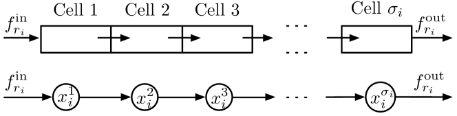
Figure 1: Road discretization and corresponding network model. The portion of road comprised between spatial coordinates $s_{k-1}$ and $s_{k}$, $k\in\{1,\dots,\sigma_{i}\}$ is referred to as cell $k$, and variable $x_{i}^{k}$ denotes the cell density.

We denote by $x_{i}^{k}\in\real$ the traffic density associated with the $k$-th cell of road $r_{i}$, $k\in\{1,\dots,\sigma_{i}\}$. We assume that inflows of vehicles ${f}^{\textup{in}}_{r_{i}}$ enter the road in correspondence of its upstream cell (i.e. $k=1$); accordingly, outflows ${f}^{\textup{out}}_{r_{i}}$ leave the road in correspondence of its downstream cell (i.e. $k=\sigma_{i}$). We model the relation between traffic flows and cell density by assuming that flows of vehicles move in regimes of free flow with constants velocity $\gamma_{i}$, which represents the average speed along link $r_{i}$. Then, the dynamics of the road state $x_{i}=[x_{i}^{1}\,\cdots\,x_{i}^{\sigma_{i}}]^{\mathsf{T}}$ are described by:

$$\begin{bmatrix}\dot{x}_{i}^{1}\\ \dot{x}_{i}^{2}\\ \vdots\\ \dot{x}_{i}^{\sigma_{i}}\end{bmatrix}=\underbrace{\frac{\gamma_{i}}{h}\begin{bmatrix}-1&\\ 1&\scalebox{0.75}[0.9]{$-$}1&\\ &\ddots&\ddots&\\ &&1&0\\ \end{bmatrix}}_{D_{i}}\begin{bmatrix}x_{i}^{1}\\ x_{i}^{2}\\ \vdots\\ x_{i}^{\sigma_{i}}\end{bmatrix}+\begin{bmatrix}{f}^{\textup{in}}_{r_{i}}\\ 0\\ \vdots\\ -{f}^{\textup{out}}_{r_{i}}\end{bmatrix}.$$ (1)

Differently from conventional dynamical models for urban links (e.g. [18]), the space discretization technique (1) allows us to capture the fact that the density of vehicles may not be uniform along the road. Notably, this feature plays a key role in modeling the road outflows in correspondence of signalized intersections (see Section II-B).

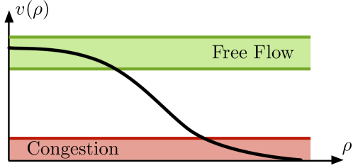
Figure 2: Fundamental diagram describing the static speed-density relation. The almost-flat behavior in regimes of free-flow and heavy congestion allows us to approximate $\gamma(\rho_{i})\approx\gamma_{i}$, as the speed of the of flow is not sensibly affected by changes in density.

Remark 1.

(Equivalence Between (1) and Hydrodynamic Models) The dynamical model (1) derives from the mass-conservation continuity equation [19] in certain traffic regimes, as we explain next. Let the function $\rho_{i}=\rho_{i}(s,t)\geq 0$ denote the (continuous) density of vehicles within road $r_{i}$ at the spatial coordinate $s\in[0,\ell_{i}]$ and time $t\in\mathbb{R}_{\geq 0}$. Let $f_{i}=f_{i}(s,t)\geq 0$ denote the (continuous) flow of vehicles along the road, and let traffic densities and flows follow the hydrodynamic relation

$$\frac{\partial\rho_{i}}{\partial t}+\frac{\partial f_{i}}{\partial s}=0.$$

We first complement the above continuity equation with the Lighthill-Whitham-Richards static relation, $f_{i}=f_{i}(\rho_{i})$, in which traffic flows instantaneously change with the density. Then, we include the speed-density fundamental relation $f_{i}=\rho_{i}v(\rho_{i})$, where $v:\mathbb{R}_{\geq 0}\rightarrow\mathbb{R}_{\geq 0}$ represents the speed of the traffic flow (see Fig. 2), to obtain

$$\frac{\partial\rho_{i}}{\partial t}+\left(v(\rho_{i})+\rho_{i}\frac{d~{}v(\rho_{i})}{d\rho_{i}}\right)\frac{\partial\rho_{i}}{\partial s}=0.$$

Solutions to the above relation are kinematic waves [20] moving at speed $\gamma(\rho_{i})=v(\rho_{i})+\rho_{i}\frac{dv(\rho_{i})}{d\rho_{i}}$. We consider regimes of free flow where the speed of the kinematic wave can be approximated as $\gamma(\rho_{i})\approx\gamma_{i}$. As illustrated in Fig. 2, this approximation is accurate in regimes of free flow or congestion, characterized by $\frac{dv(\rho_{i})}{d\rho_{i}}\approx 0$. Therefore, we let $\gamma_{i}$ denote the average speed of the flow along the link, and consider the approximated continuity equation

$$\frac{\partial\rho_{i}}{\partial t}+\gamma_{i}~{}\frac{\partial\rho_{i}}{\partial s}=0.$$

We then discretize in space the above linear continuity equation, by defining the discrete spatial coordinate

$$s_{k}=kh, k\in\{0,\dots,\sigma_{i}\},$$

and by replacing the partial derivative with respect to $s$ with the difference quotient

$$\frac{\partial\rho_{i}(s_{k},t)}{\partial t}=-\gamma_{i}\;\frac{\rho_{i}(s_{k},t)-\rho_{i}(s_{k-1},t)}{h}.$$

This discretization leads to the dynamical model (1) after introducing the boundaries conditions, represented by inflows ${f}^{\textup{in}}_{r_{i}}$ and outflows ${f}^{\textup{out}}_{r_{i}}$, and by replacing the spatially discretized density $\rho_{i}(s_{k},t)$ with the functions of time $x_{i}^{k}$. $\square$

II-B Model of Intersection and Interconnection Flow

Signalized intersections alternate the right-of-way of vehicles to coordinate and secure conflicting flows between adjacent roads. Every signalized intersection $\mathcal{I}_{j}\in\mathcal{I}$, $j\in\{1,\dots,n_{\mathcal{I}}\}$, is modeled as a set $\mathcal{I}_{j}\subseteq\mathcal{R}\times\mathcal{R}$, consisting of all allowed movements between the intersecting roads. For road $r_{i}\in\mathcal{R}$, let ${\mathcal{I}}_{\textup{in}}^{r_{i}}$ denote the (unique) intersection at the road upstream; similarly, let ${\mathcal{I}}_{\textup{out}}^{r_{i}}$ denote the (unique) intersection at the road downstream. We model the effect of signalized intersections through a set of green split functions $s:\mathcal{R}\times\mathcal{R}\times\mathbb{R}_{\geq 0}\rightarrow\{0,1\}$ that assume boolean values $1$ (green phase) or $0$ (red phase), and let the road inflows be

$$\begin{split}{f}^{\textup{in}}_{r_{i}}&=\sum_{(r_{i},r_{k})\in{\mathcal{I}}_{\textup{in}}^{r_{i}}}s(r_{i},r_{k},t)\,f(r_{i},r_{k})+u_{r_{i}},\\ {f}^{\textup{out}}_{r_{i}}&=\sum_{(r_{k},r_{i})\in{\mathcal{I}}_{\textup{out}}^{r_{i}}}s(r_{k},r_{i},t)\,f(r_{k},r_{i})+w_{r_{i}},\end{split}$$ (2)

where $f:\mathcal{R}\times\mathcal{R}\rightarrow\mathbb{R}_{\geq 0}$ denotes the intersection transmission rate. It is worth noting that the notation $f(r_{i},r_{k})$ represents the transmission rate from road $r_{k}$ to $r_{i}$ and, similarly, $s(r_{i},r_{k},t)$ denotes the green split function that controls traffic flows from $r_{k}$ and directed to $r_{i}$. In (2), we incorporated exogenous inflows and outflows to roads (flows that are not originated or merge to modeled intersections or roads) into ${f}^{\textup{in}}_{r_{i}}$ and ${f}^{\textup{out}}_{r_{i}}$ respectively, by defining the input term $u_{r_{i}}:\mathbb{R}_{\geq 0}\rightarrow\mathbb{R}_{\geq 0}$ and output term $w_{r_{i}}:\mathbb{R}_{\geq 0}\rightarrow\mathbb{R}_{\geq 0}$. We note that $u_{r_{i}}\neq 0$ if and only if $r_{i}\in\mathcal{S}$, and $w_{r_{i}}\neq 0$ if and only if $r_{i}\in\mathcal{D}$.

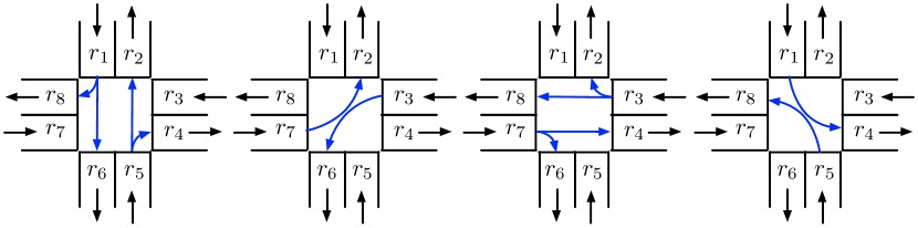
Figure 3: Typical set of phases at a four-ways intersection.

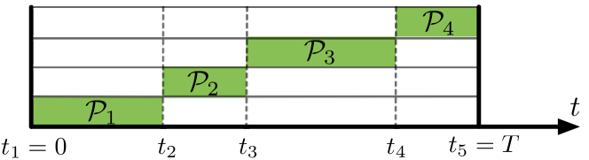
Figure 4: Green splits for the four ways intersection in Fig. 3.

Example 1.

(Example of Intersections and Scheduling Functions) Consider the four-ways intersection illustrated in Fig. 3. The intersection is modeled through the set of allowed movements:

$$\mathcal{I}_{1}=\{(r_{1} ,r_{6}),(r_{1},r_{8}),(r_{5},r_{2}),(r_{5},r_{4}),(r_{7},r_{2}),(r_{3},r_{6}),$$

$$(r_{3},r_{8}),(r_{3},r_{2}),(r_{7},r_{4}),(r_{7},r_{6}),(r_{5},r_{8}),(r_{1},r_{4})\}.$$

Intersections are often partitioned into a group of phases, where each phase represents a set of movements that can occur simultaneously across the intersection. For intersection $\mathcal{I}_{1}$, a typical set of phases is

$$\mathcal{P}_{1} =\{(r_{1},r_{6}),(r_{1},r_{8}),(r_{5},r_{2}),(r_{5},r_{4})\},$$

$$\mathcal{P}_{2} =\{(r_{7},r_{2}),(r_{3},r_{6})\},$$

$$\mathcal{P}_{3} =\{(r_{3},r_{8}),(r_{3},r_{2}),(r_{7},r_{4}),(r_{7},r_{6})\},$$

$$\mathcal{P}_{4} =\{(r_{5},r_{8}),(r_{1},r_{4})\}.$$

The green split function is then defined by alternating the available phases within a cycle time $T\in\mathbb{R}_{\geq 0}$, that is, for all $j\in\{1,\dots,4\}$,

$$s(r_{i},r_{k},t) =\begin{cases}1&\text{if }(r_{i},r_{k})\in\mathcal{P}_{j}\text{ and }t\in[t_{j},t_{j+1}),\\ 0&\text{otherwise},\end{cases}$$

where $t_{j}\in\mathbb{R}_{\geq 0}$ are the switching times. See Fig. 4 for a graphical illustration. $\square$

Next, we make critical use of the underlying road-discretization technique (1), and model transmission rates as functions proportional to the occupancy of the cell at downstream of each road, that is,

$$f(r_{i},r_{k})=c(r_{i},r_{k})x_{k}^{\sigma_{k}},$$ (3)

where $c:\mathcal{R}\times\mathcal{R}\rightarrow\real$ is a parameter that models the speed of the outflow, and includes the average routing ratio of vehicles entering road $r_{i}$ from $r_{k}$. Although (3) constitutes an approximation of the intersection transmission rate, which often contains saturation terms (e.g. see [21] for a discussion), the combination of (3) with the proposed space-discretization technique (1) performs well in practice (see Section V for numerical validation of (3)), at least in the considered regimes.

Remark 2.

(Turning Rates and Conservation of Flows at Intersections) The existence of independent lanes for different turning preferences in proximity of intersections often leads to the decomposition $c(r_{i},r_{k})=\varphi(r_{i},r_{k})\phi(r_{i},r_{k})$, where the function $\varphi:\mathcal{R}\times\mathcal{R}\rightarrow[0,1]$ represents the constant average routing ratio of vehicles entering road $r_{i}$ from $r_{k}$. The conservation of flows at intersections can be guaranteed by letting $\sum_{i}\varphi(r_{i},r_{k})=1$. $\square$

We emphasize that the proposed model represents a simplified framework with respect to traditional, more-established, models. In fact, the assumptions we make are realistic for systems that are operating close to their free-flow regime, and do not take into account collateral phenomena, such as back-propagation in regimes of congestion, which would require ad-hoc adjustments in the model.

II-C Switching and Time-Invariant Traffic Network Dynamics

Individual road dynamics can be combined into a joint network model that captures the interactions among all modeled routes and intersections. To this aim, we adopt an approach similar to [14], and assume that exogenous outflows are proportional to the number of vehicles in the road, that is, $w_{r_{i}}=\bar{w}_{r_{i}}x_{i}^{\sigma_{i}}$, $\bar{w}_{r_{i}}\in[0,1]$. By combining Equations (1), (2) and (3), we obtain

$$\begin{split}\underbrace{\begin{bmatrix}\dot{x}_{1}\\ \dot{x}_{2}\\ \vdots\\ \dot{x}_{{n}_{\textup{r}}}\end{bmatrix}}_{\dot{x}}=\underbrace{\begin{bmatrix}A_{11}&A_{12}&\cdots&A_{1{n}_{\textup{r}}}\\ A_{21}&A_{22}&\ddots&A_{2{n}_{\textup{r}}}\\ \vdots&\ddots&\ddots&\vdots\\ A_{{n}_{\textup{r}}1}&A_{{n}_{\textup{r}}2}&\cdots&A_{{n}_{\textup{r}}{n}_{\textup{r}}}\\ \end{bmatrix}}_{A}\underbrace{\begin{bmatrix}x_{1}\\ x_{2}\\ \vdots\\ x_{{n}_{\textup{r}}}\end{bmatrix}}_{x}+\quad\quad\quad\quad\quad&\\ +\underbrace{\begin{bmatrix}I_{n_{1}}&0&\cdots&0\\ 0&I_{n_{2}}&\ddots&0\\ \vdots&\ddots&\ddots&\vdots\\ 0&0&\cdots&I_{{n}_{\textup{r}}}\\ \end{bmatrix}}_{B}\underbrace{\begin{bmatrix}u_{1}\\ u_{2}\\ \vdots\\ u_{{n}_{\textup{r}}}\end{bmatrix}}_{u},&\end{split}$$ (4)

where $A\in{}^{n\times n}$, $n=\sum_{i=1}^{{n}_{\textup{r}}}\sigma_{i}$ is the overall number of modeled network cells, $u$ derives from (2), and

$$A_{ik}\!\! =\!\!\begin{cases}s(r_{i},r_{k},t)c(r_{i},r_{k})e_{1}e_{\sigma_{k}}^{\mathsf{T}},&\text{if }i\neq k,\\ D_{i}\!-\!\left(\sum_{\ell}s(r_{\ell},r_{i},t)c(r_{\ell},r_{i})+\bar{w}_{r_{i}}\right)e_{\sigma_{i}}e_{\sigma_{i}}^{\mathsf{T}},&\text{if }i=k,\end{cases}$$

where $e_{i}\in{}^{\sigma_{i}}$ denotes the $i$-th canonical vector of size $\sigma_{i}$.

We note that the matrix $A$ in (4) is typically sparse, because not all roads are adjacent in the network interconnection, and its sparsity pattern varies over time as determined by the green splits $s(r_{i},r_{k},t)$. Thus, the network model (4) represents a linear switching system, where the switching signals are the green split functions.

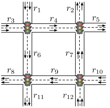
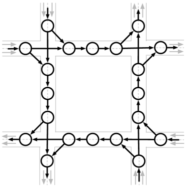
Figure 5: Network model associated with a traffic network composed of $n_{\mathcal{I}}=4$ intersections and ${n}_{\textup{r}}=12$ roads. Each road is associated with a set of states that represent the density of the cells within the roads.

Example 2.

(Example of Traffic Network) Consider the network illustrated in Fig. 5, with $\mathcal{R}=\{r_{1},\dots,r_{12}\}$ and $\mathcal{I}=\{\mathcal{I}_{1},\dots,\mathcal{I}_{4}\}$. The network comprises four destination roads $\mathcal{D}=\{r_{2},r_{5},r_{8},r_{11}\}$ ($\bar{w}_{r_{i}}=1$ for all $r_{i}\in\mathcal{D}$, and $\bar{w}_{r_{i}}=0$ otherwise), and four source roads ($\mathcal{S}=\{r_{1},r_{3},r_{10},r_{12}\}$, with $u_{r_{i}}\neq 0$ only if $r_{i}\in\mathcal{S}$). Let $\ell_{i}/h=3$ and $\gamma_{i}/h=3$ for all $i\in\{1,\dots,n_{r}\}$. Then, the matrices in (4) read as

$$A_{ii} =\begin{bmatrix}-1\\ 1&-1\\ &1&-\left(\sum_{\ell}s(r_{\ell},r_{i},t)c(r_{\ell},r_{i})+\bar{w}_{r_{i}}\right)\end{bmatrix},$$

$$A_{ij} =\begin{bmatrix}0&\quad\;0&\quad\quad\quad\;s(r_{i},r_{j},t)c(r_{i},r_{j})\quad\quad\quad\quad\\ 0&\quad\;0&0\\ 0&\quad\;0&0\end{bmatrix},$$

for all $i,j\in\{1,\dots,{n}_{\textup{r}}\}$. Notice that $s(r_{i},r_{j},t)=0$ for all times if $(r_{j},r_{k})\not\in\mathcal{I}_{k}$ for all $k\in\{1,\dots,n_{\mathcal{I}}\}$.

$\square$

Next, we make the typical assumption that scheduling functions are periodic, with period $T\in{}_{>0}$. That is, for all $(r_{i},r_{k})\in\mathcal{I}_{j}$, $j\in\{1,\dots,n_{\mathcal{I}}\}$, and for all times $t$:

$$s(r_{i},r_{k},t)=s(r_{i},r_{k},t+T).$$

Let $\mathcal{T}=\{\tau_{1},\dots,\tau_{m}\}$ denote the set of time instants when a scheduling function changes its value, that is,

$$\mathcal{T}=\{\tau\in[0,T]\;:\;\exists( r_{i},r_{k})\in\mathcal{I},$$

$$\lim_{t\rightarrow\tau^{-}}\!\!s(r_{i},r_{k},t)\!\neq\!\!\lim_{t\rightarrow\tau^{+}}\!\!s(r_{i},r_{k},t)\}.$$

Notice that the network matrix A in (4) remains constant between any consecutive time instants $\tau_{i-1}$ and $\tau_{i}$. We denote each constant matrix by $A_{i}$, and refer to it as to the $i$-th network mode. Further, let $d_{i}=\tau_{i}-\tau_{i-1}$, with $i\in\{1,\dots,m\}$ and $\tau_{0}=0$, denote the duration of the $i$-th network mode. We employ a state-space averaging technique [22] and define a linear-time invariant approximation of the switching network model (4):

$${\dot{x}}_{\textup{av}}={A}_{\textup{av}}{x}_{\textup{av}}+B{u}_{\textup{av}},$$ (5)

where ${A}_{\textup{av}}=\frac{1}{T}\sum_{i=1}^{m}d_{i}A_{i}$, and ${u}_{\textup{av}}=[{u}_{\textup{av,$1$}}\dots u_{\textup{av,${n}_{\textup{r}}$}}]$, ${u}_{\textup{av,$i$}}=(1/T)\int_{0}^{T}u_{i}(\tau)~{}d\tau$. We note that the averaging technique preserves the sparsity pattern of the network, that is, ${A}_{\textup{av}}(i,j)\neq 0$ if and only if $A_{k}(i,j)\neq 0$ for some $k$.

In general, the approximation of the behavior of the switching system (4) with the average dynamics (5) is accurate if the operating period $T$ is short in comparison to the underlying system dynamics. Under suitable technical assumptions, the deviation of average models with respect to the network instantaneous state has been characterized in e.g. [15]. In [15], the authors formally provide a bound on the accuracy of the approximation, where the bound becomes tighter for decreasing values of $T$, and increasing values of road lengths. Although a formal characterization of the performance of average model is often an extremely challenging task, and the formal results in [15] hold for a single roads in the presence of a single signalized intersections, the accuracy of averaging techniques has been shown to be satisfactory in similar applications (see e.g. [16]). A numerical validation of the averaging technique, and its validity in relation to the cycle-time $T$, is discussed in Section V (see Fig. 7).

II-D Problem Formulation

In this paper, we consider the dynamical model (5) and focus on the problem of designing the durations of the green split functions so that a measure of network congestion is optimized. As illustrated through the relation ${A}_{\textup{av}}=\frac{1}{T}\sum_{i=1}^{m}d_{i}A_{i}$ (see (5)), the average model allows us to design the durations of the network modes, rather than their exact sequence. This approach motivates the adoption of a two-stage optimization process. First, the durations of the modes is optimized by considering a joint model that captures the dynamics of the entire interconnection. Second, offset control techniques (see e.g. [7]) can be employed to decide the specific sequence of phases, given the durations of the splits and by considering local interconnection models. In this paper, we focus on the first stage. To formalize our optimization problem, we denote by ${y}_{\textup{av}}$ the vector of the queue lengths originated by the signalized intersections, and model ${y}_{\textup{av}}$ as the occupancy of the cells at roads downstream, that is,

$${y}_{\textup{av}}={C}_{\textup{av}}{x}_{\textup{av}},\; \;{C}_{\textup{av}}=\begin{bmatrix}e_{\sigma_{1}}^{\mathsf{T}}&\dots&0\\ \vdots&\ddots\\ 0&\dots&e_{\sigma_{{n}_{\textup{r}}}}^{\mathsf{T}}\end{bmatrix}.$$ (6)

We assume the network is initially at a certain initial state $x_{0}$, and focus on the problem of optimally designing the mode durations $\{d_{1},\dots d_{m}\}$ that minimize the $\mathcal{H}_{2}$-norm of the vector of queue lengths ${y}_{\textup{av}}$. Namely, we consider the following dynamical optimization problem:

$$\min_{d_{1},\dots,d_{m}}\;\;\;\;\;\; \int_{0}^{\infty}\|{y}_{\textup{av}}\|_{2}^{2}~{}dt,$$

subject to $${\dot{x}}_{\textup{av}}={A}_{\textup{av}}{x}_{\textup{av}},$$ (7a)

$${y}_{\textup{av}}={C}_{\textup{av}}{x}_{\textup{av}},$$ (7b)

$${x}_{\textup{av}}(0)=x_{0},$$ (7c)

$${A}_{\textup{av}}=\frac{1}{T}\left(d_{1}A_{1}+\dots+d_{m}A_{m}\right),$$ (7d)

$$T=d_{1}+\dots+d_{m},$$ (7e)

$$d_{i}\geq 0\quad i\in\{1,\dots,m\}.$$ (7f)

Loosely speaking, the optimization problem (7) seeks for an optimal set of split durations that minimize the $\mathcal{L}_{2}$-norm of the impulse-response of the system to the initial conditions $x_{0}$. Thus, similarly to [23], our framework considers the “cool down” period. In this scenario, exogenous inflows and outflows are not known a priori, and the goal is to evacuate the network as fast as possible, where the final condition is an empty system. Under this assumption, ${A}_{\textup{av}}$ and the solution to (7), shall be re-computed when the current traffic conditions $x_{0}$ change significantly. Finally, we note that constraint (7e) guarantees feasibility of the resulting solutions. In fact, the time-normalization in (7e) implies that for any solution resulting from (7), there exists (at least) one sequence of movements at each intersection, with overall cycle time $T$, and that abide the selected set of durations.

III Design of Optimal Network Mode Durations

In this section, we propose a numerical method to determine solutions to the optimization problem (7). The approach we discuss is centralized, namely, it requires knowledge of the state $x_{0}$ for all network cells. An extension of the framework to fit a distributed implementations is then discussed in Section IV. At its core, the technique relies on rewriting the cost function of (7) in relation to the controllability Gramian of an appropriately-defined linear system, as we explain next.

Lemma 2.

(Controllability Gramian Cost Function) Let

$$\mathcal{W}({A}_{\textup{av}},x_{0})=\int_{0}^{\infty}e^{{A}_{\textup{av}}t}x_{0}x_{0}^{\mathsf{T}}e^{{A}_{\textup{av}}^{\mathsf{T}}t}~{}~{}dt.$$

The following minimization problem is equivalent to (7):

$$\underset{d_{1},\dots,d_{m}}{\text{ min }}\;\;\; \quad\operatorname{Trace}\left({C}_{\textup{av}}~{}\mathcal{W}({A}_{\textup{av}},x_{0})~{}{C}_{\textup{av}}^{\mathsf{T}}\right),$$

subject to $$\quad{A}_{\textup{av}}=\frac{1}{T}\left(d_{1}A_{1}+\dots+d_{m}A_{m}\right),$$

$$\quad T=d_{1}+\dots+d_{m},$$

$$\quad d_{i}\geq 0,\quad i\in\{1,\dots,m\}.$$ (8)

Proof.

By incorporating (7a), (7b), and (7c) into the cost function of optimization problem (7), we can rewrite:

$$\int_{0}^{\infty}\|{y}_{\textup{av}}\|_{2}^{2}~{}dt =\int_{0}^{\infty}x_{0}^{\mathsf{T}}e^{{A}_{\textup{av}}^{\mathsf{T}}t}{C}_{\textup{av}}^{\mathsf{T}}{C}_{\textup{av}}e^{{A}_{\textup{av}}t}x_{0}~{}dt$$

$$=\operatorname{Trace}\left(\int_{0}^{\infty}x_{0}^{\mathsf{T}}e^{{A}_{\textup{av}}^{\mathsf{T}}t}{C}_{\textup{av}}^{\mathsf{T}}{C}_{\textup{av}}e^{{A}_{\textup{av}}t}x_{0}~{}dt\right)$$

$$=\int_{0}^{\infty}\operatorname{Trace}\left({C}_{\textup{av}}e^{{A}_{\textup{av}}t}x_{0}x_{0}^{\mathsf{T}}e^{{A}_{\textup{av}}^{\mathsf{T}}t}{C}_{\textup{av}}^{\mathsf{T}}\right)dt$$

$$=\operatorname{Trace}\left({C}_{\textup{av}}\int_{0}^{\infty}e^{{A}_{\textup{av}}t}x_{0}x_{0}^{\mathsf{T}}e^{{A}_{\textup{av}}^{\mathsf{T}}t}dt~{}{C}_{\textup{av}}^{\mathsf{T}}\right),$$

from which the claimed statement follows. ∎

Next, we note that the cost function of (7) is finite only if the choice of parameters $\{d_{1},\dots,d_{m}\}$ leads to a dynamical matrix ${A}_{\textup{av}}$ that is Hurwitz-stable. Requiring Hurwitz-stability of ${A}_{\textup{av}}$ corresponds to imposing $\alpha({A}_{\textup{av}})<0$, where $\alpha({A}_{\textup{av}}):=\sup\{\Re(s):s\in\mathbb{C},\det(sI-{A}_{\textup{av}})=0\}$ denotes the spectral abscissa of ${A}_{\textup{av}}$. The following result proves network stability under optimal sets of split durations.

Theorem 3.

(Stability of Optimal Solutions) Consider a traffic network $\mathcal{N}=(\mathcal{R},\mathcal{I})$, and assume that there exists a path from every node in $\mathcal{N}$ to at least one node in $\mathcal{D}$. Let $s(r_{i},r_{k},\bar{t})\neq 0$ for all $(r_{i},r_{k})\in\mathcal{I}$, and for some $\bar{t}\in[0,T]$. Then,

$$\alpha({A}_{\textup{av}})<0.$$

Proof.

From the structure of (4) and from the assumption $s(r_{i},r_{k},\bar{t})\neq 0$ follows that ${A}_{\textup{av}}(i,i)<0$ for all $i\in\{1,\dots,n\}$, while ${A}_{\textup{av}}(i,j)\geq 0$ for all $j\in\{1,\dots,n\}$, $j\neq i$. Moreover, all columns of ${A}_{\textup{av}}$ have nonpositive sum. In particular, the columns corresponding to destination cells have strictly negative sum, that is, $\sum_{i=1}^{n}{A}_{\textup{av}}(i,j)\leq 0$ for all $j\in\{1,\dots,n\}$, and $\sum_{i=1}^{n}{A}_{\textup{av}}(i,j)<0$ for all $j$ such that $r_{j}\in\mathcal{D}$. To show $\alpha({A}_{\textup{av}})<0$, we use the fact that destination cells in $\mathcal{D}$ have no departing edges, and re-order the states so that

$${A}_{\textup{av}}=\begin{bmatrix}A_{11}&0\\ A_{21}&A_{22}\end{bmatrix},$$

where $A_{22}\in{}^{n_{d}\times n_{d}}$, $n_{d}=|\mathcal{D}|$, is the submatrix that describes the dynamics of the destination cells, $A_{11}\in{}^{(n-n_{d})\times(n-nd)}$, and $A_{21}\in{}^{n_{d}\times(n-nd)}$. The fact $\alpha(A_{22})<0$ immediately follows from (2). The stability of $A_{11}$ follows from the connectivity assumption in the original network, and from the analysis of grounded Laplacian matrices (see e.g. [24, Theorem 1]). ∎

For the solution of the optimization problem (2), we propose a method based on a generalization of the concept of spectral abscissa, namely, the smoothed spectral abscissa. For a dynamical system of the form (5)-(6), the smoothed spectral abscissa [17] is defined as the root $\tilde{\alpha}\in\real$ of the implicit equation

$$\operatorname{Trace}\left({C}_{\textup{av}}~{}\mathcal{W}({A}_{\textup{av}}-\tilde{\alpha}I,B)~{}{C}_{\textup{av}}^{\mathsf{T}}\right)=\epsilon^{-1},$$ (9)

where $\epsilon\in{}_{\geq 0}$. It is worth noting that the root $\tilde{\alpha}$ is unique [17], and for fixed $B$ and ${C}_{\textup{av}}$ it is a function of both $\epsilon$ and ${A}_{\textup{av}}$, namely $\tilde{\alpha}(\epsilon,{A}_{\textup{av}})$.

Remark 3.

(Properties of the Smoothed Spectral Abscissa) For any $\epsilon>0$, the smoothed spectral abscissa is an upper bound to $\alpha(A)$, and this bound becomes exact as $\epsilon\rightarrow 0$. To see this, we first observe that the integral $\int_{0}^{\infty}e^{({A}_{\textup{av}}-\tilde{\alpha}I)t}BB^{\mathsf{T}}e^{({A}_{\textup{av}}-\tilde{\alpha}I)^{\mathsf{T}}t}dt$ exists and is finite for any $\tilde{\alpha}>\alpha({A}_{\textup{av}})$, as the function $e^{({A}_{\textup{av}}-\tilde{\alpha}I)t}$ is bounded and convergent as $t\rightarrow+\infty$. On the other hand, for any $\tilde{\alpha}<\alpha({A}_{\textup{av}})$ the function $e^{({A}_{\textup{av}}-\tilde{\alpha}I)t}$ becomes unbounded for $t\rightarrow+\infty$ and the above integral is infinite. It follows that, the left-hand side of (9) is finite only if $\tilde{\alpha}>\alpha(A)$ or, in other words, for any finite $\epsilon$, $\tilde{\alpha}$ satisfies $\tilde{\alpha}>\alpha(A)$. $\square$

We observe that, by letting $\tilde{\alpha}=0$ in (9), the optimization problem (2) can equivalently be reformulated in terms of the smoothed spectral abscissa as follows:

$$\underset{d_{1},\dots,d_{m},\epsilon}{\text{ min }}\;\;\; \quad\epsilon^{-1},$$

subject to $$\quad{A}_{\textup{av}}=\frac{1}{T}\left(d_{1}A_{1}+\dots+d_{m}A_{m}\right),$$

$$\quad T=d_{1}+\dots+d_{m},$$

$$\quad d_{i}\geq 0,\quad i\in\{1,\dots,m\},$$

$$\quad\tilde{\alpha}(\epsilon,{A}_{\textup{av}})=0,$$ (10)

where the parameter $\epsilon$ is now an optimization variable. In what follows, we denote with $\{d_{1}^{*},\dots,d_{m}^{*},\epsilon^{*}\}$ the value of the optimization parameters at optimality of (III). Problem (III) is a nonlinear optimization problem [17], because the optimization variables $\{d_{1},\dots,d_{m}\}$ and $\epsilon$ are related by means of the nonlinear equation (9).

For the solution of (III), we propose an iterative two-stages numerical optimization process. In the first stage, we fix the value of $\epsilon$ and seek for a choice of $\{d_{1},\dots d_{m}\}$ that leads to a smoothed spectral abscissa that is identically zero. In other words, we let $\epsilon=\bar{\epsilon}$, and solve the following minimization problem:

$$\underset{d_{1},\dots,d_{m}}{\text{min }}\;\;\; \quad|\tilde{\alpha}(\bar{\epsilon},{A}_{\textup{av}})|$$

subject to $$\quad{A}_{\textup{av}}=\frac{1}{T}\left(d_{1}A_{1}+\dots+d_{m}A_{m}\right),$$

$$\quad T=d_{1}+\dots+d_{m},$$

$$\quad d_{i}\geq 0,\quad i\in\{1,\dots,m\}.$$ (11)

It is worth noting that every ${\bar{A}}_{\textup{av}}$ that is solution to (III) and that satisfies $\tilde{\alpha}(\bar{\epsilon},{\bar{A}}_{\textup{av}})=0$, is a point in the feasible set of (III), which corresponds to a cost of congestion $\int_{0}^{\infty}\|{y}_{\textup{av}}\|_{2}^{2}~{}dt=1/{\bar{\epsilon}}$.

In the second stage, we perform a line-search over the parameter $\epsilon$, where the value of $\epsilon$ is increased at every iteration until the minimizer $\epsilon^{*}$ is achieved. We note that the optimizer of (III) with $\epsilon=\epsilon^{*}$ is indeed $\{d_{1}^{*},\dots,d_{m}^{*}\}$, an optimal solution to (III). Thus, heuristically, the progressive $\epsilon$-update step in the two stages optimization problem allows us to determine (local) solutions to (III).

The remainder of this section is devoted to the description of the two-stage optimization process. The benefit of solving (III) as opposed to (III) is that we can derive an expression for the gradient of $\tilde{\alpha}_{\bar{\epsilon}}$ with respect to the mode durations $\{d_{1},\dots,d_{m}\}$, as we illustrate next. In the remainder of this section, with a slight abuse of notation, we use the compact form $\tilde{\alpha}(\bar{\epsilon},{A}_{\textup{av}})=\tilde{\alpha}_{\bar{\epsilon}}$ and, for a matrix $M=[m_{ij}]\in{}^{m\times n}$, we denote its vectorization by ${M}^{\textup{v}}=[m_{11}\dots m_{m1},m_{12}\dots m_{mn}]^{\mathsf{T}}$.

Lemma 4.

(Descent Direction) Let $\tilde{\alpha}_{\bar{\epsilon}}$ denote the unique root of (9) with $\bar{\epsilon}\in{}_{>0}$. Let $d=[d_{1},\dots,d_{m}]^{\mathsf{T}}$, and let $K=[{A}^{\textup{v}}_{1}~{}{A}^{\textup{v}}_{2}~{}\dots~{}{A}^{\textup{v}}_{m}]$. Then,

$$\frac{\partial\tilde{\alpha}_{\bar{\epsilon}}}{\partial d}=K^{\mathsf{T}}{\left(\frac{QP}{\operatorname{Trace}\left(QP\right)}\right)}^{\textup{v}}$$

where $P\in{}^{n\times n}$ and $Q\in{}^{n\times n}$ are the unique solution to the two Lyapunov equations

$$({A}_{\textup{av}}-\tilde{\alpha}_{\bar{\epsilon}}I)~{}P +P({A}_{\textup{av}}-\tilde{\alpha}_{\bar{\epsilon}}I)^{\mathsf{T}}+x_{0}x_{0}^{\mathsf{T}}\;=0,$$

$$({A}_{\textup{av}}-\tilde{\alpha}_{\bar{\epsilon}}I)^{\mathsf{T}}Q +Q({A}_{\textup{av}}-\tilde{\alpha}_{\bar{\epsilon}}I)~{}+{C}_{\textup{av}}{C}_{\textup{av}}^{\mathsf{T}}=0,$$ (12)

and $I\in{}^{n\times n}$ denotes the identity matrix.

Proof.

The expression for the partial derivative of the smoothed spectral abscissa with respect to $d$ can be obtained from the composite function

$$\frac{\partial\tilde{\alpha}_{\bar{\epsilon}}}{\partial d}=\frac{\partial{A}_{\textup{av}}}{\partial d}~{}\frac{\partial\tilde{\alpha}_{\bar{\epsilon}}}{\partial{A}_{\textup{av}}},$$

where $\frac{\partial{A}_{\textup{av}}}{\partial d}$ follows immediately from (7d), and the expression for the derivative of $\tilde{\alpha}_{\bar{\epsilon}}$ with respect to ${A}_{\textup{av}}$ is given in [17, Theorem 3.2]. ∎

We note that equations (4) always admit unique solution. To see this, we use the fact that $\tilde{\alpha}$ is an upper bound to $\alpha({A}_{\textup{av}})$, and observe that $({A}_{\textup{av}}-\tilde{\alpha}_{\bar{\epsilon}}I)$ is Hurwitz-stable for every ${A}_{\textup{av}}$.

A gradient descent method based on Lemma 4 is illustrated in Algorithm 1. Each iteration of the algorithm comprises the following steps. First, (lines $4-7$) a (possibly non feasible) descent direction $\nabla$ is derived as illustrated in Lemma 4. Second, (line $8-9$) a gradient-projection technique [25] is used to enforce constraints (7d)-(7f). The update-step follows (line $10$).

Input: Matrix ${C}_{\textup{av}}$, vector $x_{0}$, scalars $\xi$, $\mu$

Output: $\{d_{1}^{*},\dots d_{m}^{*},\epsilon^{*}\}$ solution to (7)

1 Initialize: $d^{(0)}$, $\bar{\epsilon}=0$, $k=1$

2 while $\tilde{\alpha}_{\bar{\epsilon}}^{(k)}=0$ do

3       repeat

4             Compute $\tilde{\alpha}_{\bar{\epsilon}}^{(k)}$ by solving (9);

5             Solve for $P$ and $Q$: $({A}_{\textup{av}}^{(k)}-\alpha_{\bar{\epsilon}}^{(k)}I)P+P({A}_{\textup{av}}^{(k)}-\alpha_{\bar{\epsilon}}^{(k)}I)^{\mathsf{T}}+x_{0}x_{0}^{\mathsf{T}}=0$; $({A}_{\textup{av}}^{(k)}-\alpha_{\bar{\epsilon}}^{(k)}I)^{\mathsf{T}}Q+Q({A}_{\textup{av}}^{(k)}-\alpha_{\bar{\epsilon}}^{(k)}I)+{C}_{\textup{av}}{C}_{\textup{av}}^{\mathsf{T}}=0$;

6             $\frac{\partial\alpha_{\bar{\epsilon}}^{(k)}}{\partial d}\leftarrow\frac{QP}{\operatorname{Trace}(QP)}$;

7             $\nabla\leftarrow\tilde{\alpha}_{\bar{\epsilon}}\frac{\partial\alpha_{\bar{\epsilon}}^{(k)}}{\partial d}$;

8             Compute projection matrix $\mathcal{P}^{(k)}$;

9             $d^{(k)}\leftarrow d^{(k)}-\mu~{}\mathcal{P}^{(k)}\nabla$;

10             ${A}_{\textup{av}}^{(k)}\leftarrow\frac{1}{T}\left(d_{1}A_{1}+\dots+d_{m}A_{m}\right)$;

11             $k\leftarrow k+1$;

12            

13      until $\mathcal{P}^{(k)}\nabla=0$;

14      $\bar{\epsilon}\leftarrow\bar{\epsilon}+\xi$;

15      

16 end while

17return $d$;

Algorithm 1 Centralized solution to (7).

Algorithm 1 employs a fixed stepsize $\mu\in(0,1)$, and a terminating criterion (line $13$) based on the Karush-Kuhn-Tucker conditions for projection methods [25]. The $\epsilon$-update step, which constitutes the outer while-loop (line $2-14$), is then performed at each iteration of the gradient descent phase, and the line-search is terminated when $|\tilde{\alpha}_{\epsilon}|=0$ cannot be achieved. To prevent the algorithm from stopping at local minimas, the gradient descent algorithm can be repeated over multiple feasible initial conditions $d^{(0)}$.

Remark 4.

(Complexity of Algorithm 1) The computational complexity of Algorithm 1 in relation to the network size can be derived as follows. First, the computation of the current value of the smoothed spectral abscissa can be achieved via a root-finding algorithm (such as the bisection algorithm) over the implicit function (9). The complexity of this operation is a logarithmic function of the desired accuracy, and it requires the computation of the trace of the Gramian matrix. Thus, for given accuracy, the complexity of this operation is $\mathcal{O}(n)$. Second, Algorithm 1 requires to determine solutions to the pair of Lyapunov equations (4). Modern methods to solve Lyapunov equations [26] rely on the Schur decomposition of the matrix ${A}_{\textup{av}}$, whose complexity is $\mathcal{O}(n^{3})$. It is worth noting that, given the Schur decomposition ${A}_{\textup{av}}=UTU^{\mathsf{T}}$, where $T$ is upper triangular and $U$ is unitary, a decomposition for $({A}_{\textup{av}}-\tilde{\alpha}I)$ follows immediately by shifting $T$ to $(T-\tilde{\alpha}I)$. Therefore, a single decomposition is required at each iteration of the gradient descent and the complexity of Algorithm 1 is therefore $\mathcal{O}(n^{3})$. $\square$

IV Distributed Gradient Descent

The centralized computation of $\{d_{1}^{*},\dots,d_{m}^{*},\epsilon^{*}\}$ assumes complete knowledge of the matrices $A_{1},\dots A_{m}$, and requires to numerically solve the pair of Lyapunov equations (4). For large-scale traffic networks, such computation imposes a limitation in the dimension of the matrix ${A}_{\textup{av}}$ and, consequently, on the number of signalized intersections that can be optimized simultaneously. Since the performance of the proposed optimization technique depends upon the possibility of modeling and optimizing large network interconnections, a limitation on the number of modeled roads and intersections constitutes a bottleneck toward the development of more efficient traffic infrastructures. A possible solution to address this complexity issue is to distribute the computation of the descent direction in Algorithm 1 among a group of agents, in a way that each agent is responsible for a subpart of the entire computation (e.g. see Fig. 6). Agents can represent geographically-distributed control centers or clusters in parallel computing, each responsible for the control of a group of intersections.

In order to distribute the computation of solutions to (4), in this section we focus on distributively solving Lyapunov equations of the form

$$\Lambda X+X\Lambda^{\mathsf{T}}+D=0,$$ (13)

where $X=X^{\mathsf{T}}\in{}^{n\times n}$ is an unknown matrix, $D=D^{\mathsf{T}}\in{}^{n\times n}$, $\Lambda\in{}^{n\times n}$. Let $\Lambda$ be partitioned as

$$\Lambda=\Lambda_{1}+\dots+\Lambda_{\nu},$$

where $\Lambda_{i}\in{}^{n\times n}$, $i\in\{1,\dots,\nu\}$. We assume that each agent $i$ knows $\Lambda_{i}$ only. Note that $\Lambda_{i}$ are sparse matrices, and their sparsity pattern depends upon the subpart of infrastructure associated with that agent. In addition, we assume that neighboring agents are allowed to exchange information by means of a communication infrastructure. Let $\mathcal{G}=(\mathcal{V},\mathcal{E})$ be the communication graph, where each vertex $i\in\{1,\dots,\nu\}$ represents one agent, and $\mathcal{E}\subseteq\mathcal{V}\times\mathcal{V}$ represents the interconnection. The following lemma constitutes the key ingredient of the method we propose to distributively compute $X$.

Lemma 5.

(Distributed Solutions to (13)) Consider a Lyapunov equation of the form (13), and let $\Lambda$ be Hurwitz-stable. The following statements are equivalent:

1. $X^{*}$ solves (13);

2. For all $i\in\{1,\dots,\nu\}$, there exists $D_{i}\in{}^{n\times n}$ s.t.

   $$\Lambda_{i}X^{*}+X^{*}\Lambda_{i}^{\mathsf{T}}+D_{i}=0,\text{ and }\sum_{i=1}^{\nu}D_{i}=D.$$

Proof.

In order to prove the claim, we first observe that under the assumption of Hurwitz-stability for $\Lambda$, the solution $X^{*}$ to (13) is unique.
$(i)\Rightarrow(ii).$ Let $X^{*}$ denote the unique solution to (13). By expanding $\Lambda=\Lambda_{1}+\dots+\Lambda_{\nu}$, we obtain

$$\sum_{i=1}^{\nu}(\Lambda_{i}X^{*}+X^{*}A_{i}^{\mathsf{T}})+D=0.$$

Thus, by letting $D_{i}=-(\Lambda_{i}X^{*}+X^{*}A_{i}^{\mathsf{T}})$, $(ii)$ immediately follows.
$(ii)\Rightarrow(i).$ Let $(\tilde{X}$, $\tilde{D}_{1},\dots,\tilde{D}_{\nu})$ satisfy $(ii)$, that is, for all $i\in\{1,\dots,\nu\}$

$$\Lambda_{i}\tilde{X}+\tilde{X}\Lambda_{i}^{\mathsf{T}}+\tilde{D}_{i}=0, \sum_{i=1}^{\nu}\tilde{D}_{i}=\tilde{D}.$$

Notice that the existence of the solution to (13) guarantees the existence of $(\tilde{X}$, $\tilde{D}_{1},\dots,\tilde{D}_{\nu})$. By substitution, we obtain $-\sum_{i+1}^{\nu}(\Lambda_{i}\tilde{X}+\tilde{X}\Lambda_{i}^{\mathsf{T}})=D$, or in other words, $\tilde{X}$ satisfies $\Lambda\tilde{X}+\tilde{X}\Lambda^{\mathsf{T}}+D=0$. The uniqueness of the solution to (13) implies $\tilde{X}=X^{*}$ and concludes the proof. ∎

The method we propose is based on a simultaneous and cooperative reconstruction of the matrices $X^{*}$ and $D_{i}$, and is described next. For all $i\in\{1,\dots,\nu\}$, we let $\bar{\Lambda}_{i}=\Lambda_{i}\otimes I+I\otimes\Lambda_{i}$. Then, Lemma 5 allows us to restate (13) as a system of equations of the form

$$\underbrace{\begin{bmatrix}\bar{\Lambda}_{1}&I&0&\cdots&0\\ \bar{\Lambda}_{2}&0&I&&\vdots\\ \vdots&\vdots&\ddots&\ddots\\ 0&I&\cdots&I&I\end{bmatrix}}_{H}\underbrace{\begin{bmatrix}{X}^{\textup{v}}\\ {D}^{\textup{v}}_{1}\\ \vdots\\ {D}^{\textup{v}}_{\nu}\end{bmatrix}}_{w}=\underbrace{\begin{bmatrix}0\\ 0\\ \vdots\\ {D}^{\textup{v}}\end{bmatrix}}_{z},$$ (14)

where ${X}^{\textup{v}},{D}^{\textup{v}}_{1},\dots,{D}^{\textup{v}}_{\nu}$ are now the unknown parameters.

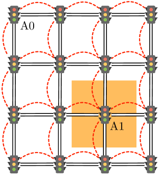
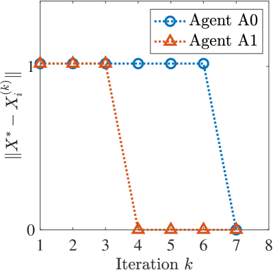
Figure 6: Manhattan-like traffic network and convergence of the distributed algorithm (i)-(iv). (a) Each agent, represented by a signalized intersection, has local knowledge of the road interconnection (continuous black lines) and is allowed to communicate with neighboring intersections (dashed red lines). Shaded area depicts the subset information that is available to agent A1. (b) Error between distributed solution and centralized solution vs iterations. The plot illustrates how internal agents (e.g. A1) show faster convergence due to shorter longest paths within the graph.

In order to distribute the computation of the vector $w$ (and thus $X^{*}$) among the $\nu$ distributed agents, we let

$$H_{i}=\begin{bmatrix}\bar{\Lambda}_{i}&0&\cdots&I&\cdots&0\\ 0&I&\cdots&&\cdots&I\end{bmatrix},\quad\quad z_{i}=\begin{bmatrix}0\\ {D}^{\textup{v}}\end{bmatrix},$$

for all $i\in\{1,\dots,\nu\}$. At every iteration $k$, each agent $i$ constructs a local estimate $\hat{w}^{(k+1)}_{i}$ (correspondingly $\hat{X}^{(k)}_{i}$) by performing the following operations in order:

1. Receive $\hat{w}^{(k)}_{j}$ and $K_{j}^{(k)}$ from neighbor $j$;

2. $\hat{w}^{(k+1)}_{i}=\hat{w}^{(k)}_{i}+[K_{i}^{(k)}~{}0][K_{i}^{(k)}~{}K_{j}^{(k)}]^{\dagger}(\hat{w}^{(k)}_{i}-\hat{w}^{(k)}_{j})$;

3. $K_{i}^{(k+1)}=\operatorname{Basis}(\text{Im}(K_{i}^{(k)})\cap\text{Im}(K_{i}^{(k)}))$;

4. Transmit $\hat{w}^{(k+1)}_{i}$ and $K_{i}^{(k+1)}$ to neighbor $j$;

where,

$$\hat{w}_{i}^{(0)}=H_{i}^{\dagger}z_{i},\quad\quad K_{i}^{(0)}=\operatorname{Basis}(\operatorname{Ker}(H_{i})).$$

While the convergence of the procedure (i)-(iv) can be ensured by means of an approach similar to [27], in this paper we focus on providing numerical validation to the algorithm, in the framework of transportation systems. To this aim, we consider the Manhattan-like network interconnection depicted in Fig. 6 [28], and assume that each traffic intersection is equipped with a computational unit that is responsible for a subpart of the computation of (4). In other words, every traffic intersection denotes one agent of the communication graph $\mathcal{G}$, and is allowed to exchange information with neighboring intersections by means of communication channels (dashed-red lines in Fig. 6). We make the practical assumption that each agent has the sole knowledge of: (i) the local structure of the traffic interconnection, that is, the geographical layout of roads adjacent to that intersections (shaded area in Fig. 6), and (ii) the current travel time of roads adjacent to that intersection.

We numerically illustrate in Fig.6 the convergence of the distributed procedure (i)-(iv), where we compare the accuracy of the local estimate $\hat{X}^{(k)}_{i}$ with respect to the centralized solution $X^{*}$, as a function of the iteration $k$. As discussed in [27], this class of procedures shall compute $\hat{X}^{(k)}_{i}=X^{*}$ in at most $\text{diam}(\mathcal{G})$ steps, where $\text{diam}(\mathcal{G})$ denotes the diameter of the communication graph $\mathcal{G}$.

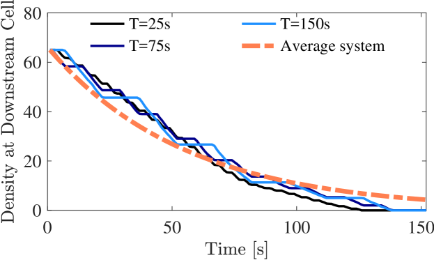
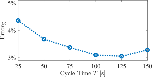
Figure 7: Accuracy of average dynamical model (5) with respect to microscopic simulations for a single signalized road. (a) Time evolution of the density at the downstream cell for different intersection cycle time $T$. (b) Inaccuracies of the average dynamics in relation to the intersection cycle time $T$.

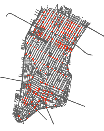
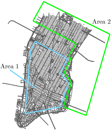
Figure 8: Geographic map of urban traffic interconnection in Manhattan. (a) Signalized intersections considered (red dots). (b) Commute areas considered.

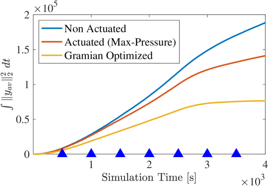
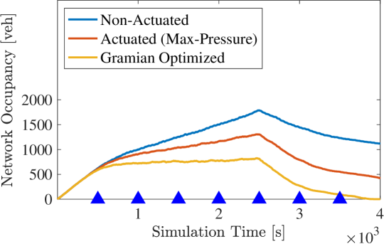
Figure 9: Network performance of the Manhattan urban interconnection assessed via a microscopic simulation for three control policies. Blue triangles denote the time instants where the solution to (III) is re-computed with updated $x_{0}$. (a) Cost of congestion associated with traffic signaling (see optimization (7)). (b) Total number of vehicles in the network.

V Simulations

This section provides numerical simulations in support to the assumptions made in this paper, and includes discussions and demonstrations of the benefits of our methods. We generate test cases using real-world traffic networks from the OpenStreet Map database and validate the techniques on a simulator based on Sumo (Simulation of Urban MObility [29]).

We first consider a single road, connected at downstream to a signalized intersection (e.g. Fig. 3), and illustrate in Fig.  7 a comparison between the trajectories of the switching system (4) and the trajectories of the average dynamical model (5). The figure shows the discharging pattern over time of the cell at road downstream, resulting from a microscopic simulation. In the simulation, the initial downstream cell density is $x^{\sigma}=65$veh and, for simplicity, there are no inflows to the road. Fig. 7 demonstrates the accuracy of the approximation for different choices of the split cycle time $T$. The precision of the model can be quantitatively assessed by considering the following error-measure over a certain time horizon $[0,\mathcal{H}]$:

$$\text{Error}_{\%}=\frac{1}{\mathcal{H}}\int_{0}^{\mathcal{H}}\frac{\|x-{x}_{\textup{av}}\|}{\|{x}_{\textup{av}}\|}~{}dt.$$ (15)

The relative error measure (15) captures the deviation of (5) from the microscopic simulation, normalized with respect to the road density and the considered time horizon. As indicated in Fig. 7, the inaccuracies due to linearization and time-averaging are under $5\%$ for common intersection cycle times.

TABLE I: Manhattan Network Inflow Rates

Time [sec]
(From - To)	Area 1 Inflow [veh/h]	Area 2 Inflow [veh/h]
$0-2500$	$4000$	$0$
$2500-4000$	$0$	$0$

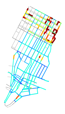
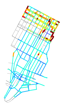
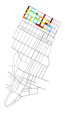
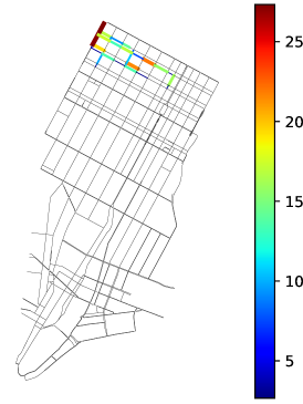
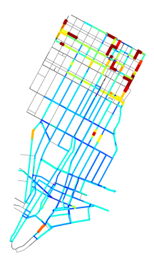
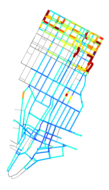
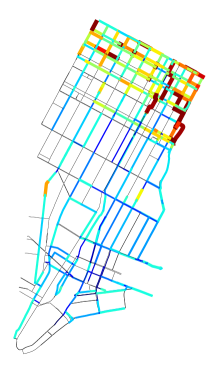
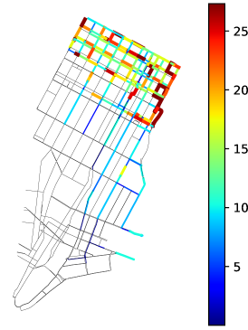
Figure 10: Time evolution of the network state (traffic density [veh/cell]) for: (a)-(d) solution to (7); (e)-(h) Max-Pressure policies. ((a) and (e)) $\text{simulation time}=1000$; ((b) and (f)) $\text{simulation time}=2000$; ((c) and (g)) $\text{simulation time}=3000$; ((d) and (h)) $\text{simulation time}=4000$. The comparison shows that the solution to (7) leads to faster traffic dynamics that results in reduced travel time.

We then consider a test case (Fig. 8) inspired by the area of Manhattan, NY, which features ${n}_{\textup{r}}=958$ roads and $n_{\mathcal{I}}=332$ signalized intersections. We replicate a daily-commute scenario, where sources of traffic flows $\mathcal{S}$ are uniformly distributed in the central area of the island (Area 1), and routing is chosen so that traffic flows are departing from the city, that is, destinations $\mathcal{D}$ are uniformly distributed within Area 2. Each vehicle follows the shortest path between its source-destination pair, and the discretization is performed with $h=0.1$ miles. The inflow-rates employed in the simulation are summarized in Table I. Fig. 9 shows a comparison, in terms of the cost function in (7), resulting from the microscopic simulation of: (i) an implementation of the optimal solution to (III), (ii) adaptive distributed control policies (Max-Pressure [2]), and (iii) fixed time control [12]. For scenario (i), the output of the optimization (III) is employed to construct feasible sets of phases at each intersection, where cycle time is set to $T=100$sec, and no optimization is performed to decide the specific sequence of phases at each intersection. Consequently to the argument presented in Section II-D, the solution to (III) is re-computed with updated traffic conditions (i.e. $x_{0}$) every $500$sec. Fig. 9 shows a comparison of the total number of vehicles in the network, for the three control techniques considered. As highlighted from the simulation, the availability of an overall network model, capable of capturing all the relevant network dynamics and dynamical interactions between diverse network components, results in reduced roads occupancy, which in turn implies improved network congestion, throughput, and vehicle travel time [23]. The effects of different control policies on the network overall congestion can be further visualized by means of the graphical illustration in Fig. 10. The figure shows the geographical displacement of traffic over time. The graphic highlights that the the possibility to estimate the network current traffic conditions, combined with optimization problems of the form (7), result in faster system responses against congestion, that ultimately result in shorter ”cool down“ phases. Notably, the network is evacuated faster as compared to techniques that rely on local knowledge of the traffic conditions. Finally, the above simulation (Fig. 10) also validates the argument presented in Section II-D, that is, when exogenous inflows are unknown, the current inflow demands enter the optimization through the initial state $x_{0}$, and motivates our formulation (7).

VI Conclusions

This paper describes a simplified model to capture in a tractable way the overall dynamics of urban traffic networks. This model allows us to reformulate the goal of optimizing network congestion as the problem of minimizing a metric of controllability of an appropriately defined dynamical system associated with the network. Our results show that the availability of an approximate model of the overall network can considerably improve the network efficiency, and allows for a more tractable analysis compared to traditional models. We show how the performance of other distributed policies deteriorate as compared to centralized models, due to the lack of availability of a global dynamical model capable of capturing all the relevant network dynamics. We adapt our technique to fit distributed and/or parallel implementations, and provide an efficient way to optimize large groups of intersections under the practical assumption that each agent has only local knowledge on the infrastructure. We envision that our model of traffic network and the proposed optimization framework will be useful in future research targeting design of traffic networks, control, and security analysis.

References

- [1] G. Bianchin, A Sumo interface for Gramian-Based traffic optimization, https://github.com/gianlucaBianchin/Gramian-Based-Traffic-Optimization, [Online] (2018).
- [2] P. Varaiya, The max-pressure controller for arbitrary networks of signalized intersections, in: Advances in Dynamic Network Modeling in Complex Transportation Systems, Springer, 2013, pp. 27–66.
- [3] C. Diakaki, M. Papageorgiou, K. Aboudolas, A multivariable regulator approach to traffic-responsive network-wide signal control, Control Engineering Practice 10 (2) (2002) 183–195.
- [4] E. Lovisari, G. Como, A. Rantzer, K. Savla, Stability analysis and control synthesis for dynamical transportation networks, arXiv preprint.
- [5] Q. Ba, K. Savla, G. Como, Distributed optimal equilibrium selection for traffic flow over networks, in: IEEE Conf. on Decision and Control, IEEE, 2015, pp. 6942–6947.
- [6] G. Gomes, Bandwidth maximization using vehicle arrival functions, IEEE Transactions on Intelligent Transportation Systems 16 (4).
- [7] S. Coogan, E. Kim, G. Gomes, M. Arcak, P. Varaiya, Offset optimization in signalized traffic networks via semidefinite relaxation, Transportation Research Part B: Methodological 100 (2017) 82–92.
- [8] P. Hunt, D. Robertson, R. Bretherton, M. C. Royle, The SCOOT on-line traffic signal optimisation technique, Traffic Engineering & Control 23 (4).
- [9] P. Mirchandani, L. Head, A real-time traffic signal control system: architecture, algorithms, and analysis, Transportation Research Part C: Emerging Technologies 9 (6) (2001) 415–432.
- [10] N. H. Gartner, F. J. Pooran, C. M. Andrews, Implementation of the opac adaptive control strategy in a traffic signal network, in: IEEE Transactions on Intelligent Transportation Systems, 2001, pp. 195–200.
- [11] T. Wongpiromsarn, T. Uthaicharoenpong, Y. Wang, E. Frazzoli, D. Wang, Distributed traffic signal control for maximum network throughput, in: IEEE Transactions on Intelligent Transportation Systems, 2012, pp. 588–595.
- [12] M. Papageorgiou, C. Diakaki, V. Dinopoulou, A. Kotsialos, Y. Wang, Review of road traffic control strategies, Proceedings of the IEEE 91 (12) (2003) 2043–2067.
- [13] K. Aboudolas, M. Papageorgiou, E. Kosmatopoulos, Store-and-forward based methods for the signal control problem in large-scale congested urban road networks, Transportation Research Part C: Emerging Technologies 17 (2) (2009) 163–174.
- [14] L. B. De Oliveira, E. Camponogara, Multi-agent model predictive control of signaling split in urban traffic networks, Transportation Research Part C: Emerging Technologies 18 (1).
- [15] C. Canudas-De-Wit, An average study of the signalized cell transmission model, [Online]. Available: https://hal.archives-ouvertes.fr/ hal-01635539/document.
- [16] P. Grandinetti, C. C. de Wit, F. Garin, Distributed optimal traffic lights design for large-scale urban networks, IEEE Transactions on Control Systems Technology (2018) 1–14doi:10.1109/TCST.2018.2807792.
- [17] J. Vanbiervliet, B. Vandereycken, W. Michiels, S. Vandewalle, M. Diehl, The smoothed spectral abscissa for robust stability optimization, SIAM Journal on Optimization 20 (1).
- [18] C. F. Daganzo, The cell transmission model: A dynamic representation of highway traffic consistent with the hydrodynamic theory, Transportation Research Part B: Methodological 28 (4).
- [19] M. Treiber, A. Kesting, Traffic flow dynamics, Traffic Flow Dynamics: Data, Models and Simulation, Springer-Verlag Berlin Heidelberg.
- [20] M. J. Lighthill, G. B. Whitham, On kinematic waves. ii. a theory of traffic flow on long crowded roads, Proceedings of the Royal Society of London. Series A, Mathematical and Physical Sciences (1955) 317–345.
- [21] R. E. Allsop, Delay-minimizing settings for fixed-time traffic signals at a single road junction, IMA Journal of Applied Mathematics 8 (2) (1971) 164–185.
- [22] R. Middlebrook, S. Cuk, A general unified approach to modelling switching-converter power stages, in: Power Electronics Specialists Conference, 1976, pp. 18–34.
- [23] G. Gomes, R. Horowitz, Optimal freeway ramp metering using the asymmetric cell transmission model, Transportation Research Part C: Emerging Technologies 14 (4) (2006) 244–262.
- [24] W. Xia, M. Cao, Analysis and applications of spectral properties of grounded laplacian matrices for directed networks, Automatica 80 (2017) 10–16.
- [25] D. G. Luenberger, Y. Ye, et al., Linear and nonlinear programming, Vol. 2, Springer, 1984.
- [26] R. H. Bartels, G. W. Stewart, Solution of the matrix equation AX+ XB= C, Communications of the ACM 15 (9).
- [27] F. Pasqualetti, R. Carli, F. Bullo, Distributed estimation via iterative projections with application to power network monitoring, Automatica 48 (5) (2012) 747–758.
- [28] S. Lämmer, D. Helbing, Self-control of traffic lights and vehicle flows in urban road networks, Journal of Statistical Mechanics: Theory and Experiment 2008 (04) (2008) P04019.
- [29] M. Behrisch, L. Bieker, J. Erdmann, D. Krajzewicz, Sumo - simulation of urban mobility: An overview, in: in SIMUL 2011, The Third International Conference on Advances in System Simulation, 2011, pp. 63–68.