Spectral modeling of type II supernovae

We present substantial extensions to the Monte Carlo radiative transfer code tardis to perform spectral synthesis for type II supernovae. By incorporating a non-LTE ionization and excitation treatment for hydrogen, a full account of free-free and bound-free processes, a self-consistent determination of the thermal state and by improving the handling of relativistic effects, the improved code version includes the necessary physics to perform spectral synthesis for type II supernovae to high precision as required for the reliable inference of supernova properties. We demonstrate the capabilities of the extended version of tardis by calculating synthetic spectra for the prototypical type II supernova SN1999em and by deriving a new and independent set of dilution factors for the expanding photosphere method. We have investigated in detail the dependence of the dilution factors on photospheric properties and, for the first time, on changes in metallicity. We also compare our results with two previously published sets of dilution factors by Eastman et al. (1996) and by Dessart & Hillier (2005a), and discuss the potential sources of the discrepancies between studies.

1 Introduction

In recent years the availability of spectral data for hydrogen-rich supernovae (Type II; SNe II) has increased dramatically. Measurements for hundreds of SNe II are now publicly accessible (see e.g., Poznanski et al. 2009; D’Andrea et al. 2010; Hicken et al. 2017, for recent data releases), providing a dataset that contains a wealth of information about the kinematics of the explosion, the progenitor systems (e.g., Jerkstrand et al. 2012), the circumstellar material (e.g., Quimby et al. 2007), and much more. Most of the analysis of this data has focused on the study of easily measurable spectral parameters such as line absorption velocities or equivalent widths and their correlations (see e.g., Gutiérrez et al. 2017b, a), omitting the full information contained in the spectra. To establish connections between these parameters and the underlying quantities, such as the metallicity, most studies rely on approximate relations that have been calibrated based on theoretical models (see e.g., Anderson et al. 2016). In contrast, only a few well-observed type II supernovae, such as SN1999em (Baron et al. 2004; Dessart & Hillier 2006), SN2005cs (Baron et al. 2007; Dessart et al. 2008) or SN2006bp (Dessart et al. 2008), have been studied using detailed radiative transfer models, which provide a direct way to infer information about the chemical composition, the density profile and other parameters from the full spectral time series. This applies in particular to the use of SNe II as distance indicators, despite the fact that an absolute distance estimate is a natural byproduct of a quantitative spectroscopic analysis (see Baron et al. 1995, 1996a, 2004, 2007; Lentz et al. 2001; Mitchell et al. 2002). SNe II have a long history as cosmological probes (Kirshner & Kwan 1974; Schmidt et al. 1994) and have regained popularity in recent years due to the increased availability of data at high redshifts (e.g., Poznanski et al. 2009; Gall et al. 2018) and, in the era of high precision cosmology, due to the rising need for independent tests of our cosmological models. Recent efforts have focused mainly on methods that rely on various observed correlations between photometric and spectroscopic parameters such as the standard candle method (SCM) by Hamuy & Pinto (2002), the photometric color method by de Jaeger et al. (2015) or the photospheric magnitude method by Rodriguez et al. (2014). Both Gall et al. (2018) and de Jaeger et al. (2017) demonstrate that with the SCM or the expanding photosphere method (EPM) distance measurements of SNe II up to redshifts of $\approx 0.34$ are feasible, highlighting the progress that has been made possible through the availability of new data. In contrast, the determination of distances from radiative transfer modeling has stagnated in recent years. Both the tailored EPM technique (Dessart & Hillier 2006; Dessart et al. 2008) and the spectral fitting expanding atmosphere method (SEAM) (Baron et al. 1995, 1996a, 2004, 2007) have never been applied outside the local universe. Nevertheless, their independence of the cosmic distance ladder as well as their foundation in well-understood physics make them a promising independent tool for cosmology.

Motivated by the wealth of available spectral data and the unique diagnostic abilities of radiative transfer modeling, we have developed a new numerical tool for performing spectroscopic analysis of SNe II. Since our main goal is to provide a tool for parameter inference, we neglect time-dependent effects in favor of computational expediency. Currently, the high computational costs prevent the application of numerical methods that self-consistently simulate the time evolution of the radiation field and the plasma state based on initial conditions (Dessart & Hillier 2011; Dessart et al. 2013) to this purpose. Our approach is an extension of the Monte Carlo radiative transfer code tardis (Kerzendorf & Sim 2014), which was originally developed for spectral synthesis in type Ia supernovae (SNe Ia). We have extensively modified and improved the physical treatment of radiative transfer implemented in tardis to be applicable to the modeling of SNe II atmospheres. This improved version of the code is then used to calculate a new, independent set of dilution factors for the EPM technique. In the EPM the dilution factors as introduced by Hershkowitz et al. (1986a, b) and Hershkowitz & Wagoner (1987) correct for the deviation of the supernova emission from that of a blackbody of the same color temperature. They provide the possibility to compare our model calculations to previously published numerical results by Eastman et al. (1996, E96 from now on) and Dessart & Hillier (2005a, D05 from now on) in a simple parametrized fashion. Currently, the systematic discrepancies between the two sets of dilution factors constitute one of the most significant sources of uncertainty in the EPM method, accounting for differences of roughly 20% in the inferred distance (e.g., Takats & Vinko 2006; Jones et al. 2009; Gall et al. 2016, 2018). This significant uncertainty highlights the need for additional calculations based on independent numerical methods to understand and resolve the current tension.

The structure of the paper is as follows. We begin with a detailed description of the physical extensions and their numerical implementation into tardis in Sect. 2. In Sect. 3, we provide a brief review of the EPM and discuss the basic physics of the dilution factors. As a first application of the extended version of tardis, we present radiative transfer models for two epochs of the prototypical SN II SN1999em in Sect. 4. The next sections are dedicated to the presentation and discussion of our main application, the calculation of a new set of EPM dilution factors. The setup of the necessary grid of supernova models is described in Sect. 5, followed by an analysis of the calculated dilution factors in Sect. 6. Here, we focus particularly on the differential influence of the model parameters such as photospheric density or metallicity. To put our results into context and to understand the differences between the published set of dilution factors, a comparison to previous studies is given in Sect. 7. We investigate the differences in the adopted numerical approaches and examine the different choices for the atmospheric properties. Finally, we summarize our results and give an outlook in Sect. 8.

2 Method

We present an extended version of the one-dimensional Monte Carlo (MC) radiative transfer code tardis (Kerzendorf & Sim 2014) that has been significantly extended for the application to SNe II. tardis is based on the indivisible energy packet MC methods of Lucy (1999a, b, 2002, 2003) and has been developed for rapid spectral modeling of SNe Ia. It has been used to study various aspects of SN Ia explosion physics. Applications include abundance tomographies (Barna et al. 2017), a study of spectral signatures of helium in double-detonation models (Boyle et al. 2017), as well as analyses of SNe Iax spectra (Magee et al. 2016, 2017). In these studies only the effects of Thomson scattering and bound-bound line interactions are simulated in detail. This is a reasonable approximation for SNe Ia but not for SNe IIP, which have a higher ratio of continuum to line opacity due to the hydrogen-rich composition. To adapt tardis to these conditions, we extend our treatment of radiation–matter interactions to include bound-free, free-free as well as collisional processes using the macro atom scheme of Lucy (2002, 2003) as outlined in Sect. 2.1. Further necessary improvements to the code can be motivated based on the peculiarities of radiative transfer in SNe II. SNe II atmospheres are characterized by comparatively low densities at the photosphere and a scattering dominated opacity. Due to the low densities, collisions are ineffective at coupling the level populations and ionization and excitation are mainly controlled by the radiation field. The radiation field is dilute compared to its equilibrium value as a result of the dominance of electron-scattering opacity and thus significant departures from local thermodynamic equilibrium (LTE) arise even far below the photosphere (see e.g., Dessart & Hillier 2011). To address this issue, we have extended the code as outlined in Sect. 2.2. Another consequence of the scattering dominated environment is that relatively high optical depths on the order of $\tau\propto\mathcal{O}(10)$ are needed to guarantee a full thermalization of the radiation (see e.g., Eastman et al. 1996). At such high optical depths the atmospheric structure is strongly affected by relativistic transfer effects as demonstrated by Hauschildt et al. (1991). The inclusion of these effect in tardis is described in Sect. 2.1.4.

2.1 Monte Carlo simulations

To find a consistent solution for the plasma state and the radiation field, tardis performs a series of Monte Carlo radiative transfer simulations. At every radiative transfer step, a large ensemble of indivisible energy packets (see Abbott & Lucy 1985; Lucy 1999a, 2002, 2003) representing monochromatic photon bundles is initialized at the inner boundary. Initial packet properties are assigned under the assumptions of the LTE diffusion limit. Thus, packet frequencies are sampled from a blackbody distribution at the inner boundary temperature $T_{\mathrm{i}}$ and propagation directions are selected according to zero limb-darkening in the comoving frame. Uniform packet energies are chosen such that the injected packets carry a total comoving frame luminosity $L_{\mathrm{i}}=4\pi R_{\mathrm{i}}^{2}\sigma T_{\mathrm{i}}^{4}$, where $\sigma$ is the Stefan-Boltzmann constant and $R_{\mathrm{i}}$ is the radius of the inner boundary. With initial properties assigned, the propagation of the packets is simulated under the assumption of a steady-state, that is to say, neglecting time dependence, as outlined in the following section.

2.1.1 Packet propagation

After initialization, each packet is followed until it leaves the computational domain through the inner or outer boundary. Between the boundaries the supernova atmosphere has been discretized into equidistant, spherical shells. Within each shell the plasma properties such as the opacity or the electron temperature are assumed to be constant. During the propagation the effects of Thomson scattering, hydrogen bound-free, free-free, bound-bound as well as collisional processes are taken into account. As described in Kerzendorf & Sim (2014), line opacity is treated in the Sobolev approximation (see Sobolev 1957). For micro-turbulent velocities on the order of $100\text{\,}\mathrm{km}\text{\,}{\mathrm{s}}^{-1}$, this is as accurate as the comoving frame method in describing the formation of the Balmer lines in SNe IIP (see Duschinger et al. 1995). Following Lucy (2003), the free-free opacity

$$\chi_{\mathrm{ff}}(\nu)=\alpha_{\mathrm{ff}}\,\nu^{-3}T_{\mathrm{e}}^{-1/2}n_{\mathrm{e}}\left(1-e^{-h\nu/k_{\mathrm{B}}T_{\mathrm{e}}}\right)\sum_{j,k}N_{j,k}(j-1)^{2}$$ (1)

is evaluated with free-free gaunt factors set to unity. Here, $N_{j,k}$ denotes the number density of ionization stage $j$ of element $k$, $T_{\mathrm{e}}$ is the electron temperature, $n_{\mathrm{e}}$ the electron density and $\nu$ the frequency. The prefactor $\alpha_{\mathrm{ff}}$ has the value $3.69\text{\times}{10}^{8}\text{\,}\mathrm{c}\mathrm{m}^{5}\mathrm{K}^{1/2}\mathrm{/}\mathrm{s}^{3}$. Since hydrogen is the dominant source of bound-free opacity in SNe II, we restrict the inclusion of these processes currently only to this element. However, since an extension to more species is conceptually straightforward, we present the governing equations in their general form. Thus, the opacity resulting from photoionizations of electrons in level $i$ of ion $j,k$ is given by

$$\chi_{i,j,k}^{\mathrm{bf}}(\nu)=\alpha_{i,j,k\rightarrow j+1,k}(\nu)\left(n_{i,j,k}-n_{i,j,k}^{*}e^{-h\nu/k_{\mathrm{B}}T_{\mathrm{e}}}\right),$$ (2)

where $n_{i,j,k}$ and $n_{i,j,k}^{*}$ denote the actual and the respective LTE level number densities (see equation 5.25 of Hubeny & Mihalas 2014). The cross-section for photoionzation $\alpha_{i,j,k\rightarrow j+1,k}(\nu)$ is obtained from tabulated values through linear interpolation.

To account for the inclusion of hydrogen bound-free, free-free as well as collisional processes small modifications to the packet propagation procedure of Kerzendorf & Sim (2014, §2.6) have been necessary. In particular for continuum interactions an additional MC experiment is needed to determine the physical absorption mechanism. The probabilities for bound- free absorption, free-free absorption and Thomson scattering are given by $\chi^{\mathrm{bf}}/(\chi^{\mathrm{bf}}+\chi^{\mathrm{ff}}+\chi^{\mathrm{Th}})$, $\chi^{\mathrm{ff}}/(\chi^{\mathrm{bf}}+\chi^{\mathrm{ff}}+\chi^{\mathrm{Th}})$ and $\chi^{\mathrm{Th}}/(\chi^{\mathrm{bf}}+\chi^{\mathrm{ff}}+\chi^{\mathrm{Th}})$ respectively. If a bound-free process is selected, a specific continuum for absorption has to be assigned according to the probabilities $\chi^{\mathrm{bf}}_{i,j,k}/\chi^{\mathrm{bf}}$ for photoionization from specific levels $i$ of ion $j,k$. Regardless of the type of interaction, we use the macro atom scheme of Lucy (2002, 2003) to select an emission channel as outlined in Sect. 2.1.2. For bound-free and free-free emission, the packet has to be assigned an appropriate frequency before the propagation can be resumed. We employ the approximate sampling rule of Lucy (2003, Eq. 41) for free-free processes and linear interpolation on precomputed values of the emissivity for bound-free interactions.

2.1.2 Macro atom

We use the macro atom scheme of Lucy (2002, 2003) for a general treatment of complicated radiation-matter interactions, such as recombination cascades, fluorescent line emission or cooling emission. In this scheme, packet splitting for processes with multiple emission channels is avoided by assigning the total energy of the packet randomly to one possible interaction channel according to a set of rules derived from the assumption of statistical equilibrium. In Kerzendorf & Sim (2014), only the redistribution of excitation energy created by bound-bound absorption events was simulated using the macro atom machinery. We introduce indivisible packets of thermal kinetic energy ($k$- packets) and ionization energy ($i$-packets) in addition to the packets of excitation energy (macro atoms) included in Kerzendorf & Sim (2014) to treat continuum interactions. $k$-packets can be created by bound-free and free-free absorption events as well as collisional deactivations of $i$-packets or macro atoms. Since both thermal and ionization energy are created in photoabsorption events, the $r$-packet is transformed into a $k$-packet with probability $p^{k}=\nu_{i,j,k}/\nu^{\prime}$ and into an $i$-packet otherwise. Here, $\nu_{i,j,k}$ is the threshold for ionization and $\nu^{\prime}$ is the frequency of the $r$-packet in the comoving frame. Based on the assumption of radiative balance in the fluid rest frame, all $i$-packets, macro atoms and $k$-packets have to be converted in-situ back to $r$-packets. For $k$-packets this is done by sampling the rates at which different physical processes cool the electron gas. All treated cooling rates are listed in Sect. 2.2.3. For macro atoms and $i$-packets, the situation is more complicated due to the possibility of internal transitions. In both cases we sample the internal energy flow rates until a radiative deexcitaton process is selected or a collisional deactivation to a $k$-packet occurs (see Lucy 2002, 2003). The needed energy flow rates are calculated with rate coefficients evaluated as described in Sect. 2.2.

2.1.3 Reconstruction of radiation field quantities

For our detailed treatment of ionization and thermal structure (see Sect. 2.2), estimates for the radiative bound-free rates and radiative heating rates are needed. We use volume-based estimators (Lucy 1999b, 2003) to reconstruct the relevant quantities from the trajectories of the packet ensemble. In this approach, the time-averaged contributions of all trajectory segments, on which the process can in principle occur, are taken into account. Thus, to obtain an estimate for the photoionization rate coefficient $\gamma_{i,j,k}$ for level $i,j,k$, we sum over all path segments $\mathop{}\!\mathrm{d}{s}$ for which the comoving frame (CMF) frequency $\nu^{\prime}$ of the packet is larger than the threshold for photoionization $\nu_{i,j,k}$

$$\gamma_{i,j,k}=\frac{1}{\Delta tV}\sum_{\nu^{\prime}\geq\nu_{i,j,k}}\varepsilon^{\prime}_{\nu}\frac{\alpha_{i,j,k\rightarrow j+1,k}(\nu^{\prime})}{h\nu^{\prime}}\mathop{}\!\mathrm{d}{s}.$$ (3)

Here, $V$ is the volume of the respective grid cell and $\varepsilon^{\prime}_{\nu}$ is the CMF packet energy. The time interval $\Delta t$ is a numerical normalization factor that is determined by the energy injection rate at the lower computational boundary. Similarly, the estimator for the stimulated recombination rate coefficient is given by

$$\alpha_{i,j,k}^{\mathrm{stim}}=\Phi_{i,j,k}(T_{\mathrm{e}})\frac{1}{\Delta tV}\sum_{\nu^{\prime}\geq\nu_{i,j,k}}\epsilon^{\prime}_{\nu}\frac{\alpha_{i,j,k\rightarrow j+1,k}(\nu^{\prime})}{h\nu^{\prime}}e^{-h\nu^{\prime}/k_{\mathrm{B}}T_{\mathrm{e}}}\mathop{}\!\mathrm{d}{s}.$$ (4)

Here, the Saha factor

$$\Phi_{i,j,k}(T)=\frac{n_{i,j,k}^{*}}{n_{0,j+1,k}^{*}n_{\mathrm{e}}}$$ (5)

enters, which connects the LTE level populations $n_{i,j,k}^{*}$ to the ground state population $n_{0,j+1,k}^{*}$ of the next higher ionization stage. The heating rate coefficient for photoionization is

$$h^{\mathrm{bf}}_{i,j,k}=\frac{1}{\Delta tV}\sum_{\nu^{\prime}\geq\nu_{i,j,k}}\varepsilon^{\prime}_{\nu}\alpha_{i,j,k\rightarrow j+1,k}(\nu^{\prime})\left(1-\frac{\nu_{i,j,k}}{\nu^{\prime}}\right)\mathop{}\!\mathrm{d}{s}.$$ (6)

Finally, the heating rate $H^{\mathrm{ff}}$ due to inverse-bremsstrahlung is calculated using

$$H^{\mathrm{ff}}=\frac{1}{\Delta tV}\sum\chi_{\mathrm{ff}}(\nu)\epsilon^{\prime}_{\nu}\mathop{}\!\mathrm{d}{s},$$ (7)

with the free-free opacity $\chi_{\mathrm{ff}}(\nu)$ treated according to Eq. 1. Before concluding our presentation of the reconstruction of radiation field quantities, we stress again that currently the estimators for the bound-free processes $\gamma_{i,j,k}$, $\alpha_{i,j,k}^{\mathrm{stim}}$ and $h^{\mathrm{bf}}_{i,j,k}$ are only used for hydrogen.

2.1.4 Relativistic transfer

For photospheric-phase SNe II the emergent continuum radiation is created in regions well below the photosphere. In these optically thick regions, the radiation field is essentially isotropic in the fluid rest frame and relativistic frame transformations can significantly modify the energy transport in the ejecta by introducing small anisotropies in the lab frame intensity (see e.g., Hauschildt et al. 1991; Baron et al. 1996b).

To include relativistic effects in the Monte Carlo simulations, tardis uses a mixed-frame approach. Radiation–matter interactions are handled in the comoving frame whereas the packet propagation is carried out in the lab frame. Whenever necessary we transform the relevant packet properties between the frames. Compared to Kerzendorf & Sim (2014), we have refined the treatment of relativity by including frame transformations of opacities as well as angle aberration. To transform packet energies and frequencies between observer and comoving frame, we use the full Doppler factor instead of an first order approximation. Expressions for the relevant transformations laws can be found in Mihalas & Mihalas (1984) or, specifically for spherical geometries, in Castor (1972). To be consistent with the adopted frame transformations, the distance to the next possible line interaction is now calculated based on the full Doppler-shift formula. As a result, the common-direction frequency surfaces, that is, the surfaces that emit line radiation at the same frequency in the observer frame, are no longer planes perpendicular to the line of sight but have a more complicated geometry as described by the relativistic Sobolev theory of Jeffery (1995).

2.2 Plasma state

The original implementation of tardis only features approximate excitation and ionization treatments and a very simplified calculation of the thermal structure. We have considerably refined the determination of the plasma state to adapt the code to SNe II. In particular, we have implemented a full NLTE treatment of excitation and ionization for hydrogen and we employ a thermal balance calculation to infer the temperature structure of the envelope.

The calculation of the plasma state involves a simultaneous determination of the excitation and ionization state of the material as well as the thermal structure. To reduce the complexity of this nonlinear problem, we decouple the solution of the excitation and ionization balance as follows: given an initial guess for the kinetic temperature $T_{\mathrm{e}}$ and the electron density $n_{\mathrm{e}}$, we calculate level population fractions as outlined in Sect. 2.2.1. Based on the obtained excitation state, we solve for the ionization balance as described in Sect. 2.2.2. Finally, we compute heating and cooling rates (see Sect. 2.2.3), which are needed for the determination of the thermal structure. An outer iteration loop establishes consistency between excitation and ionization and adjusts the temperature such that thermal balance is enforced (see Sect. 2.2.4).

2.2.1 Excitation

tardis offers excitation treatments with different levels of sophistication. Level population fractions $f_{i,j,k}=n_{i,j,k}/N_{j,k}$ can be calculated from the Boltzmann excitation equation, a nebular modification thereof (see Abbott & Lucy 1985) or from the steady-state equations of statistical equilibrium.

For the NLTE excitation calculation, electron number densities have to be specified. In this case, the statistical equilibrium equations for the total system decouple and can be solved for each atomic species individually. In the NLTE treatment of Kerzendorf & Sim (2014), only bound-bound interactions and collisional excitation and deexcitation rates were included. We extend the scheme by including radiative and collisional bound-free processes to obtain a more complete description of hydrogen excitation. The necessary photoionization and recombination rate coefficients $\gamma_{i}$ and $\alpha_{i}$ are reconstructed from the MC simulation by volume- based estimators (see Sect. 2.1.3). The collisional ionization and recombination rate coefficients $q_{i\kappa}$ and $q_{\kappa i}$ are evaluated according to the approximate formula by Seaton (1962). With these processes included, the rate equation for level $i$ of ion $j,k$ is given by

$$-\left(\gamma_{i}+q_{i\kappa}n_{\mathrm{e}}+\sum_{m\neq i}r_{im}\right)f_{i}+\sum_{m\neq i}r_{mi}f_{m}=-(\alpha_{i}+q_{\kappa i}n_{\mathrm{e}})\frac{N_{j+1,k}n_{\mathrm{e}}}{N_{j,k}}.$$ (8)

Here, $r_{mi}$ and $r_{im}$ denote the total rate coefficients at which radiative and collisional transitions between level $i$ and $m$ populate and depopulate level $i$. In the Sobolev approximation, the rate coefficient for deexcitation from an upper level $u$ to a lower level $l$ is given by

$$r_{ul}=\beta_{lu}A_{ul}+\beta_{lu}B_{ul}J^{\mathrm{b}}_{lu}+c_{ul}n_{\mathrm{e}}$$ (9)

and the excitation rate coefficient is

$$r_{lu}=\beta_{lu}B_{lu}J^{\mathrm{b}}_{lu}+c_{lu}n_{\mathrm{e}}.$$ (10)

Here, $J^{\mathrm{b}}_{lu}$ is the mean intensity at the blue wing of the line, $\beta_{lu}$ is the Sobolev escape probability (see e.g., §4.3.1 of Lucy 2002) and $A_{lu},B_{lu}$ and $B_{ul}$ are the Einstein coefficients. Electron impact excitation rate coefficients $c_{lu}$ are taken from the approximate formula of van Regemorter (1962) with deexcitation rates evaluated according to detailed balance. For hydrogen levels with principal quantum numbers up to $n=7$ we use collision strengths from the detailed ab initio calculations of Przybilla & Butler (2004).

Despite fixing the electron number densities, the system of rates equations 8 remains nonlinear due to the dependence of the Sobolev escape probabilities on the level populations. We use a standard root finding algorithm to solve for the level population fractions $f_{i,j,k}=n_{i,j,k}/N_{j,k}$ and the ion population ratio $N_{j+1,k}/N_{j,k}$. The convergence of the outer iteration loop that establishes a consistent plasma state is accelerated considerably by including the ion population ratio in the solution of the excitation state.

2.2.2 Ionization

In our detailed treatment of ionization we use the derived level population fractions $n_{i,j,k}/N_{j,k}$ and an initial guess for the electron density $n_{\mathrm{e}}$ to calculate the total ionization rate coefficient

$$\Gamma_{j,k}=\sum_{i}n_{i,j,k}(q_{i,j,k\rightarrow j+1,k}n_{\mathrm{e}}+\gamma_{i,j,k})/N_{j,k}$$ (11)

and the total recombination rate coefficient

$$\alpha_{j+1,k}=\sum_{i}\left(\alpha^{\mathrm{sp}}_{i,j,k}+\alpha^{\mathrm{stim}}_{i,j,k}+q_{i,j,k\leftarrow j+1,k}n_{\mathrm{e}}\right)$$ (12)

for relevant pairs of ions $(j,k)$, $(j+1,k)$. We only do this for hydrogen in this work. For all other ions, the Saha factor $\Phi_{j,k}=(N_{j+1,k}n_{\mathrm{e}})/N_{j,k}$ and the electron density $n_{\mathrm{e}}$ serve as approximations of the total ionization and recombination rate coefficients. The Saha factor $\Phi_{j,k}$ is evaluated according to the Saha equation at the local radiation temperature $T_{\mathrm{R}}$ or the nebular ionization formula of Mazzali & Lucy (1993) (see Eqs. 2 and 3 of Kerzendorf & Sim 2014). Based on these ionization and recombination rate coefficients, we iteratively solve for the ion and electron number densities, assuming ionization equilibrium.

2.2.3 Thermal balance

To complete the description of the plasma state, we need an estimate for the electron temperature $T_{\mathrm{e}}$ in the ejecta. In Kerzendorf & Sim (2014), $T_{\mathrm{e}}$ was set to $0.9T_{\mathrm{R}}$ following Mazzali & Lucy (1993). We replace this simplified treatment of the thermal structure by a thermal-balance calculation based on the heating and cooling rates of the gas.

The thermal energy content, and therefore the temperature, is determined by the energy exchange between the kinetic energy of the ejecta, the radiative energy pool and the pool of atomic internal energy. This transfer is mediated by adiabatic cooling, collisional transitions as well as bound-free and free-free interactions. Assuming a steady-state, the rates for heating and cooling of the ejecta by these processes must cancel. Thus the electron temperature $T_{\mathrm{e}}$ is fixed by the requirement of thermal balance

$$H^{\mathrm{bf}}+H^{\mathrm{ff}}+H^{\mathrm{deexc}}+H^{\mathrm{recomb}}=C^{\mathrm{fb}}+C^{\mathrm{exc}}+C^{\mathrm{ion}}+C^{\mathrm{ad}}+C^{\mathrm{ff}}.$$ (13)

Here, $H^{\mathrm{bf}}$ and $C^{\mathrm{fb}}$ denote the rates of heating and cooling by bound-free interactions, $H^{\mathrm{ff}}$ and $C^{\mathrm{ff}}$ the respective rates for free-free processes. The contributions from collisional excitation, deexcitation, ionization and recombination are $C^{\mathrm{exc}}$, $H^{\mathrm{deexc}}$, $C^{\mathrm{ion}}$ and $H^{\mathrm{recomb}}$. The final term $C^{\mathrm{ad}}$ describes adiabatic cooling of the envelope due to expansion work.

Specifically, collisional excitations from lower levels $l,j,k$ to level $i,j,k$ remove energy from the thermal pool with a rate

$$C_{i,j,k}^{\mathrm{exc}}=\sum_{l}C_{l,j,k\rightarrow i,j,k}(\epsilon_{i,j,k}-\epsilon_{l,j,k}),$$ (14)

where $\epsilon_{i,j,k}$ and $\epsilon_{l,j,k}$ are the respective level energies. Correspondingly, collisional ionizations from bound levels of ion $j,k$ contribute

$$C_{j+1,k}^{\mathrm{ion}}=\sum_{l}C_{l,j,k\rightarrow j+1,k}(\epsilon_{0,j+1,k}-\epsilon_{l,j,k})$$ (15)

to the total cooling rate.

In turn, atomic internal energy is transfered to the thermal pool by the inverse processes of collisional recombination and deexcitation at rates

$$H_{j,k}^{\mathrm{recomb}}=\sum_{l}C_{l,j,k\leftarrow j+1,k}(\epsilon_{0,j+1,k}-\epsilon_{l,j,k})$$ (16)

and

$$H_{i,j,k}^{\mathrm{deexc}}=\sum_{u}C_{i,j,k\leftarrow u,j,k}(\epsilon_{u,j,k}-\epsilon_{i,j,k}).$$ (17)

Thermal electrons moving in the field of an ion $j,k$ emit radiative energy according to (see Osterbrock 1974)

$$C_{j,k}^{\mathrm{ff}}=$1.426\text{\times}{10}^{-27}\text{\,}\mathrm{(}$j-1)^{2}T_{\mathrm{e}}^{1/2}N_{j,k}n_{\mathrm{e}},$$ (18)

which depends on the ionic charge $j-1$, the number density of the respective ion $N_{j,k}$ as well as $T_{\mathrm{e}}$ and $n_{\mathrm{e}}$. In addition, energy is continuously removed from the thermal electron pool by radiative recombinations. In terms of the modified rate coefficient

$$\alpha_{i,j,k}^{\mathrm{E,sp}}=4\pi\,\Phi_{i,j,k}(T_{\mathrm{e}})\int_{\nu_{i,j,k}}^{\infty}\frac{\alpha_{i,j,k\rightarrow j+1,k}(\nu)}{h\nu_{i,j,k}}\frac{2h\nu^{3}}{c^{2}}e^{-h\nu/k_{\mathrm{B}}T_{\mathrm{e}}}\mathop{}\!\mathrm{d}{\nu}$$ (19)

the cooling rate by recombinations to level $i,j,k$ can be written as

$$C_{i,j,k}^{\mathrm{fb,sp}}=N_{j+1,k}n_{\mathrm{e}}\left(\alpha_{i,j,k}^{\mathrm{E,sp}}-\alpha_{i,j,k}^{\mathrm{sp}}\right)h\nu_{i,j,k}.$$ (20)

Photoionizations, in turn, heat the medium with a rate

$$H_{i,j,k}^{\mathrm{bf}}=4\pi n_{i,j,k}\int_{\nu_{i,j,k}}^{\infty}\alpha_{i,j,k\rightarrow j+1,k}(\nu)\left(1-\frac{\nu_{i,j,k}}{\nu}\right)J_{\nu}\mathop{}\!\mathrm{d}{\nu}.$$ (21)

Finally, the electron gas continuously loses thermal kinetic due to the expansion of the ejecta. The rate of energy loss resulting from this adiabatic cooling is given by

$$C^{\mathrm{ad}}=3n_{\mathrm{e}}k_{\mathrm{B}}T_{\mathrm{e}}/t,$$ (22)

where $t$ denotes the time of explosion.

2.2.4 Outer plasma iteration

To obtain a consistent solution for the plasma state, the input electron densities that are used in the calculation of the level population fractions have to agree with the results from the ionization calculation. This is achieved by combining the methods described above with an iterative root-finding procedure. Apart from establishing consistency between the excitation and ionization state, the outer iteration loop is used to determine the thermal structure from the thermal balance equation 13.

2.3 Approximations

As established by Utrobin & Chugai (2005); Dessart & Hillier (2007, 2010); Potashov et al. (2017) time-dependent effects in the excitation and ionization balance can play an important role in shaping the spectral energy distribution. This applies in particular to epochs following hydrogen recombination. At these times the inclusion of time-dependent terms induces an overionization compared to the steady state solution, which is crucial in reproducing the observed H$\alpha$ line strengths. In contrast, for epochs preceding hydrogen recombination the influence of time dependence is modest. Since these epochs are most relevant for the application of EPM (see e.g., Dessart & Hillier 2006; Dessart et al. 2008), we do not consider our neglect of these effects a severe limitation to our approach. In fact, Dessart & Hillier (2007) find negligible differences between the dilution factors from their time-dependent calculations and the steady-state results from Dessart & Hillier (2006); Dessart et al. (2008). Only for color temperatures less than $7000\text{\,}\mathrm{K}$ the correction factors drop systematically below their steady-state counterparts. As an additional approximation in the solution of the statistical equilibrium equations, we assume detailed radiative balance in the Lyman continuum. This prevents MC noise in the estimator for the ground- state photoionization rate from hindering convergence and avoids associated fluctuations in the ionization as well as the heating and cooling balance. This approach follows previous studies of SNe IIP, such as Takeda (1990, 1991) and Duschinger et al. (1995). Since the Lyman continuum is optically thick as long as the outflow ionization is not extremely high, detailed balance is deemed to be a very good approximation under most conditions of interest. We have verified this by a series of test calculations without this assumption but with increased numbers of MC quanta. The spectra resulting from the two approaches show good agreement for the parameter space that has been investigated in this paper. This is consistent with the results of Duschinger et al. (1995) who have reached the same conclusion for pure hydrogen supernova atmospheres with photospheric temperatures up to $15\,000\text{\,}\mathrm{K}$.

2.4 Iteration cycle

Tardis alternates between the calculation of the plasma state and MC radiative steps to achieve a self-consistent state for radiation and matter. Generally, less than twenty of these iterations are needed to achieve convergence to a point where only statistical variations remain (see Fig. 1). The good convergence properties result from the strict enforcement of radiative equilibrium, the explicit treatment of scattering and the direct dependence of the macro atom emissivities on the current estimate of the radiation field through the macro atom activation rates. At the moment, the number of iterations is set by hand at the beginning of the simulation, since no formal convergence criterion is implemented in Tardis. For the calculations presented in this paper, we have performed 40 iterations in all cases. We have found this to be more than sufficient to guarantee convergence for all used setups.

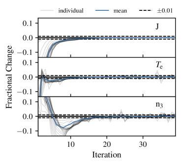
Figure 1: Illustration of the convergence properties of plasma and radiation field quantities. We show the fractional changes between successive iterations for the mean intensity of the radiation field $J$, the electron temperature $T_{\mathrm{e}}$ and a representative level population, specifically that of the second excited level of hydrogen $n_{3}$. In all cases, we include both the changes in each individual shell (gray) as well as their average (blue). The results shown here are taken from our SN1999em model for the 14th of November (see Sect. 4 and Fig. 3).

2.5 Atomic data

We use the hydrogen atomic data as described by Sim et al. (2005). This data set is based on a 20 level model atom with each level corresponding to a principal quantum number $n$. Frequency-dependent photoionization cross sections are tabulated for every energy state. The tabulated values range from the threshold ionization frequency up to the point at which the cross-section is only about $0.07\text{\,}\mathrm{\char 37\relax}$ of the value at threshold. This improved hydrogen model atom complements the atomic data already included in tardis (see Kerzendorf & Sim 2014), which is compiled from the line lists of Kurucz & Bell (1995) and the Chianti 7.1 data base (Dere et al. 1997; Landi et al. 2012).

2.6 Spectral synthesis

To calculate synthetic spectra, the properties of escaping packets are recorded and later binned. However, the quality of the spectra that can be obtained from the normal MC quanta is severely affected by MC noise. To improve the signal-to-noise ratio an additional type of MC packet is used in tardis. Whenever a normal packet is launched or performs an interaction in the final spectral synthesis run, these so called “virtual” packets ($v$-packets) are emitted to estimate the contribution of the event to the emergent spectrum. In practice this amounts to optical depth integrations along a number of randomly selected trajectories through the ejecta. The measured optical depths $\tau_{\mathrm{trj}}$ are then used to weight the contributions of the virtual packets to the spectrum according to the escape probability along the packet path, $\exp(-\tau_{\mathrm{trj}})$. This procedure, commonly called “peeling off”, is well established and has found widespread use, in particular in the area of dust MC radiative transfer (see e.g., Yusef-Zadeh et al. 1984; Wood & Reynolds 1999; Baes et al. 2011; Steinacker et al. 2013; Lee et al. 2017).

Compared to the implementation described in Kerzendorf & Sim (2014), modifications have been necessary to keep the computational effort reasonable for the high optical depths of our SN II atmospheres. Since the number of interactions scales quadratically with optical depth, the number of virtual packets that have to be tracked for each “real” packet quickly becomes prohibitively large as the optical depth is increased. At the same time, the contribution of the additional $v$-packets to the spectrum is marginal due to the strong attenuation towards the surface. We apply biasing to the virtual packet emission to tackle this issue. Virtual packets are created only with a probability $\exp(-\tau_{\mathrm{e}})$, where $\tau_{\mathrm{e}}$ is the electron scattering optical depth. To account for the lower chance of creation, the weight of the spawned packet is increased by the inverse of this probability. Notwithstanding this application of biasing, virtual packets can still accumulate large amounts of optical depth, for example in line interactions. We use the Russian roulette technique (see e.g., Carter & Cashwell 1975; Dupree & Fraley 2002) to probabilistically remove these low-weight packets.

2.7 Supernova model

tardis allows for the use of complex supernova models based on hydrodynamical explosion simulations and with stratified abundances (see Kerzendorf & Sim 2014, Appendix A). Nevertheless, to facilitate the exploration of the parameter space, we restrict our analysis to simple, highly parameterized models. As in D05, we assume power- law density profiles

$$\rho(r)=\rho_{0}(r/r_{0})^{-n}$$ (23)

with density indexes $n=-\mathop{}\!\mathrm{d}{\ln{\rho}}/\mathop{}\!\mathrm{d}{\ln{r}}$ in the range $n=6-14$. Both hydrodynamic simulations (Chevalier 1976, 1982; Blinnikov et al. 2000) and spectral modeling (see e.g., Eastman & Kirshner 1989; Schmutz et al. 1990; Baron et al. 2007; Dessart & Hillier 2006; Dessart et al. 2008) have demonstrated that the outer density distribution is well described by such an ansatz with values close to $n\sim 10$. The composition of the ejecta is taken to be homogeneous. Heavy elements up to nickel are included in the simulations. Following D05 we use CNO-cycle equilibrium values from Prantzos et al. (1986) for the abundances of H, He, C, N, O. The remaining elements are assumed to have solar chemical composition with values taken from Asplund et al. (2009).

3 Expanding photosphere method

3.1 Presentation of the method

The expanding photosphere method (EPM) of Kirshner & Kwan (1974) is based on a simplified model of the supernova as a sharply-defined, spherically-symmetric, expanding photosphere. The radiation emerging from this photosphere is assumed to be that of a blackbody, diluted by an amount given by the dilution factor $\xi_{\nu}$. This correction factor $\xi_{\nu}$ has originally been introduced by Hershkowitz et al. (1986a, b) and Hershkowitz & Wagoner (1987) to correct for the dilution of continuum flux that occurs in a scattering-dominated environment. In practice, the dilution factors account for all deviations of the spectrum from blackbody emission, such as lines or limb-darkening, in a parametrized fashion (see e.g., ; , ). For reasons of simplicity, in the application of EPM it is assumed that the dilution factor only depends on the color temperature. The precise form of this dependence may be reconstructed from supernovae whose distance is known from independent means (see Schmidt et al. 1992). However, to determine absolute distances it is necessary to infer the dilution factors from theoretical models as in E96 and D05, and outlined at the end of this section.

Based on the assumptions given above, the specific luminosity of the supernova is given by

$$L_{\nu}=4\pi\xi_{\nu}^{2}R_{\mathrm{ph}}^{2}\pi B_{\nu}(T),$$ (24)

where $R_{\mathrm{ph}}$ is the photospheric radius and $T$ is the temperature of the blackbody $B_{\nu}(T)$. By equating this to the observed de-reddened luminosity $L_{\nu}^{\mathrm{obs}}=4\pi D^{2}f_{\nu}^{\mathrm{dered}}$ the angular size of the expanding photosphere

$$\theta=\frac{2R_{\mathrm{ph}}}{D}=2\,\,\sqrt[]{\frac{f_{\nu}^{\mathrm{dered}}}{\xi_{\nu}^{2}\pi B_{\nu}(T)}}$$ (25)

can be inferred from the measured de-reddened flux $f_{\nu}^{\mathrm{dered}}$. The temperature $T$ has to be determined from photometry as will be outlined shortly. Finally, to obtain the distance to the supernova

$$D=\frac{2R_{\mathrm{ph}}}{\theta},$$ (26)

the photospheric radius must be eliminated from the equations. For homologous expansion this can be achieved via the relation

$$R_{\mathrm{ph}}=v_{\mathrm{ph}}(t-t_{0}),$$ (27)

where $t_{0}$ is the time of explosion and $v_{\mathrm{ph}}$ is the photospheric velocity. The expansion velocity $v_{\mathrm{ph}}$ can be inferred from blueshift velocities of lines, from cross-correlation of the observations with model spectra (see Hamuy et al. 2001) or from tailored radiative transfer calculations (see e.g., Dessart & Hillier 2006; Dessart et al. 2008). Finally, by measuring the ratio of photospheric angular diameter and velocity

$$\frac{\theta}{v_{\mathrm{ph}}}=\frac{t-t_{0}}{D}$$ (28)

for multiple epochs $t$, the distance is obtained from the slope of the data points. The time of explosion follows from the intercept with the $t$- axis.

To apply this formalism to observations, we have to recast the relevant equations in terms of photometric magnitudes. For a bandpass $\bar{\nu}$ with a transmission function $\phi_{\bar{\nu},\nu}$ the apparent magnitude $m_{\bar{\nu}}$ of the object can be calculated from the observed flux $f_{\nu}^{\mathrm{obs}}$ according to

$$m_{\bar{\nu}}=-2.5\log\left(\int_{0}^{\infty}\mathop{}\!\mathrm{d}{\nu}\phi_{\bar{\nu},\nu}f_{\nu}^{\mathrm{obs}}\right)+C_{\bar{\nu}},$$ (29)

where $C_{\bar{\nu}}$ is the zero-point. Using this definition, we can rewrite Eq. 24 for the dilute-blackbody emission as follows:

$$m_{\bar{\nu}}=-5\log(\xi)-5\log(\theta)+A_{\bar{\nu}}+b_{\bar{\nu}}$$ (30)

Here, we have introduced the broadband dust extinction $A_{\bar{\nu}}$ and the blackbody magnitude

$$b_{\bar{\nu}}=-2.5\log\left(\int_{0}^{\infty}\mathop{}\!\mathrm{d}{\nu}\phi_{\bar{\nu},\nu}\pi B_{\nu}(T_{S})\right)+C_{\bar{\nu}},$$ (31)

where $T_{S}$ is the color temperature. By minimizing the difference between observed and model magnitudes

$$\mathcal{E}=\sum_{\bar{\nu}\epsilon S}\big{(}m_{\bar{\nu}}-A_{\bar{\nu}}+5\log(\theta\xi_{S})-b_{\bar{\nu}}(T_{S})\big{)}^{2}$$ (32)

for a bandpass combination $S$, the angular diameter $\theta$ and the color temperature $T_{S}$ can be inferred from photometric observations.

To determine dilution factors from a synthetic spectrum, Eq. 32 is rewritten in terms of absolute magnitudes $M_{\bar{\nu}}$:

$$\mathcal{E}=\sum_{\bar{\nu}\epsilon S}\left(M_{\bar{\nu}}+5\log\xi_{S}+5\log\frac{R_{\mathrm{ph}}}{$10\text{\,}\mathrm{p}\mathrm{c}$}-b_{\bar{\nu}}(T_{S})\right)^{2}$$ (33)

In this case, the photospheric radius $R_{\mathrm{ph}}$ is known and application of the minimization procedure to the synthetic magnitudes $M_{\bar{\nu}}$ yields the color temperature $T_{S}$ and the dilution factor $\xi_{S}$ for the model. In Sect. 6 we will use this procedure to derive an independent set of dilution factors from our tardis simulations.

3.2 Dilution factors

To understand the results of our numerical simulations, a firm grasp of the basic physics behind the dilution factors is essential. One of the most important effects in this context and the original motivation for the introduction of the dilution factor (see Hershkowitz et al. 1986a, b) is the dilution of continuum radiation that occurs in a scattering-dominated environment. If, as in SN II, the scattering opacity greatly exceeds the absorptive opacity, a thermally created photon can travel large optical depths before a true absorption event returns it to the thermal energy pool. As a result, these photons can escape the ejecta without thermalizing and can efficiently carry away thermal energy from deep inside the atmosphere. This allows the intensity of the radiation field to fall below the thermal value ($B_{\mathrm{\nu}}$) but to still resemble the spectral energy distribution of a blackbody. From random walk arguments, it can be shown (see e.g., Mihalas 1978) that the relevant optical depth for this process, usually referred to as the thermalization depth $\tau_{\mathrm{thm}}$, scales roughly like

$$\tau_{\mathrm{thm}}\propto\sqrt{\frac{\chi_{\nu}}{3\chi_{\nu,\mathrm{abs}}}}$$ (34)

where $\chi_{\nu}$ denotes the total opacity and $\chi_{\nu,\mathrm{abs}}$ the absorptive component. Under these conditions, the emergent flux resembles that of a blackbody with the temperature at the thermalization depth but is diluted by an amount $\xi^{2}\approx 1/\tau_{\mathrm{thm}}$.

4 Example spectra

In Sect. 2, a detailed description of our efforts to extend tardis for the spectral modeling of SNe II has been given. Here, we apply the extended code to calculate synthetic spectra for two epochs of SN1999em, a prototypical event of this class. Our goal is to demonstrate that, with the implemented changes, we are able to reproduce the spectral properties of such normal hydrogen-rich supernovae. Since we do not aim to perform a quantitative spectroscopic analysis, we have not extensively fine-tuned the model to exactly fit the observations but have adopted parameters similar to those used in previous studies by Baron et al. (2004) and Dessart & Hillier (2006).

As in Dessart & Hillier (2006), we adopt a power-law density profile with index $n=10$ and a CNO-enhanced composition with an otherwise solar metallicity for both epochs (see Sect. 2.7 for details). Our first model is for the 9th of November, corresponding to around two weeks after explosion. At this point, the hydrogen envelope is still fully ionized but the envelope has already cooled sufficiently for appreciable line blanketing by metals to develop. Apart from the very weak He i 5875 Å feature, helium lines have already disappeared from the spectrum. Since the temperature is still too high for the Ca infrared triplet to form, the spectrum redwards of H$\alpha$ remains featureless. Our tardis model nicely reproduces these characteristics as demonstrated by the comparison to the observations taken by Hamuy et al. (2001) in footnote 1. The observed spectrum has been de-reddened according to a color excess of $E(B-V)=0.08$, which is slightly less than the value of $E(B-V)=0.1$ chosen in previous studies by Baron et al. (2004) and Dessart & Hillier (2006). We have blueshifted the observations by $770\text{\,}\mathrm{km}\text{\,}{\mathrm{s}}^{-1}$ (see Leonard et al. 2002) to correct for the peculiar velocity of the host galaxy. The only major shortcoming of our model is that it underproduces the strength of the Fe ii lines at $\sim$4550 Å  and $\sim$5140 Å . Since this epoch coincides with the recombination from Fe iii to Fe ii, the predicted strengths of these features are, however, very sensitive to small changes in the parameters and to the adopted ionization treatment.

The second epoch we are modeling corresponds to an intermediate stage in the photospheric-phase evolution of the supernova. On the 14th of November, roughly 3 weeks after explosion, hydrogen recombination has set in and the spectrum shows very prominent H$\alpha$ emission. Further cooling of the envelope has significantly strengthened the effect of line blanketing compared to the previous epoch. Redwards of H$\alpha$ the continuum is no longer featureless, since the temperature has dropped sufficiently for the Ca infrared triplet to appear. Fig. 3 shows a comparison of the spectrum taken by Hamuy et al. (2001) to our tardis model. We have corrected the observations for reddening and peculiar velocities in the same fashion as for the first epoch. Overall, our synthetic spectrum reproduces the measured SED quite well. The two prominent Ca features, Ca H&K and the infrared triplet, are matched well in both strength and shape. However, our model slightly overestimates the H$\alpha$ emission, whereas the width of the absorption trough is underestimated. As mentioned by Dessart & Hillier (2006), who found similar problems, the latter might be related to blending with Fe ii and Si ii lines.

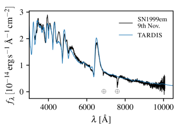
Figure 2: tardis spectral model (blue) for the observations of SN1999em (black) taken by Hamuy et al. (2001) on the 9th of November. We have smoothed the Monte Carlo spectrum using a Savitzky-Golay filter (Savitzky & Golay 1964). The observational data has been taken from the WISeREP archive (Yaron & Gal-Yam 2012) and has been de-reddened according to the Cardelli, Clayton, & Mathis (1989) law with a color excess of $E(B-V)=0.08$. To account for the peculiar velocity of the host galaxy, the observations have been blueshifted by $770\text{\,}\mathrm{km}\text{\,}{\mathrm{s}}^{-1}$ (see Leonard et al. 2002). Finally, the synthetic spectrum has been scaled to match the observed de-reddened flux $f_{\lambda}$. The main telluric features are marked with circled crosses.

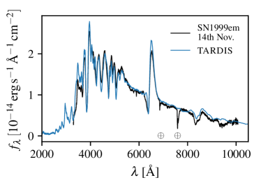
Figure 3: Same as footnote 1 but for the observations of SN1999em on the 14th of November.

5 Model grid

Having established the capabilities of the extended tardis version to produce accurate synthetic spectra for SNe II, we use the code to calculate an independent set of dilution factors. To this end, we have set up a grid of 343 models. These have been constructed to cover the interesting physical parameter space of inner boundary temperatures $T_{\mathrm{inner}}$ from $9500\text{\,}\mathrm{K}24\,000\text{\,}\mathrm{K}$, photospheric densities $\rho_{\mathrm{ph}}$ from $7\text{\times}{10}^{-15}\text{\,}\mathrm{g}\mathrm{/}\mathrm{c}\mathrm{m}\mathrm{{}^{3}}8\text{\times}{10}^{-14}\text{\,}\mathrm{g}\mathrm{/}\mathrm{c}\mathrm{m}\mathrm{{}^{3}}$, power-law density indexes $n$ from 6 to 14 and photospheric velocities $v_{\mathrm{ph}}$ from $3000\text{\,}\mathrm{km}\text{\,}{\mathrm{s}}^{-1}14\,000\text{\,}\mathrm{km}\text{\,}{\mathrm{s}}^{-1}$. For these parameters the models span a range of effective temperatures $T_{\mathrm{eff}}$ from $4900\text{\,}\mathrm{K}12\,000\text{\,}\mathrm{K}$. We take the photospheric properties $\rho_{\mathrm{ph}}$ and $v_{\mathrm{ph}}$ to refer to the position at which the electron scattering optical depth is $\tau=2/3$. In practice, the models are set up by adopting $\rho_{0}=\rho_{\mathrm{*}}$ and $r_{0}=v_{\mathrm{*}}t$ for the density profile (Eq. 23), where $\rho_{\mathrm{*}}$ and $v_{\mathrm{*}}$ are specific values selected from the desired range of photospheric density and velocity. To ensure that the photosphere of the model will lie at the appropriate depth, $t$ (time since explosion) is estimated using

$$t=\frac{2(n-1)m_{H}\mu_{e}}{3v_{\mathrm{*}}\rho_{\mathrm{*}}\sigma_{T}}$$ (35)

where $m_{H}$ is the mass of a hydrogen atom, $\mu_{\mathrm{e}}$ is the mean molecular weight per electron and $\sigma_{T}$ is the Thomson cross section. In making this estimate, it is assumed that $\mu_{e}$ is well-approximated by $\mu_{e}=1.52$, as appropriate for a composition of ionized hydrogen and singly-ionized helium. The full calculation is then carried out and the true values of $\rho_{\mathrm{ph}}$ and $v_{\mathrm{ph}}$ are extracted from the simulation. In general, the true values of the photospheric parameters ($\rho_{\mathrm{ph}}$, $v_{\mathrm{ph}}$) are very close to the originally selected reference parameters ($\rho_{\mathrm{*}}$, $v_{\mathrm{*}}$) from which the model was generated. Nevertheless, we always refer to each model by the derived (simulation) values of $\rho_{\mathrm{ph}}$ and $v_{\mathrm{ph}}$. We note that the true inner boundary of our computational domain lies considerably deeper than the (approximate) photosphere, typically at $\tau\sim 27$.

The setup of the model grid is done in the form of a latin hypercube design (Stein 1987). In this approach, each parameter range is subdivided into $N$ equal intervals, where $N$ is the number of models and one random parameter value is selected from each subinterval. This guarantees that, in contrast to a conventional cartesian grid, $N$ distinct values exist for each parameter. This is in particular beneficial if the quantities of interest are only weakly sensitive to a subset of parameters. Finally, to illustrate the properties of our set of models, a projection of the grid in the $T_{\mathrm{eff}}$ - $\rho_{\mathrm{ph}}$ plane is shown in Fig. 4. As can be seen, the desired parameter space is for the most part uniformly covered. Deviations from the uniform spacing arise from the use of Eq. 35 to map between photospheric quantities and the computational grid. This process becomes less reliable as soon as a strong recombination front develops. The main motivation for using a mostly uniform grid is that it allows us to study the differential influence of model parameters, such as the photospheric density, on the dilution factors. In this context, correlations between the input parameters have to be avoided as far as possible. However, since quantities such as photospheric temperature and density are certainly not completely independent in nature, this also means that the grid includes models that are not representative of normal SNe II. One example would be an object with a very high expansion velocity but an extremely low temperature.

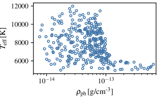
Figure 4: Illustration of the model grid from Sect. 5. The plot shows the effective temperature $T_{\mathrm{eff}}$ and the photospheric density $\rho_{\mathrm{ph}}$ for all atmosphere models. At low temperatures the actual photospheric density can exceed the targeted upper limit of $8\text{\times}{10}^{-14}\text{\,}\mathrm{g}\mathrm{/}\mathrm{c}\mathrm{m}\mathrm{{}^{3}}$, due the development of a strong recombination wave, which complicates the mapping between photospheric properties and the computational grid.

6 Results

6.1 Overview

From synthetic photometry of our model spectra, we can derive color temperatures $T_{S}$ and dilution factors $\xi_{S}$ according to Eq. 33. To facilitate the comparison to the results of E96 and D05, we focus our analysis on the bandpass combinations $S$={B,V}, {B,V,I}, {V,I} and {J,H,K} with filter functions taken from Bessell & Brett (1988) and Bessell (1990). Examples of the dilute blackbody models constructed in the synthetic EPM analysis are shown in Fig. 5.

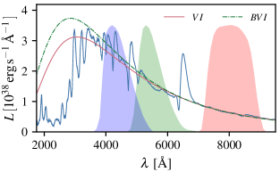
Figure 5: Comparison of the dilute blackbody models from {V,I} (red) and {B,V,I} synthetic photometry (green) to the original tardis spectrum (blue). The spectrum is our SN1999em model for the 9th of November (see footnote 1). The parameters of the blackbody fits are $T_{VI}=$9500\text{\,}\mathrm{K}$$, $T_{BVI}=$10\,200\text{\,}\mathrm{K}$$ and $\xi_{VI}=0.49$, $\xi_{BVI}=0.45$. We have overplotted the transmission curves for the B, V and I filters from Bessell (1990). The Monte Carlo spectrum has been smoothed using a Savitzky-Golay filter (Savitzky & Golay 1964).

The results of our analysis are summarized in Fig. 6, which displays dilution factors $\xi_{S}$ and color temperatures $T_{S}$ for all our models, as well as comparison values from E96 and D05. The color temperatures constitute the most important parameters in the study of the dilution factors, since they account for most of the variance in the correction factors and can be easily inferred from observations. Variations of the remaining parameters such as photospheric density or velocity are in most cases of secondary importance and are responsible for the observed dispersion around the color-temperature trend. In Fig. 6 we find good agreement with D05, in particular at low to medium color temperatures. For {B,V,I} and {V,I} the results match well for temperatures below $12\,500\text{\,}\mathrm{K}$ and for {J,H,K} for temperatures below $7000\text{\,}\mathrm{K}$. In {B,V} the dilution factors are similar to D05 over the entire temperature range. For higher color temperatures in {B,V,I}, {V,I}, and {J,H,K} our models tend to be systematically more dilute than D05 with values closer to those published by E96. As will be discussed in Sect. 7.2, part of this discrepancy can be attributed to differences in the adopted photospheric densities. We note that for all bandpass combinations the intrinsic scatter of our dilution factors is slightly larger than for the set of models by D05. This was to be expected, since we have constructed our grid of models in such a way that at all temperatures the whole range of remaining parameters is covered (see Sect. 5). In contrast, the dilution factors of E96 show a much smaller dispersion, since only a narrow part of the parameter space is explored in their study. Before concluding our discussion, we stress that this scatter does not correspond to the diversity of real objects but only reflects our ignorance about the parameter space occupied by SNe II. Finally, following E96 and D05 we present third order polynomial fits to the color temperature dependence of our dilution factors $\xi_{S}=\sum_{i}a_{i}(${10}^{4}\text{\,}\mathrm{K}$/T_{S})^{i}$ in Table 1.

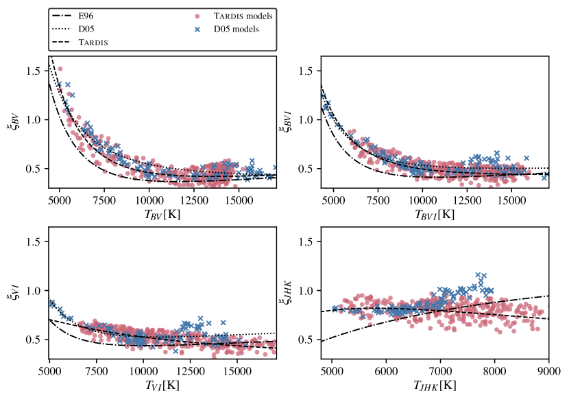
Figure 6: Dilution factors $\xi_{S}$ as a function of color temperature $T_{S}$ for filter combinations $S$={B,V}, {B,V,I}, {V,I} and {J,H,K}. We use a common y-axis scale for all bandpass combinations $S$ to highlight the differences in the scaling behavior of the dilution factors. For comparison purposes, we include the models of D05 as blue crosses. Polynomial fits to the dilution factors are shown for all sets of models (dashed: tardis, dashed dotted: E96, dotted: D05). For {J,H,K} the D05 curve is not included due to a misprint in the tabulated fit coefficients in the original paper.

	{B,V}	{B,V,I}	{V,I}	{J,H,K}
$a_{0}$	0.7417	0.5356	0.2116	-0.0384
$a_{1}$	-0.8662	-0.3355	0.3799	0.9918
$a_{2}$	0.5828	0.2959	-0.0673	-0.2867

Table 1: Coefficients $a_{i}$ of polynomial fits $\xi_{S}=\sum_{i}a_{i}(${10}^{4}\text{\,}\mathrm{K}$/T_{S})^{i}$ to the models for bandpass combinations $S$={B,V}, {B,V,I}, {V,I} and {J,H,K}.

.

6.2 Influence of atmospheric properties

In the previous section, the dependence of the dilution factors on temperature has been discussed. Here, we will focus on the effects of density. First, we analyze the variation of the dilution factors with photospheric density. Secondly, we investigate the influence of the steepness of the density profile. Finally, to conclude the discussion of the effect of model parameters, we will assess the robustness of the dilution factor fit curves against changes in the metallicity.

Influence of the photopsheric density

Variations in the photospheric density account for most of the dispersion of the models around the general color temperature dependence as illustrated in Fig. 7. Since the density cannot be easily constrained from observational data, it is essential to understand its influence on the dilution factors to quantify the associated uncertainties on the mean and the variance of the tabulated fit curves. Footnote 3 shows the density dependence of our dilution factors and a comparison to the results of D05. In general the dilution factors tend to increase with photospheric density, with the strength of the scaling varying between bandpass combinations. This behavior can be understood by remembering that the amount of continuum flux dilution depends on the ratio of continuum to scattering opacity (see Sect. 3.2). Since the main contribution to the scattering opacity comes from Thomson scattering, it is proportional to the electron density. Thermalization processes, on the other hand, roughly scale with the square of the electron density. As such, we expect the ratio of the two to increase with density, yielding a smaller amount of flux dilution at high densities. To study this behavior in a more quantitative way, we adopt the same ansatz as E96 for the dilution factors:

$$\xi_{S}=\rho_{\mathrm{ph}}^{\gamma}z(T_{S}).$$ (36)

Here, $z(T_{S})$ denotes a polynomial of the same form as those used in Table 1. A least squares fit to our set of models yields the density scaling indexes $\gamma$ listed in Table 2. Overall, the inferred density dependence of our dilution factors is moderate with similar magnitudes for all passbands. The scaling indexes $\gamma$ are systematically a bit larger than those published in E96 with the largest difference in the infrared (see Table 1). However, as illustrated by footnote 3 the density dependence in the infrared is not well described by a single power-law for the entire density range. In Sect. 7.2 we will use the inferred power-law scalings to assess whether differences in the assumed photospheric densities play an import role in understanding the discrepancies between the published sets of dilution factors.

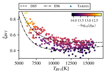
Figure 7: Dilution factors $\xi_{BVI}$ as a function of color temperature $T_{BVI}$. To illustrate the density dependence of our tardis models, the logarithm of the photospheric density $\log_{10}\rho_{\mathrm{ph}}$ is color-coded. For comparison purposes we include the polynomial fits to the dilution factors of E96 (dashed-dotted) and D05 (dashed).

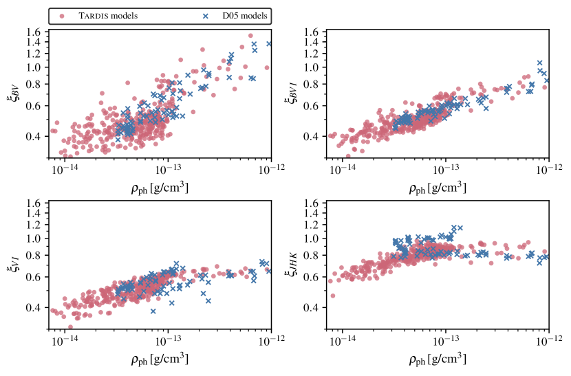
Figure 8: Variation of the dilution factors $\xi_{S}$ with photospheric density $\rho_{\mathrm{ph}}$ for filter combinations $S$={B,V}, {B,V,I}, {V,I} and {J,H,K}. For comparison purposes the models of D05 are shown as blue crosses.

	Models	{B,V}	{B,V,I}	{V,I}	{J,H,K}
$\gamma$	tardis E96	0.106 0.0776	0.137 0.0933	0.133 0.0769	0.116 0.0307

Table 2: Coefficients $\gamma$ of polynomial fits $\xi_{S}=\rho_{\mathrm{ph}}^{\gamma}z(T_{S})$ to the density dependence of the dilution factors for bandpass combinations $S$={B,V}, {B,V,I}, {V,I} and {J,H,K}. Here, $z(s)=\sum_{i}a_{i}(${10}^{4}\text{\,}\mathrm{K}$/T_{S})^{i}$ denotes a polynomial of the same form as used in Table 1 but with different fitted values for the coefficients.

Influence of the density structure

For a power-law atmosphere the ratio of photospheric density and density index $n$ is approximately given by

$$\frac{\rho_{\mathrm{ph}}}{n-1}\approx\frac{2}{3}\frac{\mu_{\mathrm{e}}}{\sigma_{\mathrm{e}}v_{\mathrm{ph}}t}\;\;.$$ (37)

For a given outflow ionization, time of explosion and expansion velocity, an increase in the density index $n$ results in higher photospheric densities $\rho_{\mathrm{ph}}$ and therefore less flux dilution. However, if the density structure is treated as an independent parameter, the dilution factors do not show a strong dependence on $n$ as illustrated by Fig. 9. For a possible explanation, we refer the reader to E96, who have found the same behavior and have proposed a physical motivation in their §3.3.

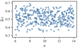
Figure 9: Dilution factors $\xi$ for the bandpass combination {V,I} as a function of the density indexes $n=-\mathop{}\!\mathrm{d}{\ln{\rho}}/\mathop{}\!\mathrm{d}{\ln{r}}$ of the power-law model atmospheres.

Influence of metallicity

Line blanketing by metals, in particular iron group elements, plays an important role in shaping the spectral energy distribution of SNe II and the resulting influence of metallicity on the emergent spectrum has been discussed in detail in the literature (see e.g., Dessart & Hillier 2005b). However, neither E96 nor D05 discuss in depth how this effect translates into changes in the dilution factors. To investigate the sensitivity of the $\xi$-$T$ fit curves to changes in metallicity, we have rerun a random subset of 68 models of our solar metallicity grid ($Z=1$) with a lower metallicity of $Z=0.2$. The resulting changes in the color temperatures and dilution factors are shown in Fig. 10 for the {B,V,I} bandpass combination. As expected, at high temperatures ($T_{BVI}\gtrapprox$10\,000\text{\,}\mathrm{K}$$) the influence of metallicity on the model properties is negligible, since the degree of ionization is too high for significant line blanketing to develop in the optical and near-UV. For moderate and low temperatures large changes in the color temperature up to thousands of degrees are observed. However, the associated changes in the dilution factors are approximately aligned with the general scaling of $\xi$ with $T$. Compared to the intrinsic scatter of the models, the induced changes in the functional behavior of $\xi$ with $T$ are of secondary importance. Thus, in the investigated regime, ranging from solar to distinctly subsolar, the tabulated fit curves are robust against modifications of the metallicity.

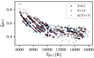
Figure 10: Change of dilution factors $\xi_{BVI}$ with metallicity $Z$. The subset of the original solar metallicty models for which corresponding calculations with a lower metallicity have been performed are shown in red. The metal-poor models are depicted in blue. Arrows illustrate the changes in model properties induced by the change to the subsolar metallicity of $Z=0.2$. To facilitate the comparison to the general $\xi$-$T$ trend, all models of the original grid are included in gray.

7 Comparison to previous studies

7.1 Radiative transfer

To put our results into context, we review differences in the radiative transfer modeling between the Cmfgen code used by D05, the Eddington code used by E96 and tardis and discuss possible effects on the dilution factors. The main differences lie in the ionization treatment of metal species, the handling of line opacity and the inclusion of relativistic transfer effects.

For the calculations presented by D05, only the effect of the Doppler shift on the frequency of the radiation field is taken into account. E96 follow a different approach based on the premise that radiation-field time dependence can be included in a quasi-static treatment by enforcing a constant luminosity in the comoving frame. In this case, the time-dependent comoving-frame transport equation reduces to a much simpler expression that differs from D05 only by an additional term $\beta I_{\nu}/r$, where $I_{\nu}$ is the specific intensity of the radiation field. This term is formally identical to the part of the full transport equation that describes the redshift of photons in the scattering process and thus the adiabatic loss of radiation energy. However, the sign is changed and the magnitude decreased by a factor of three. Both approaches neglect the so-called advection term that arises from the frame transformation of angles (see e.g., Pistinner & Shaviv 1994, for a discussion). This term is generally deemed to be more important than the aberration term (see e.g., Baron et al. 1996b). Taking into account the additional reduction of the magnitude of the aberration term in E96, we conclude that the differences in handling the relativistic terms between E96 and D05 are small in comparison to our relativistic treatment (Sect. 2.1.4), which corresponds to a full solution of the quasi-static relativistic transport problem. Since we can achieve good agreement with D05 despite this difference, we consider it unlikely that relativistic effects play an important role in explaining the systematic offset between E96 and D05.

Another possible source for discrepancies, which has been discussed previously in the literature (see D05, ), is the treatment of line interactions. Here, the differences start with the handling of the opacity. Both Cmfgen (D05) and tardis treat the contributions of all lines to the opacity individually, in a consistent manner. In contrast, Eddington (E96) adopts the more convenient but approximate expansion opacity formalism of Eastman & Pinto (1993) that combines all line opacity in a wavelength bin. For the opacity calculation, the expansion opacity formalism in E96, as well as the method used in tardis, rely on the Sobolev approximation (Sobolev 1957), whereas Cmfgen adopts the comoving-frame method. For micro-turbulent velocities of less than $100\text{\,}\mathrm{km}\text{\,}{\mathrm{s}}^{-1}$, as adopted in D05, the Sobolev method is of similar accuracy as the comoving-frame method in describing the formation of hydrogen lines in SNe II (see Duschinger et al. 1995). In regions where line overlap is possible, in particular in the metal line forest in the blue, the Sobolev approximation may, however, be less accurate than the comoving-frame method.

With respect to line interactions, the final difference between the codes concerns the redistribution of the absorbed radiation. Only Cmfgen computes a full NLTE source function for all included species. In E96 line interactions are treated in detail only for a few selected elements, in most cases only hydrogen. For the remaining species, resonance scattering is assumed and effects such as fluorescence or collisional deexcitations are neglected. tardis strikes a balance between the approximate treatment of E96 and the full NLTE calculation of D05. In principle, our implementation of the macro atom scheme of Lucy (2002, 2003) also provides a full NLTE description of the redistribution process. However, in our simulations only radiative and collisional bound-bound transitions are included for species other than hydrogen. Despite this simplification, the approximate NLTE emissivities from the macro atom provide a full treatment of fluorescence. It is also worth pointing out that the predicted emissivities are largely insensitive to errors in the excited states population and therefore to our use of approximate excitation treatments. This has been demonstrated by Lucy (2002) and may be understood by considering that, in the context of the macro atom machinery, the most relevant level number densities are those of the ground state and low-lying metastable levels. Radiative excitations from these states account for most of the activations of the macro atom and their populations are likely to be close to LTE with respect to the ground state. In contrast, the level number densities of excited states, which will be less accurately estimated, are not as important in setting the rate of macro atom activations and enter in the emissivity only through minor modifications of the internal redistribution probabilities for stimulated emission. Thus we argue that the macro atom approach captures most of the essential physics of a full NLTE treatment as opposed to the resonance scattering approximation used in E96. As such, it constitutes a promising source of systematic discrepancies between E96 on the one hand and D05 and tardis on the other hand.

To conclude our discussion of the major differences in the numerical treatments, we compare the different methods used for calculating the ionization state of metal species. An accurate solution to the ionization balance is essential in modeling the line blanketing, which shapes the spectral energy distribution in the blue. Due to the use of super-levels, Cmfgen (D05) is able to consistently, though approximately, treat all species in NLTE. In contrast, E96 calculated the ionization using NLTE only for a few selected species and only for a subset of their atmospheric models. For the remaining models and species, LTE at the electron temperature is assumed. Similarly, tardis relies on simplified prescriptions for the calculation of the ionization balance of metals. For the results presented in this paper, we have used the nebular ionization approximation of Mazzali & Lucy (1993). In principle, this method should provide a more accurate description of the ionization balance in a diluted, radiation- dominated environment than the assumption of LTE. However, neither assumption can fully replace a detailed photoionization calculation. Still, our spectral models for SN1999em (see Sect. 4) reproduce the observed line blanketing well. This instills confidence that, at least for the early and intermediate stage evolution, the nebular ionization treatment adequately captures the essential physics.

Ultimately, it is extremely difficult to assess the extent to which, if at all, individual numerical differences contribute to the systematic discrepancy between the sets of dilution factors. Based on qualitative arguments, we have deemed it unlikely that the handling of relativistic terms plays an important role in this context. We have identified the use of the very simple resonance scattering approximation by E96 as one of the main distinguishing features from both our and D05’s numerical approaches. As such, it can be regarded as a promising possible contributory factor to the systematic differences. However, these interpretations are speculative and should be taken with a grain of salt.

7.2 Effect of model grid assumptions

In the previous section we have discussed how differences in the radiative transfer calculations can affect the dilution factors. In the context of the discrepancy between E96 and D05 most of the discussion in the literature (see e.g., Dessart & Hillier 2005a; Jones et al. 2009) has revolved around these issues. However, another possibly important (albeit banal) source of systematic differences is the choice of model grid properties. To demonstrate this, we have modified the plot depicting the temperature dependence of our dilution factors for the {B,V,I} bandpass combination to include the color-coded photospheric density for each model (see Fig. 7). From this, it is obvious that the inferred fit curves can easily be moved upwards or downwards by preferentially sampling either the high density or the low density regions of the parameter space. Since the exact distribution and correlation of parameters such as density, temperature and velocity are not known for the population of SNe II, there exists a certain amount of freedom in the setup of the model grid.

To quantitatively illustrate the role such effects may have, we have investigated the influence of density in particular. For a comparative study we need to consider families of models for which color temperature, densities and dilution factors are available – accordingly, we make use of our tardis models, the E96 models and the models presented for the tailored EPM analysis of SN1999em, SN2005s and SN2006bp (Dessart & Hillier 2006; Dessart et al. 2008). This set of 38 models covers the relevant range of color temperatures and generally follows the fit curves published in D05.

Before we compare densities, we approximately correct for changes of the electron densities between the set of models due to differences in composition (specifically, we rescale the densities from E96’s models with the estimated ratio of the mean molecular weights per electron). The mean rescaled densities $\langle\rho_{\mathrm{ph}}\rangle$ are shown in Fig. 11 as a function of {B,V,I} color temperature. Overall, the densities used in this paper, and in Dessart & Hillier (2006) and Dessart et al. (2008) tend to be larger than those of E96 with maximum differences of a factor of a few. The conspicuous jump in density for the E96 models between 8000 and 9000 K stems from two exponential atmospheres (e12.2,e12.3). To check whether this density mismatch might alleviate some of the tension between the dilution factors by E96, and those of Dessart & Hillier (2005a, 2006) and Dessart et al. (2008), we rescale the dilution factors $\xi_{\mathrm{S}}$ using the simple power-law relation $\xi_{S}\propto\rho_{\mathrm{ph}}^{\gamma}$ from Sect. 6.2. For this purpose we do not use the mean densities $\langle\rho_{\mathrm{ph}}\rangle$ from Fig. 12 but the appropriate average $\langle\rho_{\mathrm{ph}}^{\gamma}\rangle^{1/\gamma}$. Fig. 12(a) illustrates the effect of the rescaling on the discrepancy between the two sets of models. Applying the density correction reduces the maximum difference from roughly 40% to 20%, but fails to remove the systematic offset completely. As can be seen in Fig. 12(b), the procedure is more successful for our set of dilution factors. After rescaling, only a maximum difference of around 8% remains between our calculations and those of Dessart & Hillier (2006) and Dessart et al. (2008). We stress that due to the simplifying assumptions we have made the results above are only qualitative in nature. Nevertheless, our discussion demonstrates that differences in the setup of the model grid, for example different choices for the photospheric densities, can introduce systematic uncertainties on the 10% level in the dilution factors. This most likely explains part of the discrepancy between the results of E96, and those of Dessart & Hillier (2005a, 2006) and Dessart et al. (2008). To eliminate this additional error source, approaches are needed that strongly constrain the relevant parameters through observational data. One possibility would be to base the dilution factor fit curves on the tailored EPM analyses of a representative set of SNe IIP.

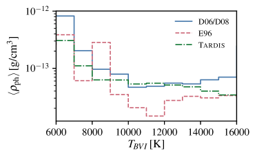
Figure 11: Comparison of the mean photospheric density $\langle\rho_{\mathrm{ph}}\rangle$ at a given {B,V,I} color temperature for the models from E96 (red dashed), the tailored EPM analyses of Dessart & Hillier (2006) and Dessart et al. (2008) (D06/D08, blue solid), and this paper (green dash-dotted). The plotted densities have been rescaled slightly to account for differences in the composition as outlined in Sect. 7.2.

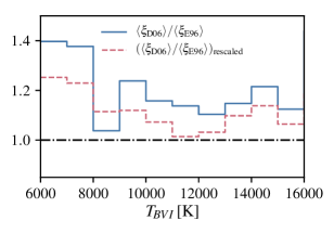
(a)

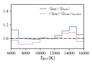
(b)

Figure 12: Comparison of the discrepancy between the dilution factor set in the {B,V,I} bandpass combination of Dessart & Hillier (2006) and Dessart et al. (2008) $\langle\xi_{\mathrm{D06}}\rangle$, and E96 $\langle\xi_{\mathrm{E96}}\rangle$ (upper panel, a), and with respect to the results of this paper $\langle\xi_{\mathrm{Tardis}}\rangle$ (lower panel, b). The findings before (blue solid) and after (red dashed) the application of a density correction factor are shown. The details of the procedure are described in Sect. 7.2.

8 Conclusions

In this work, we present an extension of the Monte Carlo radiative transfer code tardis to the spectral synthesis of SNe IIP. The key feature of our numerical approach is an updated radiation–matter interaction scheme, which provides a full treatment of bound-bound, bound-free, free-free and collisional processes based on the macro atom scheme of Lucy (2002, 2003). The second major improvement concerns the calculation of the plasma state. The code now contains a self-consistent determination of the thermal structure from the heating and cooling balance as well as a full NLTE calculation of the ionization and excitation state for hydrogen. Other changes include an improved handling of relativistic effects, an adaption of the spectral synthesis calculation for high optical depths and a different initialization of the plasma state. We demonstrate the capabilities of the extended code by modeling two different epochs of the prototypical SN II SN1999em. For both epochs good agreement with the observed spectra is achieved, instilling confidence that tardis is well-suited for quantitative spectroscopic analysis of photospheric-phase, hydrogen-rich supernovae.

In line with our goal to use tardis for measuring distances, our final application is the calculation of an independent set of EPM dilution factors. In this context, a long-standing issue has been the systematic discrepancy of around 20% between the results of E96 and D05, which translates into an uncertainty of the EPM distance of the same magnitude. To address this problem, we have performed radiative transfer calculations for a set of 343 tardis models, which span a wide range of temperatures, densities and expansion velocities. Despite using significantly different numerical techniques, the dilution factors extracted from these calculations show good agreement with those published by D05. This result helps remove some of the tension between the available sets of distance correction factors. It is still somewhat unclear which differences in the numerical approach make the models of E96 systematically more dilute than ours and D05’s. Based on our calculations, we can plausibly rule out only one of the previously suggested explanations, namely differences in the treatment of relativistic effects.

Our other focus lay on investigating the parameter dependences of the dilution factors. Similar to E96 and D05, we identify density as one of the most important parameters in setting the magnitudes of the dilution factors. Our power-law fits to the density dependence yield similar scaling behaviors as for the calculations by E96. As in E96, we do not find a strong effect of the steepness of the density profile. In addition, we have demonstrated that changing the metallicity from solar to decidedly subsolar (Z=0.2) only induces minor modifications in the relationship between color temperature and dilution factors.

Finally, we have investigated differences in the setup of the model grid as an additional source of systematic errors. In our discussion, we have demonstrated that part of the discrepancy between E96 and D05 can plausibly be tracked back to differences in the assumed photospheric densities. This result highlights the need to base tabulated dilution factors on approaches that constrain the model parameters and their correlations more strongly through observational data. One way to achieve this would be to apply the tailored EPM technique (Dessart & Hillier 2006; Dessart et al. 2008) to a representative set of SNe II.

In this paper we have established tardis as a new independent numerical tool for modeling SNe IIP and have demonstrated its capability to calculate accurate dilution factors. As a next step we plan to apply the code to measure absolute distances using the tailored EPM method (Dessart & Hillier 2006; Dessart et al. 2008) or SEAM (Baron et al. 1995, 1996a, 2004, 2007). As a consequence of the inclusion of a much more detailed treatment of the radiative transfer process, the typical runtime of the tardis spectral synthesis procedure has increased from minutes needed in the original implementation by Kerzendorf & Sim (2014) to hours. However, in light of the ubiquity of machine learning techniques and the continuous increase in computational resources, this increase in computational complexity is of minor concern and it will, for the first time, be feasible to perform the spectral fitting process in an automated manner. In combination with sampling techniques the parameter space can be explored in a systematic manner and uncertainties in the estimated parameters can be obtained. This will put strong constraints on the accuracy of absolute distance measurements of SNe II and will help to assess their promise as tools for cosmology.