Regret Circuits: Composability of Regret Minimizers

Abstract

Regret minimization is a powerful tool for solving large-scale problems; it was recently used in breakthrough results for large-scale extensive-form game solving. This was achieved by composing simplex regret minimizers into an overall regret-minimization framework for extensive-form game strategy spaces. In this paper we study the general composability of regret minimizers. We derive a calculus for constructing regret minimizers for composite convex sets that are obtained from convexity-preserving operations on simpler convex sets. We show that local regret minimizers for the simpler sets can be combined with additional regret minimizers into an aggregate regret minimizer for the composite set. As one application, we show that the CFR framework can be constructed easily from our framework. We also show ways to include curtailing (constraining) operations into our framework. For one, they enables the construction of CFR generalization for extensive-form games with general convex strategy constraints that can cut across decision points.

1 Introduction

Counterfactual regret minimization (CFR) (Zinkevich et al., 2007), and its newer variants (Lanctot et al., 2009; Brown & Sandholm, 2015a; Tammelin et al., 2015; Brown et al., 2017; Brown & Sandholm, 2017a; 2019), have been a central component in several recent milestones in solving imperfect-information extensive-form games (EFGs). Bowling et al. (2015) used CFR⁺ to near-optimally solve heads-up limit Texas hold’em. Brown & Sandholm (2017c) used CFR variants, along with other scalability techniques such as real-time endgame solving (Ganzfried & Sandholm, 2015; Burch et al., 2014; Moravcik et al., 2016; Brown & Sandholm, 2017b) and automated action abstraction Brown & Sandholm (2014), to create Libratus, an AI that beat top human specialist professionals at the larger game of heads-up no-limit Texas hold’em. Moravčík et al. (2017) also used CFR variants and endgame solving to beat professional human players at that game.

CFR and its newer variants are usually presented as algorithms for finding an approximate Nash equilibrium in zero-sum EFGs. However, an alternative view is that it is a framework for constructing regret minimizers for the types of action spaces encountered in EFGs, as well as single-agent sequential decision making problems with similarly-structured actions spaces. Viewed from a convex optimization perspective, the class of convex sets to which they apply are sometimes referred to as treeplexes (Hoda et al., 2010; Kroer et al., 2015; 2018). In this view, those algorithms specify how a set of regret minimization algorithms for simplexes and linear loss functions can be composed to form a regret minimizer for a treeplex. Farina et al. (2019) take this view further, describing how regret-minimization algorithms can be composed to form regret minimizers for a generalization of treeplexes that allows convex sets and convex losses. This decomposition into individual optimization problems can be beneficial because it enables the use of 1) different algorithms for different parts of the search space, 2) specialized techniques for different parts of the problem, such as warm starting (Brown & Sandholm, 2014; 2015b; 2016) and pruning (Lanctot et al., 2009; Brown & Sandholm, 2015a; Brown et al., 2017; Brown & Sandholm, 2017a), and 3) approximation of some parts of the space.

In this paper we introduce a general methodology for composing regret minimizers. We derive a set of rules for how regret minimizers can be constructed for composite convex sets via a calculus of regret minimization: given regret minimizers for convex sets ${\cal X},{\cal Y}$ we show how to compose these regret minimizers for various convexity-preserving operations performed on the sets (e.g., intersection, convex hull, Cartesian product), in order to arrive at a regret minimizer for the resulting composite set.

Our approach treats the regret minimizers for individual convex sets as black boxes, and builds a regret minimizer for the resulting composite set by combining the outputs of the individual regret minimizers. This is important because it allows freedom in choosing the best regret minimizer for each individual set (from either a practical or theoretical perspective). For example, in practice the regret matching (Hart & Mas-Colell, 2000) and regret matching⁺ (RM⁺) (Tammelin et al., 2015) regret minimizers are known to perform better than theoretically-superior regret minimizers such as Hedge (Brown et al., 2017), while Hedge may give better theoretical results when trying to prove the convergence rate of a construction through our calculus.

One way to conceptually view our construction is as regret circuits: in order to construct a regret minimizer for some convex set ${\cal X}$ that consists of convexity-preserving operations on (say) two sets ${\cal X}_{1},{\cal X}_{2}$, we construct a regret circuit consisting of regret minimizers for ${\cal X}_{1}$ and ${\cal X}_{2}$, along with a sequence of operations that aggregate the results of those circuits in order to form an overall circuit for ${\cal X}$. We use this view extensively in the paper; we show the regret-circuit representation of every operation that we develop.

As an application, we show that the correctness and convergence rate of the CFR algorithm can be proven easily through our calculus. We also show that the recent Constrained CFR algorithm (Davis et al., 2019) can be constructed via our framework. Our framework enables the construction of two algorithms for that problem. The first is based on Lagrangian relaxation, and only guarantees approximate feasibility of the output strategies. The second is based on projection and guarantees exact feasibility, for the first time in any algorithm that decomposes overall regret into local regrets at decision points.

2 Regret Minimization

We will prove our results in the online learning framework called online convex optimization (Zinkevich, 2003) (OCO). In OCO, a decision maker repeatedly interacts with an unknown environment by making a sequence of decisions $x^{1}$, $x^{2},\dots$ from a convex and compact set ${\cal X}\subseteq\mathbb{R}^{n}$. After each decision $x^{t}$, the decision maker faces a convex loss function $\ell^{t}(x^{t})$, which is unknown to the decision maker until after the decision is made. So, we are constructing a device that supports two operations: (i) it provides the next decision $x^{t+1}\!\in\!{\cal X}$ and (ii) it receives/observes the convex loss function $\ell^{t}$ used to “evaluate” decision $x^{t}$. The decision making is online in the sense that the next decision, $x^{t+1}$, is based only on the previous decisions $x^{1},\dots,x^{t}$ and corresponding observed loss functions $\ell^{1},\dots,\ell^{t}$.

The quality of the device is measured by its cumulative regret, which is the difference between the loss cumulated by the sequence of decisions $x^{1},\dots,x^{T}$ and the loss that would have been cumulated by playing the best-in-hindsight time-independent decision $\hat{x}$. Formally, the cumulative regret up to time $T$ is

$$R_{({\cal X},{\cal F})}^{T}\mathrel{:\mkern-0.25mu=}\sum_{t=1}^{T}\ell^{t}(x^{t})-\min_{\hat{x}\in{\cal X}}\left\{\sum_{t=1}^{T}\ell^{t}(\hat{x})\right\}\!.$$ (1)

Above we introduce the new notation of a subscript $({\cal X},{\cal F})$ to be explicit about the domain of the decisions $\{x^{t}\}$ and the domain of the loss functions $\{\ell^{t}\}$, respectively. This turns out to be important because we will study composability of devices with different domains.

The device is called a regret minimizer if it satisfies the desirable property of Hannan consistency: the average regret approaches zero, that is, $R_{({\cal X},{\cal F})}^{T}$ grows sublinearly in $T$. Formally, in our notation, we have the following definition.

Definition 1 ($({\cal X},{\cal F})$-regret minimizer).

Let ${\cal X}$ be a convex and compact set, and let ${\cal F}$ be a convex cone in the space of bounded convex functions on ${\cal X}$, and such that ${\cal F}$ contains the space $\mathcal{L}$ of linear functions. An $({\cal X},{\cal F})$-regret minimizer is a function that selects the next decision $x^{t+1}\in{\cal X}$ given the history of decisions $x^{1},\dots,x^{t}$ and observed loss functions $\ell^{1},\dots,\ell^{t}\in{\cal F}$, so that the cumulative regret $R_{({\cal X},{\cal F})}^{T}=o(T)$.

2.1 Universality of Linear Loss Functions

Regret minimizers for linear loss functions are in a sense universal: one can construct a regret minimizer for convex loss functions from any regret minimizer for linear loss functions (e.g., McMahan (2011)). The crucial insight is that the regret that we are trying to minimize, $R_{({\cal X},{\cal F})}^{T}$, is bounded by the regret of a $({\cal X},{\cal L})$-regret minimizer that, at each time $t$, observes as its loss function a tangent plane of $\ell^{t}$ at the most recent decision $x^{t}$. Thus we can minimize $R_{({\cal X},{\cal F})}^{T}$ by minimizing $R^{T}_{({\cal X},{\cal L})}$.

Formally, let $\partial\ell^{t}(x^{t})$ be any subgradient of $\ell^{t}$ at $x^{t}$. By convexity of $\ell^{t}$,

$$\ell^{t}(\hat{x})\geq\ell^{t}(x^{t})+\langle\partial\ell^{t}(x^{t}),\,\hat{x}-x^{t}\rangle\quad\forall\,\hat{x}\in{\cal X},$$

and, substituting into (1), we obtain

$$R_{({\cal X},{\cal F})}^{T} \leq\sum_{t=1}^{T}\langle\partial\ell^{t}(x^{t}),\,x^{t}\rangle-\min_{{\hat{x}}\in\mathcal{X}}\left\{\sum_{t=1}^{T}\langle\partial\ell^{t}(x^{t}),\,\hat{x}\rangle\!\right\}\!,$$ (2)

where the right hand side is $R^{T}_{({\cal X},{\cal L})}$, the regret cumulated by a device that observes the linear loss functions $\langle\partial\ell^{t}(x^{t}),\cdot\,\rangle$.

2.2 Connection to Convex-Concave Saddle-Point Problems and Game Theory

In this subsection we review how regret minimization can be used to compute solutions to regularized bilinear saddle-point problems, that is solutions to problems of the form

$$\min_{x\in{\cal X}}\max_{y\in{\cal Y}}\big{\{}x^{\!\top}\!Ay+d_{1}(x)-d_{2}(y)\big{\}},$$ (3)

where ${\cal X},{\cal Y}$ are closed convex sets, and $d_{1},d_{2}$ are convex functions. This general formulation allows us to capture, among other settings, several game-theoretical applications such as computing Nash equilibria in two-player zero-sum games. In that setting, $d_{1}$ and $d_{2}$ are the constant zero functions, ${\cal X}$ and ${\cal Y}$ are convex polytopes whose description is provided by the sequence-form constraints, and $A$ is a real payoff matrix (von Stengel, 1996).

In order to use regret minimization to solve problems of the form (3), we consider the loss functions

$$\ell^{t}_{\cal X}:{\cal X}\ni x \mapsto(-Ay^{t})^{\!\top}x+d_{1}(x),$$

$$\ell^{t}_{\cal Y}:{\cal Y}\ni y \mapsto(A^{\top}x^{t})^{\!\top}y+d_{2}(y).$$

The error metric that we use is the saddle-point residual (or gap) $\xi$ of $(\bar{x},\bar{y})$, defined as

$$\max_{\hat{y}\in{\cal Y}}\{d_{1}\!(\bar{x})\!-\!d_{2}(\hat{y})\!+\!\langle\bar{x},A\hat{y}\rangle\!\}\!-\!\min_{\hat{x}\in{\cal X}}\{d_{1}\!(\hat{x})\!-\!d_{2}(\bar{y})\!+\!\langle\hat{x},A\bar{y}\rangle\!\}.$$

The following folk theorem shows that the average of a sequence of regret-minimizing strategies for the choice of losses above leads to a bounded saddle-point residual (see, for example, Farina et al. (2019) for a proof).

Theorem 1.

If the average regret accumulated on ${\cal X}$ and ${\cal Y}$ by the two sets of strategies $\{x_{t}\}_{t=1}^{T}$ and $\{y_{t}\}_{t=1}^{T}$ is $\epsilon_{1}$ and $\epsilon_{2}$, respectively, then the strategy profile $(\bar{x},\bar{y})$ where $\bar{x}=\frac{1}{T}\sum_{t=1}^{T}x^{t},\ \bar{y}=\frac{1}{T}\sum_{t=1}^{T}y^{t}$ has a saddle-point residual bounded above by $\epsilon_{1}+\epsilon_{2}$.

When $d_{1}\equiv d_{2}\equiv 0$ and ${\cal X},{\cal Y}$ are the players’ sequence-form strategy spaces, Theorem 1 asserts that the average strategy profile produced by the regret minimizers is an $(\epsilon_{1}+\epsilon_{2})$-Nash equilibrium.

Different choices of the regularizing functions $d_{1}$ and $d_{2}$ can be used to solve for strategies in other game-theoretic applications as well, such as computing a normal-form quantal-response equilibrium (Ling et al., 2018; Farina et al., 2019), and several types of opponent exploitation. Farina et al. (2019) study opponent exploitation where the goal is to compute a best response, subject to a penalty for moving away from a precomputed Nash equilibrium strategy; this is captured by having $d_{1}$ or $d_{2}$ include a penalty term that penalizes distance from the Nash equilibrium strategy. Farina et al. (2017) and Kroer et al. (2017) study constraints on individual decision points, and Davis et al. (2019) study additional constraints on the overall EFG polytopes ${\cal X},{\cal Y}$. Regret minimization in those settings requires regret minimizers that can operate on more general domains ${\cal X},{\cal Y}$ than the sequence form. In this paper we show how one can construct regret minimizers for any convex domain that can be constructed inductively from simpler domains using convexity-preserving operations.

3 Regret Circuits

In this paper, we introduce regret circuits. They are composed of independent regret minimizers connected by wires on which the loss functions and decisions can flow. Regret circuits encode how the inputs and outputs of multiple regret minimizers can be combined to achieve a goal, in a divide-and-conquer fashion, and help simplify the design and analysis of regret-minimizing algorithms. Using the constructions that we will present, one can compose different regret circuits and produce increasingly complex circuits.

The regret circuits approach has several advantages that make it appealing when compared to other, more monolithic, approaches. For one, by treating every regret minimizer that appears in a regret circuit as an independent black box, our approach enables one to select the best individual algorithm for each of them. Second, our framework is amenable to pruning or warm-starting techniques in different parts of the circuit, and substituting one or more parts of the circuit with an approximation. Finally, regret circuits can be easily run in distributed and parallel environments.

We will express regret circuits pictorially through block diagrams. We will use the following conventions when drawing regret circuits:

• an $({\cal X},{\cal F})$-regret minimizer is drawn as a box

  where the input (red) arrow represents the loss at a generic time $t-1$, while the output (blue) arrow represents the decision produced at time $t$;

• the symbol is used to denote an operation that constructs or manipulates one or more loss functions;

• the symbol is used to denote an operation that combines or manipulates one or more decisions;

• the symbol denotes an adder, that is a node that outputs the sum of all its inputs;

• dashed arrows denote decisions that originate from the previous iteration.

As an example, consider the construction of Section 2.1, where we showed how one can construct a regret minimizer for generic convex loss functions from any regret minimizer for linear loss functions. Figure 1 shows how that construction can be expressed as a regret circuit.

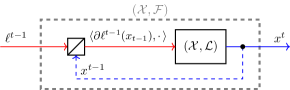
Figure 1: Regret circuit representing the construction of an $({\cal X},{\cal F})$-regret minimizer using an $({\cal X},{\cal L})$-regret minimizer.

4 Circuit Construction for Operations that Enlarge or Transform Sets

In this section, we begin the construction of our calculus of regret minimization. Given regret minimizers for two closed convex sets ${\cal X}$ and ${\cal Y}$, we show how to construct a regret minimization for sets obtained via convexity-preserving operations on ${\cal X}$ and ${\cal Y}$. In this section, we focus on operations that take one or more sets and produce a regret minimizer for a larger set—this is the case, for instance, of convex hulls, Cartesian products, and Minkowski sums.

As explained in Section 2.1, one can extend any $({\cal X},{\cal L})$-regret minimizer to handle more expressive loss functionals. Therefore, in the rest of the paper, we focus on $({\cal X},{\cal L})$-regret minimizers.

4.1 Cartesian Product

In this section, we show how to combine an $({\cal X},{\cal L})$- and a $({\cal Y},{\cal L})$-regret minimizer to form an $({\cal X}\times{\cal Y},{\cal L})$-regret minimizer. Any linear function $\ell:{\cal X}\times{\cal Y}\to\mathbb{R}$ can be written as $\ell(x,y)=\ell_{\cal X}(x)+\ell_{\cal Y}(y)$ where the linear functions $\ell_{\cal X}:{\cal X}\to\mathbb{R}$ and $\ell_{\cal Y}:{\cal Y}\to\mathbb{R}$ are defined as $\ell_{\cal X}:x\mapsto\ell(x,0)$ and $\ell_{\cal Y}:y\mapsto\ell(0,y)$. It is immediate to verify that

$$R^{T}_{({\cal X}\times{\cal Y},{\cal L})} =\left(\sum_{t=1}^{T}\ell_{\cal X}^{t}(x^{t})-\min_{\hat{x}\in{\cal X}}\left\{\sum_{t=1}^{T}\ell_{\cal X}^{t}(\hat{x})\right\}\right)$$

$$\hskip 28.45274pt+\left(\sum_{t=1}^{T}\ell_{\cal Y}^{t}(y^{t})-\min_{\hat{y}\in{\cal Y}}\left\{\sum_{t=1}^{T}\ell_{\cal Y}^{t}(\hat{y})\right\}\right)$$

$$=R^{T}_{({\cal X},{\cal L})}+R^{T}_{({\cal Y},{\cal L})}.$$

In other words, it is possible to minimize regret on ${\cal X}\times{\cal Y}$ by simply minimizing it on ${\cal X}$ and ${\cal Y}$ independently and then combining the decisions, as in Figure 2.

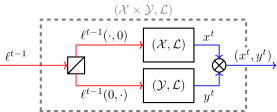
Figure 2: Regret circuit for the Cartesian product ${\cal X}\times{\cal Y}$.

4.2 Affine Transformation and Minkowski Sum

Let $T:E\to F$ be an affine map between two Euclidean spaces $E$ and $F$, and let ${\cal X}\subseteq E$ be a convex and compact set. We now show how an $({\cal X},{\cal L})$-regret minimizer can be employed to construct a $(T({\cal X}),{\cal L})$-regret minimizer.

Since every $y\in T({\cal X})$ can be written as $y=T(x)$ for some $x\in{\cal X}$, the cumulative regret for a $(T({\cal X}),{\cal L})$-regret minimizer can be expressed as

$$R_{(T({\cal X}),{\cal L})}^{T} =\sum_{t=1}^{T}(\ell^{t}\circ T)(x^{t})-\min_{\hat{x}\in{\cal X}}\left\{\sum_{t=1}^{T}(\ell^{t}\circ T)(\hat{x})\right\}\!.$$

Since $\ell^{t}$ and $T$ are affine, their composition $\ell_{T}^{t}\mathrel{:\mkern-0.25mu=}\ell^{t}\circ T$ is also affine. Hence, $R_{(T({\cal X}),{\cal L})}^{T}$ is the same regret as an $({\cal X},{\cal L})$-regret minimizer that observes the linear function $\ell_{T}^{t}(\cdot)-\ell_{T}^{t}(0)$ instead of $\ell^{t}$.The construction is summarized by the circuit in Figure 3.

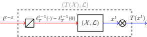
Figure 3: Regret circuit for the image $T({\cal X})$ of ${\cal X}$ under the affine transformation $T$.

As an application, we use the above construction to form a regret minimizer for the Minkowski sum ${\cal X}+{\cal Y}:=\{x+y:x\in{\cal X},y\in{\cal Y}\}$ of two sets. Indeed, note that ${\cal X}+{\cal Y}=\sigma({\cal X}\times{\cal Y})$, where $\sigma:(x,y)\mapsto x+y$ is a linear map. Hence, we can combine the construction in this section together with the construction of the Cartesian product (Figure 2). See Figure 4 for the resulting circuit.

Figure 4: Regret circuit for the Minkowski sum ${\cal X}+{\cal Y}$ (Section 4.2).

4.3 Convex Hull

In this section, we show how to combine an $({\cal X},{\cal L})$- and a $({\cal Y},{\cal L})$-regret minimizer to form a $(\mathop{{\rm co}}\{{\cal X},{\cal Y}\},{\cal L})$-regret minimizer, where $\mathop{{\rm co}}$ denotes the convex hull operation,

$$\mathop{{\rm co}}\{{\cal X},{\cal Y}\}=\{\lambda_{1}x+\lambda_{2}y\ :\ x\in{\cal X},y\in{\cal Y},(\lambda_{1},\lambda_{2})\in\Delta^{2}\},$$

and $\Delta^{2}$ is the two-dimensional simplex

$$\Delta^{2}\mathrel{:\mkern-0.25mu=}\{(\lambda_{1},\lambda_{2})\in\mathbb{R}^{2}_{+}:\lambda_{1}+\lambda_{2}=1\}.$$

Hence, we can think of a $(\mathop{{\rm co}}\{{\cal X},{\cal Y}\},{\cal L})$-regret minimizer as picking a triple $(\lambda^{t},x^{t},y^{t})\in\Delta^{2}\times{\cal X}\times{\cal Y}$ at each time point $t$. Using the linearity of the loss functions,

$$R^{T}_{(\mathop{{\rm co}}\{{\cal X},{\cal Y}\},{\cal L})} =\left(\sum_{t=1}^{T}\lambda_{1}^{t}\ell^{t}(x^{t})+\lambda_{2}^{t}\ell^{t}(y^{t})\right)$$

$$\hskip 17.07182pt-\!\!\!\min_{\begin{subarray}{c}\hat{\lambda}\in\Delta^{2}\\ \hat{x}\in{\cal X},\hat{y}\in{\cal Y}\end{subarray}}\!\left\{{\hat{\lambda}_{1}}\sum_{t=1}^{T}\ell^{t}(\hat{x})+\hat{\lambda}_{2}\sum_{t=1}^{T}\ell^{t}(\hat{y})\right\}\!.$$

Now, we make two crucial observations. First,

$$\min_{\begin{subarray}{c}\hat{\lambda}\in\Delta^{2}\\ \hat{x}\in{\cal X},\hat{y}\in{\cal Y}\end{subarray}}\!\left\{{\hat{\lambda}_{1}}\sum_{t=1}^{T}\ell^{t}(\hat{x})+\hat{\lambda}_{2}\sum_{t=1}^{T}\ell^{t}(\hat{y})\right\}$$

$$=\min_{\hat{\lambda}\in\Delta^{2}}\left\{{\hat{\lambda}_{1}}\min_{\hat{x}\in{\cal X}}\left\{\sum_{t=1}^{T}\ell^{t}(\hat{x})\right\}+\hat{\lambda}_{2}\min_{y\in{\cal Y}}\left\{\sum_{t=1}^{T}\ell^{t}(\hat{y})\right\}\right\}\!,$$

since all components of $\hat{\lambda}$ are non-negative. Second, the inner minimization problem over ${\cal X}$ is related to the cumulative regret $R_{{\cal X},{\cal L})}^{T}$ of the $({\cal X},{\cal L})$-regret minimizer that observes the loss functions $\ell^{t}$ as follows:

$$\min_{\hat{x}\in{\cal X}}\left\{\sum_{t=1}^{T}\ell^{t}(\hat{x})\!\right\} =-R_{({\cal X},{\cal L})}^{T}+\sum_{t=1}^{T}\ell^{t}(x^{t}).$$

(An analogous relationship holds for ${\cal Y}$.) Combining the two observations, we can write

$$R^{T}_{(\mathop{{\rm co}}\{{\cal X},{\cal Y}\},{\cal L})}=\left(\sum_{t=1}^{T}\lambda_{1}^{t}\ell^{t}(x^{t})+\lambda_{2}^{t}\ell^{t}(y^{t})\right)$$

$$-\!\!\min_{\hat{\lambda}\in\Delta^{2}}\!\!\left\{\!\!\left(\sum_{t=1}^{T}{\hat{\lambda}_{1}}\ell^{t}(x^{t})\!+\!\hat{\lambda}_{2}\ell^{t}(y^{t})\!\!\right)\!\!-\!\!\left(\!{\hat{\lambda}_{1}}R_{({\cal X},{\cal L})}^{T}\!+\!\hat{\lambda}_{2}R_{({\cal Y},{\cal L})}^{T}\!\right)\!\!\right\}\!\!.$$

Using the fact that $\min(f+g)\geq\min f+\min g$, and introducing the quantity

$$R_{(\Delta^{2},{\cal L})}^{T} \mathrel{:\mkern-0.25mu=}\left(\sum_{t=1}^{T}\lambda_{1}^{t}\ell^{t}(x^{t})+\lambda_{2}^{t}\ell^{t}(y^{t})\right)$$

$$\hskip 36.98866pt-\!\!\min_{\hat{\lambda}\in\Delta^{2}}\!\left\{\!\left(\sum_{t=1}^{T}{\hat{\lambda}_{1}}\ell^{t}(x^{t})+\hat{\lambda}_{2}\ell^{t}(y^{t})\right)\!\right\}\!,$$

we conclude that

$$R^{T}_{(\mathop{{\rm co}}\{{\cal X},{\cal Y}\},{\cal L})}\leq R^{T}_{(\Delta^{2},{\cal L})}+\max\{R_{({\cal X},{\cal L})}^{T},R_{({\cal Y},{\cal L})}^{T}\}.$$ (4)

The introduced quantity, $R_{(\Delta^{2},{\cal L})}^{T}$, is the cumulative regret of a $(\Delta^{2},{\cal L})$-regret minimizer that, at each time instant $t$, observes the (linear) loss function

$$\ell^{t}_{\lambda}:\Delta^{2}\ni(\lambda_{1},\lambda_{2})\mapsto\lambda_{1}\ell^{t}(x^{t})+\lambda_{2}\ell^{t}(y^{t}).$$ (5)

Intuitively, this means that in order to make “good decisions” in the convex hull $\mathop{{\rm co}}\{{\cal X},{\cal Y}\}$, we can let two independent $({\cal X},{\cal L})$- and $({\cal Y},{\cal L})$-regret minimizers pick good decisions in ${\cal X}$ and ${\cal Y}$ respectively, and then use a third regret minimizer that decides how to “mix” the two outputs. This way, we break the task of picking the next recommended triple $(\lambda^{t},x^{t},y^{t})$ into three different subproblems, two of which can be run independently. Equation (4) guarantees that if all three regrets $\{R_{(\Delta^{2},{\cal L})}^{T},R_{({\cal X},{\cal L})}^{T},R_{({\cal Y},{\cal L})}^{T}\}$ grow sublinearly, then so does $R_{(\mathop{{\rm co}}\{{\cal X},{\cal Y}\},{\cal L})}^{T}$. Figure 5 shows the regret circuit that corresponds to our construction above.

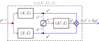
Figure 5: Regret circuit for the convex hull $\mathop{{\rm co}}\{{\cal X},{\cal Y}\}$. The loss function $\ell^{t}_{\lambda}$ is defined in Equation (5).

Extending to multiple set. The construction shown in Figure 5 can be extended to handle the convex hull $\mathop{{\rm co}}\{{\cal X}_{1},\dots,{\cal X}_{n}\}$ of $n$ sets as follows. First, the input loss function $\ell^{t-1}$ is fed into all the $({\cal X}_{i},{\cal L})$-regret minimizers ($i=1,\dots,n$). Then, the loss function $\ell_{\lambda}^{t}$, defined as

$$\ell_{\lambda}^{t}:\Delta^{n}\ni(\lambda_{1},\dots,\lambda_{n})\mapsto\lambda_{1}x_{1}^{t}+\dots+\lambda_{n}x_{n}^{t},$$

is input into a $(\Delta^{n},{\cal L})$-regret minimizer, where $\Delta^{n}$ is the $n$-dimensional simplex. Finally, at each time instant $t$, the $n$ decisions $x_{1}^{t},\dots,x_{n}^{t}$ output by the $({\cal X}_{i},{\cal L})$-regret minimizers are combined with the decision $\lambda^{t}$ output by the $(\Delta^{n},{\cal L})$-regret minimizer to form $\lambda^{t}_{1}x_{1}^{t}+\dots+\lambda_{n}^{t}x_{n}^{t}$.

$V$-polytopes. Our construction can be directly applied to construct an $({\cal X},{\cal L})$-regret minimizer for a $V$-polytope ${\cal X}=\mathop{{\rm co}}\{v_{1},\dots,v_{n}\}$ where $v_{1},\dots,v_{n}$ are $n$ points in a Euclidean space $E$. Of course, any $(\{v_{i}\},{\cal L})$-regret minimizer outputs the constant decision $v_{i}$. Hence, our construction (Figure 5) reduces to a single $(\Delta^{n},{\cal L})$-regret minimizer that observes the (linear) loss function

$$\ell_{\lambda}^{t}:\Delta^{n}\ni(\lambda_{1},\dots,\lambda_{n})\mapsto\lambda_{1}\ell^{t}(v_{1})+\dots+\lambda_{n}\ell^{t}(v_{n}).$$

The observation that a regret minimizer over a simplex can be used to minimize regret over a $V$-polytope already appeared in Zinkevich (2003) and Farina et al. (2017, Theorem 3).

5 Application: Derivation of CFR

We now show that these constructions can be used to construct the CFR framework. The first thing to note is that the strategy space of a single player in an EFG is a treeplex, which can be viewed recursively as a series of convex hull and Cartesian product operations. This perspective is also used when constructing distance functions for first-order methods for EFGs (Hoda et al., 2010; Kroer et al., 2015; 2018). In particular, an information set is viewed as an $n$-dimensional convex hull (since the sum of probabilities over actions is $1$), where each action $a$ at the information set corresponds to a treeplex ${\cal X}_{a}$ representing the set of possible information sets coming after $a$ (in order to perform the convex hull operation, we create a new, larger representation of ${\cal X}_{a}$ so that the dimension is the same for all $a$, described in detail below). The Cartesian product operation is used to represent multiple potential information sets being arrived at (for example different hands dealt in a poker game).

Figure 6 shows an example. Each information set $X_{i}$ (except $X_{0}$) corresponds to a $2$-dimensional convex hull over two treeplexes, one of which is always empty (that is, a leaf node). Each is a Cartesian product. The top-most represents the three possible hands that the player may have when making their first decision. The second layer of Cartesian products represent actions taken by the opponent.

The information-set construction is as follows: let $I$ be the information set under construction, and $A_{I}$ the set of actions. Each action $a\in A_{I}$ has some, potentially empty, treeplex ${\cal X}_{a}$ beneath it; let $n_{a}$ be the dimension of that treeplex. We cannot form a convex hull over $\{{\cal X}_{a}\}_{a\in A_{I}}$ directly since the sets are not of the same dimension, and we do not wish to average across different strategy spaces. Instead, we create a new convex set ${\cal X}_{a}^{\prime}\in{\mathbb{R}}^{|A_{I}|+\sum_{a\in A_{I}}n_{a}}$ for each $a$. The first $|A_{I}|$ indices correspond to the actions in $A_{I}$, and each ${\cal X}_{a}$ gets its own subset of indices. For each $x\in{\cal X}_{a}$ there is a corresponding $x^{\prime}\in{\cal X}_{a}^{\prime}$; $x^{\prime}$ has a $1$ at the index of $a$, $x$ at the indices corresponding to ${\cal X}_{a}$, and $0$ everywhere else. The convex hull is constructed over the set $\{{\cal X}_{a}^{\prime}\}_{a}$, which gives exactly the treeplex rooted at $I$. The Cartesian product is easy and can be done over a given set of treeplexes rooted at information sets $I_{1},\ldots,I_{n}$. The inductive construction rules for the treeplex are given in Figure 7. In fact, one can prove that the $\ell_{\lambda}$ loss functions defined in Equation (5) are exactly the counterfactual loss functions defined in the original CFR paper Zinkevich et al. (2007). If we use as our loss function the gradient $Ay^{t}$ where $y^{t}$ is the opponent’s strategy at iteration $t$, and then apply our expressions for the Cartesian-product and convex-hull regrets inductively, it follows from (5) that the loss function associated with each action is exactly the negative counterfactual value. Finally, the average treeplex strategy as per Theorem 1 coincides with the per-information-set averaging used in standard CFR expositions (e.g., (Zinkevich et al., 2007)).

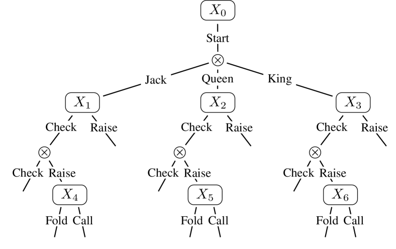
Figure 6: Treeplex for the first player in the game of Kuhn poker. Each $X_{i}$ represents a convex hull over the treeplexes below, while denotes the Cartesian product operation.

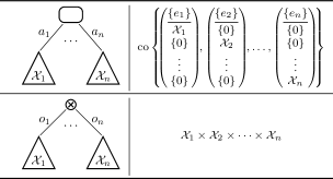
Figure 7: Inductive treeplex construction rules. $e_{i}\in\mathbb{R}^{n}$ contains a 1 at index $i$, and 0 everywhere else.

6 Circuit Construction for Operations that Constrain Sets

Unlike Section 4, in this section we deal with operations that curtail the set of decisions that can be output by our regret minimizer. Section 6.1 and 6.2 propose two different constructions, and Section 6.3 discusses the merits and drawbacks of the two.

6.1 Constraint Enforcement via Lagrangian Relaxation

Suppose that we want to construct an $({\cal X}\cap\{x:g(x)\!\leq\!0\},{\cal L})$-regret minimizer, where $g$ is a convex function, but we only possess an $({\cal X},{\cal L})$-regret minimizer. One natural idea is to use the latter to approximate the former, by penalizing any choice of $x\in{\cal X}$ such that $g(x)>0$. In particular, it seems natural to introduce the penalized loss function

$$\tilde{\ell}^{t}:{\cal X}\ni x\mapsto\ell^{t}(x)+\beta^{t}\max\{0,g(x)\},$$

where $\beta^{t}$ is a (large) positive constant that can change over time. This approach is reminiscent of Lagrangian relaxation. The loss function $\tilde{\ell}^{t}$ is not linear, and as such it cannot be handled as is by our $({\cal X},{\cal L})$-regret minimizer. However, as we have observed in Section 2.1, the regret induced by $\tilde{\ell}^{t}$ can be minimized by our $({\cal X},{\cal L})$-regret minimizer if that observes the “linearized” loss function

$$\tilde{\ell}_{\diamond}^{t}:{\cal X}\ni x\mapsto\ell^{t}(x)+\beta_{\diamond}^{t}\langle\partial g(x^{t}),x\rangle,\qquad$$

where $$\beta_{\diamond}^{t}\mathrel{:\mkern-0.25mu=}\begin{cases}\beta^{t}&\text{if }g(x^{t})>0\\[-2.84526pt] 0&\text{otherwise}.\end{cases}$$

Figure 8 shows the regret circuit corresponding to the construction described so far.

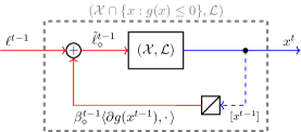
Figure 8: Regret circuit for the Lagrangian relaxation construction (Section 6.1) for the constrained set ${\cal X}\cap\{x:g(x)\leq 0\}$.

In the rest of this subsection we analyze in what sense small cumulative regret implies that the constraint $g(x)\leq 0$ is satisfied. Let $R_{({\cal X},{\cal L})}^{T}$ be the cumulative regret of our $({\cal X},{\cal L})$-regret minimizer. Introducing ${\cal X}_{g}\mathrel{:\mkern-0.25mu=}{\cal X}\cap\{x:g(x)\leq 0\}$ and $\tau_{g}\mathrel{:\mkern-0.25mu=}\{t\in\{1,\dots,T\}:g(x^{t})\!>\!0\}$,

$$R_{({\cal X},{\cal L})}^{T} =\sum_{t=1}^{T}\tilde{\ell}_{\diamond}^{t}(x^{t})-\min_{\hat{x}\in{\cal X}}\left\{\sum_{t=1}^{T}\tilde{\ell}_{\diamond}^{t}(\hat{x})\right\}$$

$$\geq\sum_{t=1}^{T}\ell^{t}(x^{t})+\sum_{t\in\tau_{g}}\beta^{t}g(x^{t})$$

$$\hskip 26.17648pt-\min_{\hat{x}\in{\cal X}}\left\{\sum_{t=1}^{T}\ell^{t}(\hat{x})\!+\!\left(\sum_{t=1}^{T}\beta_{i}\!\right)\!\max\{0,g(\hat{x})\}\!\right\}$$

$$\geq\left(\sum_{t=1}^{T}\ell^{t}(x^{t})\!-\!\min_{\hat{x}\in{\cal X}_{g}}\sum_{t=1}^{T}\ell^{t}(\hat{x})\!\right)\!+\!\!\sum_{t\in\tau_{g}}\beta^{t}g(x^{t}),$$ (6)

where the first inequality is by (2) and the second inequality comes from simply restricting the domain of the minimization from ${\cal X}$ to ${\cal X}_{g}$. Thus, if the $\beta^{t}$ are sufficiently large, the average decision $\bar{x}\mathrel{:\mkern-0.25mu=}\frac{1}{B}(\beta^{1}x^{1}+\dots+\beta^{T}x^{T})$ where $B\mathrel{:\mkern-0.25mu=}\beta^{1}+\dots+\beta^{T}$ satisfies

$$\max\{0,g\}(\bar{x}) \leq\frac{1}{B}\sum_{t=1}^{T}\beta^{t}\max\{0,g\}(x^{t})=\frac{1}{B}\sum_{t\in\tau_{g}}\beta^{t}g(x^{t})$$

$$\leq\frac{1}{B}\!\left(\!R_{({\cal X},{\cal L})}^{T}+\min_{\hat{x}\in{\cal X}_{g}}\left\{\sum_{t=1}^{T}\ell^{t}(\hat{x}-x^{t})\!\right\}\!\right)\!,$$

where the first inequality follows by convexity of $\max\{0,g\}$, and the second inequality follows by (6).

If $\sum_{t=1}^{T}\beta_{i}\gg TLD$, where $L$ is an upper bound on the norm of the loss functions $\ell^{1},\dots,\ell^{T}$ and $D$ is an upper bound on the diameter of ${\cal X}$, then $\max\{0,g(\bar{x})\}\to 0$ as $T\to\infty$, that is, the constraint is satisfied at least by the average in the limit. If $L$ and $D$ are known ahead of time, one practical way to guarantee $\sum_{t=1}^{T}\beta_{i}\gg TLD$ is to choose $\beta^{t}=\kappa LD$ where $\kappa>0$ is a large constant. This guarantees that in the limit, small cumulative regret implies that the average strategy approximately satisfies the constraint and satisfies Hannan consistency. Formally:

Theorem 2.

The decisions $\{x^{t}\}$ produced by a regret minimizer that observes loss functions $\{{\tilde{\ell}}^{t}_{\diamond}\}$ where $\beta^{t}=\kappa LD$ satisfy the following two properties:

• Approximate feasibility: $\displaystyle g\!\left(\frac{1}{T}\sum_{t=1}^{T}x^{t}\right)\leq\frac{1}{\kappa}+o(1).$

• Hannan consistency with respect to {$\ell^{t}$}:

  $$\sum_{t=1}^{T}\ell^{t}(x^{t})\!-\!\min_{\hat{x}\in{\cal X}_{g}}\left\{\sum_{t=1}^{T}\ell^{t}(\hat{x})\right\}=o(T).$$

Alternatively, the $\beta^{t}$ can be chosen by a regret minimizer which sees the constraint violation $\max\{0,g(x^{t})\}$ at time $t$ as its loss function.

6.2 Intersection with a Closed Convex Set

In this subsection we consider constructing an $({\cal X}\cap{\cal Y},{\cal L})$-regret minimizer from an $({\cal X},{\cal L})$-regret minimizer, where ${\cal Y}$ is a closed convex set such that ${\cal X}\cap{\cal Y}\neq\emptyset$. As it turns out, this is always possible, and can be done by letting the $({\cal X},{\cal L})$-regret minimizer give decisions in ${\cal X}$, and then projecting them onto the intersection ${\cal X}\cap{\cal Y}$.

We will use a Bregman divergence $\displaystyle D(y\|x)\mathrel{:\mkern-0.25mu=}d(y)-d(x)-\langle\nabla d(x),y-x\rangle$ as our notion of (generalized) distance between the points $x$ and $y$, where the distance generating function (DGF) $d$ is $\mu$-strongly convex and $\beta$-smooth (that is, $d$ is differentiable and its gradient is Lipschitz continuous with Lipschitz constant $\beta$). Our construction makes no further assumptions on $d$, so the most appropriate DGF can be used for the application at hand. When $d(x)=\|x\|_{2}^{2}$ we obtain $D(x\|y)=\|x-y\|_{2}^{2}$, so we recover the usual Euclidean distance between $x$ and $y$. In accordance with our generalized notion of distance, we define the projection of a point $x\in{\cal X}$ onto ${\cal X}\cap{\cal Y}$ as $\displaystyle\pi_{{\cal X}\cap{\cal Y}}(x)=\mathop{\rm argmin}_{y\in{\cal X}\cap{\cal Y}}D(y\|x).$ For ease of notation, we will denote the projection of $x$ onto ${\cal X}\cap{\cal Y}$ as $[x]$; since ${\cal X}\cap{\cal Y}$ is closed and convex, and since $D(\cdot\|x)$ is strongly convex, such projection exists and is unique. As usual, the cumulative regret of the $({\cal X}\cap{\cal Y},{\cal L})$-minimizer is

$$R_{({\cal X}\cap{\cal Y},{\cal L})}^{T} \!=\sum_{t=1}^{T}\ell^{t}([x^{t}])-\min_{\hat{x}\in{\cal X}\cap{\cal Y}}\left\{\sum_{t=1}^{T}\ell^{t}(\hat{x})\right\}$$

$$\!=\sum_{t=1}^{T}\ell^{t}([x^{t}]\!-\!x^{t})-\!\!\min_{\hat{x}\in{\cal X}\cap{\cal Y}}\!\left\{\sum_{t=1}^{T}\ell^{t}(\hat{x}\!-\!x^{t})\!\right\}\!\!,$$ (7)

where the second equality holds by linearity of $\ell^{t}$. The first-order optimality condition for the projection problem is

$$\langle\nabla d(x^{t})-\nabla d([x^{t}]),\hat{x}-[x^{t}]\rangle\leq 0\quad\forall\,\hat{x}\in{\cal X}\cap{\cal Y}.$$

Consequently, provided $\alpha^{t}\geq 0$ for all $t$,

$$\min_{\hat{x}\in{\cal X}\cap{\cal Y}}\left\{\sum_{t=1}^{T}\ell^{t}(\hat{x}-x^{t})\right\}\geq\min_{\hat{x}\in{\cal X}}\left\{\sum_{t=1}^{T}\ell^{t}(\hat{x}-x^{t})\right.$$

$$\hskip 45.52458pt+\sum_{t=1}^{T}\alpha^{t}\langle\nabla d(x^{t})-\nabla d([x^{t}]),\hat{x}-[x^{t}]\rangle\!\Bigg{\}}.$$ (8)

The role of the $\alpha^{t}$ coefficients is to penalize choices of $x^{t}$ that are in ${\cal X}\setminus{\cal Y}$. In particular, if

$$\frac{1}{\mu}\sum_{t=1}^{T}\ell_{t}([x^{t}]-x^{t})\leq\sum_{t=1}^{T}\alpha^{t}\|[x^{t}]-x^{t}\|^{2},$$ (9)

then, by $\mu$-strong convexity of $d$, we have

$$\sum_{t=1}^{T}\ell_{t}([x^{t}]\!-\!x^{t})\leq\sum_{t=1}^{T}\alpha^{t}\langle\nabla d(x^{t})\!-\!\nabla d([x^{t}]),x^{t}\!-\![x^{t}]\rangle.$$ (10)

Substituting (10) and (8) into Equation (7) we get

$$R_{({\cal X}\cap{\cal Y},{\cal L})}^{T}\leq\left(\sum_{t=1}^{T}\ell^{t}(x^{t})+\alpha^{t}\langle\nabla d(x^{t})-\nabla d([x^{t}]),x^{t}\rangle\right)$$

$$\hskip 39.83368pt-\min_{\hat{x}\in{\cal X}}\left\{\sum_{t=1}^{T}\ell^{t}(\hat{x})+\alpha^{t}\langle\nabla d(x^{t})-\nabla d([x^{t}]),\hat{x}\rangle\!\right\}\!\!,$$

which is the regret observed by an $({\cal X},{\cal L})$-regret minimizer that at each time $t$ observes the linear loss function

$${\tilde{\ell}}^{t}:x\mapsto\ell^{t}(x)+\alpha^{t}\langle\nabla d(x^{t})-\nabla d([x^{t}]),x\rangle.$$ (11)

Hence, as long as condition (9) holds, the regret circuit of Figure 9 is guaranteed to be Hannan consistent.

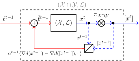
Figure 9: Regret circuit representing the construction of an $({\cal X}\cap{\cal Y},{\cal L})$-regret minimizer using a $({\cal X},{\cal L})$-regret minimizer.

On the other hand, condition (9) can be trivially satisfied by the deterministic choice

$$\alpha^{t}=\begin{cases}0&\text{if }x^{t}\in{\cal X}\cap{\cal Y}\\[5.69054pt] \max\left\{0,\displaystyle\frac{\ell^{t}([x^{t}]-x^{t})}{\mu\|[x^{t}]-x^{t}\|^{2}}\right\}&\text{otherwise}.\end{cases}$$

The fact that $\alpha_{t}$ can be arbitrarily large (when $x^{t}$ and $[x^{t}]$ are very close) is not an issue. Indeed, $\alpha^{t}$ is only used in $\tilde{\ell}^{t}$ (Equation 11) and is always multiplied by a term whose magnitude grows proportionally with the distance between $x^{t}$ and $[x^{t}]$. In fact, the norm of the functional $\tilde{\ell}^{t}$ is bounded:

$$\|\tilde{\ell}^{t}\| \leq\|\ell^{t}\|+\left|\frac{\ell^{t}([x^{t}]-x^{t})}{\mu\|[x^{t}]-x^{t}\|^{2}}\right|\cdot\|\nabla d(x^{t})-\nabla d([x^{t}])\|$$

$$\leq\|\ell^{t}\|+\beta\left|\frac{\ell^{t}([x^{t}]-x^{t})}{\mu\|[x^{t}]-x^{t}\|^{2}}\right|\cdot\|[x^{t}]-x^{t}\|$$

$$\leq\frac{\beta(1+\mu)}{\mu}\|\ell^{t}\|,$$

where the second inequality follows by $\beta$-smoothness of $d$. In other words, our construction dilates the loss functions by at most a factor $\beta(1+\mu)/\mu$.

6.3 Comparison of the Two Constructions

As we pointed out, the decisions in the construction using Lagrangian relaxation only converge to the constrained domain ${\cal X}_{g}$ on average. Thus, formally the construction does not provide an $({\cal X}_{g},{\cal L})$-regret minimizer, but only an approximate one. Section 6.2 solves this problem by providing a generic construction for an $({\cal X}\cap{\cal Y},{\cal L})$-regret minimizer, a strictly more general task. The price to pay is the need for (generalized) projections, a potentially expensive operation. Thus, the choice of which construction to use reduces to a tradeoff between the computational cost of projecting and the need to have exact versus approximate feasibility with respect to $g$. The right choice depends on the application at hand. Finally, the construction based on Lagrangian relaxation requires large penalization factors $\beta^{t}$ in order to work properly. Therefore, the norm of $\tilde{\ell}_{\diamond}^{t}$ can be large, which can complicate the task of minimizing the regret $R_{({\cal X},{\cal L})}^{T}$.

7 Application:​ Handling Strategy Constraints

When solving EFGs, there may be a need to add additional constraints beyond simply computing feasible strategies:

• Opponent modeling. Upon observing repeated play from an opponent, we may wish to constrain our model of their strategy space to reflect such observations. Since observations can be consistent with several information sets belonging to the opponent, this requires adding constraints that span across information sets.

• Bounding probabilities. For example, in a patrolling game we may wish to ensure that a patrol returns to its base at the end of the game with high probability.

• Nash equilibrium refinement computation. Refinements can be computed, or approximated, via perturbation of the strategy space of each player. For extensive-form perfect equilibrium this can be done by lower-bounding the probability of each action at each information set (Farina & Gatti, 2017), which can be handled with small modifications to standard CFR or first-order methods (Farina et al., 2017; Kroer et al., 2017). However, quasi-perfect equilibrium requires perturbations on the probability of sequences of action (Miltersen & Sørensen, 2010), which requires strategy constraints that cross information sets.

All the applications above potentially require adding strategy space constraints that span across multiple information sets. Such constraints break the recursive nature of the treeplex, and are thus not easily incorporated into standard regret-minimization or first-order methods for EFG solving. Davis et al. (2019) propose a Lagrangian relaxation approach called Constrained CFR (CCFR): each strategy constraint is added to the objective with a Lagrangian multiplier, and a regret minimizer is used to penalize violation of the strategy constraints. They prove that if the regret minimizer for the Lagrange multipliers has the optimal Lagrangian multipliers as part of their strategy space, the average output strategy converges to an approximate solution to the constrained game. They also prove a bound on the approximate feasibility of the average output strategy when their algorithm is instantiated with Regret Matching Hart & Mas-Colell (2000) as the local regret minimizer at each information set.

At least two alternative variants of CFR for EFGs with strategy constraints can be obtained using our framework. First, we can apply our method for Lagrangian relaxation of ${\cal X}$ and a constraint $g(x)\leq 0$. Our Lagrangian approach yields as a special case the CCFR algorithm. Our approach supports regret minimization for the Lagrangian multipliers, as was done in CCFR, since we put no constraints on the form of the $\beta^{t}$ multipliers. However, our approach is more general in that it also allows instantiation with a fixed choice of multipliers, thus obviating the need for regret minimization. The second alternative is to apply our construction for the intersection of convex sets (Section 6.2), which uses (generalized) projection onto ${\cal X}\cap\{x:g(x)\leq 0\}$. This leads to a different regret-minimization approach, which has the major advantage that all iterates are feasible, whereas Lagrangian approaches only achieve approximate feasibility. The cost of projection may be nontrivial, and so in general the choice of method depends on the application at hand.

8 Conclusion and Future Research

We developed a calculus of regret minimization, which enables the construction of regret minimizers for composite convex sets that can be inductively expressed as a series of convexity-preserving operations on simpler sets. We showed that our calculus can be used to construct the CFR algorithm directly, as well as several of its variants for the more general case where we have strategy constraints. Our regret calculus is much more broadly applicable than just EFGs: it applies to any setting where the decision space can be expressed via the convexity-preserving operations that we support. In the future we plan to investigate novel applications of our regret calculus. One potential application would be online portfolio selection with additional constraints (e.g., exposure constraints across industries); our framework makes it easy to construct such a regret minimizer from any standard online-portfolio-selection algorithm.

The approach presented in this paper has a large number of potential future applications. For one, it would be interesting to apply our approaches of including additional constraints to the computation of quasi-perfect equilibria. Currently the only solver that is fairly scalable is based on an exact, monolithic, custom approach that uses heavy-weight operations such as matrix inversion, etc. (Farina et al., 2018). Our regret-minimization approach would be the first of its kind for equilibrium refinement that requires constraints that cut across information sets. It obviates the need for the heavy-weight operations, and would still converge to a feasible solution that satisfies an approximate notion of quasi-perfect equilibrium. It would be interesting to study this tradeoff between speed and solution quality.

References

- Bowling et al. (2015) Bowling, M., Burch, N., Johanson, M., and Tammelin, O. Heads-up limit hold’em poker is solved. Science, 347(6218), January 2015.
- Boyd & Vandenberghe (2004) Boyd, S. and Vandenberghe, L. Convex Optimization. Cambridge University Press, 2004.
- Brown & Sandholm (2014) Brown, N. and Sandholm, T. Regret transfer and parameter optimization. In AAAI Conference on Artificial Intelligence (AAAI), 2014.
- Brown & Sandholm (2015a) Brown, N. and Sandholm, T. Regret-based pruning in extensive-form games. In Proceedings of the Annual Conference on Neural Information Processing Systems (NIPS), 2015a.
- Brown & Sandholm (2015b) Brown, N. and Sandholm, T. Simultaneous abstraction and equilibrium finding in games. In Proceedings of the International Joint Conference on Artificial Intelligence (IJCAI), 2015b.
- Brown & Sandholm (2016) Brown, N. and Sandholm, T. Strategy-based warm starting for regret minimization in games. In AAAI Conference on Artificial Intelligence (AAAI), 2016.
- Brown & Sandholm (2017a) Brown, N. and Sandholm, T. Reduced space and faster convergence in imperfect-information games via pruning. In International Conference on Machine Learning (ICML), 2017a.
- Brown & Sandholm (2017b) Brown, N. and Sandholm, T. Safe and nested subgame solving for imperfect-information games. In Proceedings of the Annual Conference on Neural Information Processing Systems (NIPS), pp. 689–699, 2017b.
- Brown & Sandholm (2017c) Brown, N. and Sandholm, T. Superhuman AI for heads-up no-limit poker: Libratus beats top professionals. Science, pp. eaao1733, Dec. 2017c.
- Brown & Sandholm (2019) Brown, N. and Sandholm, T. Solving imperfect-information games via discounted regret minimization. In AAAI Conference on Artificial Intelligence (AAAI), 2019.
- Brown et al. (2017) Brown, N., Kroer, C., and Sandholm, T. Dynamic thresholding and pruning for regret minimization. In AAAI Conference on Artificial Intelligence (AAAI), 2017.
- Burch et al. (2014) Burch, N., Johanson, M., and Bowling, M. Solving imperfect information games using decomposition. In AAAI Conference on Artificial Intelligence (AAAI), 2014.
- Davis et al. (2019) Davis, T., Waugh, K., and Bowling, M. Solving large extensive-form games with strategy constraints. In AAAI Conference on Artificial Intelligence (AAAI), 2019.
- Farina & Gatti (2017) Farina, G. and Gatti, N. Extensive-form perfect equilibrium computation in two-player games. In AAAI Conference on Artificial Intelligence (AAAI), 2017.
- Farina et al. (2017) Farina, G., Kroer, C., and Sandholm, T. Regret minimization in behaviorally-constrained zero-sum games. In International Conference on Machine Learning (ICML), 2017.
- Farina et al. (2018) Farina, G., Gatti, N., and Sandholm, T. Practical exact algorithm for trembling-hand equilibrium refinements in games. In Conference on Neural Information Processing Systems (NeurIPS), 2018.
- Farina et al. (2019) Farina, G., Kroer, C., and Sandholm, T. Online convex optimization for sequential decision processes and extensive-form games. In AAAI Conference on Artificial Intelligence (AAAI), 2019.
- Ganzfried & Sandholm (2015) Ganzfried, S. and Sandholm, T. Endgame solving in large imperfect-information games. In International Conference on Autonomous Agents and Multi-Agent Systems (AAMAS), 2015. Early version in AAAI-13 Workshop on Computer Poker and Incomplete Information.
- Grant et al. (2006) Grant, M., Boyd, S., and Ye, Y. Disciplined convex programming. In Global optimization, pp. 155–210. Springer, 2006.
- Grant et al. (2008) Grant, M., Boyd, S., and Ye, Y. Cvx: Matlab software for disciplined convex programming, 2008.
- Hart & Mas-Colell (2000) Hart, S. and Mas-Colell, A. A simple adaptive procedure leading to correlated equilibrium. Econometrica, 68:1127–1150, 2000.
- Hoda et al. (2010) Hoda, S., Gilpin, A., Peña, J., and Sandholm, T. Smoothing techniques for computing Nash equilibria of sequential games. Mathematics of Operations Research, 35(2), 2010.
- Kroer et al. (2015) Kroer, C., Waugh, K., Kılınç-Karzan, F., and Sandholm, T. Faster first-order methods for extensive-form game solving. In Proceedings of the ACM Conference on Economics and Computation (EC), 2015.
- Kroer et al. (2017) Kroer, C., Farina, G., and Sandholm, T. Smoothing method for approximate extensive-form perfect equilibrium. In Proceedings of the International Joint Conference on Artificial Intelligence (IJCAI), 2017.
- Kroer et al. (2018) Kroer, C., Waugh, K., Kılınç-Karzan, F., and Sandholm, T. Faster algorithms for extensive-form game solving via improved smoothing functions. Mathematical Programming, pp. 1–33, 2018.
- Lanctot et al. (2009) Lanctot, M., Waugh, K., Zinkevich, M., and Bowling, M. Monte Carlo sampling for regret minimization in extensive games. In Proceedings of the Annual Conference on Neural Information Processing Systems (NIPS), 2009.
- Ling et al. (2018) Ling, C. K., Fang, F., and Kolter, J. Z. What game are we playing? End-to-end learning in normal and extensive form games. In Proceedings of the International Joint Conference on Artificial Intelligence (IJCAI), 2018.
- McMahan (2011) McMahan, B. Follow-the-regularized-leader and mirror descent: Equivalence theorems and l1 regularization. In International Conference on Artificial Intelligence and Statistics (AISTATS), pp. 525–533, 2011.
- Miltersen & Sørensen (2010) Miltersen, P. B. and Sørensen, T. B. Computing a quasi-perfect equilibrium of a two-player game. Economic Theory, 42(1), 2010.
- Moravcik et al. (2016) Moravcik, M., Schmid, M., Ha, K., Hladik, M., and Gaukrodger, S. Refining subgames in large imperfect information games. In AAAI Conference on Artificial Intelligence (AAAI), 2016.
- Moravčík et al. (2017) Moravčík, M., Schmid, M., Burch, N., Lisý, V., Morrill, D., Bard, N., Davis, T., Waugh, K., Johanson, M., and Bowling, M. Deepstack: Expert-level artificial intelligence in heads-up no-limit poker. Science, 356(6337), May 2017.
- Tammelin et al. (2015) Tammelin, O., Burch, N., Johanson, M., and Bowling, M. Solving heads-up limit Texas hold’em. In Proceedings of the 24th International Joint Conference on Artificial Intelligence (IJCAI), 2015.
- von Stengel (1996) von Stengel, B. Efficient computation of behavior strategies. Games and Economic Behavior, 14(2):220–246, 1996.
- Zinkevich (2003) Zinkevich, M. Online convex programming and generalized infinitesimal gradient ascent. In International Conference on Machine Learning (ICML), pp. 928–936, Washington, DC, USA, 2003.
- Zinkevich et al. (2007) Zinkevich, M., Bowling, M., Johanson, M., and Piccione, C. Regret minimization in games with incomplete information. In Proceedings of the Annual Conference on Neural Information Processing Systems (NIPS), 2007.