Unified Low Complexity Radix-2 Architectures for Time and Frequency-domain GFDM Modem

Abstract

Most of the conventional multicarrier waveforms explicitly or implicitly involve a generalized frequency division multiplexing (GFDM)-based modem as a core part of the baseband processing. Some are based on GFDM with a single prototype filter, e.g. orthogonal frequency division multiplexing (OFDM) and others employ multiple filters such as filter bank multicarrier (FBMC). Moreover, the GFDM degrees of freedom combined with multiple prototype filters design allow the development and optimization of new waveforms. Nevertheless, GFDM has been widely considered as a complex modulation because of the requirements of odd number of subcarriers or subsymbols. Accordingly, the current state of the art implementations consume high resources. One solution to reduce the complexity is utilizing radix-2 parameters. Due to the advancement in GFDM filter design, the constraint of using odd parameters has been overcome and radix-2 realization is now possible. In this paper, we propose a unified low complexity architecture that can be reconfigured to provide both time-domain and frequency-domain modulation/demodulation. The design consists of several radix-2 fast Fourier transform (FFT) and memory blocks, in addition to one complex multiplier. Moreover, we provide a unified architecture for the state of the art implementations, which is designed based on direct computation of circular convolution using parallel multiplier chains. As we demonstrate in this work, the FFT-based architecture is computationally more efficient, provides more flexibility, significantly reduces the resource consumption, and achieves similar latency for larger block size.

I Introduction

Multicarrier modulation is proposed as an alternative to single-carrier modulation to enable low complexity receiver design, especially in frequency selective channels [1]. OFDM is the dominant scheme adopted by various standards for wired and wireless systems, such as television and audio broadcasting, DSL, wireless area networks, and 4G mobile communications [2]. The main advantage of OFDM is the low complexity implementation. However, OFDM has well-known problems that limit its usage in various applications [3]. For instance, because of its sensitivity to frequency misalignment, OFDM is not suitable for massive networks, that require asynchronous multiple access in order to get rid of synchronization overhead. The high out-of-band (OOB) emissions of OFDM reduce its efficiency for dynamic spectrum access. Moreover, the high peak-to-average power ratio (PAPR) complicates the radio frequency design and increases the cost when deployed in machine type communications. To tackle these challenges, additional processing techniques on top of OFDM have been suggested. In [4], the OFDM signal is smoothed by means of precoding to reduce the OOB. However, this solution further complicates the system implementation. Other low complex variants such as windowed-OFDM [5], and filtered-OFDM [6] enhance the overall OFDM signal by introducing additional processing after the OFDM modulator. In addition to OFDM and its variants, new modulation techniques are proposed to attain the requirements of new use cases. Some aim at providing very low OOB emissions and resistance to frequency and time misalignments, e.g. FBMC [7], while others target the PAPR reduction, e.g. DFT-spread-OFDM [8]. Furthermore, GFDM as a waveform, is proposed in [9] as an alternative to OFDM to improve the spectral efficiency by reducing the cyclic prefix (CP) overhead of OFDM. One GFDM block can have a duration of several OFDM symbols with one CP rather than employing a CP per each OFDM symbol. On the other hand, GFDM provides more degrees of freedom that allow the design of the waveform depending on the use case. For example, targeting high throughput, the design in [10] considers a periodic Raised-Cosine with high roll-off factor, which is well-localized in the time domain (TD). For smooth transitions between the blocks, the first and last subsymbols are not used for data transmission but rather for carrying pilot symbols. To preserve a cyclic structure that enables frequency domain (FD) equalization, a unique word prefix is inserted at the beginning of the frame. With this configuration, GFDM achieves very low OOB, which reduces the number of guard subcarriers for a given spectrum mask compared to OFDM. As a result, a significant throughput gain is archived. Nevertheless, all these benefits are at the cost of increasing the complexity of the receiver because of sacrificing the orthogonality.

The common thread among all multicarrier techniques is the transmission of data in parallel streams, which are then superimposed to formulate the final signal. Each stream can be seen as a single-carrier modulation with a specific pulse shape. In the state of the art multicarrier systems, the pulse shapes are generated by a shift of the prototype filter in the FD and each stream is denoted as subcarrier. These systems correspond to one-dimensional filter design. For instance, OFDM uses a rectangular pulse shape of length equal to the OFDM symbol duration, while filtered multitone (FMT) employs an optimized pulse shape that is several times longer, where multiple symbols overlap [11]. In addition to an FD shift, a TD shift of the prototype pulse is possible, and refers to the subsymbol concept as introduced by GFDM. Actually, even the multicarrier based on the frequency shift can be reformulated in a GFDM form [12]. On the other hand, some modulation schemes, such as FBMC [13], implicitly employ two prototype pulses. These schemes belong to two-dimensional filter design. The general case is a special form of the multidimensional wave principle introduced by Alfred Fettweis in [14], where the waveform is generated from multiple prototype pulses. As shown in this paper, GFDM appears as a basic building unit of all previously cited multicarrier waveforms and can be used to invent optimized waveforms that employ multiple prototype pulses. Therefore, a low-complex implementation is essential for the development of flexible multicarrier systems.

As we show in this paper, the GFDM modem can be implemented with discrete Fourier transform (DFT) blocks. If the involved DFT sizes are of radix-2 basis, i.e. power of $2$, then DFT can be computed with a FFT algorithm. For example in the famous Cooley-Tukey implementation [15], the input vector of size $N$ is split into two sub-vectors of size $N/2$ with respect to the even and odd indexes. The $N/2$-DFT of each sub-vector is computed using FFT. The $N$-DFT is achieved by combining the DFTs of the sub vectors according to the butterfly diagram with the corresponding twiddle factors. This combination requires $N$ complex multiplications. The recursion is repeated until reaching the size $2$, where $2$-DFT is computed with an addition and a subtraction. Therefore, radix-2 FFT significantly reduces the complexity from ${\mathcal{O}}{(N^{2})}$ to ${\mathcal{O}}{(N\log_{2}N)}$ complex multiplications.

As a consequence of the assumption of real-valued symmetric prototype pulse, it is conventionally considered that the number of subcarriers and subsymbols in GFDM should not be both even number to not degrade the overall performance [16]. This assumption leads to a complicated implementation architecture that considers only one radix-2 parameter. The TD real-time implementation in [17] is based on radix-2 number only for subcarriers, while the FD [18] considers only radix-2 number of subsymbols. CP is usually added to the GFDM block to enable FD channel equalization, which requires an additional DFT transform. When TD modulator and FD demodulator are used, only one additional DFT is needed for the channel equalization. Nevertheless, with the previous assumption, either TD or FD is allowed at the same time. Due to the advancement of filter design [19], the condition of using only odd parameters is no longer necessary. Therefore, rethinking efficient implementation is required.
The proposed low-complex architecture in this paper provides a unified architecture for TD and FD realizations of GFDM modulation and demodulation. This architecture employs several FFT blocks, several memory blocks and only one multiplier, which significantly reduces the required resources for hardware implementation. Additionally, the flexible proposed design enable further extension of GFDM to generate coded OFDM waveforms such as Orthogonal time frequency space modulation (OTFS)[20]. In addition, we review the state of the art GFDM implementations and show that the different TD and FD implementations can actually be realized with another unified architecture. Namely, this design requires two FFT blocks, several parallel chains of complex multipliers and memory blocks.

The remainder of the paper is organized as follows: Section II provides a general representation of multicarrier systems highlighting the importance of GFDM as a building block. Section III proposes an advanced representation of GFDM in order to give a closer insight of its structure. The proposed hardware architecture is introduced in IV. In Section V, we reproduce the state of the art implementations in a unified architecture. Section VI is dedicated for the complexity analysis with respect to software and hardware implementation. Finally, Section VII concludes the paper.

The following notations are used throughout the paper: scalars are represented with italic letters $a$, $A$. Column vectors, matrices are denoted with bold-face letters in lower-case for vectors $\bm{a}$, upper-case for matrices $\bm{A}$. The field of complex numbers is denoted as $\mathbb{C}$ and the finite set as calligraphic face ${\mathcal{A}}$, with $|{\mathcal{A}}|$ is the number of elements. The $(m,n)$-th element of a matrix is given by $\left[\bm{A}\right]_{\left(m,n\right)}$ and the $n$-th column of $\bm{A}$ by $\left[\bm{A}\right]_{\left(:,n\right)}$. We use $\{\cdot\}^{T}$, $\{\cdot\}^{H}$ for matrix transpose, and Hermitian transpose. Moreover, $\bm{a}=\mathrm{vec}\left\{\bm{A}\right\}$ indicates vectorization of $\bm{A}\in\mathbb{C}^{K\times M}$, whereas its inverse operator is expressed by $\mathrm{unvec}_{K\times M}\left\{\bm{a}\right\}$. The symbols $\otimes$ and $\odot$ denote Kronecker and element-wise products. Finally, the modulo-$N$ operation is represented as $<\cdot>_{N}$.

II Multicarrier waveforms overview

In linear multicarrier modulation (MCM), a stream of data symbols is split into $N$ parallel substreams. Let $d_{k,m}$ be the stream corresponding to the $k$-th subcarrier and the $m$-th subsymbol. Assuming $K$ subcarriers and $M$ subsymbols, $N=KM$. Each substream is modulated with a transmitter pulse $g^{(\text{tx})}_{k,m}(t)$. In the conventional MCM techniques, the pulses $\{g^{(\text{tx})}_{k,m}\}$ have finite length $T_{t}$, which enables the definition of finite-length modulated symbol as

$$\small\begin{split}x_{i}^{(\text{tx})}(t)=\sum_{k\in{\mathcal{K}}_{\text{on}}}\sum_{m\in{\mathcal{M}}_{\text{on}}}d_{k,m,i}g^{(\text{tx})}_{k,m}(t),~{}t\in[0,T_{t}],\end{split}$$ (1)

where ${\mathcal{K}}_{\text{on}}$ and ${\mathcal{M}}_{\text{on}}$ denote the sets of active subcarriers and subsymbols. The transmitted signal is generated by multiplexing the individual blocks with spacing interval $T_{s}$, so that $1/T_{s}$ is the data rate per stream,

$$\small\begin{split}x^{(\text{tx})}(t)&=\sum_{i\in\mathbb{N}}x_{i}^{(\text{tx})}(t-iT_{s}).\end{split}$$ (2)

The time difference $T_{o}=T_{t}-T_{s}$ defines an overlapping ($T_{o}>0$) or a guard ($T_{o}\leq 0$) interval between successive blocks. For instance, in typical FBMC [21], the overlapping factor is $4$ which means that $T_{t}=4T_{s}$, and thus $T_{o}=3T_{s}$. In some multicarrier waveforms like OFDM and GFDM, the transmitted block is generated form additional processing on top of a core block $x_{i}(t)$ of duration $T$. These include adding CP and cyclic suffix (CS) overheads of duration $T_{\text{cp}}$ and $T_{\text{cs}}$ respectively, in order to facilitate simple FD channel equalization and compensate for the time offset. Afterwards, windowing or filtering can be applied to reduce OOB. In the case of windowing, a window $w(t)$ of duration $T_{\text{t}}=T+T_{\text{cp}}+T_{\text{cs}}$ is applied such that

$$\small\begin{split}x_{i}^{(\text{tx})}(t)&=w(t)x_{i}(<t-T_{\text{cp}}>_{T}).\end{split}$$ (3)

With filtering the block duration is extended by the filter tail $T_{f}$, i.e. $T_{\text{t}}=T+T_{\text{cp}}+T_{\text{cs}}+T_{f}$. Let $w(t)$ be the filter impulse response, the transmitted block is expressed as

$$\small\begin{split}x_{i}^{(\text{tx})}(t)&=w(t)*x_{i}(<t-T_{\text{cp}}>_{T}).\end{split}$$ (4)

Accordingly, we define core pulses $\{g_{k,m}(t)\}$ of duration $T$, which are used to generate the modulation pulses $\{g^{(\text{tx})}_{k,m}\}$ depending on the windowing or filtering, such that

$$\small g^{(\text{tx})}_{k,m}(t)=w(t)[\cdot~{}\mbox{or}~{}*]g_{k,m}(<t-T_{\text{cp}}>_{T}).$$ (5)

Therefore, the core block can be expressed as

$$\small x_{i}(t)=\sum\limits_{k\in{\mathcal{K}}_{\text{on}}}\sum\limits_{m\in{\mathcal{M}}_{\text{on}}}d_{k,m,i}g_{k,m}(t),t\in[0,T].$$ (6)

II-A Discrete-time representation

Without loss of generality, the discrete-time signal is obtained by the sampling of the continuous-time signal with frequency $F_{s}=\tfrac{N}{T}$. The samples of the core block $x_{i}[n]=x_{i}(\tfrac{n}{F_{s}})$ are given by

$$\small x_{i}[n]=\sum_{m\in{\mathcal{K}}_{\text{on}}}\sum_{m\in{\mathcal{M}}_{\text{on}}}d_{k,m,i}g_{k,m}[n],n=0\cdots N-1.$$ (7)

This linear relation can be reformulated in a matrix form $\bm{x}_{i}=\bm{A}\bm{d}_{i},$ where $\left[\bm{d}_{i}\right]_{\left(k+mK\right)}=d_{k,m,i},~{}(k,m)\in{\mathcal{K}}_{\text{on}}\times{\mathcal{M}}_{\text{on}}$ and $0$ elsewhere. $\bm{A}\in\mathbb{C}^{N\times N}$ is the modulation matrix defined by $\left[\bm{A}\right]_{\left(n,k+mK\right)}=g_{k,m}[n]$.

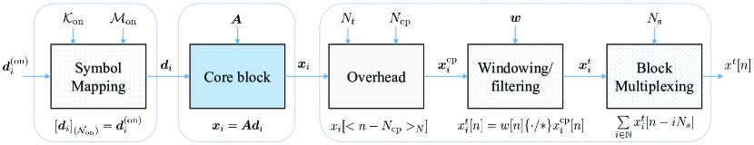
Figure 1: Multicarrier waveforms generator stages.

Based on that, the multicarrier waveform realization can be split into three independent modules as depicted in Fig. 1;

1. Symbol mapping: a vector of data symbols $\bm{d}_{i}^{(\text{on})}\in\mathbb{C}^{|{\mathcal{N}}_{\text{on}}|\times 1}$ is mapped to $\bm{d}_{i}$, such that $\left[\bm{d}_{i}\right]_{\left({\mathcal{N}}_{\text{on}}\right)}=\bm{d}_{i}^{(\text{on})}$, where $\small{\mathcal{N}}_{\text{on}}=\left\{n=k+mK,~{}(k,m)\in{\mathcal{K}}_{\text{on}}\times{\mathcal{M}}_{\text{on}}\right\}.$

2. Core block modulation.

3. Further processing and multiplexing.

The core block implementation is the essential part. In the most general cases it requires $N^{2}$ complex multiplications and a memory to store $N^{2}$ complex coefficients. In practical MCM, the matrix $\bm{A}$ has a well-defined structure based on the design of the pulses $\{{g_{k,m}[n]}\}$ which define the columns of $\bm{A}$. This structure can be exploited in the implementation.

II-B Modulation pulses design

It is common to derive $\{g_{k,m}(t)\}$ from one prototype pulse $g(t)$ by means of shift in the time and frequency domains. Let $\Delta f$, $T_{\text{sub}}$ be the FD subcarrier spacing and TD subsymbol spacing, respectively. Then,

$$\small g_{k,m}(t)=u_{T}(t)g(t-mT_{\text{sub}})e^{j2\pi\Delta fkt}.$$ (8)

where $u_{T}(t)$ is a rectangular window of duration $T$ used to confine the pulse shape in the time duration $T$. In order to preserve the energy per stream, the pulse $g(t)$ needs to be periodic. An explicit periodic prototype pulse is used, e.g. in GFDM and OFDM, whereas FMT [11], which originally defines only subcarriers, can be reformulated to involve subsymbols. The set ${\mathcal{M}}_{\text{on}}$ is determined based on the filter overlapping factor. Under this constraint, we focus on a periodic prototype pulse. For practical implementation, we assume that $Q={T\Delta f}$ and $P={T_{\text{sub}}}F_{s}=\tfrac{N}{T}{T_{\text{sub}}}$ are integer numbers so that

$$\small g_{k,m}[n]=g[<n-mP>_{N}]e^{j2\pi\frac{nkQ}{N}}.$$ (9)

The parameters $Q$ and $P$ denote the subcarrier and subsymbol spacing in samples, respectively (see Fig. 2).

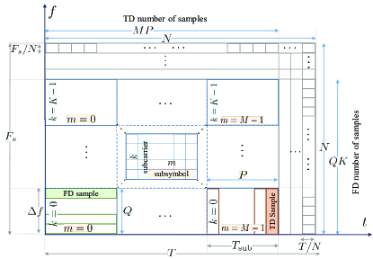
Figure 2: Time-frequency design parameters.

Actually $\{g_{k,m}\}$ belong to Gabor time-frequency lattices [22], with $g_{k\alpha,m\beta}[n]=g[<n-m\beta>_{N}]e^{j2\pi nk\alpha}$, $\alpha=Q/N,~{}\beta=P$. In order to uniquely demodulate the data symbols $d_{k,m}$ from a given $x[n]$, Wexler-Raz duality condition [23] must be satisfied. Thus, there exists a pulse $h[n]$ that attains $\langle h,g_{k/\beta,m/\alpha}\rangle=\alpha\beta\delta_{k,0}\delta_{m,0}$, where $g_{k/\beta,m/\alpha}$ is the dual Gabor lattice, $\delta_{ij}$ refers to Kronecker delta, and $\langle\cdot\rangle$ denotes the inner product. Furthermore, $h$ is the demodulator prototype pulse, such that $d_{k,m}=\langle x,h_{k\alpha,m\beta}\rangle$. It is rigorously proven in [24] that Wexler-Raz duality condition cannot be fulfilled if $\alpha\beta>1$. Based on that the choice of $P$ and $Q$ is influenced by

• $QP\leq N$, which is necessary but not sufficient to achieve Wexler-Raz duality condition.

• $\Delta fK\leq F_{s}=\tfrac{N}{T}$, which is a necessary, but not sufficient condition for the signal to have a bandwidth $B\leq F_{s}$.

Consequently, the design needs to fulfill the conditions

$$\small Q\leq M,~{}P\leq K.$$

It is required for efficient implementation purposes to consider the case $PQ=N$, i.e. $P=K$ and $Q=M$, which correspond to critically sampled system. Essentially, this special case corresponds to GFDM-based system [9]. Fortunately, a system that requires $PQ<N$, i.e. an over-sampled system, can be redesigned to satisfy the condition $PQ=N$ by managing the sampling frequency, the block length, and properly defining the active sets. Accordingly, let $Q=T\Delta f=M$ and $P=T_{\text{sub}}F_{s}=\frac{K}{L}$, where $L$ is a positive integer. The set of active subcarriers ${\mathcal{K}}_{\text{on}}$ is adjusted to the available bandwidth $B\leq F_{s}$. The modulation pulses can be redefined as

$$\small\begin{split}g_{k,mL+l}[n]&=g(<n-mK-l\tfrac{K}{L}>_{N})e^{j2\pi\frac{nkM}{N}}.\end{split}$$

Then, $L$ prototype pulses can be defined by

$$\small g^{(l)}[n]=g[<n-l\tfrac{K}{L}>_{N}],~{}l=0\cdots,L-1.$$

Each pulse shape is used to generate a subset of the pulse shapes with the subsymbol spacing $K$ and the set

$$\small{{\mathcal{M}}_{\text{on}}}^{(l)}=\{mL+l,~{}l\leq mL+l<M\}.$$

The final block can be expressed as superposition of $L$ GFDM-based block $x[n]=\sum_{l=0}^{L-1}x^{(l)}[n]$, where

$$\small x^{(l)}[n]=\sum_{k\in{\mathcal{K}}_{\text{on}}}\sum_{m\in{{\mathcal{M}}_{\text{on}}}^{(l)}}d_{k,m}g^{(l)}[<n-mK>_{N}]e^{j2\pi\frac{nk}{K}}.$$ (10)

An alternative reformulation can be achieved in the frequency domain with respect to the $N$-DFT of ${g}_{k,m}[q]$ given by

$$\tilde{g}_{k,m}[q]=\tilde{g}[<q-kQ>_{N}]e^{-j2\pi\frac{qmP}{N}}.$$ (11)

The design is adjusted such that $P=T_{\text{sub}}F_{s}=K$ and $Q=\tfrac{M}{L}$ resulting in the prototype pulses

$$\tilde{g}^{(l)}[q]=\tilde{g}[<q-l\tfrac{M}{L}>_{N}],~{}l=0\cdots,L-1,$$

for the sets ${{\mathcal{K}}_{\text{on}}}^{(l)}=\{kL+l,~{}l\leq kL+l<K\}$. This approach can be generalized to design a waveform with $L$ prototype pulses $\{g^{(l)}[n]\}$. Each prototype pulse is associated with the sets ${{\mathcal{K}}_{\text{on}}}^{(l)}$ and ${{\mathcal{M}}_{\text{on}}}^{(l)}$, as shown in Fig. 3. Thus, for $(k,m)\in{{\mathcal{K}}_{\text{on}}}^{(l)}\times{{\mathcal{M}}_{\text{on}}}^{(l)}$

$$\small g_{k,m}[n]=g^{(l)}(<n-mK>_{N})e^{j2\pi\frac{nk}{K}}.$$ (12)

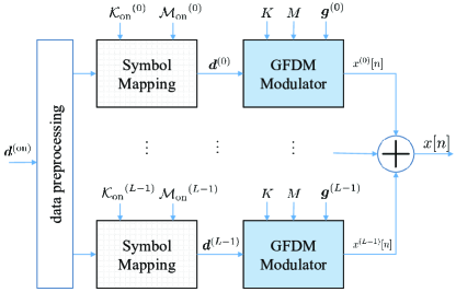
Figure 3: Core block with multiple prototype pulses.

The input data symbol can be preprocessed prior to modulation, for instance to produce offset quadrature amplitude modulation (OQAM) [25]. This design allows the realization of wide range of multicarrier waveforms. For example, to generate FBMC, where $Q=M$ and $P=K/2$, first, the complex QAM data symbols $d_{k,m}=d^{(I)}_{k,m}+jd^{(Q)}_{k,m}$ are split into two OQAM precoded streams, $d^{(0)}_{k,m}=\theta_{0,k}d^{(I)}_{k,m}$, $d^{(1)}_{k,m}=\theta_{1,k}d^{(Q)}_{k,m}$, where

$$\small\theta_{0,k}=\left\{\begin{array}[]{ll}j,&~{}k\mbox{ is even}\\ 1,&~{}k\mbox{ is odd}\end{array}\right\},\theta_{1,k}=\left\{\begin{array}[]{ll}1,&~{}k\mbox{ is even}\\ j,&~{}k\mbox{ is odd}\end{array}\right\}.$$

The streams are then fed to two GFDM modulators with the parameters $g^{(0)}[n]=g[n]$, $g^{(1)}[n]=g[<n-K/2>]$, ${{\mathcal{K}}_{\text{on}}}^{(0)}={{\mathcal{K}}_{\text{on}}}^{(1)}$, and ${{\mathcal{M}}_{\text{on}}}^{(0)}={{\mathcal{M}}_{\text{on}}}^{(1)}$. The output is a superposition of both GFDM blocks, i.e. $x[n]=x^{(0)}[n]+x^{(1)}[n]$.

II-C Relation to multidimensional digital filtering

GFDM can be seen as a circular filtering of data symbols per subcarrier. For simplicity, consider a single carrier system, i.e., $K=1$. From Fig. 3,

$$x[n]=\sum_{l=0}^{L-1}\sum\limits_{m\in{\mathcal{M}}_{\text{on}}^{(l)}}d_{m}^{(l)}g^{(l)}[<n-m>_{N}].$$ (13)

The multidimensional circular filtering can be expressed as

$$\small\begin{split}x[n_{0},\cdots&,n_{L-1}]=\sum_{m_{0}=0}^{M-1}\cdots\sum_{m_{L-1}=0}^{M-1}D_{m_{0},\cdots,m_{L-1}}\\ &\times G[<n_{0}-m_{0}>_{N},\cdots,<n_{L-1}-m_{L-1}>_{N}].\end{split}$$ (14)

Here, $D_{m_{0},\cdots,m_{L-1}}$ corresponds to the multi-dimensional data, while $G[n_{0},\cdots,n_{L-1}]$ is the multidimensional filter. Therefore, GFDM with multiple prototype pulses is a special case, where $D_{m_{0},\cdots,m_{L-1}}$ is sparse with $M$ non-zero values. The multidimensional filter coefficients are set to satisfy (13). Although the work of Alfred Fettweis on multidimensional wave-digital principle [14] targets other applications, it inspires more investigation for wireless communications. In this context, a one-dimensional circular filtering appears in the received signal model of OFDM under frequency selective channel. On the other hand, the received signal of OTFS [20] is modeled as two-dimensional filtering with a time-variant channel response in the delay-Doppler domain. Accordingly, three-dimensional filtering can be a natural candidate when considering the spatial domain. As we show in this paper, a GFDM core can be used to efficiently realize one-dimensional convolution, which is a crucial step for multidimensional filtering.

III GFDM time-frequency representations

TABLE I: Summary of GFDM equations.

	Time domain	Frequency domain
Modulation
Conv.	$\left[\bm{V}^{(\bm{x})}_{M,K}\right]_{\left(p,q\right)}=\sum\limits_{m=0}^{M-1}\left[\bm{V}^{(\bm{g})}_{M,K}\right]_{\left(<p-m>_{M},q\right)}\left[\bm{D}^{T}\bm{F}_{K}^{H}\right]_{\left(m,q\right)}$	$\left[\bm{V}^{(\tilde{\bm{x}})}_{K,M}\right]_{\left(q,p\right)}=\sum\limits_{k=0}^{K-1}\left[\bm{V}^{(\tilde{\bm{g}})}_{K,M}\right]_{\left(<q-k>_{K},p\right)}\left[\bm{D}\bm{F}_{M}\right]_{\left(k,p\right)}$
Zak trans.	${\bm{V}^{(\bm{x})}_{M,K}}=\frac{1}{MK}\bm{F}_{M}^{H}\left(\bm{W}_{\text{tx}}\odot\left[\bm{F}_{K}^{H}{\bm{D}\bm{F}_{M}}\right]\right)^{T}$	${\bm{V}^{(\tilde{\bm{x}})}_{K,M}}=\frac{1}{K}\bm{F}_{K}\left(\bm{W}_{\text{tx}}\odot\left[\bm{F}_{K}^{H}{\bm{D}\bm{F}_{M}}\right]\right)$
Tx win.	$\bm{W}_{\text{tx}}=K{\bm{Z}^{(\bm{g})}_{M,K}}^{T}$	$\bm{W}_{\text{tx}}=K{\bar{\bm{Z}}^{(\tilde{\bm{g}})}_{K,M}}$
Demodulation
Zak trans.	$\hat{\bm{D}}=\frac{1}{M}\bm{F}_{K}\left(\bm{W}_{\text{rx}}\odot\left[\bm{F}_{M}\bm{V}^{({\bm{y}_{\text{eq}}})}_{M,K}\right]^{T}\right)\bm{F}_{M}^{H}$	$\hat{\bm{D}}=\frac{1}{M}\bm{F}_{K}\left(\bm{W}_{\text{rx}}\odot\left[\frac{1}{K}\bm{F}_{K}^{H}\bm{V}^{(\tilde{\bm{y}}_{\text{eq}})}_{K,M}\right]\right)\bm{F}_{M}^{H}$
Conv.	$\small\left[\frac{1}{K}\hat{\bm{D}}^{T}\bm{F}_{K}^{H}\right]_{\left(p,q\right)}=\sum\limits_{m=0}^{M-1}\left[\bm{V}^{(\bar{\bm{\gamma}})}_{M,K}\right]_{\left(<p-m>_{M},q\right)}\left[\bm{V}^{({\bm{y}}_{\text{eq}})}_{M,K}\right]_{\left(m,q\right)}$	$\left[\hat{\bm{D}}\bm{F}_{M}\right]_{\left(q,p\right)}=\frac{1}{K}\sum\limits_{k=0}^{K-1}\left[\bm{V}^{(\bar{\tilde{\bm{\gamma}}})}_{K,M}\right]_{\left(<q-k>_{K},p\right)}\left[\bm{V}^{(\tilde{\bm{y}}_{\text{eq}})}_{K,M}\right]_{\left(k,p\right)}$
Rx win.	$\small\bm{V}^{(\bar{\bm{\gamma}})}_{M,K}=\frac{1}{M}\bm{F}_{M}^{H}\bm{W}_{\text{rx}}^{T}$	$\bm{V}^{(\bar{\tilde{\bm{\gamma}}})}_{K,M}=\bm{F}_{K}\bm{W}_{\text{rx}}$

In this section, we represent GFDM by means of the discrete Zak transform [26]. This reflects the involvement of TD and FD-shifted modulation pulses. It also clarifies the structure and facilitates the implementation. Consider a vector $\bm{a}\in\mathbb{C}^{QP\times 1}$, the polyphase matrix of size $Q\times P$ is defined as

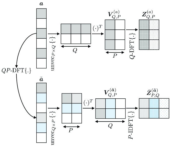
Figure 4: Zak transform.

$$\small\bm{V}^{(\bm{a})}_{Q,P}=\mathrm{unvec}_{P\times Q}\left\{\bm{a}\right\}^{T}\Leftrightarrow\left[\bm{V}^{(\bm{a})}_{Q,P}\right]_{\left(q,p\right)}=\left[\bm{a}\right]_{\left(p+qP\right)}.$$ (15)

The $p$-th column of this matrix results from the sampling of $a[n]$ by factor $P$ with shift $p$, as depicted in Fig. 4. By applying $Q$-DFT on each column we get the discrete Zak transform

$$\small\bm{Z}^{(\bm{a})}_{Q,P}=\bm{F}_{Q}\bm{V}^{(\bm{a})}_{Q,P}\in\mathbb{C}^{Q\times P}.$$ (16)

A dual Zak transform in the frequency domain is obtained for the frequency domain vector $\tilde{\bm{a}}=\bm{F}_{PQ}\bm{a}$ as

$$\small\bar{\bm{Z}}^{(\tilde{\bm{a}})}_{P,Q}=\frac{1}{P}\bm{F}_{P}^{H}\bm{V}^{(\tilde{\bm{a}})}_{P,Q}\in\mathbb{C}^{P\times Q}.$$ (17)

The basic TD-GFDM equation can be reformulated in polyphase form by using two indexes $q=0,\cdots,K-1$ and $p=0\cdots,M-1$, such that $n=+pK$. Thereby,

$$\small\left[\bm{x}\right]_{\left(q+pK\right)} =\sum\limits_{m=0}^{M-1}\sum\limits_{k=0}^{K-1}d_{k,m}g[<q+pK-mK>_{N}]e^{j2\pi\frac{k}{K}q}.$$

Using the polyphase representation given in (15), then

$$\small\begin{split}\left[\bm{V}^{(\bm{x})}_{M,K}\right]_{\left(p,q\right)}&=\sum\limits_{m=0}^{M-1}\left[\bm{V}^{(\bm{g})}_{M,K}\right]_{\left(<p-m>_{M},q\right)}\left[\bm{D}^{T}\bm{F}_{K}^{H}\right]_{\left(m,q\right)}.\end{split}$$ (18)

This defines circular convolution [27] between the $q$-th column of $\bm{V}^{(\bm{g})}_{M,K}$ and the $q$-th column of $\bm{D}^{T}\bm{F}_{K}^{H}$ and it can be expressed in the FD with $M$-DFT as

$$\small\begin{split}\left[\bm{F}_{M}\bm{V}^{(\bm{x})}_{M,K}\right]_{\left(p,q\right)}=\left[\bm{F}_{M}{\bm{V}}_{M,K}^{(\bm{g})}\right]_{\left(q,q\right)}\cdot\left[\bm{F}_{M}\bm{D}^{T}\bm{F}_{K}^{H}\right]_{\left(p,q\right)},\end{split}$$

which corresponds to time-domain Zak transform (19). Thus,

$$\small\begin{split}{\bm{V}^{(\bm{x})}_{M,K}}=\frac{1}{MK}\bm{F}_{M}^{H}\left(K\bm{Z}^{(\bm{g})}_{M,K}\odot\left[\bm{F}_{M}{\bm{D}^{T}\bm{F}_{K}^{H}}\right]\right).\end{split}$$ (19)

The demodulator performs the inverse steps. Let $\bm{y}_{\text{eq}}$ be the TD equalized signal, then

$$\small\hat{\bm{D}}=\frac{1}{M}\bm{F}_{K}\left(\bm{W}_{\text{rx}}\odot\left[\bm{F}_{M}\bm{V}^{({\bm{y}_{\text{eq}}})}_{M,K}\right]^{T}\right)\bm{F}_{M}^{H}.$$

Here $\bm{W}_{\text{rx}}\in\mathbb{C}^{K\times M}$ is the receive window corresponding to the demodulator prototype pulse. Accordingly, the demodulation convolution in the TD is given by

$$\small\left[\frac{1}{K}\hat{\bm{D}}^{T}\bm{F}_{K}^{H}\right]_{\left(p,q\right)}=\sum\limits_{m=0}^{M-1}\left[\bm{V}^{(\bar{\bm{\gamma}})}_{M,K}\right]_{\left(<p-m>_{M},q\right)}\left[\bm{V}^{({\bm{y}}_{\text{eq}})}_{M,K}\right]_{\left(m,q\right)},$$ (20)

where $\small\bm{V}^{(\bar{\bm{\gamma}})}_{M,K}=\frac{1}{M}\bm{F}_{M}^{H}\bm{W}_{\text{rx}}^{T}$. A dual FD representation can be derived in a similar way. Table I summarizes the GFDM modem equations for both TD and FD representations.

IV Proposed GFDM modem architecture

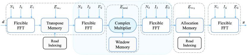
Figure 5: Unified architecture for TD and FD GFDM processing.

Our proposed architecture is developed based on the Zak transform representation of the GFDM samples. The TD representation can be reformulated as

$$\small\begin{split}{\bm{V}^{(\bm{x})}_{M,K}}=\frac{1}{M}\bm{F}_{M}^{H}\left(\bm{W}_{\text{tx}}^{T}\odot\left(\bm{F}_{M}\left[\frac{1}{K}\bm{F}_{K}^{H}\bm{D}\right]^{T}\right)\right),\end{split}$$

and the FD representation can be reformulated as

$$\small\begin{split}{\bm{V}^{(\tilde{\bm{x}})}_{K,M}}=\bm{F}_{K}\left(\bm{W}_{\text{tx}}\odot\left(\frac{1}{K}\bm{F}_{K}^{H}\left[\bm{F}_{M}\bm{D}^{T}\right]^{T}\right)\right).\end{split}$$

Both equations have similar structure with simple differences. In the TD, the data symbols are fed to the modulator by the columns of $\bm{D}$. Then, a $K$-IDFT is computed for each column, and the result of $N$ samples need to be stored in a matrix $\tilde{\bm{D}}$ of size $K\times M$. Afterwards, the samples of $\tilde{\bm{D}}$ are forwarded row-by-row to an $M$-DFT block. The output of the $M$-DFT can be directly element-wise multiplied with the rows of the stored modulation window $\bm{W}_{\text{tx}}$. The result is then fed to an $M$-IDFT block and the output is stored in the columns of the matrix ${\bm{V}^{({\bm{x}})}_{M,K}}$. Finally, the core block is generated by reading ${\bm{V}^{({\bm{x}})}_{M,K}}$ in rows. The FD modulator, works similarly by feeding the data of $\bm{D}$ in rows, and replacing the $K$ by $M$ and the DFT by inverse discrete Fourier transform (IDFT). The resulting FD samples are stored in a matrix ${\bm{V}^{(\tilde{\bm{x}})}_{K,M}}$ and read by rows. Additionally, the FD modulator requires a final $N$-DFT to transform the block to the TD.

The radix-2 values of $K$ and $M$ enables the implementation of DFT with flexible FFT intellectual property (IP) cores, e.g. Xilinx FFT. This core allows the run-time reconfiguration of the size of DFT and setting the block either in DFT or IDFT mode. The proposed architecture is illustrated in Fig. 5. In this design, $4$ flexible FFT cores with the configuration parameter $N_{x}$ for the DFT size and $I_{x}$ to set the core in the direct $[D]$ or inverse $[I]$ mode. Additionally, each FFT block can be enabled $[E]$ or disabled $[D]$ with the parameter $E_{x}$, such that the disabled block forwards the samples to the next stage. The $4$-th FFT core is optional depending on the desired domain of implementation. Moreover, one memory block is used to store the result of the first transform and performs the transpose by the configuration of the indexing unit. The modulator window is stored in a memory as part of the modulator configuration. This memory is always read incrementally and written with respect to the implementation domain. Furthermore, one high throughput complex multiplier is used to perform the element-wise multiplication. A third memory is required to store the samples prior to generating the final block by performing the transpose. All the building blocks can be disabled as well. Actually the highlighted box corresponds to the computation of the convolution. Table II summarize the configuration parameters of the modulator.

TABLE II: Configuration parameters for modulator.

Parameter	TD	FD
$[N_{1},N_{2},N_{3},N_{4}]$	$[K,M,M,-]$	$[M,K,K,N]$
$[I_{1},I_{2},I_{3},I_{4}]$	$[I,D,I,-]$	$[D,I,D,I]$
$[E_{1},E_{2},E_{3},E_{4}]$	$[E,E,E,D]$	$[E,E,E,E]$
Window	$\bm{W}_{\text{tx}}^{T}$	$\bm{W}_{\text{tx}}$
allocation	$\{\cdot\}^{T}$	$\{\cdot\}^{T}$

TABLE III: Demodulator configuration, FD equalization.

Parameter	TD	FD
deallocation	$\mathrm{unvec}_{K\times M}\left\{\cdot\right\}^{T}$	$\mathrm{unvec}_{M\times K}\left\{\cdot\right\}^{T}$
Window	$\bm{W}_{\text{rx}}^{T}$	$\bm{W}_{\text{rx}}$
$[N_{4},N_{3},N_{2},N_{1}]$	$[N,M,M,K]$	$[-,K,K,M]$
$[I_{4},I_{3},I_{2},I_{1}]$	$[I,D,I,D]$	$[-,I,D,I]$
$[E_{4},E_{3},E_{2},E_{1}]$	$[E,E,E,E]$	$[D,E,E,E]$

The demodulator has similar architecture in reversed order. The $N_{4}$-FFT block is enabled or disabled depending on the domain of the equalized signal and the configuration of the demodulator. For instance, if the input is an FD equalized signal and the modulator is configured in TD, this block needs to be configured as $N$-IFFT. The allocation memory is used to store the received signal in columns and forward it in rows to the next block. The samples at the output of the demodulator correspond to the columns of $\hat{\bm{D}}$ in the TD and to the rows in the FD configuration. The demodulator settings with respect to FD equalization are listed in Table III.

Usually, FD equalization is used. Thus, the modem can be configured as TD modulator and FD demodulator. In this way, the overall modulation and equalization processing requires only one $N$-FFT for the equalizer. On the other hand, including $N_{4}$-FFT preserves the symmetry of the architecture. Therefore, with fast reconfiguration, the modulator can be reconfigured as demodulator. This solution is typical for low-cost time division duplex transmission. The bypass function of each block allows faster processing of certain waveforms. For instance, OFDM requires only one IFFT to generate TD samples. DFT-spread-OFDM requires only a single FFT in the FD. Additionally, one or more FFT cores can be disabled for certain precoding methods like in [28]. Furthermore, $N_{4}$-FFT core can be configured with $N_{4}>N$ to produce over-sampled signal. The allocation indexing can be altered to implement sort of frequency division multiple access (FDMA) and multiplex pilot samples. For example, the recent proposed OTFS [20] is generated by disabling the final transpose.

V Unified architecture for the state of the art implementations

TABLE IV: Summary of the settings of the circular convolution architecture.

	Time-domain	Frequency-domain
Modulation
Transform	$K$-IFFT	$M$-FFT
Pulse shape	$\left[\bar{\bm{G}}^{(m)}\right]_{\left(:,p\right)}=K\left[{\bm{V}^{(\bm{g})}_{M,K}}^{T}\right]_{\left(:,<p-m>_{M}\right)}$	$\bar{\bm{G}}^{(l)}=\bm{1}_{1\times K}\otimes\left[{\bm{V}^{(\tilde{\bm{g}})}_{K,M}}^{T}\right]_{\left(:,l\right)}$
Data	$\bar{\bm{D}}^{(m)}=\bm{1}_{1\times M}\otimes\left[\frac{1}{K}\bm{F}_{K}^{H}\bm{D}\right]_{\left(:,m\right)}$	$\left[\bar{\bm{D}}^{(l)}\right]_{\left(:,q\right)}=\left[{\bm{F}_{M}\bm{D}^{T}}\right]_{\left(:,<q-l>_{K}\right)}$
$N$-IDFT	Disabled	Enabled
Demodulation / FD equalization
Pulse shape	$\left[\bar{\bm{\Gamma}}^{(m)}\right]_{\left(:,p\right)}=\left[{\bm{V}^{(\bar{\bm{\gamma}})}_{M,K}}^{T}\right]_{\left(:,<p-m>_{M}\right)}$	$\bar{\bm{\Gamma}}^{(l)}=\frac{1}{K}\bm{1}_{1\times K}\otimes\left[{\bm{V}^{(\bar{\tilde{\bm{\gamma}}})}_{K,M}}^{T}\right]_{\left(:,l\right)}$
Data	$\small\bar{\bm{Y}}^{(m)}=\bm{1}_{1\times M}\otimes\left[{\bm{V}^{({\bm{y}}_{\text{eq}})}_{M,K}}^{T}\right]_{\left(:,m\right)}$	$\left[\bar{\bm{Y}}^{(l)}\right]_{\left(:,q\right)}=\left[{\bm{V}^{(\tilde{\bm{y}}_{\text{eq}})}_{K,M}}^{T}\right]_{\left(:,<q-l>_{K}\right)}$
Transform	$K$-FFT	$M$-IFFT
$N$-IDFT	Enabled	Disabled

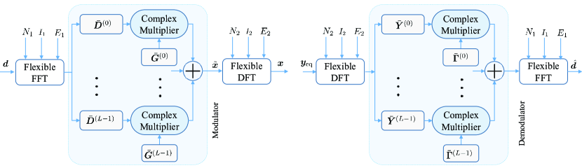
Figure 6: State of the art implementation.

The state of the art methods originally target the implementation of the conventional GFDM waveform, where mostly periodic raised-cosine (RC) prototype pulse with two-subcarrier overlap is used. Accordingly, the structure is influenced by the fact that the parameters $K$ and $M$ cannot be even numbers at the same time for real-valued symmetric pulse [16]. Therefore, to avoid the singularity of the modulation matrix, either $M$ or $K$ need to be odd number. Recently, in [19], a detailed study on the prototype filter provides design rules for selecting the proper pulse, and shows that the periodic pulse can be generated by the sampling of the frequency response of a basic filter. The starting point of the samples influences the condition number of the modulation matrix for certain parameters. For even numbers of $K$ and $M$, the starting point has to be shifted by half the sample. This results in a Hermitian symmetric prototype pulse. Moreover, the performance considering this design rule follows the same trend. For instance, the condition number and the noise enhancement increases with the increase of $M$ for a roll-off factor $\alpha>0$. Based on this restriction, two main methods have been proposed, as described in Section V-A and Section V-B.

V-A TD Implementation

The first method focuses on TD implementation of GFDM modem [17], where $K$ is radix-2 and $M$ is odd. A closer analysis of this architecture shows that this method actually implements the TD convolution

$$\small\begin{split}\left[\bm{V}^{(\bm{x})}_{M,K}\right]_{\left(p,q\right)}&=\sum_{m=0}^{M-1}\left[\bm{V}^{(\bm{g})}_{M,K}\right]_{\left(<p-m>_{M},q\right)}\left[\bm{D}^{T}\bm{F}_{K}^{H}\right]_{\left(m,q\right)}.\end{split}$$

In the first step, the $K$-DFT of the columns of $\bm{D}$ is computed using an IFFT core. In order to exploit parallel processing to reduce latency, the convolution is reformulated in the form

$$\small\{\bm{V}^{(\bm{x})}_{M,K}\}^{T}=\sum_{m=0}^{M-1}\bar{\bm{G}}^{(m)}\odot\bar{\bm{D}}^{(m)},$$ (21)

where $\bar{\bm{D}}^{(m)}$ is used to store $M$ replicas of the DFT of the $m$-th column of $\bm{D}$, and $\{\bar{\bm{G}}^{(m)}\}$ are prestored matrices derived from the prototype pulse. The mathematical details are summarized in Table IV. After the computation of the DFT of the $M$ columns of $\bm{D}$ and storing the results in $\{\bar{\bm{D}}^{(m)}\}$, $M$ complex multipliers work in parallel to element-wise multiply the columns of $\{\bar{\bm{D}}^{(m)}\}$ and $\{\bar{\bm{G}}^{(m)}\}$. The outputs of the multipliers are summed together producing the block samples. The demodulation is performed in a reverse order. The first step is computing the convolution

$$\small\left[\tfrac{1}{K}\hat{\bm{D}}^{T}\bm{F}_{K}^{H}\right]_{\left(p,q\right)}=\sum\limits_{m=0}^{M-1}\left[\bm{V}^{(\bar{\bm{\gamma}})}_{M,K}\right]_{\left(<p-m>_{M},q\right)}\left[\bm{V}^{({\bm{y}}_{\text{eq}})}_{M,K}\right]_{\left(m,q\right)},$$

which is reformulated as

$$\small\frac{1}{K}\bm{F}_{K}^{H}\hat{\bm{D}}=\sum_{m=0}^{M-1}\bar{\bm{\Gamma}}^{(m)}\odot\bar{\bm{Y}}^{(m)}.$$ (22)

The results after the $K$-FFT transform are the columns of $\hat{\bm{D}}$.

V-B FD Implementation

The methods proposed in [18] and [29] provide an FD implementation under a constraint on the FD prototype pulse, and $M$ being a radix-2. Namely, $\tilde{g}$ spans only $L\ll K$, typically $1$ or $2$, subcarrier spacing. Exploiting these assumptions, the first step of the implementation is to perform $M$-DFT on the rows of $\bm{D}$ by means of FFT core. The FD convolution

$$\small\begin{split}\left[\bm{V}^{(\tilde{\bm{x}})}_{K,M}\right]_{\left(q,p\right)}=\sum\limits_{k=0}^{K-1}\left[\bm{V}^{(\tilde{\bm{g}})}_{K,M}\right]_{\left(<q-k>_{K},p\right)}\left[\bm{D}\bm{F}_{M}\right]_{\left(k,p\right)}\end{split}$$

is computed with respect to the location of non-zero samples of $\tilde{\bm{g}}$. Accordingly, the convolution is reformulated such that

$$\small\begin{split}\{\bm{V}^{(\tilde{\bm{x}})}_{K,M}\}^{T}&=\sum\limits_{l\in{\mathcal{L}}}{\bar{\bm{G}}}^{(l)}\odot\bar{\bm{D}}^{(l)}.\end{split}$$ (23)

Here, $\bar{\bm{G}}^{(l)}$ contains $K$ replicas of the $M$ samples corresponding to the $l$-th non-zero partition of $\tilde{\bm{g}}$, and ${\mathcal{L}}$ denotes the set of non-zero partitions. More details are given in Table IV. The matrices $\{\bar{\bm{G}}^{(l)}\}$ are prestored as part of the configuration of the modulator. The output of the $M$-DFT is stored in the matrices $\{\bar{\bm{D}}^{(l)}\}$ in $l$-shifted order. After $M$-DFT is completed, the data from $\{\bar{\bm{D}}^{(l)}\}$ and $\bar{\bm{G}}^{(l)}$ are fed to $L$ parallel multipliers and the output thereafter represents the FD samples. Finally, an $N$-IDFT transform is applied to generate the TD samples. The demodulator works in reverse order. Considering FD equalizer, first the reformulated convolution

$$\small\bm{F}_{M}\hat{\bm{D}}^{T}=\sum\limits_{l\in{\mathcal{L}}}\bar{\bm{\Gamma}}^{(l)}\odot\bar{\bm{Y}}^{(l)}$$ (24)

is computed, followed by $M$-IFFT which produces the estimated rows of $\hat{\bm{D}}$.

Essentially, both methods can be realized with the same hardware architecture as depicted in Fig. 6. One flexible FFT is used to perform the first transform, which is configured as $K$-IFFT ($M$-FFT) for TD (FD). The convolution is implemented by means of $L$ parallel complex multipliers, $L$ memory blocks to store the $N$ samples of the reformulated pulses and another $L$ memory blocks to store the result of the transform. The transformed data are written in the memories in different ways, Table IV. However, reading the data memory can be performed sequentially. A flexible DFT core is configured in the inverse mode in the FD modulator and $N$-IDFT block is used in the TD after the FD equalizer. As a consequence of the constraint on even number $M$ and $K$, the DFT core needs to be selected based on other odd radices. For instance, Xilinx DFT IP core consists of radix-2, radix-3, and radix-5 subcores, and it allows certain predefined configurations that involve at least one odd radix. It is also limited by a maximum length of $N=1536$. Accordingly, this architecture can only be configured as TD or FD modem, which requires in total $2$ DFT cores, one for the modem and the other for the FD equalization. The configuration parameters are also limited by $L$, the number of parallel multipliers. For instance, the TD supports up to $M=L$ and the FD modem is only able to work with prototype pulses that do not exceed $L$ subcarrier overlapping. Nevertheless, by replacing the DFT core by an FFT core, this architecture can be also used for radix-2 parameters.

VI Complexity and flexibility analysis

In this section, we evaluate the complexity of the overall modem considering radix-2 parameters and FD channel equalization, where the input signal to the demodulator is in the FD, as illustrated in Fig. 7. The complexity analysis involves the modulator, demodulator, and the $N$-FFT transform at the equalizer. The proposed architecture in Fig. 5 denoted here as FFT-based and the state of the art architecture is called direct. This naming is chosen with respect to the way the circular convolution is processed. The DFT core in Fig. 6 is replaced by FFT, to enable radix-2 processing. Depending on the configuration of the modulator-demodulator, we get three possible realizations. Namely, TD-FD, TD-TD, and FD-FD.

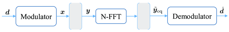
Figure 7: Complexity evaluation model.

VI-A Number of multiplications

The $N$-FFT requires $\frac{N}{2}\log_{2}(N)$ complex multiplications. The FFT-based TD-FD architecture performs $3M$ times $K$-FFT/IFFT and $3K$ times $M$-FFT/IFFT operations. Therefore, the overall transforms require $3\frac{MK}{2}\log_{2}(K)+3\frac{KM}{2}\log_{2}(M)+\frac{N}{2}\log_{2}(N)=2N\log_{2}(N)$ CMs. This is twice the number of CMs required by OFDM of length $N$. Moreover, $2N$ multiplications are needed for the product with the modulation/demodulation window. The direct modulation is achieved with $M$ times $K$-IFFT transforms using TD modulator, $K$ times $M$-IDFT with FD demodulator. Thus, $\frac{MK}{2}\log_{2}(K)+\frac{KM}{2}\log_{2}(M)+\frac{N}{2}\log_{2}(N)=N\log_{2}(N)$ CMs for the transforms. The TD direct convolution requires $MN$ and the FD requires $KN$ CMs. If only TD or FD modem is applied, two $N$-FFT/IFFT transforms with $N\log_{2}(N)$ CMs are required to transform the signal into the corresponding domain. Thus, for FFT-based TD-TD modem, we additionally need $2[\frac{MK}{2}\log_{2}(K)+2\frac{KM}{2}\log_{2}(M)+N]$, and the FFT-based FD-FD modem requires additional $2[2\frac{KM}{2}\log_{2}(M)+2\frac{MM}{2}\log_{2}(K)+N]$ CMs. On the other hand, the direct TD-TD and FD-FD require $2[\frac{MK}{2}\log_{2}(K)+MN]$, and $2[\frac{KM}{2}\log_{2}(M)+KN]$ CMs, respectively. The special case of the direct FD-FD, where the complexity can be reduced by the consideration of the sparsity of the FD prototype pulse, reduces the number of CMs for the convolution to $2LN$. This special case is useful for the processing of conventional GFDM waveform. However, the receiver pulse may overlap with more than $L$ subcarriers, e.g. when zero-forcing demodulator is applied with non-orthogonal modulation matrix.

TABLE V: Total number of CMs considering FD equalization.

Implementation method	Total number of CMs
FFT-based, TD-FD	$2N\log_{2}(N)+2N$
FFT-based, TD-TD	$2N\log_{2}(N)+N\log_{2}(M)+2N$
FFT-based, FD-FD	$2N\log_{2}(N)+N\log_{2}(K)+2N$
Direct, TD-FD	$N\log_{2}(N)+[K+M]N$
Direct, TD-TD	$N\log_{2}(N)+N\log_{2}(K)+2MN$
Direct, FD-FD	$N\log_{2}(N)+N\log_{2}(M)+2KN$
Direct ($L$ overlap), FD-FD	$N\log_{2}(N)+N\log_{2}(M)+2LN$

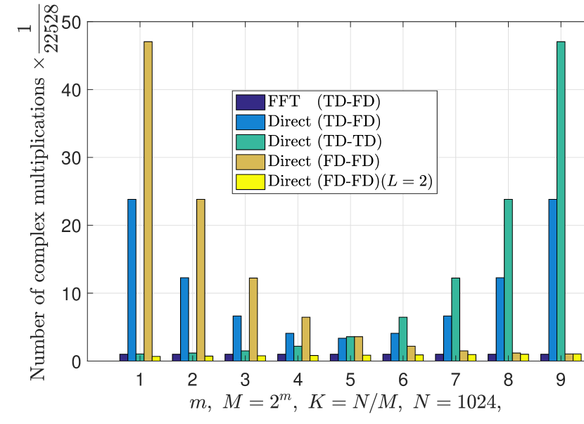
Figure 8: Number of CMs for different parameters.

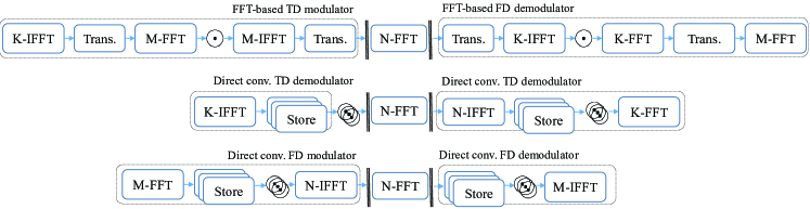
Figure 9: Efficient modem realizations.

Table V lists the overall number of CMs for the different type of modem realizations. The number of CMs required by the FFT-based TD-FD design depends only on $N=KM$ but not on the individual $K$ and $M$. The complexity is approximately $2$ times the complexity of OFDM. Obviously, the FFT based implementation should only consider the combination of TD modulation and FD demodulation to benefit from the complexity reduction. On the contrary, the complexity of the direct TD-FD implementation depends on the sum $K+M$, which in most cases requires more CMs than the one based on FD or TD only, as can be seen in Fig. 8. For $M<K$, it is more efficient to use the direct TD-TD modem, while in the case of $K<M$, using the direct FD-FD modem is more efficient. Thus, the direct convolutional structure can be switched depending on the smaller parameter. Compared with the FFT-based TD-FD, the complexity of the direct TD-TD is slightly higher with less than $2$-times up to $M<16$, $N=1024$. For $M=16$, it is $2.1$ times higher and For $K=M=32$, the complexity is $3.6$ times higher. For $M>32$, the modem can be switched to the FD-FD mode. In the special direct FD-FD with $L=2$, the complexity increases with $M$. For $M=N/4$, this modem has the same complexity as the FFT-based TD-FD, and it is about $23\%$ lower for $M=8$ and $N=1024$.

VI-B Hardware analysis

Based on the complexity analysis, we consider the most efficient setups. Namely, FFT-based TD-FD, the direct TD-TD and the direct FD-FD, as shown in Fig. 9. The architectures are compared in terms of flexibility, the required resources, and the modulation/demodulation latency, which also includes the FD equalization transform. Actually, both direct architectures are equivalent, but they differ in the placement of the $N$-IFFT block. Let $N_{\text{max}}$ be the maximum supported FFT length and $L_{\text{max}}$ the number of parallel multiplication chains in the direct modem.

VI-B1 Flexibility

The FFT-based architecture supports all combinations of radix-2 $K$ and $M$ with $KM\leq N_{\text{max}}$. The direct architecture supports all combinations that additionally satisfy $\min(K,M)\leq L_{\text{max}}$. For instance, if $N_{\text{max}}=2048$ and $L_{\text{max}}=16$, which are the typical values used in [30], then $(K,M)\in\{(32,32),(32,64),(64,32)\}$ cannot be supported. Here, it is assumed that the switching between direct TD-TD and direct FD-FD is realized. If the direct architecture is implemented with $N$-DFT IP cores instead of FFT cores, then the allowable combinations are additionally influenced by the design of the DFT core. On the other hand, the FFT-based design can provide additional flexibility by customizing the indexing of the two memories, disabling some blocks, while in the direct convolution this requires more.

VI-B2 Resource consumption

The resource consumption for real-time FPGA implementation is considered in terms of number of consumed FFT and complex multiplier IP cores, and the read-and-write (RW) and read-or-write (R/W) random-access memory (RAM) blocks. Each block RAM can fit up to $N_{\text{max}}$ complex samples. The RW-RAMs are constructed to enable read and write at the same time for the purpose of pipelining. Table VI lists the number of required resources.

TABLE VI: Number of required resources.

Implementation	FFT	Mult.	(RW)-RAM	R/W-RAM
FFT-based	$7$	$2$	$4$	$2$
Direct	$4$	$2L_{\text{max}}$	$2L_{\text{max}}$	$2L_{\text{max}}$

The FFT-based design mainly saves memory and multiplier resources. Only $2$ complex multipliers, $2$ R/W-RAM blocks are required to store the modulation/demodulation windows, and $4$ RW-RAM blocks to perform the transpose. The direct architecture consumes more complex multipliers and memory blocks depending on $L_{\text{max}}$. The FFT-based modem requires $3$ more FFT IP cores. The overall resource consumption depends on the design and implementation of the IP cores and the parallel multiplications in the direct architecture. On the other hand, the direct modem requires more resources for control and routing, which is not considered in this evaluation.

VI-B3 Latency

In this evaluation, we consider the latency of the modulation/demodulation and the FD transform at the equalizer. The latency is a measure of the delay in number of cycles between the first input data symbol at the modulator and the last output symbol at the demodulator. Considering both designs incorporate proper pipelining. Each $N$-FFT/IFFT requires $N$ cycles to load the samples and $P_{M}$ cycles to perform the transform. The memory storage of $N$ samples requires $N$ cycles, and the multiplier delay is denoted as $T_{\text{m}}$. Moreover, reading all the demodulated symbols requires $N$ cycles. From Fig. 9, it can be seen that the FFT-based implementation requires $6N$ delay cycles corresponding to $4$ memory transposes, the equalizer $N$-FFT load and the unload of the demodulated samples. Moreover, $3(M+K)$ delay cycles to load the data in $3$ time $M$-FFT/IFFT and $3$ time $K$-FFTIFFT blocks. The processing delay is $P_{N}+3(P_{K}+P_{M})+2T_{\text{m}}$ for the FFT/IFFT transforms and multipliers. The overall latency is given by

$$\small T_{\text{FFT}}=6N+3(K+M)+P_{N}+3\left(P_{K}+P_{M}\right)+2T_{\text{m}}.$$ (25)

The direct modem requires $3N$ delay cycles for intermediate storage and unloading the demodulated samples. $2N+2K$ are required for loading the samples to the FFT/IFFT blocks. The processing delay is $2P_{N}+2P_{K}+2T_{m}$ for the transforms and the parallel multipliers. Therefore, the overall delay of the direct TD-TD modem is

$$\small T_{\text{Direct-TD}}=5N+2K+2P_{N}+2P_{K}+2T_{\text{m}}.$$ (26)

Similarly for the FD-FD modem by replacing $K$ by $M$,

$$\small T_{\text{Direct-FD}}=5N+2M+2P_{N}+2P_{M}+2T_{\text{m}}.$$ (27)

The latency is influenced by the FFT size and the configuration of the FFT IP cores. The higher the FFT size, the higher the latency. It is worth mentioning that there is a trade-off between the consumed resources and latency.

Numerical example

TABLE VII: Xilinx FFT IP processing latency in cycles.

$N$	$8$	$16$	$32$	$64$	$128$	$256$	$512$	$1024$	$2048$
$P_{N}$	$57$	$110$	$126$	$177$	$241$	$387$	$643$	$1170$	$2194$

In this example, the complex multiplier has a latency $T_{m}=12$ cycles and the FFT blocks are realized based on an Xilinx-FFT IP core, which is configured in the pipelined mode with 3 complex multipliers. The processing delay of the FFT block is listed in Table VII. The difference between the FFT-based and the direct TD-TD is given by

$$\small\Delta_{\text{FFT, D-TD}}=N+K+3M+P_{K}+3P_{M}-P_{N}.$$ (28)

As shown in Fig. 10 and listed in Table VIII, the latency difference mainly depends on the size of $N$. It can be observed that the FFT-based architecture requires additional latency that decreases with the increase of $N$. For $M=16$, the additional delay decreases from $16.0\%$ at $N=256$ to $3.9\%$ at $N=2048$, and for $M=16$, it decreases from $17.7\%$ at $N=64$ to $4.3\%$ at $N=2048$. Therefore, the direct design is more appropriate for low latency requirement, especially, with smaller block length. However, this gain is at the cost of significantly increased resources consumption.

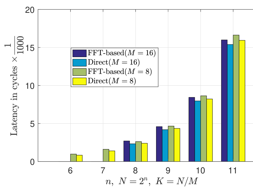
Figure 10: Latency evaluation for different parameters.

TABLE VIII: Latency evaluation.

$M=16$
$N$	-	-	$256$	$512$	$1024$	$2048$
$K$	-	-	$16$	$32$	$64$	$128$
$T_{\text{Direct-TD}}$	-	-	$2330$	$4186$	$7966$	$15390$
$\Delta_{\text{FFT, D-TD}}$	-	-	$373$	$405$	$473$	$601$
Increase $\%$	-	-	$16.0$	$9.6$	$5.9$	$3.9$
$M=8$
$N$	$64$	$128$	$256$	$512$	$1024$	$2048$
$K$	$8$	$16$	$32$	$64$	$128$	$256$
$T_{\text{Direct-TD}}$	$828$	$1398$	$2394$	$4352$	$8222$	$15938$
$\Delta_{\text{FFT, D-TD}}$	$147$	$208$	$222$	$305$	$418$	$692$
Increase $\%$	$17.7$	$14.9$	$9.3$	$7.0$	$5.0$	$4.3$

VII Conclusion

In this work, we provide an overview of multicarrier systems showing that GFDM is a main building unit for the multicarrier modulations. GFDM can be combined with multiple prototype pulses to develop and optimize new multicarrier waveforms to meet different requirements. GFDM block is represented in time and frequency domains as a superposition of parallel circular convolutions. As shown in this paper, the state of the art implementations can be represented in a unified structure that targets the realization of the convolution with parallel multiplier-memory chains. On the contrary, our proposed method realizes the convolution by means of several FFT blocks and only one multiplier. As we demonstrate in this work, the FFT-based architecture is computationally more efficient, provides more flexibility, significantly reduces the resource consumption, and maintains the latency for larger block length. Additional flexibility can be added to the FFT-based architecture with very low overhead. Namely, the customization of the indexing of the allocation memory provides a ready solution for multiuser scenarios and pilot insertion. Moreover, the bypass function allows faster processing of the classical waveforms in addition to other precoded OFDM variants. Furthermore, considering its fast run-time switching between modulation and demodulation, this architecture provides a low-cost solution for time-division duplex networks. On the other hand, the direct convolution based implementation is a convenient approach for low latency applications with short block length. However, even though the direct architectures employ parallelism, the latency reduction is marginal compared to the FFT-based architecture for larger GFDM block length. In general, the FFT-based implementation is more efficient in terms of number of complex multiplications. Nevertheless, the direct frequency-domain modem is still a reasonable choice for conventional GFDM waveform.

References

- [1] J. A. C. Bingham, “Multicarrier modulation for data transmission: an idea whose time has come,” IEEE Communications Magazine, vol. 28, no. 5, pp. 5–14, May 1990.
- [2] T. Hwang et al., “OFDM and its wireless applications: A survey,” IEEE Transactions on Vehicular Technology, vol. 58, no. 4, pp. 1673–1694, May 2009.
- [3] G. Wunder et al., “5GNOW: non-orthogonal, asynchronous waveforms for future mobile applications,” IEEE Communications Magazine, vol. 52, no. 2, pp. 97–105, February 2014.
- [4] J. van de Beek and F. Berggren, “N-continuous OFDM,” IEEE Communications Letters, vol. 13, no. 1, pp. 1–3, January 2009.
- [5] Y. Medjahdi et al., “Wola processing: A useful tool for windowed waveforms in 5G with relaxed synchronicity,” in ICC Workshops. IEEE, 2017, pp. 393–398.
- [6] T. Wild et al., “5G air interface design based on universal filtered (UF-) OFDM,” in Digital Signal Processing (DSP), 2014 19th International Conference on. IEEE, 2014, pp. 699–704.
- [7] B. Farhang-Boroujeny, “OFDM versus filter bank multicarrier,” SPM, vol. 28, no. 3, pp. 92–112, 2011.
- [8] G. Berardinelli et al., “Zero-tail DFT-spread-OFDM signals,” in 2013 IEEE Globecom Workshops (GC Wkshps), Dec 2013, pp. 229–234.
- [9] N. Michailow et al., “Generalized Frequency Division Multiplexing for 5th Generation Cellular Networks,” IEEE Trans. Commun., vol. 62, no. 9, pp. 3045–3061, Sep. 2014.
- [10] A. Nimr et al., “A study on the physical layer performance of GFDM for high throughput wireless communication,” in 2017 25th European Signal Processing Conference (EUSIPCO), Aug 2017, pp. 638–642.
- [11] G. Cherubini et al., “Filtered multitone modulation for very high-speed digital subscriber lines,” IEEE Journal on Selected Areas in Communications, vol. 20, no. 5, pp. 1016–1028, June 2002.
- [12] I. Gaspar et al., “GFDM: A Framework for Virtual PHY Services in 5G Networks,” arXiv preprint arXiv:1507.04608, 2015.
- [13] B. Farhang-Boroujeny, “OFDM versus filter bank multicarrier,” IEEE Signal Processing Magazine, vol. 28, no. 3, pp. 92–112, May 2011.
- [14] A. Fettweis, “Multidimensional wave-digital principles: from filtering to numerical integration,” in Proceedings of ICASSP ’94. IEEE International Conference on Acoustics, Speech and Signal Processing, vol. vi, April 1994, pp. VI/173–VI/181 vol.6.
- [15] J. W. Cooley and J. W. Tukey, “An algorithm for the machine calculation of complex fourier series,” Mathematics of computation, vol. 19, no. 90, pp. 297–301, 1965.
- [16] M. Matthé, L. L. Mendes, and G. Fettweis, “Generalized Frequency Division Multiplexing in a Gabor Transform Setting,” IEEE Communications Letters, vol. 18, no. 8, pp. 1379–1382, Aug 2014.
- [17] M. Danneberg et al., “Flexible GFDM implementation in FPGA with support to run-time reconfiguration,” in IEEE VTC Fall, 2015, pp. 1–2.
- [18] I. Gaspar et al., “Low complexity GFDM receiver based on sparse frequency domain processing,” in 2013 IEEE 77th Vehicular Technology Conference (VTC Spring), June 2013, pp. 1–6.
- [19] A. Nimr et al., “Optimal Radix-2 FFT Compatible Filters for GFDM,” IEEE Communications Letters, vol. 21, no. 7, pp. 1497–1500, 2017.
- [20] R. Hadani, et al., “Orthogonal time frequency space modulation,” in IEEE WCNC. IEEE, 2017, pp. 1–6.
- [21] M. Bellanger et al., “FBMC physical layer: a primer.”
- [22] I. Daubechies, et al., “Gabor time-frequency lattices and the Wexler-Raz identity,” Journal of Fourier Analysis and Applications, vol. 1, no. 4, pp. 437–478, 1994.
- [23] J. Wexler and S. Raz, “Discrete Gabor expansions,” Signal Processing, vol. 21, no. 3, pp. 207 – 220, 1990. [Online]. Available: http://www.sciencedirect.com/science/article/pii/016516849090087F
- [24] A. Janssen, “Signal analytic proofs of two basic results on lattice expansions,” Applied and Computational Harmonic Analysis, vol. 1, no. 4, pp. 350–354, 1994.
- [25] I. Gaspar et al., “Frequency-Shift Offset-QAM for GFDM,” IEEE Communications Letters, vol. 19, no. 8, pp. 1454–1457, Aug 2015.
- [26] H. Bolcskei and F. Hlawatsch, “Discrete zak transforms, polyphase transforms, and applications,” IEEE Transactions on Signal Processing, vol. 45, no. 4, pp. 851–866, April 1997.
- [27] R. M. Gray et al., “Toeplitz and circulant matrices: A review,” Foundations and Trends® in Communications and Information Theory, vol. 2, no. 3, pp. 155–239, 2006.
- [28] M. Matthé et al., “Precoded GFDM transceiver with low complexity time domain processing,” EURASIP Journal on Wireless Communications and Networking, vol. 2016, no. 1, p. 138, 2016.
- [29] A. Farhang et al., “Low complexity GFDM receiver design: A new approach,” in 2015 IEEE International Conference on Communications (ICC), London, UK, June 2015, pp. 4775–4780.
- [30] M. Danneberg et al. Flexible Transceiver Implementation. [Online]. Available: http://owl.ifn.et.tu-dresden.de/GFDM/