PUTP-2572

More Exact Results in the Wilson Loop Defect CFT: Bulk-Defect OPE,
Nonplanar Corrections and Quantum Spectral Curve

Simone Giombi***sgiombi AT princeton.edu, Shota Komatsushota.komadze AT gmail.com

Department of Physics, Princeton University, Princeton, NJ 08544, USA
School of Natural Sciences, Institute for Advanced Study, Princeton, NJ 08540, USA

Abstract

We perform exact computations of correlation functions of 1/2121/2-BPS local operators and protected operator insertions on the 1/8-BPS Wilson loop in 𝒩=4𝒩4\mathcal{N}=4 SYM. This generalizes the results of our previous paper arXiv:1802.05201, which employs supersymmetric localization, OPE and the Gram-Schmidt process. In particular, we conduct a detailed analysis for the 1/2121/2-BPS circular (or straight) Wilson loop in the planar limit, which defines an interesting nontrivial defect CFT. We compute its bulk-defect structure constants at finite ’t Hooft coupling, and present simple integral expressions in terms of the Q𝑄Q-functions that appear in the Quantum Spectral Curve—a formalism originally introduced for the computation of the operator spectrum. The results at strong coupling are found to be in precise agreement with the holographic calculation based on perturbation theory around the AdS2 string worldsheet, where they correspond to correlation functions of open string fluctuations and closed string vertex operators inserted on the worldsheet. Along the way, we clarify several aspects of the Gram-Schmidt analysis which were not addressed in the previous paper. In particular, we clarify the role played by the multi-trace operators at the non-planar level, and confirm its importance by computing the non-planar correction to the defect two-point function. We also provide a formula for the first non-planar correction to the defect correlators in terms of the Quantum Spectral Curve, which suggests the potential applicability of the formalism to the non-planar correlation functions.

1 Introduction

Wilson loops are important observables in gauge theories: They describe the coupling between a heavy probe particle and gauge fields, and are an efficient tool for distinguishing different phases of the theory. In 𝒩=4𝒩4\mathcal{N}=4 supersymmetric Yang-Mills theory, one can also consider supersymmetric generalizations of the Wilson loop which couple to the scalar field as well as to the gauge field. Such Wilson loops—in particular the 1/2-BPS Wilson loop, which preserves a maximal amount of supersymmetries—played a significant role since the early days of the AdS/CFT correspondence [1, 2]. On the gauge theory side, the exact expectation value of the 1/2121/2-BPS Wilson loop was computed first by resumming a class of ladder diagrams in [3, 4]. This computation was later justified by a rigorous argument based on supersymmetric localization in [5]. On the string theory side, the leading strong coupling behavior can be computed by evaluating the regularized area of the minimal worldsheet surface anchored on the Wilson loop at the boundary [6, 7]. The perfect matching with the strong coupling limit of the exact result [3, 4] provided one of the first important evidences for the existence of the holographic gauge/string duality. Subleading corrections at strong coupling may also be computed by evaluating the partition function for the quantum fluctuations around the classical string solution [8]. Very recently, a precise match between the localization prediction and the one-loop term on the string theory side was obtained [9].

The study of the 1/2121/2-BPS Wilson loop recently gained new interest also from the point of view of conformal defects. Indeed the 1/2121/2-BPS Wilson loop, being defined on a straight line or circular contour, preserves a SL(2,R)2𝑅(2,R) subgroup of the full conformal group [10]. Owing to this fact, it can be viewed as an example of defect conformal field theory and has been studied from various perspectives. At weak coupling, the correlation functions of insertions on the Wilson loop were computed in [11, 12], while the correlators of “defect-changing operators” which change the scalar coupling of the 1/2121/2-BPS Wilson loop were analyzed in [13]. At strong coupling, an extensive study of the correlators of the insertions was performed in [14] by using perturbation theory around the AdS2 worldsheet. Furthermore the generalization to the non-supersymmetric loop which interpolates between the 1/2121/2-BPS Wilson loop and the standard Wilson loop was explored in [15, 16, 17] both at weak and strong coupling.

In the previous paper [18], we showed that a certain class of correlators on this defect CFT111The computation in [18] applies to more general 1/8181/8-BPS Wilson loops. However, the relation to the defect CFT exists only for the 1/2121/2-BPS Wilson loop. can be computed exactly by using the combination of supersymmetric localization, OPE and the Gram-Schmidt process. The results of the computation depend nontrivially on the coupling constants and give an infinite family of defect CFT data including the structure constants of the defect BPS primaries of arbitrary lengths. Such data would provide crucial inputs for performing further analysis, for instance in the context of the conformal bootstrap [19, 20].

The results described above mostly concern the correlators of insertions inside the Wilson loop. However, from the point of view of the defect CFT, there is yet another important class of observables: the correlation functions between the “bulk” local operators defined outside the Wilson loop and the defect operators inserted on the Wilson loop. Such correlators play a central role in formulating the defect crossing equation [21, 22], and allow us to connect the defect CFT data and the CFT data in the bulk. A special example of this, which has already been studied before, is the case of correlation functions of local operators and supersymmetric Wilson loop with no insertions [6, 23, 24, 25, 26, 27]: in the defect CFT language, this gives the bulk-defect OPE coefficient of the bulk operator and the identity insertion on the defect.

The main goal of this paper is to generalize the analysis in [18] to such bulk-defect correlators: More precisely we consider the correlators of the scalar insertions Φ~Lsuperscript~Φ𝐿\tilde{\Phi}^{L} on the Wilson loop and a single-trace operator tr[Φ~J]trdelimited-[]superscript~Φ𝐽{\rm tr}[\tilde{\Phi}^{J}] defined outside the Wilson loop (the case of several bulk insertions can also be obtained from our methods). The scalar Φ~~Φ\tilde{\Phi} is a position-dependent linear combination of the scalar fields which is chosen so that the correlator becomes independent of the positions. It has another important property that the insertion of single Φ~~Φ\tilde{\Phi} is related via localization to an infinitesimal deformation of the Wilson loop. This property allows us to compute the correlators involving Φ~~Φ\tilde{\Phi}’s by the area derivatives of the expectation values of the Wilson loop, or of the correlator of the Wilson loop and the local operators, both of which are computable from localization [5, 26, 27]. As we explain in this paper, the computation can then be generalized to the correlators involving insertions of higher charges Φ~Lsuperscript~Φ𝐿\tilde{\Phi}^{L}’s (L2𝐿2L\geq 2) with the help of OPE and the Gram-Schmidt analysis.

Although the general framwork we present can be applied to the correlators at finite Ncsubscript𝑁𝑐N_{c}, in this paper we mostly focus on the leading large Ncsubscript𝑁𝑐N_{c} limit of the bulk-defect correlators. In the planar limit, we find that the results for the bulk-defect correlators can be expressed simply in terms of integrals,

𝒲[k=1nΦ~Lk]tr[Φ~J]𝑑μBJ(x)k=1nQLk(x),similar-todelimited-⟨⟩𝒲delimited-[]superscriptsubscriptproduct𝑘1𝑛superscript~Φsubscript𝐿𝑘trdelimited-[]superscript~Φ𝐽contour-integraldifferential-d𝜇subscript𝐵𝐽𝑥superscriptsubscriptproduct𝑘1𝑛subscript𝑄subscript𝐿𝑘𝑥\displaystyle\langle\mathcal{W}[\prod_{k=1}^{n}\tilde{\Phi}^{L_{k}}]{\rm tr}[\tilde{\Phi}^{J}]\rangle\sim\oint d\mu\,\,B_{J}(x)\prod_{k=1}^{n}Q_{L_{k}}(x)\,, (1.1)

where the definitions of the quantities in the formula are given in section 4.2. This formula is the generalization of the one found in our previous paper [18]. As was pointed out there, the function QL(x)subscript𝑄𝐿𝑥Q_{L}(x) that appears in the formula coincides with the so-called Q-function in the Quantum Spectral Curve formalism [28]. This appearance of the Q-function is unexpected and strongly suggests that the Quantum Spectral Curve (QSC), which was originally invented for computing the spectrum of the operators, can be useful also for analyzing the correlation functions. Using this integral representation, we expand the results at weak and strong coupling. At weak coupling, the results match the perturbative answers 𝒩=4𝒩4\mathcal{N}=4 SYM, while at strong coupling they reproduce the correlation functions of fluctuations of the string coordinates and the vertex operator on the AdS2 worldsheet, which we explicitly compute to leading order in the α1/λsimilar-tosuperscript𝛼1𝜆\alpha^{\prime}\sim 1/\sqrt{\lambda} expansion.

In the course of the computation, we also clarify several aspects of the Gram-Schmidt analysis which were not discussed in our previous paper. Most importantly we point out the necessity of including the multi-trace-like operators 𝒲[Φ~L]k=1mtr[Φ~Jk]𝒲delimited-[]superscript~Φ𝐿superscriptsubscriptproduct𝑘1𝑚trdelimited-[]superscript~Φsubscript𝐽𝑘\mathcal{W}[\tilde{\Phi}^{L}]\prod_{k=1}^{m}{\rm tr}[\tilde{\Phi}^{J_{k}}], which may be viewed from the dual perspective as bound states of open strings and closed strings, which have to be included in the defect CFT spectrum. Such operators are negligible in the planar limit but can affect the computation at the non-planar level. To confirm this effect and check the validity of our formalism, we compute the non-planar correction to the defect two-point function explicitly and check the results against the direct perturbative computations. We also provide an integral representation for the first non-planar correction in terms of the Quantum Spectral Curve (see (6.43)), which suggests the potential applicability of the QSC formalism to the nonplanar corrections.

The rest of the paper is organized as follows: In section 2, we review the definitions of the BPS Wilson loops and the results of the supersymmetric localization. After doing so, we introduce the correlators that we analyze and discuss their relations to the defect CFT data. We then explain in section 3 how to compute such correlators using OPE and the Gram-Schmidt analysis. We first present a general formalism for constructing higher-charge operators applicable to finite Ncsubscript𝑁𝑐N_{c}, and then discuss the simplification at large Ncsubscript𝑁𝑐N_{c}. Using the results in section 3, we then evaluate the bulk-defect correlators in the planar limit in section 4, deriving the integral expression and obtaining the weak- and strong-coupling expansions. These results are in perfect agreement with the direct perturbative computations at weak and strong coupling in section 5. We then discuss the non-planar corrections to the defect two-point functions in section 6. Finally in section 7 we conclude and discuss future directions. Several appendices are included to collect some explicit results of the computation.

2 Set up

Before delving into the computation, let us first explain the set up by reviewing the supersymmetric subsector of 𝒩=4𝒩4\mathcal{N}=4 SYM and showing its relation to the defect OPE data.

2.1 Supersymmetric subsector of 𝒩=4𝒩4\mathcal{N}=4 SYM

The central object in this paper is the 1/8181/8-BPS Wilson loop defined by

𝒲=1NctrPexp[C(iAj+ϵkjlxkΦl)dxj](i,j,k=1,2,3).\mathcal{W}=\frac{1}{N_{c}}{\rm tr}\,{\rm P}\exp\left[\oint_{C}\left(iA_{j}+\epsilon_{kjl}x^{k}\Phi^{l}\right)dx^{j}\right]\qquad(i,j,k=1,2,3)\,. (2.1)

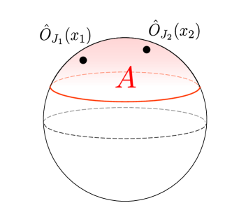
Here the Wilson loop couples to three out of the six real scalars ΦlsuperscriptΦ𝑙\Phi^{l} and the contour C𝐶C is placed on a S2superscript𝑆2S^{2} subspace of R4superscript𝑅4R^{4} (see figure 1). In the rest of this paper, we choose S2superscript𝑆2S^{2} to be of unit radius (namely x12+x22+x32=1superscriptsubscript𝑥12superscriptsubscript𝑥22superscriptsubscript𝑥321x_{1}^{2}+x_{2}^{2}+x_{3}^{2}=1) and consider only the Wilson loop in the fundamental representation. Owing to the specific choices that we made for the contour and the scalar couplings, this Wilson loop preserves four supercharges and therefore is 1/8181/8-BPS.

One can also add local operators without breaking two of the four supercharges. A prototypical example is the single-trace operator which is given by

O^J(x)𝒩J×tr[Φ~J(x)]xS2,formulae-sequencesubscript^𝑂𝐽𝑥subscript𝒩𝐽trdelimited-[]superscript~Φ𝐽𝑥𝑥superscript𝑆2\hat{O}_{J}(x)\equiv\mathcal{N}_{J}\times{\rm tr}[\tilde{\Phi}^{J}(x)]\qquad x\in S^{2}\,, (2.2)

where Φ~~Φ\tilde{\Phi} is a position-dependent linear combination of the scalar fields,

Φ~(x)=x1Φ1+x2Φ2+x3Φ3+iΦ4,~Φ𝑥subscript𝑥1superscriptΦ1subscript𝑥2superscriptΦ2subscript𝑥3superscriptΦ3𝑖superscriptΦ4\tilde{\Phi}(x)=x_{1}\Phi^{1}+x_{2}\Phi^{2}+x_{3}\Phi^{3}+i\Phi^{4}\,, (2.3)

and we chose the standard normalization for the chiral primary operators222Note that the convention here is slightly different from the one in [26, 27]: In that paper, the gauge group generators are anti-Hermitian while in this paper we stick to a more standard convention in physics in which the generators are Hermitian. This explains the extra (i)Jsuperscript𝑖𝐽(-i)^{J} factor in [26, 27]. (see [26, 27]),

𝒩J=2J/2(2π)JλJ/2J.subscript𝒩𝐽superscript2𝐽2superscript2𝜋𝐽superscript𝜆𝐽2𝐽\mathcal{N}_{J}=2^{J/2}\frac{(2\pi)^{J}}{\lambda^{J/2}\sqrt{J}}\,. (2.4)

In addition to single-trace operators, there are also multi-trace operators defined by

O^J1,,Jn(x)=k=1nO^Jk(x)xS2.formulae-sequencesubscript^𝑂subscript𝐽1subscript𝐽𝑛𝑥superscriptsubscriptproduct𝑘1𝑛subscript^𝑂subscript𝐽𝑘𝑥𝑥superscript𝑆2\hat{O}_{J_{1},\ldots,J_{n}}(x)=\prod_{k=1}^{n}\hat{O}_{J_{k}}(x)\qquad x\in S^{2}\,. (2.5)

These operators, together with the 1/8181/8-BPS Wilson loops, form a supersymmetric subsector of 𝒩=4𝒩4\mathcal{N}=4 SYM. Based on perturbation theory and AdS/CFT, it was conjectured in [29, 30] that the correlators in this subsector can be computed by the bosonic two-dimensional Yang-Mills theory on S2superscript𝑆2S^{2} (in the zero-instanton sector) with the coupling constant

g2d2=g4d22π.superscriptsubscript𝑔2d2superscriptsubscript𝑔4d22𝜋g_{\rm 2d}^{2}=-\frac{g_{\rm 4d}^{2}}{2\pi}\,. (2.6)

The relation between the observables in 2d2𝑑2d and 4d4𝑑4d is given by

𝒲trPeA2d,O^J(x)tr(i2dF2d)J.𝒲trPsuperscript𝑒contour-integralsubscript𝐴2dsubscript^𝑂𝐽𝑥trsuperscriptsubscript2d𝑖subscript𝐹2d𝐽\mathcal{W}\quad\leftrightarrow\quad{{\rm tr}}{\rm P}e^{\oint A_{\rm 2d}}\,,\qquad\hat{O}_{J}(x)\quad\leftrightarrow\quad{\rm tr}\left(i\ast_{\rm 2d}F_{\rm 2d}\right)^{J}\,. (2.7)

The conjecture was supported later by supersymmetric localization [5] and tested against a number of nontrivial checks [31, 32, 26, 27, 25, 33, 34, 35].
Refer to caption
Figure 1: Correlators of the 1/8181/8-BPS Wilson loop and local operators. The 1/8181/8-BPS Wilson loop, denoted by a red curve, can be defined on a arbitrary contour on S2superscript𝑆2S^{2} and its expectation value depends only on the area A𝐴A of the subregion inside the loop (shown as the red-shaded region). In addition to the 1/8181/8-BPS Wilson loop, one can consider the bulk single-trace operators O^Jisubscript^𝑂subscript𝐽𝑖\hat{O}_{J_{i}}. In this paper, we always assume that the bulk single-trace operators are on the same side of the Wilson loop, namely in the red-shaded region in the figure.

Thanks to its topological property, the computation in the two-dimensional Yang-Mills theory can be further reduced to simple Gaussian (multi-)matrix models [26, 27], and the results depend only on the area of the region inside the Wilson loop. For instance, the expectation value of the Wilson loop is given by

𝒲=1Z[dX]1Nctr(eX)e(4π)22A(4πA)gYM2tr(X2),delimited-⟨⟩𝒲1𝑍delimited-[]𝑑𝑋1subscript𝑁𝑐trsuperscript𝑒𝑋superscript𝑒superscript4𝜋22𝐴4𝜋𝐴superscriptsubscript𝑔YM2trsuperscript𝑋2\langle\mathcal{W}\rangle=\frac{1}{Z}\int[dX]\frac{1}{N_{c}}{\rm tr}(e^{X})e^{-\frac{(4\pi)^{2}}{2A(4\pi-A)g_{\rm YM}^{2}}{\rm tr}\left(X^{2}\right)}\,, (2.8)

where A𝐴A is the area of the subregion on S2superscript𝑆2S^{2} surrounded by the loop C𝐶C (see figure 1). Similarly the correlators of the Wilson loop and single-trace local operators are given by

𝒲O^J=delimited-⟨⟩𝒲subscript^𝑂𝐽absent\displaystyle\langle\mathcal{W}\hat{O}_{J}\rangle= 𝒩JZ[dX][dY]1Nctr(eX)tr(YJ)e(4π)22gYM2(4πA)tr(AY2+2XY),subscript𝒩𝐽𝑍delimited-[]𝑑𝑋delimited-[]𝑑𝑌1subscript𝑁𝑐trsuperscript𝑒𝑋trsuperscript𝑌𝐽superscript𝑒superscript4𝜋22superscriptsubscript𝑔YM24𝜋𝐴tr𝐴superscript𝑌22𝑋𝑌\displaystyle\frac{\mathcal{N}_{J}}{Z}\int[dX][dY]\frac{1}{N_{c}}{\rm tr}(e^{X}){\rm tr}(Y^{J})e^{-\frac{(4\pi)^{2}}{2g_{\rm YM}^{2}(4\pi-A)}{\rm tr}\left(AY^{2}+2XY\right)}\,, (2.9)
𝒲O^J1O^J2=delimited-⟨⟩𝒲subscript^𝑂subscript𝐽1subscript^𝑂subscript𝐽2absent\displaystyle\langle\mathcal{W}\hat{O}_{J_{1}}\hat{O}_{J_{2}}\rangle= 𝒩J1𝒩J2Z[dX][dY1][dY2]1Nctr(eX)tr(Y1J1)tr(Y2J2)eSWO^O^,subscript𝒩subscript𝐽1subscript𝒩subscript𝐽2𝑍delimited-[]𝑑𝑋delimited-[]𝑑subscript𝑌1delimited-[]𝑑subscript𝑌21subscript𝑁𝑐trsuperscript𝑒𝑋trsuperscriptsubscript𝑌1subscript𝐽1trsuperscriptsubscript𝑌2subscript𝐽2superscript𝑒subscript𝑆𝑊^𝑂^𝑂\displaystyle\frac{\mathcal{N}_{J_{1}}\mathcal{N}_{J_{2}}}{Z}\int[dX][dY_{1}][dY_{2}]\frac{1}{N_{c}}{\rm tr}(e^{X}){\rm tr}(Y_{1}^{J_{1}}){\rm tr}(Y_{2}^{J_{2}})e^{-S_{W\hat{O}\hat{O}}}\,,

with

SWO^O^=(4π)2(4πA)2gYM2(8πA)tr[X2(4πA)2+(Y12+Y22)8πY1Y24πA+2(Y1+Y2)X4πA].subscript𝑆𝑊^𝑂^𝑂superscript4𝜋24𝜋𝐴2superscriptsubscript𝑔YM28𝜋𝐴trdelimited-[]superscript𝑋2superscript4𝜋𝐴2superscriptsubscript𝑌12superscriptsubscript𝑌228𝜋subscript𝑌1subscript𝑌24𝜋𝐴2subscript𝑌1subscript𝑌2𝑋4𝜋𝐴S_{W\hat{O}\hat{O}}=\frac{(4\pi)^{2}(4\pi-A)}{2g_{\rm YM}^{2}(8\pi-A)}{\rm tr}\left[\frac{X^{2}}{(4\pi-A)^{2}}+(Y_{1}^{2}+Y_{2}^{2})-\frac{8\pi Y_{1}Y_{2}}{4\pi-A}+\frac{2(Y_{1}+Y_{2})X}{4\pi-A}\right]\,. (2.10)

Here we assumed that both operators are on the same side of the Wilson loop (see figure 1). These results can be straightforwardly generalized to the multi-trace operators. For instance the correlator of the Wilson loop and a double-trace operator is given by333Note that the correlator 𝒲O^J1O^J2delimited-⟨⟩𝒲subscript^𝑂subscript𝐽1subscript^𝑂subscript𝐽2\langle\mathcal{W}\hat{O}_{J_{1}}\hat{O}_{J_{2}}\rangle is different from the correlator 𝒲O^J1,J2delimited-⟨⟩𝒲subscript^𝑂subscript𝐽1subscript𝐽2\langle\mathcal{W}\hat{O}_{J_{1},J_{2}}\rangle. The former is the correlator of two single-trace operators inserted at two separate points in the bulk while the latter is the correlator of a double-trace operator inserted at a single point in the bulk. Diagrammatically, the former includes the contractions between two single-traces while the latter does not.

𝒲O^J1,J2=𝒩J1𝒩J2Z[dX][dY]1Nctr(eX)tr(YJ1)tr(YJ2)e(4π)22gYM2(4πA)tr(AY2+2XY).delimited-⟨⟩𝒲subscript^𝑂subscript𝐽1subscript𝐽2subscript𝒩subscript𝐽1subscript𝒩subscript𝐽2𝑍delimited-[]𝑑𝑋delimited-[]𝑑𝑌1subscript𝑁𝑐trsuperscript𝑒𝑋trsuperscript𝑌subscript𝐽1trsuperscript𝑌subscript𝐽2superscript𝑒superscript4𝜋22superscriptsubscript𝑔YM24𝜋𝐴tr𝐴superscript𝑌22𝑋𝑌\langle\mathcal{W}\hat{O}_{J_{1},J_{2}}\rangle=\frac{\mathcal{N}_{J_{1}}\mathcal{N}_{J_{2}}}{Z}\int[dX][dY]\frac{1}{N_{c}}{\rm tr}(e^{X}){\rm tr}(Y^{J_{1}}){\rm tr}(Y^{J_{2}})e^{-\frac{(4\pi)^{2}}{2g_{\rm YM}^{2}(4\pi-A)}{\rm tr}\left(AY^{2}+2XY\right)}\,. (2.11)

In the large Ncsubscript𝑁𝑐N_{c} limit, these correlators can be expanded in terms of the modified Bessel functions. For instance we have

𝒲=delimited-⟨⟩𝒲absent\displaystyle\langle\mathcal{W}\rangle= 2λI1(λ)+λ48Nc2I2(λ)+O(1/Nc3),2superscript𝜆subscript𝐼1superscript𝜆superscript𝜆48superscriptsubscript𝑁𝑐2subscript𝐼2superscript𝜆𝑂1superscriptsubscript𝑁𝑐3\displaystyle\frac{2}{\sqrt{\lambda^{\prime}}}I_{1}(\sqrt{\lambda^{\prime}})+\frac{\lambda^{\prime}}{48N_{c}^{2}}I_{2}(\sqrt{\lambda^{\prime}})+O(1/N_{c}^{3})\,, (2.12)
𝒲O^J=delimited-⟨⟩𝒲subscript^𝑂𝐽absent\displaystyle\langle\mathcal{W}\hat{O}_{J}\rangle= 2J/2JNc(2πa2π+a)J/2IJ(λ)+O(1/Nc2),superscript2𝐽2𝐽subscript𝑁𝑐superscript2𝜋𝑎2𝜋𝑎𝐽2subscript𝐼𝐽superscript𝜆𝑂1superscriptsubscript𝑁𝑐2\displaystyle\frac{2^{-J/2}\sqrt{J}}{N_{c}}\left(\frac{2\pi-a}{2\pi+a}\right)^{J/2}I_{J}(\sqrt{\lambda^{\prime}})+O(1/N_{c}^{2})\,,

where λsuperscript𝜆\lambda^{\prime} and a𝑎a are given by

aA2π,λλ(1a24π2),λgYM2Nc.formulae-sequence𝑎𝐴2𝜋formulae-sequencesuperscript𝜆𝜆1superscript𝑎24superscript𝜋2𝜆superscriptsubscript𝑔YM2subscript𝑁𝑐a\equiv A-2\pi\,,\qquad\lambda^{\prime}\equiv\lambda\left(1-\frac{a^{2}}{4\pi^{2}}\right)\,,\qquad\lambda\equiv g_{\rm YM}^{2}N_{c}\,. (2.13)

On the other hand, the large Ncsubscript𝑁𝑐N_{c} expansion of the correlator 𝒲O^J1O^J2delimited-⟨⟩𝒲subscript^𝑂subscript𝐽1subscript^𝑂subscript𝐽2\langle\mathcal{W}\hat{O}_{J_{1}}\hat{O}_{J_{2}}\rangle consist of two terms; the disconnected term and the connected term 𝒲O^J1O^J2=𝒲O^J1O^J2disc+𝒲O^J1O^J2conndelimited-⟨⟩𝒲subscript^𝑂subscript𝐽1subscript^𝑂subscript𝐽2subscriptdelimited-⟨⟩𝒲subscript^𝑂subscript𝐽1subscript^𝑂subscript𝐽2discsubscriptdelimited-⟨⟩𝒲subscript^𝑂subscript𝐽1subscript^𝑂subscript𝐽2conn\langle\mathcal{W}\hat{O}_{J_{1}}\hat{O}_{J_{2}}\rangle=\langle\mathcal{W}\hat{O}_{J_{1}}\hat{O}_{J_{2}}\rangle_{\rm disc}+\langle\mathcal{W}\hat{O}_{J_{1}}\hat{O}_{J_{2}}\rangle_{\rm conn}. For the purpose of this paper, we only need the disconnected term since the connected term is subleading. Written explicitly, the disconnected term is given by

𝒲O^J1O^J2disc=subscriptdelimited-⟨⟩𝒲subscript^𝑂subscript𝐽1subscript^𝑂subscript𝐽2discabsent\displaystyle\langle\mathcal{W}\hat{O}_{J_{1}}\hat{O}_{J_{2}}\rangle_{\rm disc}= (12)J1δJ1,J2𝒲superscript12subscript𝐽1subscript𝛿subscript𝐽1subscript𝐽2delimited-⟨⟩𝒲\displaystyle\left(-\frac{1}{2}\right)^{J_{1}}\delta_{J_{1},J_{2}}\langle\mathcal{W}\rangle (2.14)
=(12)J1δJ1,J2[2λI1(λ)+λ48Nc2I2(λ)+O(1/Nc3)].absentsuperscript12subscript𝐽1subscript𝛿subscript𝐽1subscript𝐽2delimited-[]2superscript𝜆subscript𝐼1superscript𝜆superscript𝜆48superscriptsubscript𝑁𝑐2subscript𝐼2superscript𝜆𝑂1superscriptsubscript𝑁𝑐3\displaystyle=\left(-\frac{1}{2}\right)^{J_{1}}\delta_{J_{1},J_{2}}\left[\frac{2}{\sqrt{\lambda^{\prime}}}I_{1}(\sqrt{\lambda^{\prime}})+\frac{\lambda^{\prime}}{48N_{c}^{2}}I_{2}(\sqrt{\lambda^{\prime}})+O(1/N_{c}^{3})\right]\,.

The explicit expression for the connected term can be found in Appendix A.

2.2 Operators on the Wilson loop and the area derivatives

In addition to the operators discussed in the previous subsection whose correlators can be computed by localization rather directly, there is another interesting class of operators which are obtained by inserting scalars inside a Wilson loop trace:

𝒲[:Φ~L1::Φ~L2::Φ~Ln:]1NctrP[:Φ~L1(τ1)::Φ~Ln(τn):eC(iAj+ϵkjlxkΦl)𝑑xj].\mathcal{W}[:\!\tilde{\Phi}^{L_{1}}\!:\,:\!\tilde{\Phi}^{L_{2}}\!:\,\cdots:\!\tilde{\Phi}^{L_{n}}\!:\,]\equiv\frac{1}{N_{c}}{\rm tr}{\rm P}\left[:\!\tilde{\Phi}^{L_{1}}(\tau_{1})\!:\,\cdots:\!\tilde{\Phi}^{L_{n}}(\tau_{n})\!:\,e^{\oint_{C}\left(iA_{j}+\epsilon_{kjl}x^{k}\Phi^{l}\right)dx^{j}}\right]\,. (2.15)

Here we parametrize the loop by τ[0,2π]𝜏02𝜋\tau\in[0,2\pi]. Note also that we put a normal-ordering symbol to Φ~Lsuperscript~Φ𝐿\tilde{\Phi}^{L} in order to emphasize the absence of self-contractions inside each operator. At this point this may seem unnecessary complication, but the reason for doing this will become clear in the next section.

As shown in [5], the insertion of a single scalar corresponds to the insertion of a dual field strength of the two-dimensional Yang-Mills theory,

Φ~iF2d,~Φ𝑖subscript𝐹2d\tilde{\Phi}\quad\leftrightarrow\quad i\ast F_{\rm 2d}\,, (2.16)

which in turn is related to a small deformation of the (2d) Wilson loop. This correspondence allows us to relate the correlators of multiple Φ~~Φ\tilde{\Phi}’s to the area derivatives of the Wilson loop expectation value444Owing to the relation to the 2d Yang-Mills theory, these correlators are also independent of the postions (namely τksubscript𝜏𝑘\tau_{k}’s).,

𝒲[Φ~Φ~n]=n𝒲(A)n.delimited-⟨⟩𝒲delimited-[]subscript~Φ~Φ𝑛superscript𝑛delimited-⟨⟩𝒲superscript𝐴𝑛\langle\mathcal{W}[\,\underbracket{\tilde{\Phi}\cdots\tilde{\Phi}}_{n}\,]\rangle=\frac{\partial^{n}\langle\mathcal{W}\rangle}{(\partial A)^{n}}\,. (2.17)

As discussed in the previous work [18], it is also possible to relate the insertion of higher-charge operators 𝒲[:Φ~L:]\mathcal{W}[:\!\tilde{\Phi}^{L}\!:\,] to the area derivatives. This however requires the use of the Gram-Schmidt orthogonalization, which we will review and refine in the next section, and the results in general take a more complicated form (although they can computed systematically from the localization results).

Now, putting together these operator insertions with the operators discussed in the previous subsection, one can consider a variety of correlators of the form,

GL1,,Ln|J1,,Jm𝒲[k=1n:Φ~Lk:]k=1mO^Jk.\displaystyle G_{L_{1},\ldots,L_{n}|J_{1},\ldots,J_{m}}\equiv\langle\mathcal{W}[\prod_{k=1}^{n}:\!\tilde{\Phi}^{L_{k}}\!:\,]\prod_{k=1}^{m}\hat{O}_{J_{k}}\rangle\,. (2.18)

In what follows, we call these correlators topological correlators since they do not depend on the positions. The main goal of this paper is to analyze these correlators555Although we mostly focus on the simplest correlators 𝒲[:Φ~L:]O^J\langle\mathcal{W}[:\!\tilde{\Phi}^{L}\!:\,]\hat{O}_{J}\rangle in this paper, the general methodology that we develop is applicable also to more complicated correlators (2.18). by generalizing the arguments in [18].

2.3 Relation to the defect CFT data

When the contour is a circle along the equator of S2superscript𝑆2S^{2}, the Wilson loop preserves higher amount of supersymmetries and becomes 1/2121/2-BPS:

𝒲1/2BPS=1NctrPexp[equator(iAjx˙j+Φ3|x˙|)𝑑τ].subscript𝒲12BPS1subscript𝑁𝑐trPsubscriptcontour-integralequator𝑖subscript𝐴𝑗superscript˙𝑥𝑗superscriptΦ3˙𝑥differential-d𝜏\mathcal{W}_{{\rm 1/2-BPS}}=\frac{1}{N_{c}}{\rm tr}{\rm P}\exp\left[\oint_{{\rm equator}}\left(iA_{j}\dot{x}^{j}+\Phi^{3}|\dot{x}|\right)d\tau\right]\,. (2.19)

An important feature of this Wilson loop is that it preserves the SL(2,R) conformal symmetry666The full symmetry group preserved by the circular Wilson loop is OSP(4|4)conditionalsuperscript44(4^{\ast}|4). and therefore can be regarded as a conformal defect. This in particular implies that one can extract the defect CFT data from the correlators in the supersymmetric subsector.

Before discussing how to do so, let us first introduce the normalized correlators, defined by

𝒲[]𝒲[]𝒲,delimited-⟨⟩delimited-⟨⟩𝒲delimited-[]delimited-⟨⟩𝒲delimited-[]delimited-⟨⟩𝒲\langle\!\langle\mathcal{W}[\cdots]\cdots\rangle\!\rangle\equiv\frac{\langle\mathcal{W}[\cdots]\cdots\rangle}{\langle\mathcal{W}\rangle}\,, (2.20)

where \cdots denote either the operators on the Wilson loop or the operators in the bulk depending on whether it is inside 𝒲[]𝒲\mathcal{W}[\,\,\,\,] or not. Taking such a ratio renders the expectation value of the identity operator to be unity and make the correlators obey the standard defect CFT axioms. We then consider the following correlators of the protected operators,

𝒢L1,L2subscript𝒢subscript𝐿1subscript𝐿2\displaystyle\mathcal{G}_{L_{1},L_{2}} 𝒲[(u1Φ)L1(τ1)(u2Φ)L2(τ2)]circle,absentsubscriptdelimited-⟨⟩delimited-⟨⟩𝒲delimited-[]superscriptsubscript𝑢1Φsubscript𝐿1subscript𝜏1superscriptsubscript𝑢2Φsubscript𝐿2subscript𝜏2circle\displaystyle\equiv\langle\!\langle\mathcal{W}[(u_{1}\cdot\vec{\Phi})^{L_{1}}(\tau_{1})(u_{2}\cdot\vec{\Phi})^{L_{2}}(\tau_{2})]\rangle\!\rangle_{\rm circle}\,, (2.21)
𝒢L1,L2,L3subscript𝒢subscript𝐿1subscript𝐿2subscript𝐿3\displaystyle\mathcal{G}_{L_{1},L_{2},L_{3}} 𝒲[(u1Φ)L1(τ1)(u2Φ)L2(τ2)(u3Φ)L3(τ3)]circle,absentsubscriptdelimited-⟨⟩delimited-⟨⟩𝒲delimited-[]superscriptsubscript𝑢1Φsubscript𝐿1subscript𝜏1superscriptsubscript𝑢2Φsubscript𝐿2subscript𝜏2superscriptsubscript𝑢3Φsubscript𝐿3subscript𝜏3circle\displaystyle\equiv\langle\!\langle\mathcal{W}[(u_{1}\cdot\vec{\Phi})^{L_{1}}(\tau_{1})(u_{2}\cdot\vec{\Phi})^{L_{2}}(\tau_{2})(u_{3}\cdot\vec{\Phi})^{L_{3}}(\tau_{3})]\rangle\!\rangle_{\rm circle}\,,
𝒢L|Jsubscript𝒢conditional𝐿𝐽\displaystyle\mathcal{G}_{L|J} 𝒲[(uΦ)L(τ)]tr(UΦ)J(x)circle.absentsubscriptdelimited-⟨⟩delimited-⟨⟩𝒲delimited-[]superscript𝑢Φ𝐿𝜏trsuperscript𝑈Φ𝐽superscript𝑥circle\displaystyle\equiv\langle\!\langle\mathcal{W}[(u\cdot\vec{\Phi})^{L}(\tau)]\,\,{\rm tr}(U\cdot\vec{\Phi})^{J}(x^{\prime})\rangle\!\rangle_{\rm circle}\,.

Here Φ=(Φ1,Φ2,Φ3,Φ4,Φ5,Φ6)ΦsubscriptΦ1subscriptΦ2subscriptΦ3subscriptΦ4subscriptΦ5subscriptΦ6\vec{\Phi}=\left(\Phi_{1},\Phi_{2},\Phi_{3},\Phi_{4},\Phi_{5},\Phi_{6}\right) and U𝑈U’s and u𝑢u’s are six-dimensional null vectors satisfying UU=uu=0𝑈𝑈𝑢𝑢0U\cdot U=u\cdot u=0. In addition, we require the third components of u𝑢u’s to vanish in order to make the operators (ukΦ)Lksuperscriptsubscript𝑢𝑘Φsubscript𝐿𝑘(u_{k}\cdot\vec{\Phi})^{L_{k}} to have protected conformal dimensions (in other words, the null vector u𝑢u projects onto a symmetric traceless representation of the SO(5)SO(6)𝑆𝑂5𝑆𝑂6SO(5)\subset SO(6) preserved by the 1/2-BPS Wilson loop). Unlike the correlators in the supersymmetric subsector that we discussed in the previous subsections, these correlators depend on the positions of the operators. However, thanks to the conformal symmetry and the R-symmetry, the position dependence can be completely fixed to be

𝒢L1,L2subscript𝒢subscript𝐿1subscript𝐿2\displaystyle\mathcal{G}_{L_{1},L_{2}} =nL1×δL1,L2(u1u2)L1(2sinτ122)2L1,absentsubscript𝑛subscript𝐿1subscript𝛿subscript𝐿1subscript𝐿2superscriptsubscript𝑢1subscript𝑢2subscript𝐿1superscript2subscript𝜏1222subscript𝐿1\displaystyle=n_{L_{1}}\times\frac{\delta_{L_{1},L_{2}}(u_{1}\cdot u_{2})^{L_{1}}}{(2\sin\frac{\tau_{12}}{2})^{2L_{1}}}\,, (2.22)
𝒢L1,L2,L3subscript𝒢subscript𝐿1subscript𝐿2subscript𝐿3\displaystyle\mathcal{G}_{L_{1},L_{2},L_{3}} =cL1,L2,L3×(u1u2)L12|3(u2u3)L23|1(u3u1)L31|2(2sinτ122)2L12|3(2sinτ232)2L23|1(2sinτ312)2L31|2,absentsubscript𝑐subscript𝐿1subscript𝐿2subscript𝐿3superscriptsubscript𝑢1subscript𝑢2subscript𝐿conditional123superscriptsubscript𝑢2subscript𝑢3subscript𝐿conditional231superscriptsubscript𝑢3subscript𝑢1subscript𝐿conditional312superscript2subscript𝜏1222subscript𝐿conditional123superscript2subscript𝜏2322subscript𝐿conditional231superscript2subscript𝜏3122subscript𝐿conditional312\displaystyle=c_{L_{1},L_{2},L_{3}}\times\frac{(u_{1}\cdot u_{2})^{L_{12|3}}(u_{2}\cdot u_{3})^{L_{23|1}}(u_{3}\cdot u_{1})^{L_{31|2}}}{(2\sin\frac{\tau_{12}}{2})^{2L_{12|3}}(2\sin\frac{\tau_{23}}{2})^{2L_{23|1}}(2\sin\frac{\tau_{31}}{2})^{2L_{31|2}}}\,,
𝒢L|Jsubscript𝒢conditional𝐿𝐽\displaystyle\mathcal{G}_{L|J} =cL|J×(uU)L(U3)JL|xx(τ)|2L|x|JL,absentsubscript𝑐conditional𝐿𝐽superscript𝑢𝑈𝐿superscriptsubscript𝑈3𝐽𝐿superscriptsuperscript𝑥𝑥𝜏2𝐿superscriptsubscriptsuperscript𝑥perpendicular-to𝐽𝐿\displaystyle=c_{L|J}\times\frac{(u\cdot U)^{L}(U_{3})^{J-L}}{|x^{\prime}-x(\tau)|^{2L}|x^{\prime}_{\perp}|^{J-L}}\,,

where τijτiτjsubscript𝜏𝑖𝑗subscript𝜏𝑖subscript𝜏𝑗\tau_{ij}\equiv\tau_{i}-\tau_{j}, Lij|k(Li+LjLk)/2subscript𝐿conditional𝑖𝑗𝑘subscript𝐿𝑖subscript𝐿𝑗subscript𝐿𝑘2L_{ij|k}\equiv(L_{i}+L_{j}-L_{k})/2 and |x|subscriptsuperscript𝑥perpendicular-to|x^{\prime}_{\perp}| is given by

|x|=[1+(x1)2+(x2)2+(x3)2+(x4)2]24[(x1)2+(x2)2]2.subscriptsuperscript𝑥perpendicular-tosuperscriptdelimited-[]1superscriptsuperscriptsubscript𝑥12superscriptsuperscriptsubscript𝑥22superscriptsuperscriptsubscript𝑥32superscriptsuperscriptsubscript𝑥4224delimited-[]superscriptsuperscriptsubscript𝑥12superscriptsuperscriptsubscript𝑥222|x^{\prime}_{\perp}|=\frac{\sqrt{\left[1+(x_{1}^{\prime})^{2}+(x_{2}^{\prime})^{2}+(x_{3}^{\prime})^{2}+(x_{4}^{\prime})^{2}\right]^{2}-4\left[(x_{1}^{\prime})^{2}+(x_{2}^{\prime})^{2}\right]}}{2}\,. (2.23)

The constants nL1subscript𝑛subscript𝐿1n_{L_{1}}, CL1,L2,L3subscript𝐶subscript𝐿1subscript𝐿2subscript𝐿3C_{L_{1},L_{2},L_{3}} and cL|Jsubscript𝑐conditional𝐿𝐽c_{L|J} are the defect CFT data which are nontrivial functions of the ’t Hooft coupling and the rank of the gauge group. One can also perform the conformal transformation to map the Wilson loop to a straight line. In that case, one simply needs to perform the following replacement for 𝒢L1,L2subscript𝒢subscript𝐿1subscript𝐿2\mathcal{G}_{L_{1},L_{2}} and 𝒢L1,L2,L3subscript𝒢subscript𝐿1subscript𝐿2subscript𝐿3\mathcal{G}_{L_{1},L_{2},L_{3}},

2sinτij2|x(τi)x(τj)|,2subscript𝜏𝑖𝑗2maps-to𝑥subscript𝜏𝑖𝑥subscript𝜏𝑗2\sin\frac{\tau_{ij}}{2}\quad\mapsto\quad|x(\tau_{i})-x(\tau_{j})|\,, (2.24)

while the expression for 𝒢L|Jsubscript𝒢conditional𝐿𝐽\mathcal{G}_{L|J} still applies if we interpret |x|superscriptsubscript𝑥perpendicular-to|x_{\perp}^{\prime}| as the distance in the direction perpendicular to the Wilson loop.

These correlators reduce to the topological correlators (2.18) upon the following specification of the parameters

ui=(cosτi,sinτi,0,i,0,0),U=(x1,x2,x3,i,0,0),xS2.formulae-sequencesubscript𝑢𝑖subscript𝜏𝑖subscript𝜏𝑖0𝑖00formulae-sequence𝑈subscriptsuperscript𝑥1subscriptsuperscript𝑥2subscriptsuperscript𝑥3𝑖00superscript𝑥superscript𝑆2\displaystyle u_{i}=(\cos\tau_{i},\sin\tau_{i},0,i,0,0)\,,\qquad U=(x^{\prime}_{1},x^{\prime}_{2},x^{\prime}_{3},i,0,0)\,,\qquad x^{\prime}\in S^{2}\,. (2.25)

The results read

GL1,L2𝒲subscript𝐺subscript𝐿1subscript𝐿2delimited-⟨⟩𝒲\displaystyle\frac{G_{L_{1},L_{2}}}{\langle\mathcal{W}\rangle} =(12)L1×δL1,L2nL1,GL1,L2,L3𝒲=(12)L1+L2+L32×cL1,L2,L3,formulae-sequenceabsentsuperscript12subscript𝐿1subscript𝛿subscript𝐿1subscript𝐿2subscript𝑛subscript𝐿1subscript𝐺subscript𝐿1subscript𝐿2subscript𝐿3delimited-⟨⟩𝒲superscript12subscript𝐿1subscript𝐿2subscript𝐿32subscript𝑐subscript𝐿1subscript𝐿2subscript𝐿3\displaystyle=\left(-\frac{1}{2}\right)^{L_{1}}\times\delta_{L_{1},L_{2}}n_{L_{1}}\,,\qquad\frac{G_{L_{1},L_{2},L_{3}}}{\langle\mathcal{W}\rangle}=\left(-\frac{1}{2}\right)^{\frac{L_{1}+L_{2}+L_{3}}{2}}\times c_{L_{1},L_{2},L_{3}}\,, (2.26)
GL|J𝒲subscript𝐺conditional𝐿𝐽delimited-⟨⟩𝒲\displaystyle\frac{G_{L|J}}{\langle\mathcal{W}\rangle} =(12)L×cL|J.absentsuperscript12𝐿subscript𝑐conditional𝐿𝐽\displaystyle=\left(-\frac{1}{2}\right)^{L}\times c_{L|J}\,.

This shows that the topological correlators coincide with the defect CFT data up to trivial overall factors.

It is sometimes useful to unit-normalize the two-point functions on the Wilson loop. In such normalization, the structure constants are given as follows:

CL1,L2,L3cL1,L2,L3nL1nL2nL3,CL|JcL|JnL.formulae-sequencesubscript𝐶subscript𝐿1subscript𝐿2subscript𝐿3subscript𝑐subscript𝐿1subscript𝐿2subscript𝐿3subscript𝑛subscript𝐿1subscript𝑛subscript𝐿2subscript𝑛subscript𝐿3subscript𝐶conditional𝐿𝐽subscript𝑐conditional𝐿𝐽subscript𝑛𝐿\displaystyle C_{L_{1},L_{2},L_{3}}\equiv\frac{c_{L_{1},L_{2},L_{3}}}{\sqrt{n_{L_{1}}n_{L_{2}}n_{L_{3}}}}\,,\qquad C_{L|J}\equiv\frac{c_{L|J}}{\sqrt{n_{L}}}\,. (2.27)

3 Construction of higher-charge operators

In this section, we construct general operator insertions :Φ~L::\!\tilde{\Phi}^{L}\!:\, on the Wilson loop in the supersymmetric subsector using the OPE and the Gram-Schmidt process. The same idea was employed already in the previous work [18], but here we elucidate several important points which were not accounted for in [18]. Although they are largely negligible at large Ncsubscript𝑁𝑐N_{c}, they have important consequences on the bulk-defect correlators and the non-planar corrections, as will be shown in sections 4 and 6.

3.1 Basic idea

Before presenting a general construction, let us explain the basic idea of our approach using simple examples of correlators on the 1/2121/2-BPS circular loop. Along the way we clarify three important aspects (bound state, degeneracy and mixing with multi-trace operators) which were not discussed in our previous construction [18].

The basic strategy is to construct complicated operators from simpler operators using the OPE. The simplest operator (apart from the identity) on the 1/2121/2-BPS Wilson loop is the single-scalar insertion 𝒲[:Φ~:]\mathcal{W}[:\!\tilde{\Phi}\!:\,]. As discussed above, the correlator of this operator can be computed directly by taking area derivatives of the localization result.

Bound state

In addition to 𝒲[:Φ~:]\mathcal{W}[:\!\tilde{\Phi}\!:\,], there is yet another operator on the Wilson loop with the same R𝑅R-charge, :𝒲tr[Φ~]::\!\mathcal{W}\,{\rm tr}[\tilde{\Phi}]\!:\,,777In this paper we take the gauge group to be U(N)𝑈𝑁U(N) for simplicity. In the case of SU(N)𝑆𝑈𝑁SU(N), this type of operator would appear first at charge 2, i.e. :𝒲tr[Φ~2]::\!\mathcal{W}\,{\rm tr}[\tilde{\Phi}^{2}]\!:\,. namely a single-trace operator placed at a point on the Wilson loop. On the string-theory side, this operator, and its higher charge generalizations, correspond to a bound state of open and closed strings. Although it might not be so obvious why it must be included in the defect CFT spectrum, one can show that such operators are necessary for the consistency of the bulk-defect crossing equation as explained in Appendix A. Unlike the insertion 𝒲[:Φ~:]\mathcal{W}[:\!\tilde{\Phi}\!:\,], this operator is not related to the area derivatives of the Wilson loop expectation value. To construct this operator, we instead need to consider a correlator of the Wilson loop and a bulk single-trace operator. Since the correlator is independent of the positions, we can bring the bulk operator arbitrarily close to a point on the loop without affecting its expectation value. After doing so, we perform the bulk-defect OPE to get

tr[Φ~]|bulk𝒲=bulk-defect OPE:𝒲tr[Φ~]:+c0𝒲.\left.{\rm tr}[\tilde{\Phi}]\right|_{\rm bulk}\mathcal{W}\quad\overset{\text{bulk-defect OPE}}{=}\quad:\!\mathcal{W}\,{\rm tr}[\tilde{\Phi}]\!:\,+c_{0}\mathcal{W}\,. (3.1)

As shown above, in addition to :𝒲tr[Φ~]::\!\mathcal{W}\,{\rm tr}[\tilde{\Phi}]\!:\,, this process produces another operator, which is the identity operator on the Wilson loop (or, equivalently, the Wilson loop itself). The coefficient c0subscript𝑐0c_{0} then corresponds to the bulk-defect structure constant between tr[Φ~]trdelimited-[]~Φ{\rm tr}[\tilde{\Phi}] in the bulk and the identity operator on the Wilson loop, and is given by the expectation value

c0=𝒲[𝟏]tr[Φ~](𝒲tr[Φ~]/𝒲).subscript𝑐0annotateddelimited-⟨⟩delimited-⟨⟩𝒲delimited-[]1trdelimited-[]~Φabsentdelimited-⟨⟩𝒲trdelimited-[]~Φdelimited-⟨⟩𝒲c_{0}=\langle\!\langle\mathcal{W}[{\bf 1}]\,{\rm tr}[\tilde{\Phi}]\rangle\!\rangle\quad\left(\equiv\langle\mathcal{W}\,{\rm tr}[\tilde{\Phi}]\rangle/\langle\mathcal{W}\rangle\right)\,. (3.2)

Inverting the relation (3.1), we obtain

:𝒲tr[Φ~]:=tr[Φ~]|bulk𝒲c0𝒲.:\!\mathcal{W}\,{\rm tr}[\tilde{\Phi}]\!:\,=\left.{\rm tr}[\tilde{\Phi}]\right|_{\rm bulk}\mathcal{W}-c_{0}\mathcal{W}\,. (3.3)

This expression allows us to relate the correlators of :𝒲tr[Φ~]::\!\mathcal{W}\,{\rm tr}[\tilde{\Phi}]\!:\, to the correlators that are computable from supersymmetric localization.

Degeneracy and orthogonalization

Let us next consider the length-2 operators. In general, there are four different length-2 operators,

𝒲[:Φ~2:],:𝒲[Φ~]tr[Φ]:,:𝒲tr[Φ~2]:,:𝒲(tr[Φ~])2:.\mathcal{W}[:\!\tilde{\Phi}^{2}\!:\,]\,,\qquad:\!\mathcal{W}[\tilde{\Phi}]{\rm tr}[\Phi]\!:\,\,,\qquad:\!\mathcal{W}{\rm tr}[\tilde{\Phi}^{2}]\!:\,\,,\qquad:\!\mathcal{W}({\rm tr}[\tilde{\Phi}])^{2}\!:\,\,. (3.4)

Among these four operators, the first operator 𝒲[:Φ~2:]\mathcal{W}[:\!\tilde{\Phi}^{2}\!:\,] can be constructed by taking the defect OPE of two scalar insertions,

𝒲[Φ~Φ~]=defect OPE𝒲[:Φ~2:]+c1𝒲,\mathcal{W}[\tilde{\Phi}\tilde{\Phi}]\qquad\overset{\text{defect OPE}}{=}\qquad\mathcal{W}[:\!\tilde{\Phi}^{2}\!:\,]+c_{1}\mathcal{W}\,, (3.5)

where the second term on the right hand side comes from the self-contraction of the two scalars and c1subscript𝑐1c_{1} is the defect structure constant of two Φ~~Φ\tilde{\Phi}’s and the identity operator,

c1=𝒲[Φ~Φ~𝟏](𝒲[Φ~Φ~]/𝒲).subscript𝑐1annotateddelimited-⟨⟩delimited-⟨⟩𝒲delimited-[]~Φ~Φ1absentdelimited-⟨⟩𝒲delimited-[]~Φ~Φdelimited-⟨⟩𝒲c_{1}=\langle\!\langle\mathcal{W}[\tilde{\Phi}\tilde{\Phi}{\bf 1}]\rangle\!\rangle\left(\equiv\langle\mathcal{W}[\tilde{\Phi}\tilde{\Phi}]\rangle/\langle\mathcal{W}\rangle\right)\,. (3.6)

Then by subtracting this extra contribution, we can single out 𝒲[:Φ~2:]\mathcal{W}[:\!\tilde{\Phi}^{2}\!:\,]. To compute other operators, we need to consider bulk-defect correlators as was the case for the operator 𝒲[:Φ~:]\mathcal{W}[:\!\tilde{\Phi}\!:\,]. For instance, the second operator :𝒲[Φ~]tr[Φ]::\!\mathcal{W}[\tilde{\Phi}]{\rm tr}[\Phi]\!:\, can be obtained by taking the combination of the defect OPE and the bulk-defect OPE of tr[Φ~]trdelimited-[]~Φ{\rm tr}[\tilde{\Phi}] in the bulk and 𝒲[Φ~]𝒲delimited-[]~Φ\mathcal{W}[\tilde{\Phi}], namely

tr[Φ~]|bulk𝒲[Φ~]=OPE:𝒲[Φ~]tr[Φ]:+c2𝒲[:Φ~:]+c3𝒲.\left.{\rm tr}[\tilde{\Phi}]\right|_{\rm bulk}\mathcal{W}[\tilde{\Phi}]\qquad\overset{\rm OPE}{=}\qquad:\!\mathcal{W}[\tilde{\Phi}]{\rm tr}[\Phi]\!:\,+c_{2}\mathcal{W}[:\!\tilde{\Phi}\!:\,]+c_{3}\mathcal{W}\,. (3.7)

Here the second term comes from the contraction of the bulk tr[Φ~]trdelimited-[]~Φ{\rm tr}[\tilde{\Phi}] with the Wilson loop while the last term comes from the contraction of tr[Φ~]trdelimited-[]~Φ{\rm tr}[\tilde{\Phi}] and the insertion on the loop Φ~~Φ\tilde{\Phi}. The OPE coefficients c2subscript𝑐2c_{2} and c3subscript𝑐3c_{3} are given by888Note that, for c2subscript𝑐2c_{2}, one needs to divide by the norm of the resulting state 𝒲[Φ~]𝒲delimited-[]~Φ\mathcal{W}[\tilde{\Phi}] in order to have the correct OPE expansion.

c2=𝒲[Φ~Φ~]tr[Φ~]𝒲[Φ~Φ~],subscript𝑐2delimited-⟨⟩delimited-⟨⟩𝒲delimited-[]~Φ~Φtrdelimited-[]~Φdelimited-⟨⟩delimited-⟨⟩𝒲delimited-[]~Φ~Φ\displaystyle c_{2}=\frac{\langle\!\langle\mathcal{W}[\tilde{\Phi}\tilde{\Phi}]{\rm tr}[\tilde{\Phi}]\rangle\!\rangle}{\langle\!\langle\mathcal{W}[\tilde{\Phi}\tilde{\Phi}]\rangle\!\rangle}\,,\qquad c3=𝒲[Φ~]tr[Φ~].subscript𝑐3delimited-⟨⟩delimited-⟨⟩𝒲delimited-[]~Φtrdelimited-[]~Φ\displaystyle c_{3}=\langle\!\langle\mathcal{W}[\tilde{\Phi}]{\rm tr}[\tilde{\Phi}]\rangle\!\rangle\,. (3.8)

Repeating the same procedures for the other two operators, one can define sets of normal-ordered operators. The resulting operators are free of admixiture of operators with different R𝑅R-charges and they are all equally good defect primaries. However, they have one unsatisfactory feature that they are not necessarily orthogonal to each other; namely the two-point functions of different operators do not vanish in general. To make them orthogonal to each other, one has to take appropriate linear combinations of these four operators. The choice of the linear combinations is not unique since all these operator have the same quantum number and physically indistinguishable especially at finite Ncsubscript𝑁𝑐N_{c}, where the distinction by the number of traces becomes obscured. In this paper, we make a choice that is most suited for studying the correlators at large Ncsubscript𝑁𝑐N_{c}; namely we define 𝒲[:Φ~k:]\mathcal{W}[:\!\tilde{\Phi}^{k}\!:\,] without performing further subtraction while for the rest of the operators we take appropriate linear combinations so that they become orthogonal to each other and also to 𝒲[:Φ~k:]\mathcal{W}[:\!\tilde{\Phi}^{k}\!:\,].

Mixing with “multi-trace” operators

In the examples discussed so far, the self-contraction of insertions on the Wilson loop 𝒲[Φ~Φ~]𝒲delimited-[]~Φ~Φ\mathcal{W}[\tilde{\Phi}\cdots\tilde{\Phi}] only produced the operators of the same kind, 𝒲[Φ~Φ~]𝒲delimited-[]~Φ~Φ\mathcal{W}[\tilde{\Phi}\cdots\tilde{\Phi}]. However, starting from length-333 operators, a new effect shows up which inevitably mixes the operators of different types, namely the operators involving multi-traces999We call these operators multi-trace operators since the Wilson loop itself already contains a trace. e.g. 𝒲[Φ~Φ~]tr[Φ~J]𝒲delimited-[]~Φ~Φtrdelimited-[]superscript~Φ𝐽\mathcal{W}[\tilde{\Phi}\cdots\tilde{\Phi}]{\rm tr}[\tilde{\Phi}^{J}].

Refer to caption

(a)

Refer to caption

(b)

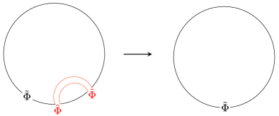
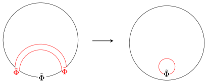
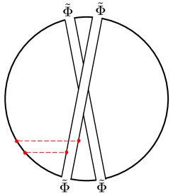
Figure 2: Wick contractions of the insertions on the Wilson loop. (a) In the planar limit, the Wick contractions (denoted by red double lines) can only connect neighboring insertions. Therefore, the resulting operator is again an insertion on the Wilson loop. (b) On the other hand, at the non-planar level, one can connect non-neighboring insertions by a propagator. This produces a closed index loop for the remaining fields and converts them into a single-trace operator. It is therefore necessary to include the “multi-trace” operators in the spectrum on the Wilson loop.

To see this explicitly, let us consider the OPE of three Φ~~Φ\tilde{\Phi}’s inserted on the Wilson loop. At weak coupling, the OPE simply amounts to performing the Wick contractions. At large Ncsubscript𝑁𝑐N_{c}, due to planarity, the only allowed contraction is to connect two neighboring Φ~~Φ\tilde{\Phi}’s as shown in figure 2-(a). As shown in the figure, we then get a single insertion Φ~~Φ\tilde{\Phi} on the Wilson loop, namely 𝒲[Φ~]𝒲delimited-[]~Φ\mathcal{W}[\tilde{\Phi}]. However, at the non-planar level, we can Wick-contract non-neighboring Φ~~Φ\tilde{\Phi}’s as shown in figure 2-(b). This produces a closed color-index loop for the remaining Φ~~Φ\tilde{\Phi} in the middle, and converts it into a single-trace operator tr[Φ~]trdelimited-[]~Φ{\rm tr}[\tilde{\Phi}]. Thus the OPE of three Φ~~Φ\tilde{\Phi}’s takes the following form:

𝒲[Φ~Φ~Φ~]=𝒲[:Φ~3:]+c4𝒲[:Φ~:]+c5𝒲tr[Φ~].\mathcal{W}[\tilde{\Phi}\tilde{\Phi}\tilde{\Phi}]=\mathcal{W}[:\!\tilde{\Phi}^{3}\!:\,]+c_{4}\mathcal{W}[:\!\tilde{\Phi}\!:\,]+c_{5}\mathcal{W}{\rm tr}[\tilde{\Phi}]\,. (3.9)

This shows that, even if we are only interested in the operators of the form 𝒲[:Φ~k:]\mathcal{W}[:\!\tilde{\Phi}^{k}\!:\,], we cannot neglect other operators since they mix with each other through the OPE. (The only exception is at large Ncsubscript𝑁𝑐N_{c} which we will discuss in section 3.3.) Such a mixing was not discussed in our previoius work [18], but as we will see later it has important consequences at the non-planar level.

3.2 Gram-Schmidt process

By repeating the recursive procedure described in the previous subsection, one can construct arbitrary operators on the Wilson loop in the supersymmetric sector. This however is not useful for writing down general and/or closed-form expressions. In this subsection, we explain an alternative approach which is more algorithmic and applies straightforwardly also to the general 1/8181/8-BPS operators.

To explain the approach, let us first note that the normal-ordered operators constructed in the previous subsection share two important properties:

  • They are given by a sum of bare (un-normal ordered) operators, 𝒲[Φ~Φ~]ktrΦ~Jk𝒲delimited-[]~Φ~Φsubscriptproduct𝑘trsuperscript~Φsubscript𝐽𝑘\mathcal{W}[\tilde{\Phi}\cdots\tilde{\Phi}]\prod_{k}{\rm tr}\tilde{\Phi}^{J_{k}}.

  • They are orthogonal to each other i.e. the two-point functions of different operators vanish.

As was pointed out in [18], the operators with such properties can be systematically constructed by the application of the so-called Gram-Schmidt process.101010Recently, the Gram-Schmidt process has been used for the computation of various correlation functions in supersymmetric field theories. See [36, 37, 38, 39, 40, 41, 42].

The Gram-Schmidt process is a recursive way of constructing the orthogonal vector basis from a given set of vectors. For instance, starting from a set of vectors {𝐯1,,𝐯n}subscript𝐯1subscript𝐯𝑛\{{\bf v}_{1},\ldots,{\bf v}_{n}\} (to be called bare vectors in what follows) one can construct the following mutually-orthogonal vectors {𝐮1,,𝐮n}subscript𝐮1subscript𝐮𝑛\{{\bf u}_{1},\ldots,{\bf u}_{n}\}

𝐮k=1mk1|(𝐯1,𝐯1)(𝐯1,𝐯2)(𝐯1,𝐯k)(𝐯2,𝐯1)(𝐯2,𝐯2)(𝐯2,𝐯k)(𝐯k1,𝐯1)(𝐯k1,𝐯2)(𝐯k1,𝐯k)𝐯1𝐯2𝐯k|,subscript𝐮𝑘1subscript𝑚𝑘1subscript𝐯1subscript𝐯1subscript𝐯1subscript𝐯2subscript𝐯1subscript𝐯𝑘subscript𝐯2subscript𝐯1subscript𝐯2subscript𝐯2subscript𝐯2subscript𝐯𝑘subscript𝐯𝑘1subscript𝐯1subscript𝐯𝑘1subscript𝐯2subscript𝐯𝑘1subscript𝐯𝑘subscript𝐯1subscript𝐯2subscript𝐯𝑘\displaystyle{\bf u}_{k}=\frac{1}{m_{k-1}}\left|\begin{array}[]{cccc}({\bf v}_{1},{\bf v}_{1})&({\bf v}_{1},{\bf v}_{2})&\cdots&({\bf v}_{1},{\bf v}_{k})\\ ({\bf v}_{2},{\bf v}_{1})&({\bf v}_{2},{\bf v}_{2})&\cdots&({\bf v}_{2},{\bf v}_{k})\\ \vdots&\vdots&\ddots&\vdots\\ ({\bf v}_{k-1},{\bf v}_{1})&({\bf v}_{k-1},{\bf v}_{2})&\cdots&({\bf v}_{k-1},{\bf v}_{k})\\ {\bf v}_{1}&{\bf v}_{2}&\cdots&{\bf v}_{k}\end{array}\right|\,, (3.10)
mk=|(𝐯1,𝐯1)(𝐯1,𝐯2)(𝐯1,𝐯k)(𝐯2,𝐯1)(𝐯2,𝐯2)(𝐯2,𝐯k)(𝐯k,𝐯1)(𝐯k,𝐯2)(𝐯k,𝐯k)|,subscript𝑚𝑘subscript𝐯1subscript𝐯1subscript𝐯1subscript𝐯2subscript𝐯1subscript𝐯𝑘subscript𝐯2subscript𝐯1subscript𝐯2subscript𝐯2subscript𝐯2subscript𝐯𝑘subscript𝐯𝑘subscript𝐯1subscript𝐯𝑘subscript𝐯2subscript𝐯𝑘subscript𝐯𝑘\displaystyle m_{k}=\left|\begin{array}[]{cccc}({\bf v}_{1},{\bf v}_{1})&({\bf v}_{1},{\bf v}_{2})&\cdots&({\bf v}_{1},{\bf v}_{k})\\ ({\bf v}_{2},{\bf v}_{1})&({\bf v}_{2},{\bf v}_{2})&\cdots&({\bf v}_{2},{\bf v}_{k})\\ \vdots&\vdots&\ddots&\vdots\\ ({\bf v}_{k},{\bf v}_{1})&({\bf v}_{k},{\bf v}_{2})&\cdots&({\bf v}_{k},{\bf v}_{k})\end{array}\right|\,,

where (,)(\ast,\ast) denotes the inner product of two vectors. Written more explicitly, the first two vectors are given by the following expressions:

𝐮1=𝐯1,𝐮2=𝐯2(𝐯1,𝐯2)(𝐯1,𝐯1)𝐯1.formulae-sequencesubscript𝐮1subscript𝐯1subscript𝐮2subscript𝐯2subscript𝐯1subscript𝐯2subscript𝐯1subscript𝐯1subscript𝐯1{\bf u}_{1}={\bf v}_{1}\,,\qquad{\bf u}_{2}={\bf v}_{2}-\frac{({\bf v}_{1},{\bf v}_{2})}{({\bf v}_{1},{\bf v}_{1})}{\bf v}_{1}\,. (3.11)

In our case, the role of the vectors 𝐯ksubscript𝐯𝑘{\bf v}_{k} is played by the bare (un-normalized) operators while that of 𝐮ksubscript𝐮𝑘{\bf u}_{k}’s is played by the normal-ordered operators. The general bare operators are simply given by a collection of single-letter insertions on the Wilson loop and a multi-trace bulk local operator, namely

𝐯k:𝒪L|J1,J2,,Jn[Φ~Φ~L]O^J1,,Jn.{\bf v}_{k}:\qquad\mathcal{O}_{L|J_{1},J_{2},\ldots,J_{n}}\,\,\equiv\,\,[\underbracket{\tilde{\Phi}\cdots\tilde{\Phi}}_{L}]\,\hat{O}_{J_{1},\ldots,J_{n}}\,. (3.12)

Here the notation []delimited-[][\ast] means that the fields in the square brackets will be inserted on the Wilson loop 𝒲𝒲\mathcal{W} when we evaluate the correlator. We chose this notation in order to avoid the confusion between the correlators of insertions on a single Wilson loop and the correlators involving several different Wilson loops. Throughout this paper, we only consider the former correlators: In other words, when we evaluate correlators of multiple 𝒪𝒪\mathcal{O}’s, we insert all the fields inside the square brackets into a single Wilson loop.

The inner products of these bare operators (,)(\ast,\ast) are given by their two-point functions, namely

(𝒪L|J1,J2,,Jn,𝒪L|J1,J2,,Jn)=𝒲[Φ~Φ~L+L]O^J1,,JnO^J1,Jn.subscript𝒪conditional𝐿subscript𝐽1subscript𝐽2subscript𝐽𝑛subscript𝒪conditionalsuperscript𝐿subscriptsuperscript𝐽1subscriptsuperscript𝐽2subscriptsuperscript𝐽𝑛delimited-⟨⟩𝒲delimited-[]subscript~Φ~Φ𝐿superscript𝐿subscript^𝑂subscript𝐽1subscript𝐽𝑛subscript^𝑂subscriptsuperscript𝐽1subscriptsuperscript𝐽superscript𝑛(\mathcal{O}_{L|J_{1},J_{2},\ldots,J_{n}}\,,\,\mathcal{O}_{L^{\prime}|J^{\prime}_{1},J^{\prime}_{2},\ldots,J^{\prime}_{n}})=\langle\mathcal{W}[\underbracket{\tilde{\Phi}\cdots\tilde{\Phi}}_{L+L^{\prime}}]\,\hat{O}_{J_{1},\ldots,J_{n}}\,\hat{O}_{J^{\prime}_{1},\ldots J^{\prime}_{n^{\prime}}}\rangle\,. (3.13)

In what follows, we use the following shorthand notation for the quantities on the right hand side,

WL|J1,,Jn;J1,Jn=𝒲[Φ~Φ~L]O^J1,,JnO^J1,Jn=AL[𝒲O^J1,,JnO^J1,Jn],subscript𝑊conditional𝐿subscript𝐽1subscript𝐽𝑛subscriptsuperscript𝐽1subscriptsuperscript𝐽superscript𝑛delimited-⟨⟩𝒲delimited-[]subscript~Φ~Φ𝐿subscript^𝑂subscript𝐽1subscript𝐽𝑛subscript^𝑂subscriptsuperscript𝐽1subscriptsuperscript𝐽superscript𝑛superscriptsubscript𝐴𝐿delimited-[]delimited-⟨⟩𝒲subscript^𝑂subscript𝐽1subscript𝐽𝑛subscript^𝑂subscriptsuperscript𝐽1subscriptsuperscript𝐽superscript𝑛W_{L|J_{1},\ldots,J_{n}\,;\,J^{\prime}_{1}\ldots,J^{\prime}_{n^{\prime}}}=\langle\mathcal{W}[\underbracket{\tilde{\Phi}\cdots\tilde{\Phi}}_{L}]\hat{O}_{J_{1},\ldots,J_{n}}\,\hat{O}_{J^{\prime}_{1},\ldots J^{\prime}_{n^{\prime}}}\rangle=\partial_{A}^{L}\left[\langle\mathcal{W}\hat{O}_{J_{1},\ldots,J_{n}}\,\hat{O}_{J^{\prime}_{1},\ldots J^{\prime}_{n^{\prime}}}\rangle\right]\,, (3.14)

where in the last equality we used the relation between the single-letter insertion and the area derivative. Having understood what 𝐯ksubscript𝐯𝑘{\bf v}_{k} and the inner product are, we can then use the general expression (3.10) to write down the expressions for the normal ordered operators :𝒪L|J1,J2,,Jn::\!\mathcal{O}_{L|J_{1},J_{2},\ldots,J_{n}}\!:\,. To see how it works in practice, below we construct explicitly operators with small R𝑅R charge.

L=0 :

Let us first consider the operators without R charge. There is only one operator with this property, which is the identity operator 𝟏1{\bf 1} on the Wilson loop, or equivalently the Wilson loop itself. Since it does not mix with any other operators, the bare operator 𝟏1{\bf 1} is already normal-ordered. We thus have

𝒪0:[𝟏]:(=𝒲).\mathcal{O}_{0}\equiv:\![{\bf 1}]\!:\,\left(=\mathcal{W}\right)\,. (3.15)
L=1 :

We next consider the operators with a unit R-charge. There are two bare operators with this charge in the supersymmetric subsector:

𝒪1[Φ~],𝒪0|1=[]O^1(=𝒲tr[Φ~]).formulae-sequencesubscript𝒪1delimited-[]~Φsubscript𝒪conditional01annotatedsubscript^𝑂1absent𝒲trdelimited-[]~Φ\mathcal{O}_{1}\equiv[\tilde{\Phi}]\,,\qquad\mathcal{O}_{0|1}=[\,\,\,\,]\hat{O}_{1}\,\,(=\mathcal{W}\,{\rm tr}[\tilde{\Phi}])\,. (3.16)

As mentioned in the previous section, there is some ambiguity in choosing the basis of the normal-ordered operators because of the degeneracy, and in this paper we choose the basis in which the normal-ordered 𝒲[:Φ~k:]\mathcal{W}[:\!\tilde{\Phi}^{k}\!:\,] is defined without subtraction of the operators with the same charge. This can be achieved in the Gram-Schmidt process by bringing 𝒲[Φ~k]𝒲delimited-[]superscript~Φ𝑘\mathcal{W}[\tilde{\Phi}^{k}] first among the operators with the same charge.

In the case at hand, this amounts to performing the orthogonalization to the ordered set of vectors {𝒪0,𝒪1,𝒪0|1}subscript𝒪0subscript𝒪1subscript𝒪conditional01\{\mathcal{O}_{0},\mathcal{O}_{1},\mathcal{O}_{0|1}\}, and as a result we get

:𝒪1:\displaystyle:\!\mathcal{O}_{1}\!: =1W|WW1𝒪0𝒪1|,absent1𝑊𝑊subscript𝑊1subscript𝒪0subscript𝒪1\displaystyle=\frac{1}{W}\left|\begin{array}[]{cc}W&W_{1}\\ \mathcal{O}_{0}&\mathcal{O}_{1}\end{array}\right|\,, (3.17)
:𝒪0|1:\displaystyle:\!\mathcal{O}_{0|1}\!: =1|WW1W1W2||WW1W0|1W1W2W1|1𝒪0𝒪1𝒪0|1|.absent1𝑊subscript𝑊1subscript𝑊1subscript𝑊2𝑊subscript𝑊1subscript𝑊conditional01subscript𝑊1subscript𝑊2subscript𝑊conditional11subscript𝒪0subscript𝒪1subscript𝒪conditional01\displaystyle=\frac{1}{\left|\begin{array}[]{cc}W&W_{1}\\ W_{1}&W_{2}\end{array}\right|}\left|\begin{array}[]{ccc}W&W_{1}&W_{0|1}\\ W_{1}&W_{2}&W_{1|1}\\ \mathcal{O}_{0}&\mathcal{O}_{1}&\mathcal{O}_{0|1}\end{array}\right|\,.
L=2 :

For L=2𝐿2L=2, there are four different bare operators:

𝒪2=[Φ~2],𝒪1|1=[Φ~]O^1,𝒪0|1=[]O^2,𝒪0|1,1=[]O^1,1.formulae-sequencesubscript𝒪2delimited-[]superscript~Φ2formulae-sequencesubscript𝒪conditional11delimited-[]~Φsubscript^𝑂1formulae-sequencesubscript𝒪conditional01subscript^𝑂2subscript𝒪conditional011subscript^𝑂11\mathcal{O}_{2}=[\tilde{\Phi}^{2}]\,,\quad\mathcal{O}_{1|1}=[\tilde{\Phi}]\hat{O}_{1}\,,\quad\mathcal{O}_{0|1}=[\,\,]\,\hat{O}_{2}\,,\quad\mathcal{O}_{0|1,1}=[\,\,]\,\hat{O}_{1,1}\,. (3.18)

By performing the Gram-Schmidt analysis, we obtain for instance

:𝒪2:=1|WW1W0|1W1W2W1|1W0|1W1|1W0|1; 1||WW1W0|1W2W1W2W1|1W3W0|1W1|1W0|1; 1W2|1𝒪0𝒪1𝒪0|1𝒪2|.\displaystyle:\!\mathcal{O}_{2}\!:\,=\frac{1}{\left|\begin{array}[]{ccc}W&W_{1}&W_{0|1}\\ W_{1}&W_{2}&W_{1|1}\\ W_{0|1}&W_{1|1}&W_{0|1\,;\,1}\end{array}\right|}\left|\begin{array}[]{cccc}W&W_{1}&W_{0|1}&W_{2}\\ W_{1}&W_{2}&W_{1|1}&W_{3}\\ W_{0|1}&W_{1|1}&W_{0|1\,;\,1}&W_{2|1}\\ \mathcal{O}_{0}&\mathcal{O}_{1}&\mathcal{O}_{0|1}&\mathcal{O}_{2}\end{array}\right|\,. (3.19)

We refrain from writing down the expressions for other operators since they are a bit lengthy.

By repeating this procedure, one can express any operators in the supersymmetric subsector in terms of bare operators 𝒪L|J1,Jnsubscript𝒪conditional𝐿subscript𝐽1subscript𝐽𝑛\mathcal{O}_{L|J_{1},\ldots J_{n}}. Once we have such expressions, we can compute their correlators by decomposing them into the correlators of bare operators, and relate them from the results of localization as

k𝒪Lk|J1(k),,Jnk(k)=(A)kLk[𝒲kO^J1(k),,Jnk(k)].delimited-⟨⟩subscriptproduct𝑘subscript𝒪conditionalsubscript𝐿𝑘superscriptsubscript𝐽1𝑘superscriptsubscript𝐽subscript𝑛𝑘𝑘superscriptsubscript𝐴subscript𝑘subscript𝐿𝑘delimited-[]delimited-⟨⟩𝒲subscriptproduct𝑘subscript^𝑂superscriptsubscript𝐽1𝑘superscriptsubscript𝐽subscript𝑛𝑘𝑘\langle\prod_{k}\mathcal{O}_{L_{k}|J_{1}^{(k)},\ldots,J_{n_{k}}^{(k)}}\rangle=(\partial_{A})^{\sum_{k}L_{k}}\left[\langle\mathcal{W}\prod_{k}\hat{O}_{J_{1}^{(k)},\ldots,J_{n_{k}}^{(k)}}\rangle\right]\,. (3.20)

The correlator inside the square bracket on the right hand side is given by a multi-matrix model as explained in section 2.1 and in the references [27].

3.3 Simplification at large Ncsubscript𝑁𝑐N_{c}

The method described so far in principle allows us to compute arbitrary correlation functions in the supersymmetric subsector. However, as is clear from the examples shown above, the number of operators participating in the Gram-Schmidt process proliferates as the charge increases, making the computation quite complicated in practice.

Below we show that, at first few orders in the 1/Nc1subscript𝑁𝑐1/N_{c} expansion, one can truncate the operator spectrum and make the formalism more tractable. Such truncation was already implied by the analysis in our previous paper in which we neglected the mixing with the “multi-trace” operators but nevertheless reproduced the correct correlators at large Ncsubscript𝑁𝑐N_{c}. The goal of this subsection is to show the existence of a similar truncation also at first few orders in the large Ncsubscript𝑁𝑐N_{c} expansion.

Truncation at large Ncsubscript𝑁𝑐N_{c}

Let us first analyze the strict large Ncsubscript𝑁𝑐N_{c} limit and see the decoupling of the multi-trace operators.

As exemplified in the previous subsection (see figure 2), the planar self-contraction cannot produce the “multi-trace” operators. This implies that the operators made up purely of insertions on the Wilson loop 𝒲[Φ~L]𝒲delimited-[]superscript~Φ𝐿\mathcal{W}[\tilde{\Phi}^{L}] decouple from the multi-trace operators and form a closed subsector in the planar limit.
Refer to caption
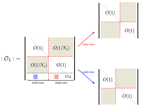
Figure 3: The structure of the Gram-Schmidt determinant at large Ncsubscript𝑁𝑐N_{c}. Owing to the large Ncsubscript𝑁𝑐N_{c} scaling of the two-point functions (3.24), the Gram-Schmidt matrix for :𝒪L::\!\mathcal{O}_{L}\!:\, consist of O(1)𝑂1O(1) diagonal blocks and O(1/Nc)𝑂1subscript𝑁𝑐O(1/N_{c}) off-diagonal blocks. To faciliate seeing the structure of the matrix, we drew gray dashed lines which indicate the diagonal entries. To read off the contribution of each bare operator, one needs to compute cofactors (minors) of the elements in the last row. The cofactor of the single-trace operator, an example of which is denoted by a red square in the matrix on the left, is given by the determinant at the top-right corner. As is clear from the figure, its diagonal entries are all O(1)𝑂1O(1). On the other hand, the cofactor of the multi-trace operator, an example of which is denoted by a blue square in the matrix on the left, is given by the determinant at the lower-right corner and is O(1/Nc)𝑂1subscript𝑁𝑐O(1/N_{c}).

Let us now prove the decoupling more rigorously from the structure of the Gram-Schmidt determinant (3.10). For this purpose, we simply need to use the fact that the inner product between the “single-trace” operator111111Namely the operators made up purely of insertions on the Wilson loop. 𝒪Lsubscript𝒪𝐿\mathcal{O}_{L} and the “multi-trace” operator 𝒪L|J1,,Jnsubscript𝒪conditionalsuperscript𝐿subscript𝐽1subscript𝐽𝑛\mathcal{O}_{L^{\prime}|J_{1},\ldots,J_{n}} is suppressed by 1/Nc1subscript𝑁𝑐1/N_{c}, which follows from the standard large Ncsubscript𝑁𝑐N_{c} counting:

(𝒪L,𝒪L|J1,,Jn)=𝒲[Φ~Φ~L+L]O^J1,,JnO(1/Nc).subscript𝒪𝐿subscript𝒪conditionalsuperscript𝐿subscript𝐽1subscript𝐽𝑛delimited-⟨⟩𝒲delimited-[]subscript~Φ~Φ𝐿superscript𝐿subscript^𝑂subscript𝐽1subscript𝐽𝑛similar-to𝑂1subscript𝑁𝑐(\mathcal{O}_{L}\,,\,\mathcal{O}_{L^{\prime}|J_{1},\ldots,J_{n}})=\langle\mathcal{W}[\underbracket{\tilde{\Phi}\cdots\tilde{\Phi}}_{L+L^{\prime}}]\,\hat{O}_{J_{1},\ldots,J_{n}}\rangle\sim O(1/N_{c})\,. (3.21)

To actually prove the decoupling, we first rearrange the rows and the columns of the determinant (3.10) and express the operator :𝒪L::\!\mathcal{O}_{L}\!:\, as shown in figure 3. Then, using the large Ncsubscript𝑁𝑐N_{c} scaling for the inner products (3.21), one can show that the off-diagonal blocks (shaded rectangular regions in figure 3) are all of order O(1/Nc)𝑂1subscript𝑁𝑐O(1/N_{c}) or higher while the diagonal blocks are of order 111. Now, the coefficient multiplying each bare operator can be read off from the cofactors (also known as minors) of the elements in the last row. As shown in figure 3, the cofactors of the insertions on the loop, 𝒪Lsubscript𝒪superscript𝐿\typecolon\mathcal{O}_{L^{\prime}}\typecolon are O(1)𝑂1O(1) since their diagonal entries are all O(1)𝑂1O(1). On the other hand, the cofactors of the multi-trace operators are at most O(1/Nc)𝑂1subscript𝑁𝑐O(1/N_{c}) since one always needs to take at least one O(1/Nc)𝑂1subscript𝑁𝑐O(1/N_{c}) element when computing the determinant. This shows that, in the strict large Ncsubscript𝑁𝑐N_{c} limit, the contribution from the multi-trace operators to the single-trace operators is negligible and one can therefore focus on the insertions on the Wilson loop.

Now, after the decoupling of all the multi-trace operators, the Gram-Schmidt analysis simplifies greatly since there is only one operator left for each R𝑅R-charge. We thus obtain the following expression for the normal-ordered insertions at large Ncsubscript𝑁𝑐N_{c},

𝒪L1DL|WW1WLW1W2WL+1WL1WLW2L1𝒪0𝒪1𝒪L|,DLdetWi+j2i,j(1i,jL),formulae-sequencesubscript𝒪𝐿1subscript𝐷𝐿𝑊subscript𝑊1subscript𝑊𝐿subscript𝑊1subscript𝑊2subscript𝑊𝐿1subscript𝑊𝐿1subscript𝑊𝐿subscript𝑊2𝐿1subscript𝒪0subscript𝒪1subscript𝒪𝐿subscript𝐷𝐿subscriptsubscript𝑊𝑖𝑗2𝑖𝑗formulae-sequence1𝑖𝑗𝐿\typecolon\mathcal{O}_{L}\typecolon\equiv\frac{1}{D_{L}}\left|\begin{array}[]{cccc}W&W_{1}&\cdots&W_{L}\\ W_{1}&W_{2}&\cdots&W_{L+1}\\ \vdots&\vdots&\ddots&\vdots\\ W_{L-1}&W_{L}&\cdots&W_{2L-1}\\ \mathcal{O}_{0}&\mathcal{O}_{1}&\cdots&\mathcal{O}_{L}\end{array}\right|\,,\qquad D_{L}\equiv\det{}_{i,j}W_{i+j-2}\quad(1\leq i,j\leq L)\,, (3.22)

where 𝒪Lsubscript𝒪𝐿\mathcal{O}_{L} is given by (3.12), namely 𝒪L𝒲[Φ~L]subscript𝒪𝐿𝒲delimited-[]superscript~Φ𝐿\mathcal{O}_{L}\equiv\mathcal{W}[\tilde{\Phi}^{L}], and the symbol \typecolon\ast\typecolon denotes the normal ordering at large Ncsubscript𝑁𝑐N_{c}. This is precisely the expression we derived in the previous paper [18], which correctly reproduces the perturbative results at weak and strong coupling.

For the analysis of the subleading corrections which we perform below, it is helpful to extend the definition of the large-Ncsubscript𝑁𝑐N_{c} normal ordering also to the multi-trace operators. The extension is simple; we simply define them as a product of 𝒪Lsubscript𝒪𝐿\typecolon\mathcal{O}_{L}\typecolon and the bulk multi-trace operator:

𝒪L|J1,,Jn𝒪LO^J1,,Jn.subscript𝒪conditional𝐿subscript𝐽1subscript𝐽𝑛subscript𝒪𝐿subscript^𝑂subscript𝐽1subscript𝐽𝑛\typecolon\mathcal{O}_{L|J_{1},\ldots,J_{n}}\typecolon\equiv\typecolon\mathcal{O}_{L}\typecolon\,\,\hat{O}_{J_{1},\ldots,J_{n}}\,. (3.23)

One can easily check that these operators are orthogonal to each other at large Ncsubscript𝑁𝑐N_{c}, namely

(𝒪L|𝐉,𝒪L|𝐉){O(1)(L=L and 𝐉=𝐉)O(1/Nc) or higher(LL or 𝐉𝐉),similar-tosubscript𝒪conditional𝐿𝐉subscript𝒪conditionalsuperscript𝐿superscript𝐉cases𝑂1𝐿superscript𝐿 and 𝐉superscript𝐉𝑂1subscript𝑁𝑐 or higher𝐿superscript𝐿 or 𝐉superscript𝐉(\typecolon\mathcal{O}_{L|{\bf J}}\typecolon\,,\,\typecolon\mathcal{O}_{L^{\prime}|{\bf J}^{\prime}}\typecolon)\sim\begin{cases}O(1)\qquad&(L=L^{\prime}\text{ and }{\bf J}={\bf J}^{\prime})\\ O(1/N_{c})\text{ or higher}\qquad&(L\neq L^{\prime}\text{ or }{\bf J}\neq{\bf J}^{\prime})\end{cases}\,, (3.24)

where 𝐉𝐉{\bf J} and 𝐉superscript𝐉{\bf J}^{\prime} denote sets of J𝐽J’s, namely 𝐉={J1,,Jn}𝐉subscript𝐽1subscript𝐽𝑛{\bf J}=\{J_{1},\ldots,J_{n}\} and 𝐉={J1,,Jn}superscript𝐉subscriptsuperscript𝐽1subscriptsuperscript𝐽superscript𝑛{\bf J}^{\prime}=\{J^{\prime}_{1},\ldots,{J}^{\prime}_{n^{\prime}}\}. In what follows, we use these operators as the basis for analyzing the subleading corrections.

Correction at O(1/Nc)𝑂1subscript𝑁𝑐O(1/N_{c})

At O(1/Nc)𝑂1subscript𝑁𝑐O(1/N_{c}), the operators 𝒪Lsubscript𝒪𝐿\typecolon\mathcal{O}_{L}\typecolon’s can mix with the double-trace operators 𝒪|j𝒲[Φ~]tr[Φ~j]similar-to-or-equalssubscript𝒪conditional𝑗𝒲delimited-[]superscript~Φtrdelimited-[]superscript~Φ𝑗\typecolon\mathcal{O}_{\ell|j}\typecolon\simeq\mathcal{W}[\tilde{\Phi}^{\ell}]{\rm tr}[\tilde{\Phi}^{j}] since their two-point functions, or equivalently the inner products in the Gram-Schmidt language, are no longer orthogonal at O(1/Nc)𝑂1subscript𝑁𝑐O(1/N_{c}):

𝒪L𝒪|j=WL+|j+O(1/Nc).delimited-⟨⟩subscript𝒪𝐿subscript𝒪conditional𝑗subscript𝑊𝐿conditional𝑗similar-to𝑂1subscript𝑁𝑐\langle\typecolon\mathcal{O}_{L}\typecolon\typecolon\mathcal{O}_{\ell|j}\typecolon\rangle=W_{L+\ell|j}+\cdots\,\,\sim\,\,O(1/N_{c})\,. (3.25)

To restore the orthogonality, we need perform the following subtraction from 𝒪Lsubscript𝒪𝐿\typecolon\mathcal{O}_{L}\typecolon,

:𝒪L:=𝒪LS1+O(1/Nc2),:\!\mathcal{O}_{L}\!:\,=\typecolon\mathcal{O}_{L}\typecolon-S_{1}+O(1/N_{c}^{2})\,, (3.26)

where S1subscript𝑆1S_{1} is O(1/Nc)𝑂1subscript𝑁𝑐O(1/N_{c}) and is given by

S1=+j<L0, 1j𝒪𝒪|j𝒪|j𝒪|j𝒪|j.subscript𝑆1subscript𝑗𝐿formulae-sequence01𝑗delimited-⟨⟩subscript𝒪subscript𝒪conditional𝑗delimited-⟨⟩subscript𝒪conditional𝑗subscript𝒪conditional𝑗subscript𝒪conditional𝑗S_{1}=\sum_{\begin{subarray}{c}\ell+j<L\\ 0\leq\ell,\,1\leq j\end{subarray}}\frac{\langle\typecolon\mathcal{O}_{\ell}\typecolon\typecolon\mathcal{O}_{\ell|j}\typecolon\rangle}{\langle\typecolon\mathcal{O}_{\ell|j}\typecolon\typecolon\mathcal{O}_{\ell|j}\typecolon\rangle}\typecolon\mathcal{O}_{\ell|j}\typecolon\,. (3.27)

Here the summation range is restricted to +j<L𝑗𝐿\ell+j<L since the self-contraction of L𝐿L single-letter insertions only produces the operators with charge smaller than L𝐿L as was exemplified in section 3.1. At this order, there is no need for further subtraction since the two-point functions with higher-trace operators are O(1/Nc2)𝑂1superscriptsubscript𝑁𝑐2O(1/N_{c}^{2}) or higher121212This can be shown from the standard large Ncsubscript𝑁𝑐N_{c} counting. and their mixing effects can be neglected. As we will see in section 4, the subtraction (3.26) is necessary in order to reproduce the correct bulk-defect correlators.

Correction at O(1/Nc2)𝑂1superscriptsubscript𝑁𝑐2O(1/N_{c}^{2})

Now at the next order, there are several sources of corrections. Firstly, the operator 𝒪Lsubscript𝒪𝐿\typecolon\mathcal{O}_{L}\typecolon can now mix with the triple-trace operators 𝒪|{j1,j2}subscript𝒪conditionalsubscript𝑗1subscript𝑗2\typecolon\mathcal{O}_{\ell|\{j_{1},j_{2}\}}\typecolon. This mixing can be resolved by subtracting the following term from 𝒪Lsubscript𝒪𝐿\typecolon\mathcal{O}_{L}\typecolon:

S2(1)=+j1+j2<L0, 1j1,j2𝒪L𝒪|j1,j2𝒪|j1,j2𝒪|j1,j2𝒪|j1,j2.superscriptsubscript𝑆21subscriptsubscript𝑗1subscript𝑗2𝐿formulae-sequence01subscript𝑗1subscript𝑗2delimited-⟨⟩subscript𝒪𝐿subscript𝒪conditionalsubscript𝑗1subscript𝑗2delimited-⟨⟩subscript𝒪conditionalsubscript𝑗1subscript𝑗2subscript𝒪conditionalsubscript𝑗1subscript𝑗2subscript𝒪conditionalsubscript𝑗1subscript𝑗2S_{2}^{(1)}=\sum_{\begin{subarray}{c}\ell+j_{1}+j_{2}<L\\ 0\leq\ell,\,1\leq j_{1},j_{2}\end{subarray}}\frac{\langle\typecolon\mathcal{O}_{L}\typecolon\typecolon\mathcal{O}_{\ell|j_{1},j_{2}}\typecolon\rangle}{\langle\typecolon\mathcal{O}_{\ell|j_{1},j_{2}}\typecolon\typecolon\mathcal{O}_{\ell|j_{1},j_{2}}\typecolon\rangle}\typecolon\mathcal{O}_{\ell|j_{1},j_{2}}\typecolon\,. (3.28)

Secondly, because of the subtraction added at O(1/Nc)𝑂1subscript𝑁𝑐O(1/N_{c}) (3.26), different 𝒪Lsubscript𝒪𝐿\typecolon\mathcal{O}_{L}\typecolon’s are no longer orthogonal to each other. For instance the two-point function of :𝒪L::\!\mathcal{O}_{L}\!:\, and :𝒪~::\!\mathcal{O}_{\tilde{\ell}}\!:\, (L~𝐿~L\neq\tilde{\ell}) is given by

:𝒪L:|1/Nc:𝒪~:|1/Nc=\displaystyle\langle\left.:\!\mathcal{O}_{L}\!:\,\right|_{1/N_{c}}\left.:\!\mathcal{O}_{\tilde{\ell}}\!:\,\right|_{1/N_{c}}\rangle= +j<L0, 1j𝒪L𝒪|j𝒪~𝒪|j𝒪|j𝒪|jsubscript𝑗𝐿formulae-sequence01𝑗delimited-⟨⟩subscript𝒪𝐿subscript𝒪conditional𝑗delimited-⟨⟩subscript𝒪~subscript𝒪conditional𝑗delimited-⟨⟩subscript𝒪conditional𝑗subscript𝒪conditional𝑗\displaystyle-\sum_{\begin{subarray}{c}\ell+j<L\\ 0\leq\ell,\,1\leq j\end{subarray}}\frac{\langle\typecolon\mathcal{O}_{L}\typecolon\typecolon\mathcal{O}_{\ell|j}\typecolon\rangle\langle\typecolon\mathcal{O}_{\tilde{\ell}}\typecolon\typecolon\mathcal{O}_{\ell|j}\typecolon\rangle}{\langle\typecolon\mathcal{O}_{\ell|j}\typecolon\typecolon\mathcal{O}_{\ell|j}\typecolon\rangle} (3.29)
+j<~0, 1j𝒪L𝒪|j𝒪~𝒪|j𝒪|j𝒪|jsubscript𝑗~formulae-sequence01𝑗delimited-⟨⟩subscript𝒪𝐿subscript𝒪conditional𝑗delimited-⟨⟩subscript𝒪~subscript𝒪conditional𝑗delimited-⟨⟩subscript𝒪conditional𝑗subscript𝒪conditional𝑗\displaystyle-\sum_{\begin{subarray}{c}\ell+j<\tilde{\ell}\\ 0\leq\ell,\,1\leq j\end{subarray}}\frac{\langle\typecolon\mathcal{O}_{L}\typecolon\typecolon\mathcal{O}_{\ell|j}\typecolon\rangle\langle\typecolon\mathcal{O}_{\tilde{\ell}}\typecolon\typecolon\mathcal{O}_{\ell|j}\typecolon\rangle}{\langle\typecolon\mathcal{O}_{\ell|j}\typecolon\typecolon\mathcal{O}_{\ell|j}\typecolon\rangle}
++j<L,~0, 1j𝒪L𝒪|j𝒪~𝒪|j𝒪|j𝒪|j.subscript𝑗𝐿~formulae-sequence01𝑗delimited-⟨⟩subscript𝒪𝐿subscript𝒪conditional𝑗delimited-⟨⟩subscript𝒪~subscript𝒪conditional𝑗delimited-⟨⟩subscript𝒪conditional𝑗subscript𝒪conditional𝑗\displaystyle+\sum_{\begin{subarray}{c}\ell+j<L,\tilde{\ell}\\ 0\leq\ell,\,1\leq j\end{subarray}}\frac{\langle\typecolon\mathcal{O}_{L}\typecolon\typecolon\mathcal{O}_{\ell|j}\typecolon\rangle\langle\typecolon\mathcal{O}_{\tilde{\ell}}\typecolon\typecolon\mathcal{O}_{\ell|j}\typecolon\rangle}{\langle\typecolon\mathcal{O}_{\ell|j}\typecolon\typecolon\mathcal{O}_{\ell|j}\typecolon\rangle}\,.

Here, the first and the second terms come from the O(1/Nc)𝑂1subscript𝑁𝑐O(1/N_{c}) corrections to 𝒪Lsubscript𝒪𝐿\typecolon\mathcal{O}_{L}\typecolon and 𝒪~subscript𝒪~\typecolon\mathcal{O}_{\tilde{\ell}}\typecolon while the third term comes from the corrections to both of the operators.

One can restore the orthogonality by further subtracting the following term from 𝒪Lsubscript𝒪𝐿\typecolon\mathcal{O}_{L}\typecolon:

S2(2)=~<L+j<L𝒪L,𝒪|j𝒪~𝒪|j𝒪|j𝒪|j𝒪~𝒪~𝒪~.superscriptsubscript𝑆22subscript~𝐿subscript𝑗𝐿subscript𝒪𝐿subscript𝒪conditional𝑗delimited-⟨⟩subscript𝒪~subscript𝒪conditional𝑗delimited-⟨⟩subscript𝒪conditional𝑗subscript𝒪conditional𝑗delimited-⟨⟩subscript𝒪~subscript𝒪~subscript𝒪~S_{2}^{(2)}=-\sum_{\tilde{\ell}<L}\,\,\,\sum_{\ell+j<L}\frac{\langle\typecolon\mathcal{O}_{L}\typecolon,\typecolon\mathcal{O}_{\ell|j}\typecolon\rangle\langle\typecolon\mathcal{O}_{\tilde{\ell}}\typecolon\typecolon\mathcal{O}_{\ell|j}\typecolon\rangle}{\langle\typecolon\mathcal{O}_{\ell|j}\typecolon\typecolon\mathcal{O}_{\ell|j}\typecolon\rangle\langle\typecolon\mathcal{O}_{\tilde{\ell}}\typecolon\typecolon\mathcal{O}_{\tilde{\ell}}\typecolon\rangle}\typecolon\mathcal{O}_{\tilde{\ell}}\typecolon\,. (3.30)

Again the summation range is restricted to ~<L~𝐿\tilde{\ell}<L due to the structure of the self-contraction.

The last correction comes from the O(1/Nc2)𝑂1superscriptsubscript𝑁𝑐2O(1/N_{c}^{2}) correction to the expectation value of the Wilson loop and its derivatives Wksubscript𝑊𝑘W_{k}. This correction can be easily taken into account by taking the expression (3.22), and expand it to the next order.

Therefore, everything combined, we obtain the following expression for :𝒪L::\!\mathcal{O}_{L}\!:\, at O(1/Nc2)𝑂1superscriptsubscript𝑁𝑐2O(1/N_{c}^{2}):

:𝒪L:=𝒪L|1/Nc2S1O(1/Nc)(S2(1)+S2(2))O(1/Nc2)+O(1/Nc3).\displaystyle:\!\mathcal{O}_{L}\!:\,=\left.\typecolon\mathcal{O}_{L}\typecolon\right|_{1/N_{c}^{2}}-\underbrace{S_{1}}_{O(1/N_{c})}-\underbrace{(S_{2}^{(1)}+S_{2}^{(2)})}_{O(1/N_{c}^{2})}+O(1/N_{c}^{3})\,. (3.31)

Here the notation 𝒪L|1/Nc2evaluated-atsubscript𝒪𝐿1superscriptsubscript𝑁𝑐2\left.\typecolon\mathcal{O}_{L}\typecolon\right|_{1/N_{c}^{2}} denotes the determinant (3.22) expanded up to O(1/Nc2)𝑂1superscriptsubscript𝑁𝑐2O(1/N_{c}^{2}). In section 6, we will use this expression to compute the corrections to the correlators on the Wilson loop and check them against the direct perturbative computation.

4 Bulk-defect correlators at large Ncsubscript𝑁𝑐N_{c}

In this section, we compute the bulk-defect correlators

GL|J𝒲[:Φ~L:]O^J,G_{L|J}\equiv\langle\mathcal{W}[:\!\tilde{\Phi}^{L}\!:\,]\,\,\hat{O}_{J}\rangle\,, (4.1)

at large Ncsubscript𝑁𝑐N_{c} using the normal-ordered operators that we constructed in the previous section. Generalization to two operator insertions on the Wilson loop, namely

GL1,L2|J𝒲[:Φ~L1::Φ~L2:]O^J,G_{L_{1},L_{2}|J}\equiv\langle\mathcal{W}[:\!\tilde{\Phi}^{L_{1}}\!:\,:\!\tilde{\Phi}^{L_{2}}\!:\,]\,\,\hat{O}_{J}\rangle\,, (4.2)

will be presented in Appendix B.

4.1 Generalities

To compute the result at large Ncsubscript𝑁𝑐N_{c}, we simply need to substitute the large Ncsubscript𝑁𝑐N_{c} expansion of :Φ~L:=:𝒪L::\!\tilde{\Phi}^{L}\!:\,=:\!\mathcal{O}_{L}\!:\, (3.26) to (4.1). The result is

GL|J=𝒪LO^JL1+J1<L0L1, 1J1𝒪L𝒪L1|J1𝒪L1|J1𝒪L1|J1O(1/Nc)𝒪L1|J1O^JO(1) or O(1/Nc)+O(1/Nc2).subscript𝐺conditional𝐿𝐽delimited-⟨⟩subscript𝒪𝐿subscript^𝑂𝐽subscriptsubscript𝐿1subscript𝐽1𝐿formulae-sequence0subscript𝐿11subscript𝐽1subscriptdelimited-⟨⟩subscript𝒪𝐿subscript𝒪conditionalsubscript𝐿1subscript𝐽1delimited-⟨⟩subscript𝒪conditionalsubscript𝐿1subscript𝐽1subscript𝒪conditionalsubscript𝐿1subscript𝐽1𝑂1subscript𝑁𝑐subscriptdelimited-⟨⟩subscript𝒪conditionalsubscript𝐿1subscript𝐽1subscript^𝑂𝐽𝑂1 or 𝑂1subscript𝑁𝑐𝑂1superscriptsubscript𝑁𝑐2G_{L|J}=\langle\typecolon\mathcal{O}_{L}\typecolon\hat{O}_{J}\rangle-\sum_{\begin{subarray}{c}L_{1}+J_{1}<L\\ 0\leq L_{1},\,1\leq J_{1}\end{subarray}}\underbrace{\frac{\langle\typecolon\mathcal{O}_{L}\typecolon\typecolon\mathcal{O}_{L_{1}|J_{1}}\typecolon\rangle}{\langle\typecolon\mathcal{O}_{L_{1}|J_{1}}\typecolon\typecolon\mathcal{O}_{L_{1}|J_{1}}\typecolon\rangle}}_{O(1/N_{c})}\underbrace{\langle\typecolon\mathcal{O}_{L_{1}|J_{1}}\typecolon\hat{O}_{J}\rangle}_{O(1)\text{ or }O(1/N_{c})}+O(1/N_{c}^{2})\,. (4.3)

As indicated, the first factor in the sum is always O(1/Nc)𝑂1subscript𝑁𝑐O(1/N_{c}) due to the large Ncsubscript𝑁𝑐N_{c} scaling given in (3.24). On the other hand, the second factor in the sum is O(1)𝑂1O(1) if J1=Jsubscript𝐽1𝐽J_{1}=J and L1=0subscript𝐿10L_{1}=0 while in all the other cases it is O(1/Nc)𝑂1subscript𝑁𝑐O(1/N_{c}). Owing to the range of summation, the case with J1=Jsubscript𝐽1𝐽J_{1}=J and L1=0subscript𝐿10L_{1}=0 is included in the sum only if J<L𝐽𝐿J<L, and when it is included it just kills the leading term 𝒪LO^Jdelimited-⟨⟩subscript𝒪𝐿subscript^𝑂𝐽\langle\typecolon\mathcal{O}_{L}\typecolon\hat{O}_{J}\rangle. Therefore we arrive at the following result:

GL|J={0(J<L)𝒪LO^J+O(1/Nc2)(JL).subscript𝐺conditional𝐿𝐽cases0𝐽𝐿delimited-⟨⟩subscript𝒪𝐿subscript^𝑂𝐽𝑂1superscriptsubscript𝑁𝑐2𝐽𝐿\displaystyle G_{L|J}=\begin{cases}0&\qquad(J<L)\\ \langle\typecolon\mathcal{O}_{L}\typecolon\hat{O}_{J}\rangle+O(1/N_{c}^{2})&\qquad(J\geq L)\end{cases}\,. (4.4)

In fact GL|Jsubscript𝐺conditional𝐿𝐽G_{L|J} for J<L𝐽𝐿J<L actually vanishes at any order of the 1/Nc1subscript𝑁𝑐1/N_{c} expansion, not just at the leading order. This is easy to see in the case of the 1/2-BPS Wilson loop from R𝑅R-symmetry selection rules, but it is also true in the general 1/8181/8-BPS case.131313This can be seen to follow from the structure of the Gram-Schmidt process. Indeed, by using the bulk-defect OPE, one can express the bulk operator O^Jsubscript^𝑂𝐽\hat{O}_{J} as a sum of defect operators with charges smaller than or equal to J𝐽J. As a result, the bulk-defect correlator is given by a sum of the defect two-point functions. One can then use the orthogonality of the normal-ordered defect operators constructed in the Gram-Schmidt process to show that all these two-point functions vanish.

To compute the leading expression 𝒪LO^Jdelimited-⟨⟩subscript𝒪𝐿subscript^𝑂𝐽\langle\typecolon\mathcal{O}_{L}\typecolon\hat{O}_{J}\rangle, it is convenient to consider the following polynomial [18]:

FL(X)=1DL|WW1WLW1W2WL+1WL1WLW2L11XXL|.subscript𝐹𝐿𝑋1subscript𝐷𝐿𝑊subscript𝑊1subscript𝑊𝐿subscript𝑊1subscript𝑊2subscript𝑊𝐿1subscript𝑊𝐿1subscript𝑊𝐿subscript𝑊2𝐿11𝑋superscript𝑋𝐿F_{L}(X)=\frac{1}{D_{L}}\left|\begin{array}[]{cccc}W&W_{1}&\cdots&W_{L}\\ W_{1}&W_{2}&\cdots&W_{L+1}\\ \vdots&\vdots&\ddots&\vdots\\ W_{L-1}&W_{L}&\cdots&W_{2L-1}\\ 1&X&\cdots&X^{L}\end{array}\right|\,. (4.5)

This reproduces the expression for 𝒪Lsubscript𝒪𝐿\typecolon\mathcal{O}_{L}\typecolon (3.22) once we replace Xksuperscript𝑋𝑘X^{k} by 𝒪ksubscript𝒪𝑘\mathcal{O}_{k}. Now using the fact that the insertion of the bare operators 𝒪k(=Φ~k)annotatedsubscript𝒪𝑘absentsuperscript~Φ𝑘\mathcal{O}_{k}(=\tilde{\Phi}^{k}) can be traded for the area derivative Aksuperscriptsubscript𝐴𝑘\partial_{A}^{k}, one can write down the following expression for 𝒲[:Φ~L:]O^J\langle\mathcal{W}[:\!\tilde{\Phi}^{L}\!:\,]\hat{O}_{J}\rangle,

𝒲[:Φ~L:]O^J|Nc=𝒪LO^J=FL[A][𝒲O^J(A)]|A=A.\langle\mathcal{W}[:\!\tilde{\Phi}^{L}\!:\,]\hat{O}_{J}\rangle|_{N_{c}\to\infty}=\langle\typecolon\mathcal{O}_{L}\typecolon\hat{O}_{J}\rangle=F_{L}[\partial_{A^{\prime}}]\left.\left[\langle\mathcal{W}\hat{O}_{J}\rangle(A^{\prime})\right]\right|_{A^{\prime}=A}\,. (4.6)

Let us make some clarification of this formula: In (4.6), Asuperscript𝐴A^{\prime} is the area of the region inside the Wilson loop in 𝒲O^Jdelimited-⟨⟩𝒲subscript^𝑂𝐽\langle\mathcal{W}\hat{O}_{J}\rangle, and the area derivatives only act on 𝒲OJ(A)delimited-⟨⟩𝒲subscript𝑂𝐽superscript𝐴\langle\mathcal{W}O_{J}\rangle(A^{\prime}) not on the coefficients of FLsubscript𝐹𝐿F_{L}.

One can also generalize this expression to the correlators involving several operator insertions on a single Wilson loop. The result for the generalization reads

𝒲[k=1n:Φ~Lk:]O^J|Nc=k=1nFLk[A][𝒲O^J(A)]|A=A.\displaystyle\langle\mathcal{W}[\prod_{k=1}^{n}:\!\tilde{\Phi}^{L_{k}}\!:\,]\hat{O}_{J}\rangle|_{N_{c}\to\infty}=\prod_{k=1}^{n}F_{L_{k}}[\partial_{A^{\prime}}]\left.\left[\langle\mathcal{W}\hat{O}_{J}\rangle(A^{\prime})\right]\right|_{A^{\prime}=A}\,. (4.7)

For n3𝑛3n\geq 3, this expression is valid when JLi𝐽subscript𝐿𝑖J\geq L_{i} (i=1,,n)𝑖1𝑛(i=1,\ldots,n), and otherwise there are some corrections coming from the nonplanar corrections to :Φ~Lk::\!\tilde{\Phi}^{L_{k}}\!:\,. This rule is slightly modified for n=2𝑛2n=2 as will be discussed in Appendix B.

4.2 Integral representation and Quantum Spectral Curve

Let us now evaluate (4.6) more explicitly using the large Ncsubscript𝑁𝑐N_{c} expression for 𝒲O^Jdelimited-⟨⟩𝒲subscript^𝑂𝐽\langle\mathcal{W}\hat{O}_{J}\rangle given in (2.12). For this purpose, it is useful to consider the following generating series141414This can be derived from the usual generating function for the modified Bessel function, eλ2(y+1y)=nIn(λ)ynsuperscript𝑒superscript𝜆2𝑦1𝑦subscript𝑛subscript𝐼𝑛superscript𝜆superscript𝑦𝑛e^{\frac{\sqrt{\lambda^{\prime}}}{2}(y+\frac{1}{y})}=\sum_{n}I_{n}(\sqrt{\lambda^{\prime}})y^{n}, after the change of variables y=2π+a2πax𝑦2𝜋𝑎2𝜋𝑎𝑥y=\sqrt{\frac{2\pi+a}{2\pi-a}}x.

e2πg(x+1x)ega(x1x)=n=In(λ)(2π+a2πa)n/2xn,superscript𝑒2𝜋𝑔𝑥1𝑥superscript𝑒𝑔𝑎𝑥1𝑥superscriptsubscript𝑛subscript𝐼𝑛superscript𝜆superscript2𝜋𝑎2𝜋𝑎𝑛2superscript𝑥𝑛\displaystyle e^{2\pi g(x+\frac{1}{x})}e^{ga(x-\frac{1}{x})}=\sum_{n=-\infty}^{\infty}I_{n}(\sqrt{\lambda^{\prime}})\left(\frac{2\pi+a}{2\pi-a}\right)^{n/2}x^{n}\,, (4.8)

where g𝑔g is related to the ’t Hooft coupling λ𝜆\lambda as

gλ4π.𝑔𝜆4𝜋g\equiv\frac{\sqrt{\lambda}}{4\pi}\,. (4.9)

Using this generating series, 𝒲O^Jdelimited-⟨⟩𝒲subscript^𝑂𝐽\langle\mathcal{W}\hat{O}_{J}\rangle at large Ncsubscript𝑁𝑐N_{c} can be expressed as

𝒲O^J=2J/2JNcdxxJ12πie2πg(x+1x)ega(x1x).delimited-⟨⟩𝒲subscript^𝑂𝐽superscript2𝐽2𝐽subscript𝑁𝑐contour-integral𝑑𝑥superscript𝑥𝐽12𝜋𝑖superscript𝑒2𝜋𝑔𝑥1𝑥superscript𝑒𝑔𝑎𝑥1𝑥\displaystyle\langle\mathcal{W}\hat{O}_{J}\rangle=\frac{2^{-J/2}\sqrt{J}}{N_{c}}\oint\frac{dx\,x^{J-1}}{2\pi i}e^{2\pi g(x+\frac{1}{x})}e^{ga(x-\frac{1}{x})}\,. (4.10)

In this expression, the area-dependence only shows up in the exponent and we therefore have

(A)k𝒲O^J=2J/2JNcdxxJ12πigk(x1x)ke2πg(x+1x)ega(x1x).superscriptsubscript𝐴𝑘delimited-⟨⟩𝒲subscript^𝑂𝐽superscript2𝐽2𝐽subscript𝑁𝑐contour-integral𝑑𝑥superscript𝑥𝐽12𝜋𝑖superscript𝑔𝑘superscript𝑥1𝑥𝑘superscript𝑒2𝜋𝑔𝑥1𝑥superscript𝑒𝑔𝑎𝑥1𝑥(\partial_{A})^{k}\langle\mathcal{W}\hat{O}_{J}\rangle=\frac{2^{-J/2}\sqrt{J}}{N_{c}}\oint\frac{dx\,x^{J-1}}{2\pi i}g^{k}\left(x-\frac{1}{x}\right)^{k}e^{2\pi g(x+\frac{1}{x})}e^{ga(x-\frac{1}{x})}\,. (4.11)

We can then convert (4.6) into a simple integral expression

𝒲[:Φ~L:]O^J=2J/2JNcdμBJ(x)QL(x),\langle\mathcal{W}[:\!\tilde{\Phi}^{L}\!:\,]\hat{O}_{J}\rangle=\frac{2^{-J/2}\sqrt{J}}{N_{c}}\oint d\mu\,\,B_{J}(x)Q_{L}(x)\,, (4.12)

where dμ𝑑𝜇d\mu is the measure introduced in [18],

dμ=dx2πi1+x22e2πg(x+1x)ega(x1x)2πg,𝑑𝜇𝑑𝑥2𝜋𝑖1superscript𝑥22superscript𝑒2𝜋𝑔𝑥1𝑥superscript𝑒𝑔𝑎𝑥1𝑥2𝜋𝑔d\mu=\frac{dx}{2\pi i}\frac{1+x^{-2}}{2}\frac{e^{2\pi g(x+\frac{1}{x})}e^{ga(x-\frac{1}{x})}}{2\pi g}\,, (4.13)

and QL(x)subscript𝑄𝐿𝑥Q_{L}(x) and BJ(x)subscript𝐵𝐽𝑥B_{J}(x) are defined by

QL(x)FL(g(xx1)),BJ(x)=4πgxJ+11+x2.formulae-sequencesubscript𝑄𝐿𝑥subscript𝐹𝐿𝑔𝑥superscript𝑥1subscript𝐵𝐽𝑥4𝜋𝑔superscript𝑥𝐽11superscript𝑥2Q_{L}(x)\equiv F_{L}(g(x-x^{-1}))\,,\qquad B_{J}(x)=\frac{4\pi gx^{J+1}}{1+x^{2}}\,. (4.14)

As shown in [18], the functions QL(x)subscript𝑄𝐿𝑥Q_{L}(x)’s are orthogonal to each other under the measure μ𝜇\mu and their overlap integral gives the planar two-point function of the operators on the Wilson loop:

𝒲[:Φ~L::Φ~L:]|planar=dμQL(x)QL(x)=DL+1DLδLL.\langle\mathcal{W}[:\!\tilde{\Phi}^{L}\!:\,\,\,:\!\tilde{\Phi}^{L^{\prime}}\!:\,]\rangle|_{\rm planar}=\oint d\mu\,\,Q_{L}(x)Q_{L^{\prime}}(x)=\frac{D_{L+1}}{D_{L}}\delta_{L\,L^{\prime}}\,. (4.15)

Furthermore, QL(x)subscript𝑄𝐿𝑥Q_{L}(x) coincides with the so-called Q𝑄Q-function in the Quantum Spectral Curve formalism151515The same orthogonal polynomials appeared before in the integrability-based analysis of the operator spectrum on the Wilson loop [43, 44]. [45, 28]. The appearance of the Quantum Spectral Curve in (4.12) is rather striking and indicates the existence of the integrability-based description for the bulk-defect correlators. We will come back to this point in the conclusion.

One can also write down the result for multiple operator insertions on the Wilson loop. The result reads

𝒲[k=1n:Φ~Lk:]O^J=2J/2JNcdμBJ(x)k=1nQLk(x).\langle\mathcal{W}[\prod_{k=1}^{n}:\!\tilde{\Phi}^{L_{k}}\!:\,]\hat{O}_{J}\rangle=\frac{2^{-J/2}\sqrt{J}}{N_{c}}\oint d\mu\,\,B_{J}(x)\prod_{k=1}^{n}Q_{L_{k}}(x)\,. (4.16)

In what follows, we focus on the case of the 1/2121/2-BPS circular Wilson loop (namely we set a=0𝑎0a=0) and derive the weak- and the strong-coupling expansions of the integral (4.12).

4.3 Weak coupling expansion

To perform the weak-coupling expansion of the integral (4.12), we need to expand both the functions QLsubscript𝑄𝐿Q_{L} and BJsubscript𝐵𝐽B_{J}, and the measure μ𝜇\mu. The expansion of QLsubscript𝑄𝐿Q_{L} was computed in [18] and it reads

QL=(ig)L(UL(cosθ)+g22π23UL2(cosθ)+),subscript𝑄𝐿superscript𝑖𝑔𝐿subscript𝑈𝐿𝜃superscript𝑔22superscript𝜋23subscript𝑈𝐿2𝜃Q_{L}=(-ig)^{L}\left(U_{L}(\cos\theta)+g^{2}\frac{2\pi^{2}}{3}U_{L-2}(\cos\theta)+\cdots\right)\,, (4.17)

where ULsubscript𝑈𝐿U_{L} is the Chebyshev polynomial of the second kind and θ𝜃\theta is related to x𝑥x by

x=ieiθ.𝑥𝑖superscript𝑒𝑖𝜃x=-ie^{i\theta}\,. (4.18)

In terms of the variable θ𝜃\theta, the measure dμ𝑑𝜇d\mu, BLsubscript𝐵𝐿B_{L} and their product read161616 Note that we already set a=0𝑎0a=0 since we are studying the 1/2121/2-BPS Wilson loop.

dμ=dθsinθ4π2ge4πgsinθ,BJ=2πgsinθeiJθiJ,dμBJ=dθe4πgsinθ2πeiJθiJ,formulae-sequence𝑑𝜇𝑑𝜃𝜃4superscript𝜋2𝑔superscript𝑒4𝜋𝑔𝜃formulae-sequencesubscript𝐵𝐽2𝜋𝑔𝜃superscript𝑒𝑖𝐽𝜃superscript𝑖𝐽𝑑𝜇subscript𝐵𝐽𝑑𝜃superscript𝑒4𝜋𝑔𝜃2𝜋superscript𝑒𝑖𝐽𝜃superscript𝑖𝐽\displaystyle d\mu=\frac{d\theta\sin\theta}{4\pi^{2}g}e^{4\pi g\sin\theta}\,,\qquad B_{J}=\frac{2\pi g}{\sin\theta}\frac{e^{iJ\theta}}{i^{J}}\,,\qquad d\mu\,\,B_{J}=\frac{d\theta\,e^{4\pi g\sin\theta}}{2\pi}\frac{e^{iJ\theta}}{i^{J}}\,, (4.19)

and the weak-coupling expansion corresponds to expanding the exponential e2gsinθsuperscript𝑒2𝑔𝜃e^{2g\sin\theta}. Since ULsubscript𝑈𝐿U_{L} is an order L𝐿L polynomial, one has to expand e2gsinθsuperscript𝑒2𝑔𝜃e^{2g\sin\theta} up to the O(gJL)𝑂superscript𝑔𝐽𝐿O(g^{J-L}) term in order to compensate the factor eiJθsuperscript𝑒𝑖𝐽𝜃e^{iJ\theta} and get a non-zero integral:

dμBJ=dθ2πeiJθiJ(1++gJL2JL(2π)JL(JL)!sinJLθ+).𝑑𝜇subscript𝐵𝐽𝑑𝜃2𝜋superscript𝑒𝑖𝐽𝜃superscript𝑖𝐽1superscript𝑔𝐽𝐿superscript2𝐽𝐿superscript2𝜋𝐽𝐿𝐽𝐿superscript𝐽𝐿𝜃d\mu\,\,B_{J}=\frac{d\theta}{2\pi}\frac{e^{iJ\theta}}{i^{J}}\left(1+\cdots+g^{J-L}\frac{2^{J-L}(2\pi)^{J-L}}{(J-L)!}\sin^{J-L}\theta+\cdots\right)\,. (4.20)

Plugging in that term in the integral, we get

𝒲[:Φ~L:]O^J|leading\displaystyle\langle\mathcal{W}[:\!\tilde{\Phi}^{L}\!:\,]\hat{O}_{J}\rangle|_{\rm leading} =2J/2JNc(i)J+L(4π)JLgJ(JL)!dθ2πeiJθsinJLθUL(cosθ)absentsuperscript2𝐽2𝐽subscript𝑁𝑐superscript𝑖𝐽𝐿superscript4𝜋𝐽𝐿superscript𝑔𝐽𝐽𝐿𝑑𝜃2𝜋superscript𝑒𝑖𝐽𝜃superscript𝐽𝐿𝜃subscript𝑈𝐿𝜃\displaystyle=\frac{2^{-J/2}\sqrt{J}}{N_{c}}(-i)^{J+L}\frac{(4\pi)^{J-L}g^{J}}{(J-L)!}\int\frac{d\theta}{2\pi}e^{iJ\theta}\sin^{J-L}\theta\,\,U_{L}(\cos\theta) (4.21)
=(1)L2J/2JgJNc(2π)JL(JL)!,absentsuperscript1𝐿superscript2𝐽2𝐽superscript𝑔𝐽subscript𝑁𝑐superscript2𝜋𝐽𝐿𝐽𝐿\displaystyle=\frac{(-1)^{L}2^{-J/2}\sqrt{J}g^{J}}{N_{c}}\frac{(2\pi)^{J-L}}{(J-L)!}\,,

where we used in the second equality,

UL(cosθ)=sin(L+1)θsinθ.subscript𝑈𝐿𝜃𝐿1𝜃𝜃U_{L}(\cos\theta)=\frac{\sin(L+1)\theta}{\sin\theta}\,. (4.22)

One can also compute the higher orders in the expansion. At the order O(gJ+1)𝑂superscript𝑔𝐽1O(g^{J+1}), one can show by explicit computation that the contribution vanishes. This is of course in line with the perturbation theory in which the corrections always come with even powers of g𝑔g (recall that gλproportional-to𝑔𝜆g\propto\sqrt{\lambda}). Now, at the order O(gJ+2)𝑂superscript𝑔𝐽2O(g^{J+2}), the contribution only comes from the correction to dμBJ𝑑𝜇subscript𝐵𝐽d\mu\,\,B_{J}, not from the correction to QLsubscript𝑄𝐿Q_{L}171717The correction to QLsubscript𝑄𝐿Q_{L} is of O(gL+2)𝑂superscript𝑔𝐿2O(g^{L+2}) and proportional to UL2subscript𝑈𝐿2U_{L-2}. In order to make the integral involving UL2subscript𝑈𝐿2U_{L-2} nonvanishing, we need to take the O(gJL+2)𝑂superscript𝑔𝐽𝐿2O(g^{J-L+2}) term in the expansion of dμBJ𝑑𝜇subscript𝐵𝐽d\mu\,\,B_{J}. In total, it is of order O(gJ+4)𝑂superscript𝑔𝐽4O(g^{J+4}).. Thus the result reads

𝒲[:Φ~L:]O^J|next\displaystyle\langle\mathcal{W}[:\!\tilde{\Phi}^{L}\!:\,]\hat{O}_{J}\rangle|_{\rm next} =2J/2JNc(i)J+L(4π)JL+2gJ+2(JL+2)!dθ2πeiJθsinJL+2θUL(cosθ)absentsuperscript2𝐽2𝐽subscript𝑁𝑐superscript𝑖𝐽𝐿superscript4𝜋𝐽𝐿2superscript𝑔𝐽2𝐽𝐿2𝑑𝜃2𝜋superscript𝑒𝑖𝐽𝜃superscript𝐽𝐿2𝜃subscript𝑈𝐿𝜃\displaystyle=\frac{2^{-J/2}\sqrt{J}}{N_{c}}(-i)^{J+L}\frac{(4\pi)^{J-L+2}g^{J+2}}{(J-L+2)!}\int\frac{d\theta}{2\pi}e^{iJ\theta}\sin^{J-L+2}\theta\,\,U_{L}(\cos\theta) (4.23)
=(1)L2J/2JgJ+2Nc(JL)!(2π)JL+2JL+2.absentsuperscript1𝐿superscript2𝐽2𝐽superscript𝑔𝐽2subscript𝑁𝑐𝐽𝐿superscript2𝜋𝐽𝐿2𝐽𝐿2\displaystyle=\frac{(-1)^{L}2^{-J/2}\sqrt{J}g^{J+2}}{N_{c}(J-L)!}\frac{(2\pi)^{J-L+2}}{J-L+2}\,.

Here in the second equality we assumed L𝐿L is strictly larger than 00. We will comment on this point later in this section.

By dividing these results by the expectation of the Wilson loop,

𝒲=1+2π2g2+,delimited-⟨⟩𝒲12superscript𝜋2superscript𝑔2\langle\mathcal{W}\rangle=1+2\pi^{2}g^{2}+\cdots\,, (4.24)

we obtain the normalized correlators

𝒲[:Φ~L:]O^J=(1)L2J/2JgJNc(2π)JL(JL)![12π2g2JLJL+2+O(g4)].\langle\!\langle\mathcal{W}[:\!\tilde{\Phi}^{L}\!:\,]\hat{O}_{J}\rangle\!\rangle=\frac{(-1)^{L}2^{-J/2}\sqrt{J}g^{J}}{N_{c}}\frac{(2\pi)^{J-L}}{(J-L)!}\left[1-2\pi^{2}g^{2}\frac{J-L}{J-L+2}+O(g^{4})\right]\,. (4.25)

We can then read off the defect CFT data using the relations (2.26) and (2.27) as

cL|Jsubscript𝑐conditional𝐿𝐽\displaystyle c_{L|J} =2LJ2JgJNc(2π)JL(JL)![12π2g2JLJL+2+O(g4)],absentsuperscript2𝐿𝐽2𝐽superscript𝑔𝐽subscript𝑁𝑐superscript2𝜋𝐽𝐿𝐽𝐿delimited-[]12superscript𝜋2superscript𝑔2𝐽𝐿𝐽𝐿2𝑂superscript𝑔4\displaystyle=\frac{2^{L-\frac{J}{2}}\sqrt{J}g^{J}}{N_{c}}\frac{(2\pi)^{J-L}}{(J-L)!}\left[1-2\pi^{2}g^{2}\frac{J-L}{J-L+2}+O(g^{4})\right]\,, (4.26)
CL|Jsubscript𝐶conditional𝐿𝐽\displaystyle C_{L|J} =2LJ2(i)LJgJLNc(2π)JL(JL)![12π2g2(JLJL+213)+O(g4)],absentsuperscript2𝐿𝐽2superscript𝑖𝐿𝐽superscript𝑔𝐽𝐿subscript𝑁𝑐superscript2𝜋𝐽𝐿𝐽𝐿delimited-[]12superscript𝜋2superscript𝑔2𝐽𝐿𝐽𝐿213𝑂superscript𝑔4\displaystyle=\frac{2^{L-\frac{J}{2}}(-i)^{L}\sqrt{J}g^{J-L}}{N_{c}}\frac{(2\pi)^{J-L}}{(J-L)!}\left[1-2\pi^{2}g^{2}\left(\frac{J-L}{J-L+2}-\frac{1}{3}\right)+O(g^{4})\right]\,,

where we used

nL=(g2)L[12π2g23+O(g4)],subscript𝑛𝐿superscriptsuperscript𝑔2𝐿delimited-[]12superscript𝜋2superscript𝑔23𝑂superscript𝑔4n_{L}=(-g^{2})^{L}\left[1-\frac{2\pi^{2}g^{2}}{3}+O(g^{4})\right]\,, (4.27)

which was computed in [18]. As we will see in the next section, these results are in perfect agreement with the direct perturbative computation.
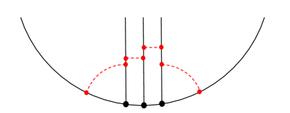
Refer to caption
Figure 4: An example of the wrapping diagram for the bulk-defect correlator. The black dots denote the field insertions Φ~~Φ\tilde{\Phi} and the black straight lines emanating from them are the propagators. When the loop order \ell is larger than L+1𝐿1L+1, one can connect the two edges of the Wilson loop (denoted by a black semi-circle) using a collection of gluon propagators (denoted by red dashed lines).

Before closing this section, let us make one remark: In the computation of the next-leading correction (4.23), we assumed that L𝐿L is strictly larger than zero. In that case one can replace UL=sin(L+1)θ/sinθsubscript𝑈𝐿𝐿1𝜃𝜃U_{L}=\sin(L+1)\theta/\sin\theta in the integrand with ei(L+1)θ/(2isinθ)superscript𝑒𝑖𝐿1𝜃2𝑖𝜃-e^{-i(L+1)\theta}/(2i\sin\theta) since the integral of the other exponential e+i(L+1)θ/(2isinθ)superscript𝑒𝑖𝐿1𝜃2𝑖𝜃e^{+i(L+1)\theta}/(2i\sin\theta) vanishes. On the other hand, for L=0𝐿0L=0 the other exponential does contribute and modifies the result to

𝒲O^J|nextevaluated-atdelimited-⟨⟩𝒲subscript^𝑂𝐽next\displaystyle\langle\mathcal{W}\hat{O}_{J}\rangle|_{\rm next} =2J/2JNc(i)J(4π)J+2gJ+2(J+2)!dθ2πeiJθsinJ+2θU0(cosθ)absentsuperscript2𝐽2𝐽subscript𝑁𝑐superscript𝑖𝐽superscript4𝜋𝐽2superscript𝑔𝐽2𝐽2𝑑𝜃2𝜋superscript𝑒𝑖𝐽𝜃superscript𝐽2𝜃subscript𝑈0𝜃\displaystyle=\frac{2^{-J/2}\sqrt{J}}{N_{c}}(-i)^{J}\frac{(4\pi)^{J+2}g^{J+2}}{(J+2)!}\int\frac{d\theta}{2\pi}e^{iJ\theta}\sin^{J+2}\theta\,\,U_{0}(\cos\theta) (4.28)
=2J/2J(2πg)J+2Nc(J+1)!.absentsuperscript2𝐽2𝐽superscript2𝜋𝑔𝐽2subscript𝑁𝑐𝐽1\displaystyle=\frac{2^{-J/2}\sqrt{J}(2\pi g)^{J+2}}{N_{c}(J+1)!}\,.

Because of this, one cannot simply analytically continue the L>0𝐿0L>0 result to get the result for L=0𝐿0L=0. More generally, at \ell loops, the other exponential starts to contribute when the length L𝐿L is equal to 11\ell-1 and the result therefore exhibits non-analyticity beyond that point. Although it might appear peculiar at first sight, such non-analyticity is not unheard of, and shows up also in the study of the anomalous dimensions181818An analogous phenomenon was found also for the structure constants of the single-trace operators [46]. of the single-trace operators [47, 48]; in that context, it is known that when the loop order exceeds the length of the operator a new type of planar diagrams which wrap around the operator show up and produce non-analyticity in the length L𝐿L. Such a phenomenon is called the wrapping correction.191919From the integrability point of view, these wrapping corrections correspond to the finite-size corrections which are produced by the virtual particles going around the spin chain [49]. This seems to be true also in our case since precisely at L=1𝐿1L=\ell-1 one can draw a new diagram which passes through the defect operator and connects the two edges of the Wilson loop (see figure 4). It would be interesting to make this connection more precise by directly analyzing the Feynman diagrams.

4.4 Strong coupling expansion

To perform the strong-coupling expansion, it is convenient to rewrite the integral in terms of

yi(xx1)2.𝑦𝑖𝑥superscript𝑥12y\equiv\frac{i(x-x^{-1})}{2}\,. (4.29)

The result after rewriting reads

𝑑μBJ=11dy2π1y2[(1y2iy)Je4πg1y2+(1y2iy)Je4πg1y2].\displaystyle\begin{aligned} \oint d\mu\,B_{J}=\int^{1}_{-1}\frac{dy}{2\pi\sqrt{1-y^{2}}}&\left[(\sqrt{1-y^{2}}-iy)^{J}e^{4\pi g\sqrt{1-y^{2}}}\right.\\ &\left.+(-\sqrt{1-y^{2}}-iy)^{J}e^{-4\pi g\sqrt{1-y^{2}}}\right]\,.\end{aligned} (4.30)

Here we converted the x𝑥x-integral to the integral of y𝑦y around the cut [1,1]11[-1,1] and then further rewrote it as an integral along the cut by summing the contributions from the contour above and below the cut.

At strong coupling, the integral can be approximated by its saddle point. In particular, if J𝐽J and L𝐿L remain finite, the saddle point equation is determined purely by the exponential factors e±4πg1y2superscript𝑒plus-or-minus4𝜋𝑔1superscript𝑦2e^{\pm 4\pi g\sqrt{1-y^{2}}} and it sets the saddle point to be at y=0𝑦0y=0. In this case, one just needs to keep the first term in (4.30) since the second term is always exponentially suppressed:

𝑑μBJ11dy2π1y2(1y2iy)Je4πg1y2(g1).similar-tocontour-integraldifferential-d𝜇subscript𝐵𝐽subscriptsuperscript11𝑑𝑦2𝜋1superscript𝑦2superscript1superscript𝑦2𝑖𝑦𝐽superscript𝑒4𝜋𝑔1superscript𝑦2much-greater-than𝑔1\oint d\mu\,\,B_{J}\sim\int^{1}_{-1}\frac{dy}{2\pi\sqrt{1-y^{2}}}(\sqrt{1-y^{2}}-iy)^{J}e^{4\pi g\sqrt{1-y^{2}}}\qquad(g\gg 1)\,. (4.31)

To study the fluctuation around the saddle point, it is convenient to rewrite it in terms of

t=2πgy,𝑡2𝜋𝑔𝑦t=\sqrt{2\pi g}y\,, (4.32)

as was done in [18]. The result reads

𝑑μcontour-integraldifferential-d𝜇\displaystyle\oint d\mu =dte4πget2(2π)5/2g3/2[1t48πg+],absentsubscriptsuperscript𝑑𝑡superscript𝑒4𝜋𝑔superscript𝑒superscript𝑡2superscript2𝜋52superscript𝑔32delimited-[]1superscript𝑡48𝜋𝑔\displaystyle=\int^{\infty}_{-\infty}\frac{dt\,e^{4\pi g}e^{-t^{2}}}{(2\pi)^{5/2}g^{3/2}}\left[1-\frac{t^{4}}{8\pi g}+\cdots\right]\,, (4.33)
BJsubscript𝐵𝐽\displaystyle B_{J} =2πgk=0(1)kk!(it2πg)kΓ[1+J+k2]Γ[1+Jk2].absent2𝜋𝑔superscriptsubscript𝑘0superscript1𝑘𝑘superscript𝑖𝑡2𝜋𝑔𝑘Γdelimited-[]1𝐽𝑘2Γdelimited-[]1𝐽𝑘2\displaystyle=2\pi g\sum_{k=0}^{\infty}\frac{(-1)^{k}}{k!}\left(it\sqrt{\frac{2}{\pi g}}\right)^{k}\frac{\Gamma[\frac{1+J+k}{2}]}{\Gamma[\frac{1+J-k}{2}]}\,. (4.34)

Now, as discussed in [18], the functions QLsubscript𝑄𝐿Q_{L} form a set of orthogonal polynomials in t𝑡t whose highest power is given by202020Note that this is true at finite g𝑔g, not just in the strong coupling limit.

QL(t)=(i)L(2gπ)L/2tL+.subscript𝑄𝐿𝑡superscript𝑖𝐿superscript2𝑔𝜋𝐿2superscript𝑡𝐿Q_{L}(t)=(-i)^{L}\left(\frac{2g}{\pi}\right)^{L/2}t^{L}+\cdots\,. (4.35)

This in particular means that QL(t)subscript𝑄𝐿𝑡Q_{L}(t) is orthogonal to any polynomials whose degree is less than L𝐿L under the measure dμ𝑑𝜇d\mu. Therefore, the leading strong coupling answer comes from the O(tL)𝑂superscript𝑡𝐿O(t^{L}) term in the expansion of BJsubscript𝐵𝐽B_{J} (4.34), which leads to the following integral:

𝑑μtLQL(t)=iL(π2g)L/2𝑑μQL(t)QL(t)differential-d𝜇superscript𝑡𝐿subscript𝑄𝐿𝑡superscript𝑖𝐿superscript𝜋2𝑔𝐿2differential-d𝜇subscript𝑄𝐿𝑡subscript𝑄𝐿𝑡\displaystyle\int d\mu\,\,t^{L}Q_{L}(t)=i^{L}\left(\frac{\pi}{2g}\right)^{L/2}\int d\mu\,\,Q_{L}(t)Q_{L}(t) (4.36)
=(ig2π)Le4πgL!2(2g)3/2π2[1332πg(2L2+2L+1)+O(g2)],absentsuperscript𝑖𝑔2𝜋𝐿superscript𝑒4𝜋𝑔𝐿2superscript2𝑔32superscript𝜋2delimited-[]1332𝜋𝑔2superscript𝐿22𝐿1𝑂superscript𝑔2\displaystyle=\left(-i\sqrt{\frac{g}{2\pi}}\right)^{L}\frac{e^{4\pi g}L!}{2(2g)^{3/2}\pi^{2}}\left[1-\frac{3}{32\pi g}(2L^{2}+2L+1)+O(g^{-2})\right]\,,

Here in the last equality we used the strong-coupling expansion of the overlap integral of QLsubscript𝑄𝐿Q_{L}’s computed in [18]:

𝑑μQL(t)QL(t)=(1)Le4πgL!2(2g)3/2π2(gπ)L[1332πg(2L2+2L+1)+O(g2)].differential-d𝜇subscript𝑄𝐿𝑡subscript𝑄𝐿𝑡superscript1𝐿superscript𝑒4𝜋𝑔𝐿2superscript2𝑔32superscript𝜋2superscript𝑔𝜋𝐿delimited-[]1332𝜋𝑔2superscript𝐿22𝐿1𝑂superscript𝑔2\int d\mu\,Q_{L}(t)Q_{L}(t)=(-1)^{L}\frac{e^{4\pi g}L!}{2(2g)^{3/2}\pi^{2}}\left(\frac{g}{\pi}\right)^{L}\left[1-\frac{3}{32\pi g}(2L^{2}+2L+1)+O(g^{-2})\right]\,. (4.37)

Then the leading answer at strong coupling can be evaluated as

𝒲[:Φ~L:]O^J|leading=2J/2JNce4πg22g(1π)LΓ[1+J+L2]Γ[1+JL2].\langle\mathcal{W}[:\!\tilde{\Phi}^{L}\!:\,]\hat{O}_{J}\rangle|_{\rm leading}=\frac{2^{-J/2}\sqrt{J}}{N_{c}}\frac{e^{4\pi g}}{2\sqrt{2g}}\left(\frac{-1}{\pi}\right)^{L}\frac{\Gamma[\frac{1+J+L}{2}]}{\Gamma[\frac{1+J-L}{2}]}\,. (4.38)

At the next order, there are two sources of corrections: The first one comes from the subleading term in (4.36) while the second one comes from the tL+2superscript𝑡𝐿2t^{L+2} term in the expansion of BJsubscript𝐵𝐽B_{J} (4.34), which gives the integral 𝑑μtL+2QLdifferential-d𝜇superscript𝑡𝐿2subscript𝑄𝐿\int d\mu\,t^{L+2}Q_{L}. To evaluate this integral, we use the strong coupling result for QL(t)subscript𝑄𝐿𝑡Q_{L}(t) [18]:

QL(t)=(i)L(g2π)L/2HL(t).subscript𝑄𝐿𝑡superscript𝑖𝐿superscript𝑔2𝜋𝐿2subscript𝐻𝐿𝑡Q_{L}(t)=(-i)^{L}\left(\frac{g}{2\pi}\right)^{L/2}H_{L}(t)\,. (4.39)

Here HLsubscript𝐻𝐿H_{L} is the L𝐿L-th Hermite polynomial. We can then evaluate the integral using the property of the Hermite polynomial as

𝑑μtL+2QL(t)differential-d𝜇superscript𝑡𝐿2subscript𝑄𝐿𝑡\displaystyle\int d\mu\,\,t^{L+2}Q_{L}(t) =(iπ2g)L+2𝑑μ(QL+2(t)g2π(L+2)!L!QL(t)+)QL(t),absentsuperscript𝑖𝜋2𝑔𝐿2differential-d𝜇subscript𝑄𝐿2𝑡𝑔2𝜋𝐿2𝐿subscript𝑄𝐿𝑡subscript𝑄𝐿𝑡\displaystyle=\left(i\sqrt{\frac{\pi}{2g}}\right)^{L+2}\int d\mu\,\,\left(Q_{L+2}(t)-\frac{g}{2\pi}\frac{(L+2)!}{L!}Q_{L}(t)+\cdots\right)Q_{L}(t)\,, (4.40)
=14(ig2π)Le4πg(L+2)!2(2g)3/2π2[1+O(g1)].absent14superscript𝑖𝑔2𝜋𝐿superscript𝑒4𝜋𝑔𝐿22superscript2𝑔32superscript𝜋2delimited-[]1𝑂superscript𝑔1\displaystyle=\frac{1}{4}\left(-i\sqrt{\frac{g}{2\pi}}\right)^{L}\frac{e^{4\pi g}(L+2)!}{2(2g)^{3/2}\pi^{2}}\left[1+O(g^{-1})\right]\,.

Here we used the orthogonality of QLsubscript𝑄𝐿Q_{L}’s and the overlap integral (4.37).

Combining the two contributions, we obtain the following expression for the next-leading correction:

𝒲[:Φ~L:]O^J|next𝒲[:Φ~L:]O^J|leading\displaystyle\frac{\langle\mathcal{W}[:\!\tilde{\Phi}^{L}\!:\,]\hat{O}_{J}\rangle|_{\rm next}}{\langle\mathcal{W}[:\!\tilde{\Phi}^{L}\!:\,]\hat{O}_{J}\rangle|_{\rm leading}} =3(2L2+2L+1)32πg(JL1)(J+L+1)8πgabsent32superscript𝐿22𝐿132𝜋𝑔𝐽𝐿1𝐽𝐿18𝜋𝑔\displaystyle=-\frac{3(2L^{2}+2L+1)}{32\pi g}-\frac{(J-L-1)(J+L+1)}{8\pi g} (4.41)
=14J2+2L2L232πg.absent14superscript𝐽22𝐿2superscript𝐿232𝜋𝑔\displaystyle=\frac{1-4J^{2}+2L-2L^{2}}{32\pi g}\,.

Now, by dividing these results by the expectation value of the Wilson loop,

𝒲=e4πg2(2g)3/2π2[1332πg+],delimited-⟨⟩𝒲superscript𝑒4𝜋𝑔2superscript2𝑔32superscript𝜋2delimited-[]1332𝜋𝑔\langle\mathcal{W}\rangle=\frac{e^{4\pi g}}{2(2g)^{3/2}\pi^{2}}\left[1-\frac{3}{32\pi g}+\cdots\right]\,, (4.42)

we can compute the normalized correlator as

𝒲[:Φ~L:]O^J=2J/2JNc2πg(π)LΓ[1+J+L2]Γ[1+JL2][1+22J2+LL216πg+O(g2)].\langle\!\langle\mathcal{W}[:\!\tilde{\Phi}_{L}\!:\,]\hat{O}_{J}\rangle\!\rangle=\frac{2^{-J/2}\sqrt{J}}{N_{c}}\frac{2\pi g}{(-\pi)^{L}}\frac{\Gamma[\frac{1+J+L}{2}]}{\Gamma[\frac{1+J-L}{2}]}\left[1+\frac{2-2J^{2}+L-L^{2}}{16\pi g}+O(g^{-2})\right]\,. (4.43)

We can also read off the defect CFT data using (2.26) and (2.27):

cL|Jsubscript𝑐conditional𝐿𝐽\displaystyle c_{L|J} =2LJ2JNc2πgπLΓ[1+J+L2]Γ[1+JL2][1+22J2+LL216πg+O(g2)],absentsuperscript2𝐿𝐽2𝐽subscript𝑁𝑐2𝜋𝑔superscript𝜋𝐿Γdelimited-[]1𝐽𝐿2Γdelimited-[]1𝐽𝐿2delimited-[]122superscript𝐽2𝐿superscript𝐿216𝜋𝑔𝑂superscript𝑔2\displaystyle=\frac{2^{L-\frac{J}{2}}\sqrt{J}}{N_{c}}\frac{2\pi g}{\pi^{L}}\frac{\Gamma[\frac{1+J+L}{2}]}{\Gamma[\frac{1+J-L}{2}]}\left[1+\frac{2-2J^{2}+L-L^{2}}{16\pi g}+O(g^{-2})\right]\,, (4.44)
CL|Jsubscript𝐶conditional𝐿𝐽\displaystyle C_{L|J} =2LJ2(i)LJNc2πg(πg)L/2L!Γ[1+J+L2]Γ[1+JL2][1+44J2+5L+L232πg+O(g2)].absentsuperscript2𝐿𝐽2superscript𝑖𝐿𝐽subscript𝑁𝑐2𝜋𝑔superscript𝜋𝑔𝐿2𝐿Γdelimited-[]1𝐽𝐿2Γdelimited-[]1𝐽𝐿2delimited-[]144superscript𝐽25𝐿superscript𝐿232𝜋𝑔𝑂superscript𝑔2\displaystyle=\frac{2^{L-\frac{J}{2}}(-i)^{L}\sqrt{J}}{N_{c}}\frac{2\pi g}{(\pi g)^{L/2}\sqrt{L!}}\frac{\Gamma[\frac{1+J+L}{2}]}{\Gamma[\frac{1+J-L}{2}]}\left[1+\frac{4-4J^{2}+5L+L^{2}}{32\pi g}+O(g^{-2})\right]\,.

Here we used the strong-coupling expansion of nLsubscript𝑛𝐿n_{L} computed in [18]:

nL=(gπ)LL![1332πg(2L2+2L)+O(g2)].subscript𝑛𝐿superscript𝑔𝜋𝐿𝐿delimited-[]1332𝜋𝑔2superscript𝐿22𝐿𝑂superscript𝑔2n_{L}=\left(-\frac{g}{\pi}\right)^{L}L!\left[1-\frac{3}{32\pi g}(2L^{2}+2L)+O(g^{-2})\right]\,. (4.45)

As we will see in the next section, the leading strong-coupling results computed above match perfectly with the direct string theory computation.

In this section, we focused on the limit where the lengths of operators L𝐿L and J𝐽J remain finite. There are also other interesting limits in which L𝐿L and/or J𝐽J become O(λ)𝑂𝜆O(\sqrt{\lambda}) at strong coupling. It would be interesting to perform the computation in such limits and compare the results with the holographic computation based on nontrivial classical string solutions [24].

5 Comparison with the perturbative analyses

5.1 𝒩=4𝒩4\mathcal{N}=4 SYM at weak coupling

Refer to caption
Figure 5: Leading weak coupling contribution to the correlator of one defect insertion and a bulk operator. There are (JL)𝐽𝐿(J-L) insertions of Φ3subscriptΦ3\Phi_{3} integrated along the line, which come from expanding the Wilson loop exponential factor.

In this section we compute the leading weak coupling contribution to the bulk-defect correlator by a direct perturbative computation in the gauge theory. Let us carry out the calculation assumning the infinite straight line Wilson loop for simplicity. It is not difficult to see that the leading contribution to the bulk-defect correlator 𝒲[(uΦ)L(t0)]tr(UΦ)J(x)delimited-⟨⟩delimited-⟨⟩𝒲delimited-[]superscript𝑢Φ𝐿subscript𝑡0trsuperscript𝑈Φ𝐽superscript𝑥\langle\!\langle\mathcal{W}[(u\cdot\vec{\Phi})^{L}(t_{0})]\,\,{\rm tr}(U\cdot\vec{\Phi})^{J}(x^{\prime})\rangle\!\rangle is obtained by expanding the Wilson loop exponential factor to (JL)𝐽𝐿(J-L)-th order (picking the Φ3subscriptΦ3\Phi_{3} scalar contribution only), and performing the resulting free Wick contraction between the bulk operator and the insertions on the Wilson line, as shown in Figure 5. Focusing on the planar limit, there are J𝐽J possible cyclic contractions that contribute. Furthermore, since the integrand obtained by contracting the propagators is symmetric under permuations of the insertion points, path-ordering is not important and we can extend the integrations over the whole line. Recalling that in our conventions the free propagator is

(ΦA)ji(x1)(ΦB)lk(x2)=gYM28π2δliδjk(x1x2)2δAB,delimited-⟨⟩subscriptsuperscriptsubscriptΦ𝐴𝑖𝑗subscript𝑥1subscriptsuperscriptsubscriptΦ𝐵𝑘𝑙subscript𝑥2subscriptsuperscript𝑔2YM8superscript𝜋2subscriptsuperscript𝛿𝑖𝑙subscriptsuperscript𝛿𝑘𝑗superscriptsubscript𝑥1subscript𝑥22subscript𝛿𝐴𝐵\langle(\Phi_{A})^{i}_{\ j}(x_{1})(\Phi_{B})^{k}_{\ l}(x_{2})\rangle=\frac{g^{2}_{\rm YM}}{8\pi^{2}}\frac{\delta^{i}_{l}\delta^{k}_{j}}{(x_{1}-x_{2})^{2}}\delta_{AB}\,, (5.1)

we find

𝒲[(uΦ)L(t0)]𝒩Jtr(UΦ)J(x)delimited-⟨⟩delimited-⟨⟩𝒲delimited-[]superscript𝑢Φ𝐿subscript𝑡0subscript𝒩𝐽trsuperscript𝑈Φ𝐽superscript𝑥\displaystyle\langle\!\langle\mathcal{W}[(u\cdot\vec{\Phi})^{L}(t_{0})]\,\,{\cal N}_{J}{\rm tr}(U\cdot\vec{\Phi})^{J}(x^{\prime})\rangle\!\rangle =1Nc𝒩J(gYM2N8π2)JJ(JL)!×\displaystyle=\frac{1}{N_{c}}{\cal N}_{J}\left(\frac{g^{2}_{\rm YM}N}{8\pi^{2}}\right)^{J}\frac{J}{(J-L)!}\times (5.2)
×1((t0t)2+(x)2)L(𝑑t1(tt)2+(x)2)JLabsent1superscriptsuperscriptsubscript𝑡0superscript𝑡2superscriptsuperscriptsubscript𝑥perpendicular-to2𝐿superscriptsuperscriptsubscriptdifferential-d𝑡1superscript𝑡superscript𝑡2superscriptsuperscriptsubscript𝑥perpendicular-to2𝐽𝐿\displaystyle\times\frac{1}{((t_{0}-t^{\prime})^{2}+(x_{\perp}^{\prime})^{2})^{L}}\left(\int_{-\infty}^{\infty}dt\frac{1}{(t-t^{\prime})^{2}+(x_{\perp}^{\prime})^{2}}\right)^{J-L}

where 𝒩Jsubscript𝒩𝐽{\cal N}_{J} is the chiral primary normalization factor defined in (2.4). After evaluating the integral, we obtain

𝒲[(uΦ)L(t0)]𝒩Jtr(UΦ)J(x)=23J2JλJ/2πLNc(JL)!(uU)L(U3)JL(x)JL((t0t)2+(x)2)L.delimited-⟨⟩delimited-⟨⟩𝒲delimited-[]superscript𝑢Φ𝐿subscript𝑡0subscript𝒩𝐽trsuperscript𝑈Φ𝐽superscript𝑥superscript23𝐽2𝐽superscript𝜆𝐽2superscript𝜋𝐿subscript𝑁𝑐𝐽𝐿superscript𝑢𝑈𝐿superscriptsubscript𝑈3𝐽𝐿superscriptsuperscriptsubscript𝑥perpendicular-to𝐽𝐿superscriptsuperscriptsubscript𝑡0superscript𝑡2superscriptsuperscriptsubscript𝑥perpendicular-to2𝐿\langle\!\langle\mathcal{W}[(u\cdot\vec{\Phi})^{L}(t_{0})]\,\,{\cal N}_{J}{\rm tr}(U\cdot\vec{\Phi})^{J}(x^{\prime})\rangle\!\rangle=\frac{2^{-\frac{3J}{2}}\sqrt{J}\lambda^{J/2}}{\pi^{L}N_{c}(J-L)!}\,\frac{(u\cdot U)^{L}(U_{3})^{J-L}}{(x_{\perp}^{\prime})^{J-L}\left((t_{0}-t^{\prime})^{2}+(x_{\perp}^{\prime})^{2}\right)^{L}}\,. (5.3)

This gives the leading weak coupling contribution to the bulk-defect OPE coefficient defined in (2.22). Going to the topological configuration by using (2.26), we then find

𝒲[:Φ~L:]O^Jcircle=(1)L23J2LJλJ/2πLNc(JL)!(1+O(λ))\langle\!\langle\mathcal{W}[:\!\tilde{\Phi}_{L}\!:\,]\hat{O}_{J}\rangle\!\rangle_{\rm circle}=(-1)^{L}\frac{2^{-\frac{3J}{2}-L}\sqrt{J}\lambda^{J/2}}{\pi^{L}N_{c}(J-L)!}\left(1+O(\lambda)\right) (5.4)

which is in agreement with the leading weak coupling term of the localization prediction, eq. (4.21).

5.2 Strong coupling from AdS2 string worldsheet

At strong coupling, the 1/2-BPS Wilson loop is dual to an AdS2 minimal surface embedded in AdS5 and sitting at a point on S5superscript𝑆5S^{5} (the choice of direction on the five-sphere corresponds to the choice of scalar field that couples to the Wilson loop operator). Using the Poincare coordinates in Euclidean AdS5

ds2=1z2(dz2+(dx0)2+dxidxi)1z2dxμdxμ𝑑superscript𝑠21superscript𝑧2𝑑superscript𝑧2superscript𝑑superscript𝑥02𝑑superscript𝑥𝑖𝑑superscript𝑥𝑖1superscript𝑧2𝑑superscript𝑥𝜇𝑑superscript𝑥𝜇ds^{2}=\frac{1}{z^{2}}\left(dz^{2}+(dx^{0})^{2}+dx^{i}dx^{i}\right)\equiv\frac{1}{z^{2}}dx^{\mu}dx^{\mu} (5.5)

where i=1,2,3𝑖123i=1,2,3, and for later convenience we have introduced the notation xμ(x0,xi,z)superscript𝑥𝜇superscript𝑥0superscript𝑥𝑖𝑧x^{\mu}\equiv(x^{0},x^{i},z), the string embedding dual to the 1/2-BPS straight line is given by x0=tsuperscript𝑥0𝑡x^{0}=t, z=s𝑧𝑠z=s (with (t,s)𝑡𝑠(t,s) being the worldsheet coordinates). We will carry out the calculations below using this straight-line geometry for simplicity (the circular Wilson loop can be obtained by a conformal transformation).

Fluctuations of the open string coordinates around this minimal surface are in correspondence with defect operator insertions on the Wilson loop (see [14, 18] for a review and more details). On the other hand, the single-trace “bulk” operators tr(UΦ)Jtrsuperscript𝑈Φ𝐽{\rm tr}(U\cdot\Phi)^{J} inserted away from the Wilson loop are dual to closed string modes that can be described at strong coupling as fluctuations of certain light supergravity fields in the graviton supermultiplet. They couple to the AdS2 string worldsheet via a vertex operator VJsubscript𝑉𝐽V_{J}.

The bulk-defect correlators studied in this paper can be then computed from a mixed “open-closed” string amplitude given by the correlation function of the vertex operator and the (products of) fluctuations inserted at a point t0subscript𝑡0t_{0} the AdS2 boundary:

𝒲[(uΦ)L(t0)]𝒩Jtr(UΦ)J(x)SYM=(uy(t0))LVJ(x;U)AdS2subscriptdelimited-⟨⟩delimited-⟨⟩𝒲delimited-[]superscript𝑢Φ𝐿subscript𝑡0subscript𝒩𝐽trsuperscript𝑈Φ𝐽superscript𝑥SYMsubscriptdelimited-⟨⟩superscript𝑢𝑦subscript𝑡0𝐿subscript𝑉𝐽superscript𝑥𝑈subscriptAdS2\langle\!\langle\mathcal{W}[(u\cdot\vec{\Phi})^{L}(t_{0})]\,\,{\cal N}_{J}{\rm tr}(U\cdot\vec{\Phi})^{J}(x^{\prime})\rangle\!\rangle_{\rm SYM}=\langle(u\cdot y(t_{0}))^{L}V_{J}(x^{\prime};U)\,\rangle_{{\rm AdS}_{2}} (5.6)

Here y(t0)𝑦subscript𝑡0y(t_{0}) denotes (the boundary limit of) the five massless fluctuations in the S5superscript𝑆5S^{5} directions that arise in the expansion of the string action around the minimal surface: they are dual to the protected insertions of the five Δ=1Δ1\Delta=1 scalars that do not couple to the Wilson loop212121For the relation between fluctuations on the worldsheet and the operator insertions, see [14, 50, 51].. As explained in Section 2.3, u𝑢u and U𝑈U are auxiliary null vectors that project onto the symmetric traceless representations of SO(5)𝑆𝑂5SO(5) and SO(6)𝑆𝑂6SO(6) respectively. The bosonic part222222The full vertex operator will also include terms involving fermions, but we will not need them for the leading order calculation carried out here. of the vertex operator has the following explicit form [52, 6] (for a summary and review of the derivation, see also [26], whose conventions and notations we follow here)

VJ(x;U)=λ4π𝒞Jd2σ(VJAdS5+VJS5)subscript𝑉𝐽superscript𝑥𝑈𝜆4𝜋subscript𝒞𝐽superscript𝑑2𝜎superscriptsubscript𝑉𝐽subscriptAdS5superscriptsubscript𝑉𝐽superscriptS5\displaystyle V_{J}(x^{\prime};U)=\frac{\sqrt{\lambda}}{4\pi}{\cal C}_{J}\int d^{2}\sigma\left(V_{J}^{{\rm AdS}_{5}}+V_{J}^{{\rm S}^{5}}\right) (5.7)
VJAdS5=(2J(J1)J+1KJ(xμ;x)1z2αxμαxμ+4J+1αxμαxνμνKJ(xμ;x))YJ(Θ;U)superscriptsubscript𝑉𝐽subscriptAdS52𝐽𝐽1𝐽1subscript𝐾𝐽superscript𝑥𝜇superscript𝑥1superscript𝑧2subscript𝛼superscript𝑥𝜇subscript𝛼superscript𝑥𝜇4𝐽1subscript𝛼superscript𝑥𝜇subscript𝛼superscript𝑥𝜈subscript𝜇subscript𝜈subscript𝐾𝐽superscript𝑥𝜇superscript𝑥superscript𝑌𝐽Θ𝑈\displaystyle V_{J}^{{\rm AdS}_{5}}=\left(2\frac{J(J-1)}{J+1}K_{J}(x^{\mu};x^{\prime})\frac{1}{z^{2}}\partial_{\alpha}x^{\mu}\partial_{\alpha}x^{\mu}+\frac{4}{J+1}\partial_{\alpha}x^{\mu}\partial_{\alpha}x^{\nu}\nabla_{\mu}\partial_{\nu}K_{J}(x^{\mu};x^{\prime})\right)Y^{J}(\Theta;U) (5.8)
VJS5=2JαΘAαΘAKJ(xμ;x)YJ(Θ;U).superscriptsubscript𝑉𝐽superscriptS52𝐽subscript𝛼superscriptΘ𝐴subscript𝛼superscriptΘ𝐴subscript𝐾𝐽superscript𝑥𝜇superscript𝑥superscript𝑌𝐽Θ𝑈\displaystyle V_{J}^{{\rm S}^{5}}=2J\partial_{\alpha}\Theta^{A}\partial_{\alpha}\Theta^{A}\,K_{J}(x^{\mu};x^{\prime})Y^{J}(\Theta;U)\,. (5.9)

Here KJsubscript𝐾𝐽K_{J} is the AdS5 bulk-to-boundary propagator

KJ(xμ;x)=(zz2+(xx)2)Jsubscript𝐾𝐽superscript𝑥𝜇superscript𝑥superscript𝑧superscript𝑧2superscript𝑥superscript𝑥2𝐽K_{J}(x^{\mu};x^{\prime})=\left(\frac{z}{z^{2}+(x-x^{\prime})^{2}}\right)^{J} (5.10)

which describes the propagation of the supergravity mode dual to tr(UΦ)Jtrsuperscript𝑈Φ𝐽{\rm tr}(U\cdot\Phi)^{J} from the string worldsheet to the insertion point xsuperscript𝑥x^{\prime} at the boundary (essentially this is the analog of the plane-wave factor in the more familiar flat space vertex operators); YJsuperscript𝑌𝐽Y^{J} is the SO(5)𝑆𝑂5SO(5) spherical harmonic that comes from the KK reduction on S5superscript𝑆5S^{5}

YJ(Θ;U)=(UΘ)J,U2=0,formulae-sequencesuperscript𝑌𝐽Θ𝑈superscript𝑈Θ𝐽superscript𝑈20Y^{J}(\Theta;U)=\left(U\cdot\Theta\right)^{J}\,,\qquad U^{2}=0\,, (5.11)

where ΘAsuperscriptΘ𝐴\Theta^{A} are the six embedding coordinates of S5superscript𝑆5S^{5}, which in our parametrization of the fluctuations can be taken to be

ΘA=11+14yaya(y1,y2,114yaya,y3,y4,y5),superscriptΘ𝐴1114superscript𝑦𝑎superscript𝑦𝑎superscript𝑦1superscript𝑦2114superscript𝑦𝑎superscript𝑦𝑎superscript𝑦3superscript𝑦4superscript𝑦5\Theta^{A}=\frac{1}{1+\frac{1}{4}y^{a}y^{a}}\left(y^{1},y^{2},1-\frac{1}{4}y^{a}y^{a},y^{3},y^{4},y^{5}\right)\,, (5.12)

where yasuperscript𝑦𝑎y^{a}, a=1,,5𝑎15a=1,\ldots,5 are the massless fluctuations in the fundamental of the SO(5)𝑆𝑂5SO(5) preserved by the Wilson loop.232323The particular choice of parametrization above is such that y=0𝑦0y=0 corresponds to the Wilson loop that couples to Φ3superscriptΦ3\Phi^{3}. Finally, the constant 𝒞Jsubscript𝒞𝐽{\cal C}_{J} is a normalization factor that corresponds to the gauge theory normalization in (2.4), and is given by

𝒞J=2J/22J+1NcJ.subscript𝒞𝐽superscript2𝐽22𝐽1subscript𝑁𝑐𝐽{\cal C}_{J}=2^{J/2-2}\frac{J+1}{N_{c}\sqrt{J}}\,. (5.13)

Note that due this factor, the bulk-defect correlator goes as 1/Ncsimilar-toabsent1subscript𝑁𝑐\sim 1/N_{c} in the large-N𝑁N limit, as expected.

To leading order at large λ𝜆\lambda, the correlator (5.6) is given by simply expanding the vertex operator to L𝐿L-th order in the yasuperscript𝑦𝑎y^{a} fluctuations and performing the corresponding Wick contractions with the AdS2 bulk-to-boundary propagator for y𝑦y:

ya(t,s)yb(t,s)AdS2=1πss2+(tt)2δab.subscriptdelimited-⟨⟩superscript𝑦𝑎𝑡𝑠superscript𝑦𝑏superscript𝑡𝑠subscriptAdS21𝜋𝑠superscript𝑠2superscript𝑡superscript𝑡2superscript𝛿𝑎𝑏\langle y^{a}(t,s)y^{b}(t^{\prime},s)\rangle_{{\rm AdS}_{2}}=\frac{1}{\pi}\frac{s}{s^{2}+(t-t^{\prime})^{2}}\delta^{ab}\,. (5.14)

A schematic depiction of the calculation is given in Figure 6.
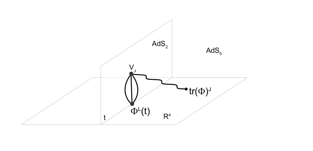
Refer to caption
Figure 6: Depiction of the leading order contribution to the bulk-defect correlator at strong coupling.

It is not difficult to see that only VJAdS5superscriptsubscript𝑉𝐽subscriptAdS5V_{J}^{{\rm AdS}_{5}} contributes to this order, because expansion of VJS5superscriptsubscript𝑉𝐽subscriptS5V_{J}^{{\rm S}_{5}} to L𝐿L-th order in yasuperscript𝑦𝑎y^{a} will always produce terms that vanish upon contraction with the (uy)Lsuperscript𝑢𝑦𝐿(u\cdot y)^{L} boundary insertion, due to u2=0superscript𝑢20u^{2}=0. Then, the relevant part of the vertex operator expanded to L𝐿L-th power in y𝑦y is found to be, after a bit of algebra:

VJ(x;U)=4J𝒞Jλπdtdss2[(x)2(ss2+(tt)2+(x)2)J+2(Uy)L(U3)JLJ!L!(JL)!+]subscript𝑉𝐽superscript𝑥𝑈4𝐽subscript𝒞𝐽𝜆𝜋𝑑𝑡𝑑𝑠superscript𝑠2delimited-[]superscriptsuperscriptsubscript𝑥perpendicular-to2superscript𝑠superscript𝑠2superscript𝑡superscript𝑡2superscriptsuperscriptsubscript𝑥perpendicular-to2𝐽2superscript𝑈𝑦𝐿superscriptsubscript𝑈3𝐽𝐿𝐽𝐿𝐽𝐿V_{J}(x^{\prime};U)=\frac{4J{\cal C}_{J}\sqrt{\lambda}}{\pi}\int\frac{dtds}{s^{2}}\left[(x_{\perp}^{\prime})^{2}\left(\frac{s}{s^{2}+(t-t^{\prime})^{2}+(x_{\perp}^{\prime})^{2}}\right)^{J+2}(U\cdot y)^{L}(U_{3})^{J-L}\frac{J!}{L!(J-L)!}+\ldots\right] (5.15)

Plugging into (5.6) and performing the L!𝐿L! free Wick contractions, we find

(uy(t0))LVJ(x;U)AdS2subscriptdelimited-⟨⟩superscript𝑢𝑦subscript𝑡0𝐿subscript𝑉𝐽superscript𝑥𝑈subscriptAdS2\displaystyle\langle(u\cdot y(t_{0}))^{L}V_{J}(x^{\prime};U)\,\rangle_{{\rm AdS}_{2}} =4J𝒞Jλπ(uU)L(U3)JLJ!(JL)!(x)2×\displaystyle=\frac{4J{\cal C}_{J}\sqrt{\lambda}}{\pi}(u\cdot U)^{L}(U_{3})^{J-L}\frac{J!}{(J-L)!}(x_{\perp}^{\prime})^{2}\times (5.16)
×AdS2dtdss2(ss2+(tt)2+(x)2)J+2(sπ(s2+(tt0)2))L\displaystyle\times\int_{{\rm AdS}_{2}}\frac{dtds}{s^{2}}\left(\frac{s}{s^{2}+(t-t^{\prime})^{2}+(x_{\perp}^{\prime})^{2}}\right)^{J+2}\left(\frac{s}{\pi(s^{2}+(t-t_{0})^{2})}\right)^{L}

Evaluating the integral, for instance by introducing Schwinger parameters, yields

AdS2dtdss2(ss2+(tt)2+(x)2)J+2(ss2+(tt0)2)L=subscriptsubscriptAdS2𝑑𝑡𝑑𝑠superscript𝑠2superscript𝑠superscript𝑠2superscript𝑡superscript𝑡2superscriptsuperscriptsubscript𝑥perpendicular-to2𝐽2superscript𝑠superscript𝑠2superscript𝑡subscript𝑡02𝐿absent\displaystyle\int_{{\rm AdS}_{2}}\frac{dtds}{s^{2}}\left(\frac{s}{s^{2}+(t-t^{\prime})^{2}+(x_{\perp}^{\prime})^{2}}\right)^{J+2}\left(\frac{s}{s^{2}+(t-t_{0})^{2}}\right)^{L}= (5.17)
πΓ(12(JL+2))Γ(12(J+L+1))2Γ(J+2)(x)LJ2((t0t)2+(x)2)L.𝜋Γ12𝐽𝐿2Γ12𝐽𝐿12Γ𝐽2superscriptsuperscriptsubscript𝑥perpendicular-to𝐿𝐽2superscriptsuperscriptsubscript𝑡0superscript𝑡2superscriptsuperscriptsubscript𝑥perpendicular-to2𝐿\displaystyle\frac{\sqrt{\pi}\Gamma\left(\frac{1}{2}(J-L+2)\right)\Gamma\left(\frac{1}{2}(J+L+1)\right)}{2\Gamma(J+2)}\,\frac{(x_{\perp}^{\prime})^{L-J-2}}{\left((t_{0}-t^{\prime})^{2}+(x_{\perp}^{\prime})^{2}\right)^{L}}\,.

Putting everything together, we arrive at the final result

(uy(t0))LVJ(x;U)AdS2=2J2+L1JλΓ(12(J+L+1))NcπLΓ(L+1)Γ(12(JL+1))(uU)L(U3)JL(x)JL((t0t)2+(x)2)Lsubscriptdelimited-⟨⟩superscript𝑢𝑦subscript𝑡0𝐿subscript𝑉𝐽superscript𝑥𝑈subscriptAdS2superscript2𝐽2𝐿1𝐽𝜆Γ12𝐽𝐿1subscript𝑁𝑐superscript𝜋𝐿Γ𝐿1Γ12𝐽𝐿1superscript𝑢𝑈𝐿superscriptsubscript𝑈3𝐽𝐿superscriptsuperscriptsubscript𝑥perpendicular-to𝐽𝐿superscriptsuperscriptsubscript𝑡0superscript𝑡2superscriptsuperscriptsubscript𝑥perpendicular-to2𝐿\langle(u\cdot y(t_{0}))^{L}V_{J}(x^{\prime};U)\,\rangle_{{\rm AdS}_{2}}=\frac{2^{-\frac{J}{2}+L-1}\sqrt{J\lambda}\Gamma\left(\frac{1}{2}(J+L+1)\right)}{N_{c}\pi^{L}\Gamma(L+1)\Gamma\left(\frac{1}{2}(J-L+1)\right)}\frac{(u\cdot U)^{L}(U_{3})^{J-L}}{(x_{\perp}^{\prime})^{J-L}\left((t_{0}-t^{\prime})^{2}+(x_{\perp}^{\prime})^{2}\right)^{L}} (5.18)

Through (5.6) and (2.22), from this we can read off the bulk-defect OPE coefficient cL|Jsubscript𝑐conditional𝐿𝐽c_{L|J} at strong coupling. Now going to the topological configuration on the sphere by using (2.26), we find

𝒲[:Φ~L:]O^Jcircle=(1)L2J21JλΓ(12(J+L+1))NcπLΓ(L+1)Γ(12(JL+1))\langle\!\langle\mathcal{W}[:\!\tilde{\Phi}_{L}\!:\,]\hat{O}_{J}\rangle\!\rangle_{\rm circle}=(-1)^{L}\frac{2^{-\frac{J}{2}-1}\sqrt{J\lambda}\Gamma\left(\frac{1}{2}(J+L+1)\right)}{N_{c}\pi^{L}\Gamma(L+1)\Gamma\left(\frac{1}{2}(J-L+1)\right)} (5.19)

which precisely agrees with the localization prediction (4.43).
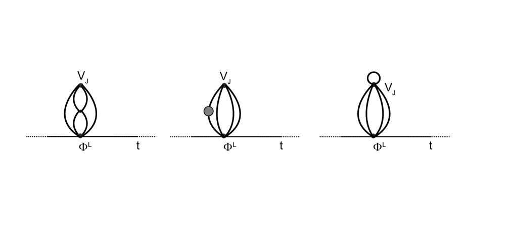
Refer to caption
Figure 7: Diagrams contributing to the next-to-leading order at strong coupling. The first two pictures from the left correspond to bringing down the interaction vertices from the string action while still expanding the vertex operator to L𝐿L-th power in fluctuations. The third diagram arises from expanding the vertex operator to (L+2)𝐿2(L+2)-th order and self-contracting two of the fluctuations.

It would be interesting to compute the subleading strong coupling corrections to this result and compare to localization. To the first subleading order, there are two type of contributions: those that involve the interaction vertices of fluctuations coming from the expansion of the string action, depicted in the first two pictures in Figure 7, and those that involve expanding the vertex operator VJsubscript𝑉𝐽V_{J} to (L+2)𝐿2(L+2)-th order in fluctuations and self-contracting two of those fluctuations, as shown in the third picture in Figure 7. We leave the explicit calculation of these corrections to the future. It is interesting to notice that a precisely analogous structure of subleading corrections also arises in the localization result, see the discussion below eq. (4.38). This suggests that the insertion of BJsubscript𝐵𝐽B_{J} in the contour integral (4.16) essentially plays the role of the vertex operator VJsubscript𝑉𝐽V_{J} on the string theory side.

5.2.1 Two defect insertions and one bulk operator
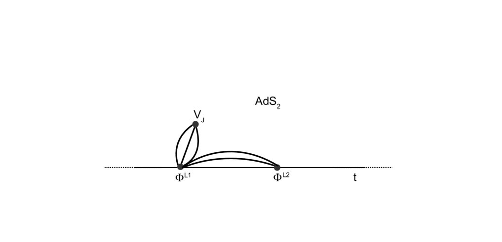
Refer to caption
Figure 8: Leading strong coupling contribution to the correlator of two defect insertions ΦL1superscriptΦsubscript𝐿1\Phi^{L_{1}}, ΦL2superscriptΦsubscript𝐿2\Phi^{L_{2}} and one bulk insertion trΦJtrsuperscriptΦ𝐽{\rm tr}\Phi^{J}.

More general correlators involving several defect and bulk insertions can be computed following a similar procedure. As an example, let us consider the case of two defect insertions and one bulk operator:

𝒲[(u1Φ)L1(t1)(u2Φ)L2(t2)]tr(UΦ)J(x)SYM=(u1y(t1))L1(u2y(t2))L2VJ(x;U)AdS2subscriptdelimited-⟨⟩delimited-⟨⟩𝒲delimited-[]superscriptsubscript𝑢1Φsubscript𝐿1subscript𝑡1superscriptsubscript𝑢2Φsubscript𝐿2subscript𝑡2trsuperscript𝑈Φ𝐽superscript𝑥SYMsubscriptdelimited-⟨⟩superscriptsubscript𝑢1𝑦subscript𝑡1subscript𝐿1superscriptsubscript𝑢2𝑦subscript𝑡2subscript𝐿2subscript𝑉𝐽superscript𝑥𝑈subscriptAdS2\langle\!\langle\mathcal{W}[(u_{1}\cdot\vec{\Phi})^{L_{1}}(t_{1})(u_{2}\cdot\vec{\Phi})^{L_{2}}(t_{2})]\,\,{\rm tr}(U\cdot\vec{\Phi})^{J}(x^{\prime})\rangle\!\rangle_{\rm SYM}=\langle(u_{1}\cdot y(t_{1}))^{L_{1}}(u_{2}\cdot y(t_{2}))^{L_{2}}V_{J}(x^{\prime};U)\,\rangle_{{\rm AdS}_{2}} (5.20)

Let us assume without loss of generality that L1L2subscript𝐿1subscript𝐿2L_{1}\geq L_{2}. The leading order contribution at strong coupling comes from expanding the vertex operator to the smallest possible order in fluctuations, namely to the (L1L2)subscript𝐿1subscript𝐿2(L_{1}-L_{2})-th order, contracting those fluctuations to the boundary insertion (uy)L1superscript𝑢𝑦subscript𝐿1(u\cdot y)^{L_{1}}, and then connecting the remaining fluctuations with L2subscript𝐿2L_{2} “boundary-to-boundary” propagators between the defect insertions. This is depicted in Figure 8. Evaluating this diagram, we find

(u1y(t1))L1(u2y(t2))L2VJ(x;U)AdS2=subscriptdelimited-⟨⟩superscriptsubscript𝑢1𝑦subscript𝑡1subscript𝐿1superscriptsubscript𝑢2𝑦subscript𝑡2subscript𝐿2subscript𝑉𝐽superscript𝑥𝑈subscriptAdS2absent\displaystyle\langle(u_{1}\cdot y(t_{1}))^{L_{1}}(u_{2}\cdot y(t_{2}))^{L_{2}}V_{J}(x^{\prime};U)\,\rangle_{{\rm AdS}_{2}}= (5.21)
=4J𝒞Jλπ(u1U)L1L2(U3)JL1+L2J!L1!(JL1+L2)!(L1L2)!(x)2×\displaystyle=\frac{4J{\cal C}_{J}\sqrt{\lambda}}{\pi}(u_{1}\cdot U)^{L_{1}-L_{2}}(U_{3})^{J-L_{1}+L_{2}}\frac{J!L_{1}!}{(J-L_{1}+L_{2})!(L_{1}-L_{2})!}(x_{\perp}^{\prime})^{2}\times
×(λ2π2u1u2(t1t2)2)L2AdS2dtdss2(ss2+(tt)2+(x)2)J+2(sπ(s2+(tt1)2))L1L2.absentsuperscript𝜆2superscript𝜋2subscript𝑢1subscript𝑢2superscriptsubscript𝑡1subscript𝑡22subscript𝐿2subscriptsubscriptAdS2𝑑𝑡𝑑𝑠superscript𝑠2superscript𝑠superscript𝑠2superscript𝑡superscript𝑡2superscriptsuperscriptsubscript𝑥perpendicular-to2𝐽2superscript𝑠𝜋superscript𝑠2superscript𝑡subscript𝑡12subscript𝐿1subscript𝐿2\displaystyle\times\left(\frac{\sqrt{\lambda}}{2\pi^{2}}\frac{u_{1}\cdot u_{2}}{(t_{1}-t_{2})^{2}}\right)^{L_{2}}\int_{{\rm AdS}_{2}}\frac{dtds}{s^{2}}\left(\frac{s}{s^{2}+(t-t^{\prime})^{2}+(x_{\perp}^{\prime})^{2}}\right)^{J+2}\left(\frac{s}{\pi(s^{2}+(t-t_{1})^{2})}\right)^{L_{1}-L_{2}}\,.

Using the integral (LABEL:KK-integ), the final result is then

(u1y(t1))L1(u2y(t2))L2VJ(x;U)AdS2=cL1,L2|J(u1U)L1L2(U3)JL1+L2(u1u2)L2(x)JL1+L2((t1t)2+(x)2)L1L2(t1t2)2L2subscriptdelimited-⟨⟩superscriptsubscript𝑢1𝑦subscript𝑡1subscript𝐿1superscriptsubscript𝑢2𝑦subscript𝑡2subscript𝐿2subscript𝑉𝐽superscript𝑥𝑈subscriptAdS2subscript𝑐subscript𝐿1conditionalsubscript𝐿2𝐽superscriptsubscript𝑢1𝑈subscript𝐿1subscript𝐿2superscriptsubscript𝑈3𝐽subscript𝐿1subscript𝐿2superscriptsubscript𝑢1subscript𝑢2subscript𝐿2superscriptsuperscriptsubscript𝑥perpendicular-to𝐽subscript𝐿1subscript𝐿2superscriptsuperscriptsubscript𝑡1superscript𝑡2superscriptsuperscriptsubscript𝑥perpendicular-to2subscript𝐿1subscript𝐿2superscriptsubscript𝑡1subscript𝑡22subscript𝐿2\displaystyle\langle(u_{1}\cdot y(t_{1}))^{L_{1}}(u_{2}\cdot y(t_{2}))^{L_{2}}V_{J}(x^{\prime};U)\,\rangle_{{\rm AdS}_{2}}=c_{L_{1},L_{2}|J}\frac{(u_{1}\cdot U)^{L_{1}-L_{2}}(U_{3})^{J-L_{1}+L_{2}}(u_{1}\cdot u_{2})^{L_{2}}}{(x_{\perp}^{\prime})^{J-L_{1}+L_{2}}\left((t_{1}-t^{\prime})^{2}+(x_{\perp}^{\prime})^{2}\right)^{L_{1}-L_{2}}(t_{1}-t_{2})^{2L_{2}}} (5.22)
cL1,L2|J=J2J2+L12L21λ12(L2+1)L1!Γ(12(J+L1L2+1))NcπL1+L2Γ(L1L2+1)Γ(12(JL1+L2+1))subscript𝑐subscript𝐿1conditionalsubscript𝐿2𝐽𝐽superscript2𝐽2subscript𝐿12subscript𝐿21superscript𝜆12subscript𝐿21subscript𝐿1Γ12𝐽subscript𝐿1subscript𝐿21subscript𝑁𝑐superscript𝜋subscript𝐿1subscript𝐿2Γsubscript𝐿1subscript𝐿21Γ12𝐽subscript𝐿1subscript𝐿21\displaystyle c_{L_{1},L_{2}|J}=\frac{\sqrt{J}2^{-\frac{J}{2}+L_{1}-2L_{2}-1}\lambda^{\frac{1}{2}\left(L_{2}+1\right)}L_{1}!\Gamma\left(\frac{1}{2}\left(J+L_{1}-L_{2}+1\right)\right)}{N_{c}\pi^{L_{1}+L_{2}}\Gamma\left(L_{1}-L_{2}+1\right)\Gamma\left(\frac{1}{2}\left(J-L_{1}+L_{2}+1\right)\right)} (5.23)

This gives the correlator on the straight Wilson line. Conformally mapping to the circular loop, and choosing the null polarization vectors corresponding to the topological operators, we obtain the position independent result

𝒲[:Φ~L1::Φ~L2:]O^Jcircle=(1)L1J2J22L21λ12(L2+1)L1!Γ(12(J+L1L2+1))NcπL1+L2Γ(L1L2+1)Γ(12(JL1+L2+1))\langle\!\langle\mathcal{W}[:\!\tilde{\Phi}^{L_{1}}\!:\,:\!\tilde{\Phi}^{L_{2}}\!:\,]\,\,\hat{O}_{J}\rangle\!\rangle_{\rm circle}=(-1)^{L_{1}}\frac{\sqrt{J}2^{-\frac{J}{2}-2L_{2}-1}\lambda^{\frac{1}{2}\left(L_{2}+1\right)}L_{1}!\Gamma\left(\frac{1}{2}\left(J+L_{1}-L_{2}+1\right)\right)}{N_{c}\pi^{L_{1}+L_{2}}\Gamma\left(L_{1}-L_{2}+1\right)\Gamma\left(\frac{1}{2}\left(J-L_{1}+L_{2}+1\right)\right)} (5.24)

This is again in precise agreement with the strong coupling limit of the localization result computed in the Appendix, see eq. (B.13).

6 Non-planar corrections to the defect correlators

As another application of the results in section 3.3, in this section we study the 1/Nc21superscriptsubscript𝑁𝑐21/N_{c}^{2} correction to the correlation functions on the Wilson loop. As will be clear in the analysis below, one has to take into account the mixing with the multi-trace operators in order to reproduce the correct answer. For simplicity, we will focus on the two-point functions,

GL,L=𝒲[:Φ~L::Φ~L:],G_{L,L}=\langle\mathcal{W}[:\!\tilde{\Phi}^{L}\!:\,:\!\tilde{\Phi}^{L}\!:\,]\rangle\,, (6.1)

but the generalization to the higher-point functions is straightforward (although it becomes more complicated).

6.1 Generalities

The nonplanar corrections to GL,Lsubscript𝐺𝐿𝐿G_{L,L} and GL1,L2,L3subscript𝐺subscript𝐿1subscript𝐿2subscript𝐿3G_{L_{1},L_{2},L_{3}} can be studied by using the expansion of the operator determined in section 3.3. For convenience, let us display the formulae again:

:𝒪L:=𝒪L|1/Nc2S1(S2(1)+S2(2))+O(1/Nc2),\displaystyle:\!\mathcal{O}_{L}\!:\,=\left.\typecolon\mathcal{O}_{L}\typecolon\right|_{1/N_{c}^{2}}-S_{1}-(S_{2}^{(1)}+S_{2}^{(2)})+O(1/N_{c}^{2})\,, (6.2)
S1=+j<L0, 1j𝒪𝒪|j𝒪|j𝒪|j𝒪|j,subscript𝑆1subscript𝑗𝐿formulae-sequence01𝑗delimited-⟨⟩subscript𝒪subscript𝒪conditional𝑗delimited-⟨⟩subscript𝒪conditional𝑗subscript𝒪conditional𝑗subscript𝒪conditional𝑗\displaystyle S_{1}=\sum_{\begin{subarray}{c}\ell+j<L\\ 0\leq\ell,\,1\leq j\end{subarray}}\frac{\langle\typecolon\mathcal{O}_{\ell}\typecolon\typecolon\mathcal{O}_{\ell|j}\typecolon\rangle}{\langle\typecolon\mathcal{O}_{\ell|j}\typecolon\typecolon\mathcal{O}_{\ell|j}\typecolon\rangle}\typecolon\mathcal{O}_{\ell|j}\typecolon\,,
S2(1)=+j1+j2<L0, 1j1,j2𝒪L𝒪|j1,j2𝒪|j1,j2𝒪|j1,j2𝒪|j1,j2,superscriptsubscript𝑆21subscriptsubscript𝑗1subscript𝑗2𝐿formulae-sequence01subscript𝑗1subscript𝑗2delimited-⟨⟩subscript𝒪𝐿subscript𝒪conditionalsubscript𝑗1subscript𝑗2delimited-⟨⟩subscript𝒪conditionalsubscript𝑗1subscript𝑗2subscript𝒪conditionalsubscript𝑗1subscript𝑗2subscript𝒪conditionalsubscript𝑗1subscript𝑗2\displaystyle S_{2}^{(1)}=\sum_{\begin{subarray}{c}\ell+j_{1}+j_{2}<L\\ 0\leq\ell,\,1\leq j_{1},j_{2}\end{subarray}}\frac{\langle\typecolon\mathcal{O}_{L}\typecolon\typecolon\mathcal{O}_{\ell|j_{1},j_{2}}\typecolon\rangle}{\langle\typecolon\mathcal{O}_{\ell|j_{1},j_{2}}\typecolon\typecolon\mathcal{O}_{\ell|j_{1},j_{2}}\typecolon\rangle}\typecolon\mathcal{O}_{\ell|j_{1},j_{2}}\typecolon\,,
S2(2)=~<L+j<L𝒪L,𝒪|j𝒪~𝒪|j𝒪|j𝒪|j𝒪~𝒪~𝒪~.superscriptsubscript𝑆22subscript~𝐿subscript𝑗𝐿subscript𝒪𝐿subscript𝒪conditional𝑗delimited-⟨⟩subscript𝒪~subscript𝒪conditional𝑗delimited-⟨⟩subscript𝒪conditional𝑗subscript𝒪conditional𝑗delimited-⟨⟩subscript𝒪~subscript𝒪~subscript𝒪~\displaystyle S_{2}^{(2)}=-\sum_{\tilde{\ell}<L}\,\,\,\sum_{\ell+j<L}\frac{\langle\typecolon\mathcal{O}_{L}\typecolon,\typecolon\mathcal{O}_{\ell|j}\typecolon\rangle\langle\typecolon\mathcal{O}_{\tilde{\ell}}\typecolon\typecolon\mathcal{O}_{\ell|j}\typecolon\rangle}{\langle\typecolon\mathcal{O}_{\ell|j}\typecolon\typecolon\mathcal{O}_{\ell|j}\typecolon\rangle\langle\typecolon\mathcal{O}_{\tilde{\ell}}\typecolon\typecolon\mathcal{O}_{\tilde{\ell}}\typecolon\rangle}\typecolon\mathcal{O}_{\tilde{\ell}}\typecolon\,.

By inspecting these expressions, we conclude that there are four sources of corrections to the correlators at 1/Nc21superscriptsubscript𝑁𝑐21/N_{c}^{2}:

  • The first correction (to be denoted by 𝚏𝚒𝚛𝚜𝚝𝚏𝚒𝚛𝚜𝚝{\tt first}) comes from the terms involving a single S1subscript𝑆1S_{1}. The correction S1subscript𝑆1S_{1} itself is O(1/Nc)𝑂1subscript𝑁𝑐O(1/N_{c}), but since the correlator involving a single 𝒪L|Jsubscript𝒪conditional𝐿𝐽\typecolon\mathcal{O}_{L|J}\typecolon is O(1/Nc)𝑂1subscript𝑁𝑐O(1/N_{c}), in total it gives O(1/Nc2)𝑂1superscriptsubscript𝑁𝑐2O(1/N_{c}^{2}) corrections.

  • The second correction (to be denoted by 𝚜𝚎𝚌𝚘𝚗𝚍𝚜𝚎𝚌𝚘𝚗𝚍{\tt second}) comes from the terms involving two S1subscript𝑆1S_{1}’s. They can contribute at O(1/Nc2)𝑂1superscriptsubscript𝑁𝑐2O(1/N_{c}^{2}) since the correlators involving two identical 𝒪L|Jsubscript𝒪conditional𝐿𝐽\typecolon\mathcal{O}_{L|J}\typecolon can be O(1)𝑂1O(1) (cf. (3.24)).

  • The third correction (to be denoted by 𝚝𝚑𝚒𝚛𝚍𝚝𝚑𝚒𝚛𝚍{\tt third}) comes from the terms involving a single S2(2)superscriptsubscript𝑆22S_{2}^{(2)}. This is by itself O(1/Nc2)𝑂1superscriptsubscript𝑁𝑐2O(1/N_{c}^{2}).

  • In addition to the aforementioned corrections which are induced by the mixing with the multi-trace operators, there are also corrections coming from the 1/Nc21superscriptsubscript𝑁𝑐21/N_{c}^{2} correction to the expectation value of the Wilson loop. Such corrections are already discussed in the previous paper [18], and they can be computed by first expressing the planar result in terms of the planar expectation value of the Wilson loop 𝒲delimited-⟨⟩𝒲\langle\mathcal{W}\rangle, and replacing 𝒲delimited-⟨⟩𝒲\langle\mathcal{W}\rangle with its O(1/Nc2)𝑂1superscriptsubscript𝑁𝑐2O(1/N_{c}^{2}) result given in (2.12). We will denote this correction by adding the subscript |1/Nc2|_{1/N_{c}^{2}} to the planar expression.

Note that the terms involving S2(1)superscriptsubscript𝑆21S_{2}^{(1)} never contribute at this order since the correlator involving 𝒪L|J1,J2subscript𝒪conditional𝐿subscript𝐽1subscript𝐽2\typecolon\mathcal{O}_{L|J_{1},J_{2}}\typecolon is O(1/Nc2)𝑂1superscriptsubscript𝑁𝑐2O(1/N_{c}^{2}), making the whole contribution O(1/Nc4)𝑂1superscriptsubscript𝑁𝑐4O(1/N_{c}^{4}) or higher.

Let us now write down the results explicitly. For this purpose it is convenient to use the large Ncsubscript𝑁𝑐N_{c} factorization and simplify the correlator as242424Here we used O^JO^J=(12)Jdelimited-⟨⟩subscript^𝑂𝐽subscript^𝑂𝐽superscript12𝐽\langle\hat{O}_{J}\hat{O}_{J}\rangle=\left(-\frac{1}{2}\right)^{J}, which follows from our normalization of O^Jsubscript^𝑂𝐽\hat{O}_{J} (2.4).

𝒪L1|J𝒪L2|J𝒪L3𝒪Lndelimited-⟨⟩subscript𝒪conditionalsubscript𝐿1𝐽subscript𝒪conditionalsubscript𝐿2𝐽subscript𝒪subscript𝐿3subscript𝒪subscript𝐿𝑛\displaystyle\langle\typecolon\mathcal{O}_{L_{1}|J}\typecolon\typecolon\mathcal{O}_{L_{2}|J}\typecolon\typecolon\mathcal{O}_{L_{3}}\typecolon\cdots\typecolon\mathcal{O}_{L_{n}}\typecolon\rangle =𝒪L1𝒪L2𝒪L3𝒪LnO^JO^Jabsentdelimited-⟨⟩subscript𝒪subscript𝐿1subscript𝒪subscript𝐿2subscript𝒪subscript𝐿3subscript𝒪subscript𝐿𝑛delimited-⟨⟩subscript^𝑂𝐽subscript^𝑂𝐽\displaystyle=\langle\typecolon\mathcal{O}_{L_{1}}\typecolon\typecolon\mathcal{O}_{L_{2}}\typecolon\typecolon\mathcal{O}_{L_{3}}\typecolon\cdots\typecolon\mathcal{O}_{L_{n}}\typecolon\rangle\langle\hat{O}_{J}\hat{O}_{J}\rangle (6.3)
=(2)J𝒪L1𝒪L2𝒪L3𝒪Ln.absentsuperscript2𝐽delimited-⟨⟩subscript𝒪subscript𝐿1subscript𝒪subscript𝐿2subscript𝒪subscript𝐿3subscript𝒪subscript𝐿𝑛\displaystyle=\left(-2\right)^{-J}\langle\typecolon\mathcal{O}_{L_{1}}\typecolon\typecolon\mathcal{O}_{L_{2}}\typecolon\typecolon\mathcal{O}_{L_{3}}\typecolon\cdots\typecolon\mathcal{O}_{L_{n}}\typecolon\rangle\,.

We can then evaluate the corrections to the two-point functions as follows:

GL,L|𝚏𝚒𝚛𝚜𝚝evaluated-atsubscript𝐺𝐿𝐿𝚏𝚒𝚛𝚜𝚝\displaystyle G_{L,L}|_{\tt first} =2+j<L0, 1j(2)j𝒪L𝒪|j2𝒪𝒪,absent2subscript𝑗𝐿formulae-sequence01𝑗superscript2𝑗superscriptdelimited-⟨⟩subscript𝒪𝐿subscript𝒪conditional𝑗2delimited-⟨⟩subscript𝒪subscript𝒪\displaystyle=-2\sum_{\begin{subarray}{c}\ell+j<L\\ 0\leq\ell,\,1\leq j\end{subarray}}(-2)^{j}\frac{\langle\typecolon\mathcal{O}_{L}\typecolon\typecolon\mathcal{O}_{\ell|j}\typecolon\rangle^{2}}{\langle\typecolon\mathcal{O}_{\ell}\typecolon\typecolon\mathcal{O}_{\ell}\typecolon\rangle}\,, (6.4)
GL,L|𝚜𝚎𝚌𝚘𝚗𝚍evaluated-atsubscript𝐺𝐿𝐿𝚜𝚎𝚌𝚘𝚗𝚍\displaystyle G_{L,L}|_{\tt second} =+j<L0, 1j(2)j𝒪L𝒪|j2𝒪𝒪,absentsubscript𝑗𝐿formulae-sequence01𝑗superscript2𝑗superscriptdelimited-⟨⟩subscript𝒪𝐿subscript𝒪conditional𝑗2delimited-⟨⟩subscript𝒪subscript𝒪\displaystyle=\sum_{\begin{subarray}{c}\ell+j<L\\ 0\leq\ell,\,1\leq j\end{subarray}}(-2)^{j}\frac{\langle\typecolon\mathcal{O}_{L}\typecolon\typecolon\mathcal{O}_{\ell|j}\typecolon\rangle^{2}}{\langle\typecolon\mathcal{O}_{\ell}\typecolon\typecolon\mathcal{O}_{\ell}\typecolon\rangle}\,,
GL,L|𝚝𝚑𝚒𝚛𝚍evaluated-atsubscript𝐺𝐿𝐿𝚝𝚑𝚒𝚛𝚍\displaystyle G_{L,L}|_{\tt third} =0.absent0\displaystyle=0\,.

Note that the third term is zero owing to the restriction on the range of summation L0<Lsubscript𝐿0𝐿L_{0}<L. Summing them up, we obtain the following expression for 1/Nc21superscriptsubscript𝑁𝑐21/N_{c}^{2} corrections to GL,Lsubscript𝐺𝐿𝐿G_{L,L}:

GL,L=𝒪L𝒪L|1/Nc2+j<L0, 1j(2)j𝒪L𝒪|j2𝒪𝒪+O(1/Nc4).subscript𝐺𝐿𝐿evaluated-atdelimited-⟨⟩subscript𝒪𝐿subscript𝒪𝐿1superscriptsubscript𝑁𝑐2subscript𝑗𝐿formulae-sequence01𝑗superscript2𝑗superscriptdelimited-⟨⟩subscript𝒪𝐿subscript𝒪conditional𝑗2delimited-⟨⟩subscript𝒪subscript𝒪𝑂1superscriptsubscript𝑁𝑐4G_{L,L}=\langle\typecolon\mathcal{O}_{L}\typecolon\typecolon\mathcal{O}_{L}\typecolon\rangle|_{1/N_{c}^{2}}-\sum_{\begin{subarray}{c}\ell+j<L\\ 0\leq\ell,\,1\leq j\end{subarray}}(-2)^{j}\frac{\langle\typecolon\mathcal{O}_{L}\typecolon\typecolon\mathcal{O}_{\ell|j}\typecolon\rangle^{2}}{\langle\typecolon\mathcal{O}_{\ell}\typecolon\typecolon\mathcal{O}_{\ell}\typecolon\rangle}+O(1/N_{c}^{4})\,. (6.5)

As mentioned above, the first term 𝒪L𝒪L|1/Nc2evaluated-atdelimited-⟨⟩subscript𝒪𝐿subscript𝒪𝐿1superscriptsubscript𝑁𝑐2\langle\typecolon\mathcal{O}_{L}\typecolon\typecolon\mathcal{O}_{L}\typecolon\rangle|_{1/N_{c}^{2}} can be computed by taking the planar expression and replacing the planar expectation value 𝒲delimited-⟨⟩𝒲\langle\mathcal{W}\rangle with its non-planar counterpart. Similarly, one can also obtain the expressions for the three-point function

GL1,L2,L3=𝒲[:Φ~L1::Φ~L2::Φ~L3:].G_{L_{1},L_{2},L_{3}}=\langle\mathcal{W}[:\!\tilde{\Phi}^{L_{1}}\!:\,:\!\tilde{\Phi}^{L_{2}}\!:\,:\!\tilde{\Phi}^{L_{3}}\!:\,]\rangle\,. (6.6)

The results are summarized in Appendix C.

In the following subsections, we evaluate the expression (6.5) explicitly at weak and strong couplings.

6.2 Weak coupling expansion

Here we evaluate the non-planar corrections for the two-point functions at tree level and compare them with the perturbative answers.

Computation of 𝒪L|1/Nc2evaluated-atsubscript𝒪𝐿1superscriptsubscript𝑁𝑐2\typecolon\mathcal{O}_{L}\typecolon|_{1/N_{c}^{2}}

Before performing the weak-coupling expansion of the correlator, let us first determine the non-planar correction to the operator 𝒪L|1/Nc2evaluated-atsubscript𝒪𝐿1superscriptsubscript𝑁𝑐2\typecolon\mathcal{O}_{L}\typecolon|_{1/N_{c}^{2}}, which comes purely from the non-planar corrections to the expectation value of the Wilson loop 𝒲delimited-⟨⟩𝒲\langle\mathcal{W}\rangle. Note that, as we will see later, such corrections do not contribute to the two-point functions. Nevertheless here we evaluate them explicitly since the results can be used for the computation of higher-point functions.

As shown in the previous paper [18], the corrections coming from the non-planar correction to 𝒲delimited-⟨⟩𝒲\langle\mathcal{W}\rangle can be incorporated by adding the following term252525Note that we already set a=0𝑎0a=0 since we are analyzing the 1/2121/2-BPS loops in this section. to the measure for the integral representation (4.13):

dμ1/Nc2𝑑subscript𝜇1superscriptsubscript𝑁𝑐2\displaystyle d\mu_{1/N_{c}^{2}} =dx2πixe2πg(x+1x)f(2πg(x+1/x)),absent𝑑𝑥2𝜋𝑖𝑥superscript𝑒2𝜋𝑔𝑥1𝑥𝑓2𝜋𝑔𝑥1𝑥\displaystyle=\frac{dx}{2\pi ix}e^{2\pi g(x+\frac{1}{x})}f(2\pi g(x+1/x))\,, (6.7)
f(z)𝑓𝑧\displaystyle f(z) =(2πg)4Nc2z23z+33z4.absentsuperscript2𝜋𝑔4superscriptsubscript𝑁𝑐2superscript𝑧23𝑧33superscript𝑧4\displaystyle=\frac{(2\pi g)^{4}}{N_{c}^{2}}\frac{z^{2}-3z+3}{3z^{4}}\,.

At the leading order in the weak coupling expansion, we obtain

dμ1/Nc2|weak=1Nc2dx2πix1(x+1x)4.evaluated-at𝑑subscript𝜇1superscriptsubscript𝑁𝑐2weak1superscriptsubscript𝑁𝑐2𝑑𝑥2𝜋𝑖𝑥1superscript𝑥1𝑥4\left.d\mu_{1/N_{c}^{2}}\right|_{\rm weak}=\frac{1}{N_{c}^{2}}\frac{dx}{2\pi ix}\frac{1}{(x+\frac{1}{x})^{4}}\,. (6.8)

Because of this correction to the measure, the planar normal-ordered operators 𝒪Lsubscript𝒪𝐿\typecolon\mathcal{O}_{L}\typecolon’s are no longer orthogonal to each other. For instance, the two-point function of 𝒪Lsubscript𝒪𝐿\typecolon\mathcal{O}_{L}\typecolon and 𝒪Msubscript𝒪𝑀\typecolon\mathcal{O}_{M}\typecolon is given by

𝒪L𝒪M|1/Nc2,weak=evaluated-atdelimited-⟨⟩subscript𝒪𝐿subscript𝒪𝑀1superscriptsubscript𝑁𝑐2weakabsent\displaystyle\langle\typecolon\mathcal{O}_{L}\typecolon\typecolon\mathcal{O}_{M}\typecolon\rangle|_{1/N_{c}^{2},\,\,{\rm weak}}= (6.9)
(ig)L+MNc2dx2πix(iLxL+1+iLx(L+1))(iMxM+1+iMx(M+1))(x+1x)6,superscript𝑖𝑔𝐿𝑀superscriptsubscript𝑁𝑐2contour-integral𝑑𝑥2𝜋𝑖𝑥superscript𝑖𝐿superscript𝑥𝐿1superscript𝑖𝐿superscript𝑥𝐿1superscript𝑖𝑀superscript𝑥𝑀1superscript𝑖𝑀superscript𝑥𝑀1superscript𝑥1𝑥6\displaystyle\frac{(-ig)^{L+M}}{N_{c}^{2}}\oint\frac{dx}{2\pi ix}\frac{\left(i^{L}x^{L+1}+i^{-L}x^{-(L+1)}\right)\left(i^{M}x^{M+1}+i^{-M}x^{-(M+1)}\right)}{(x+\frac{1}{x})^{6}}\,,

where we used the weak-coupling expression for the function QLsubscript𝑄𝐿Q_{L} (see also (4.17) and (4.22)):

QL(x)subscript𝑄𝐿𝑥\displaystyle Q_{L}(x) =(ig)L[UL(i(xx1)2)+O(g2)]absentsuperscript𝑖𝑔𝐿delimited-[]subscript𝑈𝐿𝑖𝑥superscript𝑥12𝑂superscript𝑔2\displaystyle=(-ig)^{L}\left[U_{L}\left(\frac{i(x-x^{-1})}{2}\right)+O(g^{2})\right] (6.10)
=(ig)L[iLxL+1+iLx(L+1)x+1x+O(g2)].absentsuperscript𝑖𝑔𝐿delimited-[]superscript𝑖𝐿superscript𝑥𝐿1superscript𝑖𝐿superscript𝑥𝐿1𝑥1𝑥𝑂superscript𝑔2\displaystyle=(-ig)^{L}\left[\frac{i^{L}x^{L+1}+i^{-L}x^{-(L+1)}}{x+\frac{1}{x}}+O(g^{2})\right]\,.

The integral in (6.9) can be computed by using the expansion

1(x+1x)2k=(1)kj=0(1)j(j+k1)!(2k1)!(jk)!x2j(k>0),1superscript𝑥1𝑥2𝑘superscript1𝑘superscriptsubscript𝑗0superscript1𝑗𝑗𝑘12𝑘1𝑗𝑘superscript𝑥2𝑗𝑘subscriptabsent0\frac{1}{\left(x+\frac{1}{x}\right)^{2k}}=(-1)^{k}\sum_{j=0}^{\infty}(-1)^{j}\frac{(j+k-1)!}{(2k-1)!(j-k)!}x^{2j}\qquad(k\in\mathbb{Z}_{>0})\,, (6.11)

as

𝒪L𝒪M|1/Nc2,weak={(ig)L+M120Nc2[(LM2+2)!(LM23)!(L+M2+3)!(L+M22)!](LM: even)0(LM: odd),evaluated-atdelimited-⟨⟩subscript𝒪𝐿subscript𝒪𝑀1superscriptsubscript𝑁𝑐2weakcasessuperscript𝑖𝑔𝐿𝑀120superscriptsubscript𝑁𝑐2delimited-[]𝐿𝑀22𝐿𝑀23𝐿𝑀23𝐿𝑀22:𝐿𝑀 even0:𝐿𝑀 odd\langle\typecolon\mathcal{O}_{L}\typecolon\typecolon\mathcal{O}_{M}\typecolon\rangle|_{1/N_{c}^{2},\,\,{\rm weak}}=\begin{cases}-\frac{(-ig)^{L+M}}{120N_{c}^{2}}\left[\frac{\left(\frac{L-M}{2}+2\right)!}{\left(\frac{L-M}{2}-3\right)!}-\frac{\left(\frac{L+M}{2}+3\right)!}{\left(\frac{L+M}{2}-2\right)!}\right]&\quad(L-M:\text{ even})\\ 0&\quad(L-M:\text{ odd})\end{cases}\,, (6.12)

where we assumed L>M𝐿𝑀L>M. To restore the orthogonality, one simply needs to subtract 𝒪Msubscript𝒪𝑀\typecolon\mathcal{O}_{M}\typecolon from 𝒪Lsubscript𝒪𝐿\typecolon\mathcal{O}_{L}\typecolon as

𝒪L𝒪L0M<L𝒪L𝒪M|1/Nc2,weak𝒪M𝒪M×𝒪M.subscript𝒪𝐿subscript𝒪𝐿subscript0𝑀𝐿evaluated-atdelimited-⟨⟩subscript𝒪𝐿subscript𝒪𝑀1superscriptsubscript𝑁𝑐2weakdelimited-⟨⟩subscript𝒪𝑀subscript𝒪𝑀subscript𝒪𝑀\typecolon\mathcal{O}_{L}\typecolon\quad\to\quad\typecolon\mathcal{O}_{L}\typecolon-\sum_{0\leq M<L}\,\,\frac{\langle\typecolon\mathcal{O}_{L}\typecolon\typecolon\mathcal{O}_{M}\typecolon\rangle|_{1/N_{c}^{2},\,\text{weak}}}{\langle\typecolon\mathcal{O}_{M}\typecolon\typecolon\mathcal{O}_{M}\typecolon\rangle}\times\typecolon\mathcal{O}_{M}\typecolon\,. (6.13)

Subtracting all the operators with smaller lengths, we arrive at the following weak-coupling expression for 𝒪L|1/Nc2evaluated-atsubscript𝒪𝐿1superscriptsubscript𝑁𝑐2\typecolon\mathcal{O}_{L}\typecolon|_{1/N_{c}^{2}}:

𝒪L|1/Nc2,weak=𝒪L+0M<L(ig)LM120Nc2[(LM2+2)!(LM23)!(L+M2+3)!(L+M22)!]𝒪M.evaluated-atsubscript𝒪𝐿1superscriptsubscript𝑁𝑐2weaksubscript𝒪𝐿subscript0𝑀𝐿superscript𝑖𝑔𝐿𝑀120superscriptsubscript𝑁𝑐2delimited-[]𝐿𝑀22𝐿𝑀23𝐿𝑀23𝐿𝑀22subscript𝒪𝑀\typecolon\mathcal{O}_{L}\typecolon|_{1/N_{c}^{2},\,\,{\rm weak}}=\typecolon\mathcal{O}_{L}\typecolon+\sum_{0\leq M<L}\frac{(-ig)^{L-M}}{120N_{c}^{2}}\left[\frac{\left(\frac{L-M}{2}+2\right)!}{\left(\frac{L-M}{2}-3\right)!}-\frac{\left(\frac{L+M}{2}+3\right)!}{\left(\frac{L+M}{2}-2\right)!}\right]\typecolon\mathcal{O}_{M}\typecolon\,. (6.14)

Here we used the weak-coupling expansion of the planar two-point function 𝒪M𝒪M=(g2)M+delimited-⟨⟩subscript𝒪𝑀subscript𝒪𝑀superscriptsuperscript𝑔2𝑀\langle\typecolon\mathcal{O}_{M}\typecolon\typecolon\mathcal{O}_{M}\typecolon\rangle=(-g^{2})^{M}+\cdots.

Two-point functions

Let us now compute the two-point functions at weak coupling by evaluating each term in (6.5). The first term 𝒪L𝒪L1/Nc2subscriptdelimited-⟨⟩subscript𝒪𝐿subscript𝒪𝐿1superscriptsubscript𝑁𝑐2\langle\typecolon\mathcal{O}_{L}\typecolon\typecolon\mathcal{O}_{L}\typecolon\rangle_{1/N_{c}^{2}} can be obtained by setting M=L𝑀𝐿M=L in (6.12) and the result is

𝒪L𝒪L|1/Nc2=(g2)L120Nc2(L+3)!(L2)![1+O(g2)].evaluated-atdelimited-⟨⟩subscript𝒪𝐿subscript𝒪𝐿1superscriptsubscript𝑁𝑐2superscriptsuperscript𝑔2𝐿120superscriptsubscript𝑁𝑐2𝐿3𝐿2delimited-[]1𝑂superscript𝑔2\langle\typecolon\mathcal{O}_{L}\typecolon\typecolon\mathcal{O}_{L}\typecolon\rangle|_{1/N_{c}^{2}}=\frac{(-g^{2})^{L}}{120N_{c}^{2}}\frac{(L+3)!}{(L-2)!}[1+O(g^{2})]\,. (6.15)

Note that the correction to the operator (6.14) does not contribute262626On the other hand, it does contribute for higher-point functions, but we will not perform such computation explicitly in this paper. to the two-point function due to the orthogonality of the planar normal-ordered operators; 𝒪L𝒪M=0delimited-⟨⟩subscript𝒪𝐿subscript𝒪𝑀0\langle\typecolon\mathcal{O}_{L}\typecolon\typecolon\mathcal{O}_{M}\typecolon\rangle=0 for LM𝐿𝑀L\neq M.

The second term is expressed in terms of planar correlators which can be computed by using the integral expression,

𝒪L𝒪|j=2j/2jNc𝑑μBj(x)QL(x)Q(x).delimited-⟨⟩subscript𝒪𝐿subscript𝒪conditional𝑗superscript2𝑗2𝑗subscript𝑁𝑐differential-d𝜇subscript𝐵𝑗𝑥subscript𝑄𝐿𝑥subscript𝑄𝑥\langle\typecolon\mathcal{O}_{L}\typecolon\typecolon\mathcal{O}_{\ell|j}\typecolon\rangle=\frac{2^{-j/2}\sqrt{j}}{N_{c}}\int d\mu\,\,B_{j}(x)Q_{L}(x)Q_{\ell}(x)\,. (6.16)

Using the weak-coupling expansion of each object, we can compute it as272727To compute the integral, we used the expansion (6.11).

𝒪L𝒪|j|weakevaluated-atdelimited-⟨⟩subscript𝒪𝐿subscript𝒪conditional𝑗weak\displaystyle\langle\typecolon\mathcal{O}_{L}\typecolon\typecolon\mathcal{O}_{\ell|j}\typecolon\rangle|_{\rm weak} (6.17)
=(ig)L+2j2jNcdxxj2πix(iLxL+1+iLx(L+1))(ix+1+ix(+1))(x+1x)2absentsuperscript𝑖𝑔𝐿superscript2𝑗2𝑗subscript𝑁𝑐𝑑𝑥superscript𝑥𝑗2𝜋𝑖𝑥superscript𝑖𝐿superscript𝑥𝐿1superscript𝑖𝐿superscript𝑥𝐿1superscript𝑖superscript𝑥1superscript𝑖superscript𝑥1superscript𝑥1𝑥2\displaystyle=\frac{(-ig)^{L+\ell}2^{-\frac{j}{2}}\sqrt{j}}{N_{c}}\int\frac{dx\,\,x^{j}}{2\pi ix}\frac{\left(i^{L}x^{L+1}+i^{-L}x^{-(L+1)}\right)\left(i^{\ell}x^{\ell+1}+i^{-\ell}x^{-(\ell+1)}\right)}{(x+\frac{1}{x})^{2}}
={gL+2j2jNc(1)L++j2(+1)(Lj: even)0(Lj: odd)absentcasessuperscript𝑔𝐿superscript2𝑗2𝑗subscript𝑁𝑐superscript1𝐿𝑗21:𝐿𝑗 even0:𝐿𝑗 odd\displaystyle=\begin{cases}\frac{g^{L+\ell}2^{-\frac{j}{2}}\sqrt{j}}{N_{c}}(-1)^{\frac{L+\ell+j}{2}}(\ell+1)&\quad(L-\ell-j:\text{ even})\\ 0&\quad(L-\ell-j:\text{ odd})\end{cases}

We can thus obtain the following expression for the second term:

+j<L0, 1j(2)j𝒪L𝒪|j2𝒪𝒪subscript𝑗𝐿formulae-sequence01𝑗superscript2𝑗superscriptdelimited-⟨⟩subscript𝒪𝐿subscript𝒪conditional𝑗2delimited-⟨⟩subscript𝒪subscript𝒪\displaystyle-\sum_{\begin{subarray}{c}\ell+j<L\\ 0\leq\ell,\,1\leq j\end{subarray}}(-2)^{j}\frac{\langle\typecolon\mathcal{O}_{L}\typecolon\typecolon\mathcal{O}_{\ell|j}\typecolon\rangle^{2}}{\langle\typecolon\mathcal{O}_{\ell}\typecolon\typecolon\mathcal{O}_{\ell}\typecolon\rangle} =(g2)LNc2+j<L0, 1jj(+1)2(1)Lj+12absentsuperscriptsuperscript𝑔2𝐿superscriptsubscript𝑁𝑐2subscript𝑗𝐿formulae-sequence01𝑗𝑗superscript12superscript1𝐿𝑗12\displaystyle=-\frac{(-g^{2})^{L}}{N_{c}^{2}}\sum_{\begin{subarray}{c}\ell+j<L\\ 0\leq\ell,\,1\leq j\end{subarray}}j(\ell+1)^{2}\frac{(-1)^{L-\ell-j}+1}{2} (6.18)
=(g2)L120Nc2(L+2)!(L3)!.absentsuperscriptsuperscript𝑔2𝐿120superscriptsubscript𝑁𝑐2𝐿2𝐿3\displaystyle=-\frac{(-g^{2})^{L}}{120N_{c}^{2}}\frac{(L+2)!}{(L-3)!}\,.

Adding (6.15) and (6.18) we obtain

GL,L|1/Nc2,weak=124Nc2(L+2)!(L2)!=1Nc2(L+24).evaluated-atsubscript𝐺𝐿𝐿1superscriptsubscript𝑁𝑐2weak124superscriptsubscript𝑁𝑐2𝐿2𝐿21superscriptsubscript𝑁𝑐2𝐿24G_{L,L}|_{1/N_{c}^{2},\,\,{\rm weak}}=\frac{1}{24N_{c}^{2}}\frac{(L+2)!}{(L-2)!}=\frac{1}{N_{c}^{2}}\left(\begin{array}[]{c}L+2\\ 4\end{array}\right)\,. (6.19)
Refer to caption
Figure 9: The general structure of O(1/Nc2)𝑂1superscriptsubscript𝑁𝑐2O(1/N_{c}^{2}) Wick contractions for the two-point functions. The O(1/Nc2)𝑂1superscriptsubscript𝑁𝑐2O(1/N_{c}^{2}) Wick contractions can be obtained by choosing three consecutive segments (whose lengths are denoted by a1,2,3subscript𝑎123a_{1,2,3}) inside the operator and reconnect them as shown in the figure. In order to make the diagram truly non-planar, one further needs to assume that two of the three segments have nonzero lengths. One can count the number of such contractions by counting the number of ways to distribute the four end-points of the segments (denoted by short vertical black lines) inside the operator.

Let us now compare the result (6.19) with the (non-planar) Wick contractions in 𝒩=4𝒩4\mathcal{N}=4 SYM. The general structure of the O(1/Nc2)𝑂1superscriptsubscript𝑁𝑐2O(1/N_{c}^{2}) Wick contractions is depicted in figure 9. As shown there, they are characterized by three non-negative integers a1subscript𝑎1a_{1}, a2subscript𝑎2a_{2} and a3subscript𝑎3a_{3}, which are the lengths of three consecutive segments in the figure. Alternatively, they are specified by the four end-points of these segments. If it were not for any restrictions on the lengths of the segments, the number of ways to specify the four end-points is given by

(𝚌𝚘𝚖𝚋𝚒𝚗𝚊𝚝𝚘𝚛𝚒𝚌𝚜)|naive=(L+44).evaluated-at𝚌𝚘𝚖𝚋𝚒𝚗𝚊𝚝𝚘𝚛𝚒𝚌𝚜naive𝐿44({\tt combinatorics})|_{\rm naive}=\left(\begin{array}[]{c}L+4\\ 4\end{array}\right)\,. (6.20)

This however is not correct since if two of the three lengths a1,2,3subscript𝑎123a_{1,2,3} are zero, the Wick contraction reduces to the planar Wick contraction. To avoid counting such planar contractions, we need to impose the condition a1>0subscript𝑎10a_{1}>0 and a2>0subscript𝑎20a_{2}>0. After imposing this condition, the number of Wick contractions becomes

(𝚌𝚘𝚖𝚋𝚒𝚗𝚊𝚝𝚘𝚛𝚒𝚌𝚜)|correct=(L+24),evaluated-at𝚌𝚘𝚖𝚋𝚒𝚗𝚊𝚝𝚘𝚛𝚒𝚌𝚜correct𝐿24({\tt combinatorics})|_{\rm correct}=\left(\begin{array}[]{c}L+2\\ 4\end{array}\right)\,, (6.21)

which precisely matches the result we computed (6.19).

Before ending this subsection, let us emphasize again that if we did not take into account the mixing with multi-trace operators we would obtain (6.15), which does not match with the result of the Wick contraction. The analysis in this subsection therefore illustrates the importance of the mixing effect and also provides the evidence for our Gram-Schmit analysis.

6.3 Strong coupling expansion

We next compute the non-planar two-point functions at strong coupling.

Computation of 𝒪L|1/Nc2evaluated-atsubscript𝒪𝐿1superscriptsubscript𝑁𝑐2\typecolon\mathcal{O}_{L}\typecolon|_{1/N_{c}^{2}}

As in the previous subsection, let us first determine the correction to the operator 𝒪L|1/Nc2evaluated-atsubscript𝒪𝐿1superscriptsubscript𝑁𝑐2\typecolon\mathcal{O}_{L}\typecolon|_{1/N_{c}^{2}}. For this purpose, we again use the non-planar correction to the measure (6.7). At strong coupling, the integral is dominated by the saddle point x=0𝑥0x=0 and by expanding the measure around the saddle-point in terms of the coordinate used in [18],

x=2πgt2it2πg=1it2πg+O(g1),𝑥2𝜋𝑔superscript𝑡2𝑖𝑡2𝜋𝑔1𝑖𝑡2𝜋𝑔𝑂superscript𝑔1x=\frac{\sqrt{2\pi g-t^{2}}-it}{\sqrt{2\pi g}}=1-\frac{it}{\sqrt{2\pi g}}+O(g^{-1})\,, (6.22)

we obtain

𝑑μ1/Nc2=e4πgg3/26Nc2π2𝑑tet2[166t2+t48πg+O(g2)].contour-integraldifferential-dsubscript𝜇1superscriptsubscript𝑁𝑐2superscript𝑒4𝜋𝑔superscript𝑔326superscriptsubscript𝑁𝑐2𝜋2superscriptsubscriptdifferential-d𝑡superscript𝑒superscript𝑡2delimited-[]166superscript𝑡2superscript𝑡48𝜋𝑔𝑂superscript𝑔2\oint d\mu_{1/N_{c}^{2}}=\frac{e^{4\pi g}g^{3/2}}{6N_{c}^{2}}\sqrt{\frac{\pi}{2}}\int_{-\infty}^{\infty}dt\,\,e^{-t^{2}}\left[1-\frac{6-6t^{2}+t^{4}}{8\pi g}+O(g^{-2})\right]\,. (6.23)

It is convenient to express it in terms of the strong-coupling expansion of the planar measure282828See [18] for derivation.

dμ=e4πg(2π)5/2g3/2dtet2[1t48πg+O(g2)],𝑑𝜇superscript𝑒4𝜋𝑔superscript2𝜋52superscript𝑔32𝑑𝑡superscript𝑒superscript𝑡2delimited-[]1superscript𝑡48𝜋𝑔𝑂superscript𝑔2d\mu=\frac{e^{4\pi g}}{(2\pi)^{5/2}g^{3/2}}dt\,\,e^{-t^{2}}\left[1-\frac{t^{4}}{8\pi g}+O(g^{-2})\right]\,, (6.24)

as

dμ1/Nc2=2g3π33Nc2dμ[1+3(t21)4πg+O(g2)].𝑑subscript𝜇1superscriptsubscript𝑁𝑐22superscript𝑔3superscript𝜋33superscriptsubscript𝑁𝑐2𝑑𝜇delimited-[]13superscript𝑡214𝜋𝑔𝑂superscript𝑔2d\mu_{1/N_{c}^{2}}=\frac{2g^{3}\pi^{3}}{3N_{c}^{2}}d\mu\left[1+\frac{3(t^{2}-1)}{4\pi g}+O(g^{-2})\right]\,. (6.25)

As was computed in the previous paper, the functions QL(x)subscript𝑄𝐿𝑥Q_{L}(x) can be expanded at strong coupling as

QL(x)=1iL(g2π)L2[HL(t)+18πg(L!(2L1)(L2)!HL2(t)+L!(L4)!HL4(t))+O(g2)],subscript𝑄𝐿𝑥1superscript𝑖𝐿superscript𝑔2𝜋𝐿2delimited-[]subscript𝐻𝐿𝑡18𝜋𝑔𝐿2𝐿1𝐿2subscript𝐻𝐿2𝑡𝐿𝐿4subscript𝐻𝐿4𝑡𝑂superscript𝑔2Q_{L}(x)=\frac{1}{i^{L}}\left(\frac{g}{2\pi}\right)^{\frac{L}{2}}\left[H_{L}(t)+\frac{1}{8\pi g}\left(\frac{L!(2L-1)}{(L-2)!}H_{L-2}(t)+\frac{L!}{(L-4)!}H_{L-4}(t)\right)+O(g^{-2})\right]\,,

and are orthogonal to each other under the measure dμ𝑑𝜇d\mu. They are however not orthogonal any more at the non-planar level owing to the correction term in (6.25); 3(t21)/(4πg)3superscript𝑡214𝜋𝑔3(t^{2}-1)/(4\pi g). For instance, the two-point functions of 𝒪Lsubscript𝒪𝐿\typecolon\mathcal{O}_{L}\typecolon and 𝒪Msubscript𝒪𝑀\typecolon\mathcal{O}_{M}\typecolon can be computed as

𝒪L𝒪M|1/Nc2,strong=evaluated-atdelimited-⟨⟩subscript𝒪𝐿subscript𝒪𝑀1superscriptsubscript𝑁𝑐2strongabsent\displaystyle\langle\typecolon\mathcal{O}_{L}\typecolon\typecolon\mathcal{O}_{M}\typecolon\rangle|_{1/N_{c}^{2},\,\,{\rm strong}}= (6.26)
2g3π33Nc2(𝚙𝚕𝚊𝚗𝚊𝚛)+e4πg8Nc21iL+M(g2π)L+M+12𝑑tet2(t21)HL(t)HM(t),2superscript𝑔3superscript𝜋33superscriptsubscript𝑁𝑐2𝚙𝚕𝚊𝚗𝚊𝚛superscript𝑒4𝜋𝑔8superscriptsubscript𝑁𝑐21superscript𝑖𝐿𝑀superscript𝑔2𝜋𝐿𝑀12superscriptsubscriptdifferential-d𝑡superscript𝑒superscript𝑡2superscript𝑡21subscript𝐻𝐿𝑡subscript𝐻𝑀𝑡\displaystyle\frac{2g^{3}\pi^{3}}{3N_{c}^{2}}({\tt planar})+\frac{e^{4\pi g}}{8N_{c}^{2}}\frac{1}{i^{L+M}}\left(\frac{g}{2\pi}\right)^{\frac{L+M+1}{2}}\int_{-\infty}^{\infty}dt\,e^{-t^{2}}(t^{2}-1)H_{L}(t)H_{M}(t)\,,

where (𝚙𝚕𝚊𝚗𝚊𝚛)𝚙𝚕𝚊𝚗𝚊𝚛({\tt planar}) is the planar result computed in [18],

(𝚙𝚕𝚊𝚗𝚊𝚛)=e4πg2(2g)3/2π2(gπ)LL![1332πg(2L2+2L+1)]δL,M.𝚙𝚕𝚊𝚗𝚊𝚛superscript𝑒4𝜋𝑔2superscript2𝑔32superscript𝜋2superscript𝑔𝜋𝐿𝐿delimited-[]1332𝜋𝑔2superscript𝐿22𝐿1subscript𝛿𝐿𝑀({\tt planar})=\frac{e^{4\pi g}}{2(2g)^{3/2}\pi^{2}}\left(-\frac{g}{\pi}\right)^{L}L!\left[1-\frac{3}{32\pi g}(2L^{2}+2L+1)\right]\delta_{L,M}\,. (6.27)

The integral in (6.26) can be computed by using the following properties of the Hermite polynomials:

𝑑tet2HL(t)HM(t)=2LL!πδL,M,superscriptsubscriptdifferential-d𝑡superscript𝑒superscript𝑡2subscript𝐻𝐿𝑡subscript𝐻𝑀𝑡superscript2𝐿𝐿𝜋subscript𝛿𝐿𝑀\displaystyle\int_{-\infty}^{\infty}dt\,e^{-t^{2}}H_{L}(t)H_{M}(t)=2^{L}L!\sqrt{\pi}\delta_{L,M}\,, (6.28)
(t21)HM(t)=HM+2(t)4+2M12HM(t)+M(M1)HM2(t).superscript𝑡21subscript𝐻𝑀𝑡subscript𝐻𝑀2𝑡42𝑀12subscript𝐻𝑀𝑡𝑀𝑀1subscript𝐻𝑀2𝑡\displaystyle(t^{2}-1)H_{M}(t)=\frac{H_{M+2}(t)}{4}+\frac{2M-1}{2}H_{M}(t)+M(M-1)H_{M-2}(t)\,.

The result reads

𝒪L𝒪M|1/Nc2,strong=2g3π33Nc2(𝚙𝚕𝚊𝚗𝚊𝚛)+evaluated-atdelimited-⟨⟩subscript𝒪𝐿subscript𝒪𝑀1superscriptsubscript𝑁𝑐2stronglimit-from2superscript𝑔3superscript𝜋33superscriptsubscript𝑁𝑐2𝚙𝚕𝚊𝚗𝚊𝚛\displaystyle\langle\typecolon\mathcal{O}_{L}\typecolon\typecolon\mathcal{O}_{M}\typecolon\rangle|_{1/N_{c}^{2},\,\,{\rm strong}}=\frac{2g^{3}\pi^{3}}{3N_{c}^{2}}({\tt planar})+ (6.29)
e4πg8Nc2g2(gπ)LL![π2gδL2,M+(2L1)2δL,Mg2π(L+2)(L+1)δL+2,M].superscript𝑒4𝜋𝑔8superscriptsubscript𝑁𝑐2𝑔2superscript𝑔𝜋𝐿𝐿delimited-[]𝜋2𝑔subscript𝛿𝐿2𝑀2𝐿12subscript𝛿𝐿𝑀𝑔2𝜋𝐿2𝐿1subscript𝛿𝐿2𝑀\displaystyle\frac{e^{4\pi g}}{8N_{c}^{2}}\sqrt{\frac{g}{2}}\left(-\frac{g}{\pi}\right)^{L}L!\left[-\frac{\pi}{2g}\delta_{L-2,M}+\frac{(2L-1)}{2}\delta_{L,M}-\frac{g}{2\pi}(L+2)(L+1)\delta_{L+2,M}\right]\,.

As in the weak-coupling analysis, we can restore the orthogonality by performing the following subtraction:

𝒪L|1/Nc2evaluated-atsubscript𝒪𝐿1superscriptsubscript𝑁𝑐2\displaystyle\typecolon\mathcal{O}_{L}\typecolon|_{1/N_{c}^{2}} =𝒪L𝒪L𝒪L2|1/Nc2,strong𝒪L2𝒪L2×𝒪L2absentsubscript𝒪𝐿evaluated-atdelimited-⟨⟩subscript𝒪𝐿subscript𝒪𝐿21superscriptsubscript𝑁𝑐2strongdelimited-⟨⟩subscript𝒪𝐿2subscript𝒪𝐿2subscript𝒪𝐿2\displaystyle=\typecolon\mathcal{O}_{L}\typecolon-\,\,\frac{\langle\typecolon\mathcal{O}_{L}\typecolon\typecolon\mathcal{O}_{L-2}\typecolon\rangle|_{1/N_{c}^{2},\,\,\text{strong}}}{\langle\typecolon\mathcal{O}_{L-2}\typecolon\typecolon\mathcal{O}_{L-2}\typecolon\rangle}\times\typecolon\mathcal{O}_{L-2}\typecolon (6.30)
=𝒪L+π5/2g4Nc2𝒪L2.absentsubscript𝒪𝐿superscript𝜋52𝑔4superscriptsubscript𝑁𝑐2subscript𝒪𝐿2\displaystyle=\typecolon\mathcal{O}_{L}\typecolon+\frac{\pi^{5/2}g}{4N_{c}^{2}}\typecolon\mathcal{O}_{L-2}\typecolon\,.

Here we used the planar two-point functions at strong coupling [18]

𝒪L𝒪L=e4πg2(2g)3/2π2(gπ)LL![1332πg+O(g2)].delimited-⟨⟩subscript𝒪𝐿subscript𝒪𝐿superscript𝑒4𝜋𝑔2superscript2𝑔32superscript𝜋2superscript𝑔𝜋𝐿𝐿delimited-[]1332𝜋𝑔𝑂superscript𝑔2\langle\typecolon\mathcal{O}_{L}\typecolon\typecolon\mathcal{O}_{L}\typecolon\rangle=\frac{e^{4\pi g}}{2(2g)^{3/2}\pi^{2}}\left(-\frac{g}{\pi}\right)^{L}L!\left[1-\frac{3}{32\pi g}+O(g^{-2})\right]\,. (6.31)
Two-point functions

We now proceed to the computation of the non-planar correction to the two-point function. The first term in (6.5) can be computed by setting M=L𝑀𝐿M=L in (6.29),

𝒪L𝒪L|1/Nc2,strong=e4πgg3/2π62Nc2(gπ)LL![13(2L26L+5)32πg].evaluated-atdelimited-⟨⟩subscript𝒪𝐿subscript𝒪𝐿1superscriptsubscript𝑁𝑐2strongsuperscript𝑒4𝜋𝑔superscript𝑔32𝜋62superscriptsubscript𝑁𝑐2superscript𝑔𝜋𝐿𝐿delimited-[]132superscript𝐿26𝐿532𝜋𝑔\langle\typecolon\mathcal{O}_{L}\typecolon\typecolon\mathcal{O}_{L}\typecolon\rangle|_{1/N_{c}^{2},\,{\rm strong}}=\frac{e^{4\pi g}g^{3/2}\pi}{6\sqrt{2}N_{c}^{2}}\left(-\frac{g}{\pi}\right)^{L}L!\left[1-\frac{3(2L^{2}-6L+5)}{32\pi g}\right]\,. (6.32)

On the other hand, the second term, which comes from the mixing with the multi-trace operators, is given in terms of planar correlators involving both the bulk and the defect operators. They can be computed by taking the strong coupling limit of the integral expression (6.16) as was done in section 4.4. However, it turns out that such an integral always scales as

𝒪L𝒪|je4πgg1/2,similar-todelimited-⟨⟩subscript𝒪𝐿subscript𝒪conditional𝑗superscript𝑒4𝜋𝑔superscript𝑔12\langle\typecolon\mathcal{O}_{L}\typecolon\typecolon\mathcal{O}_{\ell|j}\typecolon\rangle\sim e^{4\pi g}g^{\ell-1/2}\,, (6.33)

and once divided by the two-point function it yields

𝒪L𝒪|j2𝒪𝒪e4πgg1.similar-tosuperscriptdelimited-⟨⟩subscript𝒪𝐿subscript𝒪conditional𝑗2delimited-⟨⟩subscript𝒪subscript𝒪superscript𝑒4𝜋𝑔superscript𝑔1\frac{\langle\typecolon\mathcal{O}_{L}\typecolon\typecolon\mathcal{O}_{\ell|j}\typecolon\rangle^{2}}{\langle\typecolon\mathcal{O}_{\ell}\typecolon\typecolon\mathcal{O}_{\ell}\typecolon\rangle}\sim e^{4\pi g}g^{-1}\,. (6.34)

This is always subleading as compared to the first term (6.32). Thus, at the first two orders at strong coupling, one can completely neglect the effect of the mixing with the multi-trace operators and the non-planar correction to the two-point function is simply given by

GL,L|1/Nc2,strong=e4πgg3/2π62Nc2(gπ)LL![13(2L26L+5)32πg].evaluated-atsubscript𝐺𝐿𝐿1superscriptsubscript𝑁𝑐2strongsuperscript𝑒4𝜋𝑔superscript𝑔32𝜋62superscriptsubscript𝑁𝑐2superscript𝑔𝜋𝐿𝐿delimited-[]132superscript𝐿26𝐿532𝜋𝑔G_{L,L}|_{1/N_{c}^{2},\,{\rm strong}}=\frac{e^{4\pi g}g^{3/2}\pi}{6\sqrt{2}N_{c}^{2}}\left(-\frac{g}{\pi}\right)^{L}L!\left[1-\frac{3(2L^{2}-6L+5)}{32\pi g}\right]\,. (6.35)

Using the result for the planar two-point functions (6.31) and the strong-coupling expansion of the Wilson loop expectation value

𝒲=e4πg2(2g)3/2π2[(1332πg+O(g2))+2(πg)33Nc2(11532πg+O(g2))+O(1/Nc4)],delimited-⟨⟩𝒲superscript𝑒4𝜋𝑔2superscript2𝑔32superscript𝜋2delimited-[]1332𝜋𝑔𝑂superscript𝑔22superscript𝜋𝑔33superscriptsubscript𝑁𝑐211532𝜋𝑔𝑂superscript𝑔2𝑂1superscriptsubscript𝑁𝑐4\langle\mathcal{W}\rangle=\frac{e^{4\pi g}}{2(2g)^{3/2}\pi^{2}}\left[\left(1-\frac{3}{32\pi g}+O(g^{-2})\right)+\frac{2(\pi g)^{3}}{3N_{c}^{2}}\left(1-\frac{15}{32\pi g}+O(g^{-2})\right)+O(1/N_{c}^{4})\right]\,,

we obtain the following expression for the normalized correlator:

:𝒪L::𝒪L:=\displaystyle\langle\!\langle:\!\mathcal{O}_{L}\!:\,:\!\mathcal{O}_{L}\!:\,\rangle\!\rangle= (6.36)
(gπ)LL![(13(L+L2)16πg+O(g2))+(πg)2L2Nc2(1+O(g1))+O(1/Nc4)].superscript𝑔𝜋𝐿𝐿delimited-[]13𝐿superscript𝐿216𝜋𝑔𝑂superscript𝑔2superscript𝜋𝑔2𝐿2superscriptsubscript𝑁𝑐21𝑂superscript𝑔1𝑂1superscriptsubscript𝑁𝑐4\displaystyle\left(-\frac{g}{\pi}\right)^{L}L!\left[\left(1-\frac{3(L+L^{2})}{16\pi g}+O(g^{-2})\right)+\frac{(\pi g)^{2}L}{2N_{c}^{2}}\Big{(}1+O(g^{-1})\Big{)}+O(1/N_{c}^{4})\right]\,.

As shown here, the leading non-planar correction at strong coupling is linear in L𝐿L. It would be an interesting future direction to reproduce this result from the string worldsheet by extending the analysis in [14] to the non-planar surface.

6.4 Integral representation and Quantum Spectral Curve

As we already saw in the previous two subsections, the integral representation for the planar correlators is useful for computing the weak and strong coupling expansions of the non-planar two-point functions. At least formally, one can perform the same analysis also at finite ’t Hooft coupling and write down an integral representation of the full non-planar two-point function using the Quantum Spectral Curve.

In particular, it is straightforward to express the first term 𝒪L𝒪L|1/Nc2evaluated-atdelimited-⟨⟩subscript𝒪𝐿subscript𝒪𝐿1superscriptsubscript𝑁𝑐2\langle\typecolon\mathcal{O}_{L}\typecolon\typecolon\mathcal{O}_{L}\typecolon\rangle|_{1/N_{c}^{2}} of (6.5) in terms of an integral since this correction comes from the nonplanar correction to the expectation value of the Wilson loop, which admits an integral representation. Namely, we have292929Note that the function QL(x)subscript𝑄𝐿𝑥Q_{L}(x) used in this expression is the planar Q-functions given in (4.14).

𝒪L𝒪L|1/Nc2=𝑑μ1/Nc2QL(x)QL(x),evaluated-atdelimited-⟨⟩subscript𝒪𝐿subscript𝒪𝐿1superscriptsubscript𝑁𝑐2differential-dsubscript𝜇1superscriptsubscript𝑁𝑐2subscript𝑄𝐿𝑥subscript𝑄𝐿𝑥\langle\typecolon\mathcal{O}_{L}\typecolon\typecolon\mathcal{O}_{L}\typecolon\rangle|_{1/N_{c}^{2}}=\int d\mu_{1/N_{c}^{2}}\,\,Q_{L}(x)Q_{L}(x)\,, (6.37)

where dμ1/Nc2𝑑subscript𝜇1superscriptsubscript𝑁𝑐2d\mu_{1/N_{c}^{2}} is the non-planar correction to the measure given in (6.7).

On the other hand, the second term is given by a sum of ratios of planar correlators. Although the expression might seem quite complicated at first sight, one can simplify it to some extent using the properties of the orthogonal polynomials. To see this, let us first express the summand using the integral expression for the planar correlators:

(2)j𝒪L𝒪|j2𝒪𝒪=superscript2𝑗superscriptdelimited-⟨⟩subscript𝒪𝐿subscript𝒪conditional𝑗2delimited-⟨⟩subscript𝒪subscript𝒪absent\displaystyle(-2)^{j}\frac{\langle\typecolon\mathcal{O}_{L}\typecolon\typecolon\mathcal{O}_{\ell|j}\typecolon\rangle^{2}}{\langle\typecolon\mathcal{O}_{\ell}\typecolon\typecolon\mathcal{O}_{\ell}\typecolon\rangle}= (2)j𝑑μ(x)𝑑μ(y)Bj(x)QL(x)Bj(y)QL(y)Q(x)Q(y)𝑑μQQ.superscript2𝑗differential-d𝜇𝑥differential-d𝜇𝑦subscript𝐵𝑗𝑥subscript𝑄𝐿𝑥subscript𝐵𝑗𝑦subscript𝑄𝐿𝑦subscript𝑄𝑥subscript𝑄𝑦differential-d𝜇subscript𝑄subscript𝑄\displaystyle(-2)^{j}\int d\mu(x)d\mu(y)B_{j}(x)Q_{L}(x)B_{j}(y)Q_{L}(y)\frac{Q_{\ell}(x)Q_{\ell}(y)}{\int d\mu\,Q_{\ell}Q_{\ell}}\,. (6.38)

Since the function QL(x)subscript𝑄𝐿𝑥Q_{L}(x) is an orthogonal polynomial of X=g(xx1)𝑋𝑔𝑥superscript𝑥1X=g(x-x^{-1}), one can perform the summation over \ell using the Christoffel-Darboux theorem (see for instance [53]),

=0Lj1Q(x)Q(y)𝑑μQQ=KLj1(x,y),superscriptsubscript0𝐿𝑗1subscript𝑄𝑥subscript𝑄𝑦differential-d𝜇subscript𝑄subscript𝑄subscript𝐾𝐿𝑗1𝑥𝑦\sum_{\ell=0}^{L-j-1}\frac{Q_{\ell}(x)Q_{\ell}(y)}{\int d\mu\,Q_{\ell}Q_{\ell}}=K_{L-j-1}(x,y)\,, (6.39)

where KL(x,y)subscript𝐾𝐿𝑥𝑦K_{L}(x,y) is the Christoffel-Darboux kernel

KL(x,y)=1𝑑μQLQLQL+1(x)QL(y)QL(x)QL+1(y)g(xy)(1+1xy).subscript𝐾𝐿𝑥𝑦1differential-d𝜇subscript𝑄𝐿subscript𝑄𝐿subscript𝑄𝐿1𝑥subscript𝑄𝐿𝑦subscript𝑄𝐿𝑥subscript𝑄𝐿1𝑦𝑔𝑥𝑦11𝑥𝑦K_{L}(x,y)=\frac{1}{\int d\mu\,Q_{L}Q_{L}}\frac{Q_{L+1}(x)Q_{L}(y)-Q_{L}(x)Q_{L+1}(y)}{g(x-y)(1+\frac{1}{xy})}\,. (6.40)

Using the Christoffel-Darboux kernel, one can express the sum as

+j<L0, 1j(2)j𝒪L𝒪|j2𝒪𝒪=𝑑μ(x)𝑑μ(y)𝒦L(x,y)QL(x)QL(y),subscript𝑗𝐿formulae-sequence01𝑗superscript2𝑗superscriptdelimited-⟨⟩subscript𝒪𝐿subscript𝒪conditional𝑗2delimited-⟨⟩subscript𝒪subscript𝒪differential-d𝜇𝑥differential-d𝜇𝑦subscript𝒦𝐿𝑥𝑦subscript𝑄𝐿𝑥subscript𝑄𝐿𝑦\sum_{\begin{subarray}{c}\ell+j<L\\ 0\leq\ell,\,1\leq j\end{subarray}}(-2)^{j}\frac{\langle\typecolon\mathcal{O}_{L}\typecolon\typecolon\mathcal{O}_{\ell|j}\typecolon\rangle^{2}}{\langle\typecolon\mathcal{O}_{\ell}\typecolon\typecolon\mathcal{O}_{\ell}\typecolon\rangle}=\int d\mu(x)d\mu(y)\mathcal{K}_{L}(x,y)Q_{L}(x)Q_{L}(y)\,, (6.41)

where the kernel 𝒦Lsubscript𝒦𝐿\mathcal{K}_{L} is given by

𝒦L(x,y)=subscript𝒦𝐿𝑥𝑦absent\displaystyle\mathcal{K}_{L}(x,y)= j=0L2(2)Lj1BLj1(x)BLj1(y)Kj(x,y)superscriptsubscript𝑗0𝐿2superscript2𝐿𝑗1subscript𝐵𝐿𝑗1𝑥subscript𝐵𝐿𝑗1𝑦subscript𝐾𝑗𝑥𝑦\displaystyle\sum_{j=0}^{L-2}(-2)^{L-j-1}B_{L-j-1}(x)B_{L-j-1}(y)K_{j}(x,y) (6.42)
=\displaystyle= (4πg)2(2)L1xLyL(1+x2)(1+y2)j=0L2Kj(x,y)(2xy)j.superscript4𝜋𝑔2superscript2𝐿1superscript𝑥𝐿superscript𝑦𝐿1superscript𝑥21superscript𝑦2superscriptsubscript𝑗0𝐿2subscript𝐾𝑗𝑥𝑦superscript2𝑥𝑦𝑗\displaystyle\frac{(4\pi g)^{2}(-2)^{L-1}x^{L}y^{L}}{(1+x^{2})(1+y^{2})}\sum_{j=0}^{L-2}\frac{K_{j}(x,y)}{(-2xy)^{j}}\,.

Note that, although we explicitly performed one of the two sums, the expression (6.41) is slightly formal since the kernel still contains the sum over j𝑗j. It would be interesting to see if we can further simplify the expression.

Now, combining the two terms, we finally get the following integral expression for the non-planar two-point function, which consists of single and double integrals:

GL,L|1/Nc2=𝑑μ1/Nc2QL(x)QL(x)𝑑μ(x)𝑑μ(y)𝒦L(x,y)QL(x)QL(y).evaluated-atsubscript𝐺𝐿𝐿1superscriptsubscript𝑁𝑐2differential-dsubscript𝜇1superscriptsubscript𝑁𝑐2subscript𝑄𝐿𝑥subscript𝑄𝐿𝑥differential-d𝜇𝑥differential-d𝜇𝑦subscript𝒦𝐿𝑥𝑦subscript𝑄𝐿𝑥subscript𝑄𝐿𝑦G_{L,L}|_{1/N_{c}^{2}}=\int d\mu_{1/N_{c}^{2}}Q_{L}(x)Q_{L}(x)-\int d\mu(x)d\mu(y)\mathcal{K}_{L}(x,y)Q_{L}(x)Q_{L}(y)\,. (6.43)

Recently, the integrability-based methods were applied to the non-planar corrections [54, 55, 56, 57]. It would be interesting to compare our formula with such methods and clarify the relation between them.

7 Conclusion

In this paper, we studied the correlation functions of the bulk single-trace operator and the insertions on the Wilson loop using the results from localization. The results are exact and depend nontrivially on the ’t Hooft coupling constant λ𝜆\lambda. At weak coupling, we checked the results against the perturbation theory of 𝒩=4𝒩4\mathcal{N}=4 SYM. At strong coupling, we evaluated the correlation functions of fluctuations of the string worldsheet and the vertex operator, where the former corresponds to the insertion on the Wilson loop and the latter describes the single-trace operator. In both cases, the results are in perfect agreement with what we obtained from localization. We also showed that the results at large Ncsubscript𝑁𝑐N_{c} can be simply expressed in terms of the Q𝑄Q-functions of the quantum spectral curve.

Along the way, we also clarified several aspects of the Gram-Schmidt analysis which were not addressed in the previous paper [18]. Most importantly, we pointed out the necessity of including the multi-trace operators in the operator spectrum for the analysis of non-planar corrections. We then confirmed it by computing the two-point function and comparing it with the perturbation theory.

One possible future direction is to apply our techniques to other theories, such as 𝒩=2𝒩2\mathcal{N}=2 superconformal field theories in four dimensions and ABJM theory in three dimensions. Supersymmetric Wilson loops in these theories were studied from the defect CFT point of view in [58, 59, 60, 61, 62]. In particular, the correlators of a Wilson loop and chiral local operators in the bulk were analyzed recently in [63] using the matrix model and the Gram-Schmidt orthogonalization. It would be interesting to compute more general correlators involving operator insertions on the Wilson loop by generalizing the analysis in this paper.

There are also several other interesting future directions. Firstly, both in this paper and in the previous paper [18], we focused on the Wilson loop in the fundamental representation, and it would be interesting to generalize the analysis to higher-dimensional representations; In particular, when the size of the representation is of order Ncsubscript𝑁𝑐N_{c}, the AdS dual is given by a probe D-brane [64, 65, 66]. One can therefore try to test the results from localization at strong coupling by computing the correlation functions of fluctuations on the D-branes. Work in that direction is in progress [67]. Also interesting would be to consider the representation with O(Nc2)𝑂superscriptsubscript𝑁𝑐2O(N_{c}^{2}) size which corresponds to a nontrivial bubbling geometry [68, 69, 70].

Secondly, it was recently shown that the algebra of operators on the Wilson loop in a certain higher-dimensional representation in 2d2𝑑2d BF theory is isomorphic to 𝔤𝔩(K)𝔤𝔩𝐾\mathfrak{gl}(K) Yangian [71]. Their setup seems to be intimately related to our setup since the BF theory is a zero-coupling limit of 2d2𝑑2d Yang-Mills. It would therefore be interesting to compute the operator algebra in our setup and see if there is an analogous structure.

Thirdly, it would be worth performing a more thorough analysis on the non-planar corrections to the correlators on the Wilson loop and understand their underlying structure. For the expectation value of a single Wilson loop [72] and the correlator of Wilson loops [73], it was recently shown that one can apply the topological recursion [74] and systematically compute the non-planar corrections. It would be interesting if such a method can be generalized to the observables that we studied in this paper.

Yet another direction is to study these correlators using the conformal bootstrap as was initiated in [19, 20]. In supersymmetric theories with exactly marginal directions, one needs to specify the values of the marginal parameters using some additional inputs in order to pin down the theory one wants to bootstrap. The bulk-defect correlators and the defect structure constants which we computed would provide such inputs and can be used as a starting point for the numerical analysis of the defect bootstrap equation [21, 22].

Finally, it would be interesting to try to reproduce the results in this paper by using the integrability machinery. Thanks to the recent developments, we now have integrability-based frameworks to study the correlation functions of single-trace operators [75, 76] and the correlation functions of operators on the Wilson loop [77, 12]. By contrast, the correct framework to analyze the bulk-defect correlators is not known at present time. It would be interesting to try to figure out such a framework by performing explicit computations at weak and strong coupling. Also, the appearance of Q-functions in our final results suggests the utility of the quantum spectral curve for the study of correlation functions. So far there have been three data points (including this paper) [18, 78] which point to such a direction. It would be interesting to connect these dots and try to come up with a fully non-perturbative, integrability-based framework for studying the correlation functions.

Acknowledgement

SK thanks K. Costello, N. Ishtiaque, F. Moosavian, A. Polychronakos, M. Rapcak and Y. Zhou for discussions on related topics. The work of SG is supported in part by the US NSF under Grant No. PHY-1620542. The work of SK is supported by DOE grant number DE-SC0009988.

Appendix A Bulk two-point functions and multi-trace operators

In this appendix, we provide a brief argument on why the multi-trace operators must be included in the defect CFT spectrum using the defect OPE expansion of the bulk two-point function.

In general defect CFTs, the two-point functions of the bulk operators can be expressed as a sum of products of bulk-defect two-point functions,

ObulkObulkOdefectObulkOdefectOdefectObulk.similar-todelimited-⟨⟩subscript𝑂bulksubscript𝑂bulksubscriptsubscript𝑂defectdelimited-⟨⟩subscript𝑂bulksubscript𝑂defectdelimited-⟨⟩subscript𝑂defectsubscript𝑂bulk\langle O_{\rm bulk}O_{\rm bulk}\rangle\sim\sum_{O_{\rm defect}}\langle O_{\rm bulk}O_{\rm defect}\rangle\langle O_{\rm defect}O_{\rm bulk}\rangle\,. (A.1)

This defect OPE expansion applies to physical correlators which depend on the cross ratios. In supersymmetric theories, one can also write down a truncated version of it which is closed in a supersymmetric subsector (called the “micro-bootrstrap equation”) as was shown in [19].

Let us now analyze the consequence of such an expansion on our bulk two-point function. In the large Ncsubscript𝑁𝑐N_{c} limit, the bulk two-point function is given by a sum of the disconnected term (2.14), and the connected term

𝒲O^J1O^J2conn=subscriptdelimited-⟨⟩𝒲subscript^𝑂subscript𝐽1subscript^𝑂subscript𝐽2connabsent\displaystyle\langle\mathcal{W}\hat{O}_{J_{1}}\hat{O}_{J_{2}}\rangle_{\rm conn}= 2(J1+J2)/2J1J2Nc2(2πa2π+a)(J1+J2)/2×\displaystyle\frac{2^{-(J_{1}+J_{2})/2}\sqrt{J_{1}J_{2}}}{N_{c}^{2}}\left(\frac{2\pi-a}{2\pi+a}\right)^{(J_{1}+J_{2})/2}\times (A.2)
[k=1min(J1,J2)(1)k(2π+a2πa)k(J1+J22k)IJ1+J22k(λ)\displaystyle\left[\sum_{k=1}^{{\rm min}(J_{1},J_{2})}(-1)^{k}\left(\frac{2\pi+a}{2\pi-a}\right)^{k}(J_{1}+J_{2}-2k)I_{J_{1}+J_{2}-2k}(\sqrt{\lambda^{\prime}})\right.
+k=1(J1+J2+2k2)IJ1+J2+2k2(λ)]+O(1/Nc4).\displaystyle\left.+\sum_{k=1}^{\infty}(J_{1}+J_{2}+2k-2)I_{J_{1}+J_{2}+2k-2}(\sqrt{\lambda^{\prime}})\right]+O(1/N_{c}^{4})\,.

To interpret them in terms of the defect CFT, one has to divide them by the expectation value of the Wilson loop as was done in section 2.3. After doing so, the disconnected term becomes

O^J1O^J2disc=(12)J1δJ1,J2.subscriptdelimited-⟨⟩delimited-⟨⟩subscript^𝑂subscript𝐽1subscript^𝑂subscript𝐽2discsuperscript12subscript𝐽1subscript𝛿subscript𝐽1subscript𝐽2\langle\!\langle\hat{O}_{J_{1}}\hat{O}_{J_{2}}\rangle\!\rangle_{\rm disc}=\left(-\frac{1}{2}\right)^{J_{1}}\delta_{J_{1},J_{2}}\,. (A.3)

Now, from the fact that this quantity is O(1)𝑂1O(1) (rather than O(1/Nc2)𝑂1superscriptsubscript𝑁𝑐2O(1/N_{c}^{2})), it immediately follows that one has to include operators other than 𝒲[:Φ~L:]\mathcal{W}[:\!\tilde{\Phi}^{L}\!:\,] in the defect CFT spectrum: The bulk-defect two-point functions of 𝒲[:Φ~L:]\mathcal{W}[:\!\tilde{\Phi}^{L}\!:\,] is O(1/Nc)𝑂1subscript𝑁𝑐O(1/N_{c}) as was shown 4 and we would not be able to reproduce the O(1)𝑂1O(1) contribution if we only had these operators. In fact, one can interpret (A.3) as a result of exchanging 𝒪0|J1=𝒲O^J1subscript𝒪conditional0subscript𝐽1𝒲subscript^𝑂subscript𝐽1\mathcal{O}_{0|J_{1}}=\mathcal{W}\hat{O}_{J_{1}}. This explains the necessity of including the “multi-trace” operators in the defect CFT spectrum.

It would be interesting to perform a more thorough analysis of the OPE expansion and the bootstrap equation in the supersymmetric subsector using the results computed in this paper.

Appendix B Correlators with two operator insertions on the Wilson loop

Let us now generalize the computation to the correlation functions of a single bulk operator and two operator insertions on the Wilson loop,

GL1,L2|J𝒲[:Φ~L1::Φ~L2:]O^J.G_{L_{1},L_{2}|J}\equiv\langle\mathcal{W}[:\!\tilde{\Phi}^{L_{1}}\!:\,:\!\tilde{\Phi}^{L_{2}}\!:\,]\,\,\hat{O}_{J}\rangle\,. (B.1)

Using the large Ncsubscript𝑁𝑐N_{c} expansion of :Φ~L1:=:𝒪L1::\!\tilde{\Phi}^{L_{1}}\!:\,=:\!\mathcal{O}_{L_{1}}\!:\, and :Φ~L2:=:𝒪L2::\!\tilde{\Phi}^{L_{2}}\!:\,=:\!\mathcal{O}_{L_{2}}\!:\,, one obtains

GL1,L2|J=subscript𝐺subscript𝐿1conditionalsubscript𝐿2𝐽absent\displaystyle G_{L_{1},L_{2}|J}= 𝒪L1𝒪L2O^J1+J1<L101,1J1𝒪L1𝒪1|J1𝒪1|J1𝒪1|J1𝒪1|J1𝒪L2O^Jdelimited-⟨⟩subscript𝒪subscript𝐿1subscript𝒪subscript𝐿2subscript^𝑂𝐽subscriptsubscript1subscript𝐽1subscript𝐿1formulae-sequence0subscript11subscript𝐽1delimited-⟨⟩subscript𝒪subscript𝐿1subscript𝒪conditionalsubscript1subscript𝐽1delimited-⟨⟩subscript𝒪conditionalsubscript1subscript𝐽1subscript𝒪conditionalsubscript1subscript𝐽1delimited-⟨⟩subscript𝒪conditionalsubscript1subscript𝐽1subscript𝒪subscript𝐿2subscript^𝑂𝐽\displaystyle\langle\typecolon\mathcal{O}_{L_{1}}\typecolon\typecolon\mathcal{O}_{L_{2}}\typecolon\hat{O}_{J}\rangle-\sum_{\begin{subarray}{c}\ell_{1}+J_{1}<L_{1}\\ 0\leq\ell_{1},1\leq J_{1}\end{subarray}}\frac{\langle\typecolon\mathcal{O}_{L_{1}}\typecolon\typecolon\mathcal{O}_{\ell_{1}|J_{1}}\typecolon\rangle}{\langle\typecolon\mathcal{O}_{\ell_{1}|J_{1}}\typecolon\typecolon\mathcal{O}_{\ell_{1}|J_{1}}\typecolon\rangle}\langle\typecolon\mathcal{O}_{\ell_{1}|J_{1}}\typecolon\typecolon\mathcal{O}_{L_{2}}\typecolon\hat{O}_{J}\rangle (B.2)
2+J2<L202,1J2𝒪L2𝒪2|J2𝒪2|J2𝒪2|J2𝒪L1𝒪2|J2O^J+O(1/Nc2).subscriptsubscript2subscript𝐽2subscript𝐿2formulae-sequence0subscript21subscript𝐽2delimited-⟨⟩subscript𝒪subscript𝐿2subscript𝒪conditionalsubscript2subscript𝐽2delimited-⟨⟩subscript𝒪conditionalsubscript2subscript𝐽2subscript𝒪conditionalsubscript2subscript𝐽2delimited-⟨⟩subscript𝒪subscript𝐿1subscript𝒪conditionalsubscript2subscript𝐽2subscript^𝑂𝐽𝑂1superscriptsubscript𝑁𝑐2\displaystyle-\sum_{\begin{subarray}{c}\ell_{2}+J_{2}<L_{2}\\ 0\leq\ell_{2},1\leq J_{2}\end{subarray}}\frac{\langle\typecolon\mathcal{O}_{L_{2}}\typecolon\typecolon\mathcal{O}_{\ell_{2}|J_{2}}\typecolon\rangle}{\langle\typecolon\mathcal{O}_{\ell_{2}|J_{2}}\typecolon\typecolon\mathcal{O}_{\ell_{2}|J_{2}}\typecolon\rangle}\langle\typecolon\mathcal{O}_{L_{1}}\typecolon\typecolon\mathcal{O}_{\ell_{2}|J_{2}}\typecolon\hat{O}_{J}\rangle+O(1/N_{c}^{2})\,.

The second and the third terms are generically suppressed by 1/Nc1subscript𝑁𝑐1/N_{c}. The only cases where these terms are not suppressed are 1. 1=L2subscript1subscript𝐿2\ell_{1}=L_{2} and J1=Jsubscript𝐽1𝐽J_{1}=J, and 2. 2=L1subscript2subscript𝐿1\ell_{2}=L_{1} and J2=Jsubscript𝐽2𝐽J_{2}=J. In the first case, the three-point function 𝒪1|J1𝒪L2O^Jdelimited-⟨⟩subscript𝒪conditionalsubscript1subscript𝐽1subscript𝒪subscript𝐿2subscript^𝑂𝐽\langle\typecolon\mathcal{O}_{\ell_{1}|J_{1}}\typecolon\typecolon\mathcal{O}_{L_{2}}\typecolon\hat{O}_{J}\rangle becomes O(1)𝑂1O(1) and therefore is not suppressed by 1/Nc1subscript𝑁𝑐1/N_{c} while in the second case the same thing happens for 𝒪L1𝒪2|J2O^Jdelimited-⟨⟩subscript𝒪subscript𝐿1subscript𝒪conditionalsubscript2subscript𝐽2subscript^𝑂𝐽\langle\typecolon\mathcal{O}_{L_{1}}\typecolon\typecolon\mathcal{O}_{\ell_{2}|J_{2}}\typecolon\hat{O}_{J}\rangle. Owing to the restriction on the range of the summation over ksubscript𝑘\ell_{k} and Jksubscript𝐽𝑘J_{k} in (B.2), these additional contributions exist only for J<|L1L2|𝐽subscript𝐿1subscript𝐿2J<|L_{1}-L_{2}|.

These additional contributions, when they exist, cancel precisely the first term in (B.2). Therefore we arrive at the following selection rule for the correlator GL1,L2|Jsubscript𝐺subscript𝐿1conditionalsubscript𝐿2𝐽G_{L_{1},L_{2}|J}:

GL1,L2|J={0(J<|L1L2|)𝒪L1𝒪L2O^J(J|L1L2|).subscript𝐺subscript𝐿1conditionalsubscript𝐿2𝐽cases0𝐽subscript𝐿1subscript𝐿2delimited-⟨⟩subscript𝒪subscript𝐿1subscript𝒪subscript𝐿2subscript^𝑂𝐽𝐽subscript𝐿1subscript𝐿2G_{L_{1},L_{2}|J}=\begin{cases}0\qquad&(J<|L_{1}-L_{2}|)\\ \langle\typecolon\mathcal{O}_{L_{1}}\typecolon\typecolon\mathcal{O}_{L_{2}}\typecolon\hat{O}_{J}\rangle\qquad&(J\geq|L_{1}-L_{2}|)\end{cases}\,. (B.3)

In what follows, we compute the leading large Ncsubscript𝑁𝑐N_{c} results at weak and strong couplings303030For simplicity, here we only present the leading weak- and strong-coupling results. using the integral expression (4.16) assuming J|L1L2|𝐽subscript𝐿1subscript𝐿2J\geq|L_{1}-L_{2}|.

B.1 Weak coupling expansion

At the leading order at weak coupling, the function QLisubscript𝑄subscript𝐿𝑖Q_{L_{i}} is given by (see section 4.3)

QLi=(ig)LiULi(cosθ)=(ig)Lisin(Li+1)θsinθ(x=ieiθ),formulae-sequencesubscript𝑄subscript𝐿𝑖superscript𝑖𝑔subscript𝐿𝑖subscript𝑈subscript𝐿𝑖𝜃superscript𝑖𝑔subscript𝐿𝑖subscript𝐿𝑖1𝜃𝜃𝑥𝑖superscript𝑒𝑖𝜃Q_{L_{i}}=(-ig)^{L_{i}}U_{L_{i}}(\cos\theta)=(-ig)^{L_{i}}\frac{\sin(L_{i}+1)\theta}{\sin\theta}\qquad(x=-ie^{i\theta})\,, (B.4)

while the expressions for the measure dμ𝑑𝜇d\mu and BJsubscript𝐵𝐽B_{J} are given in (4.19). Let us now first consider the case where the single-trace operator is sufficiently long, or more precisely the case in which JL1+L2𝐽subscript𝐿1subscript𝐿2J\geq L_{1}+L_{2} is satisfied. In this case, the analysis is similar to the one for GL|Jsubscript𝐺conditional𝐿𝐽G_{L|J} performed in section 4.3: Namely in order to compensate the factor eiJθsuperscript𝑒𝑖𝐽𝜃e^{iJ\theta} contained in BJsubscript𝐵𝐽B_{J}, one has to expand e2gsinθsuperscript𝑒2𝑔𝜃e^{2g\sin\theta} factor up to O(gJL1L2)𝑂superscript𝑔𝐽subscript𝐿1subscript𝐿2O(g^{J-L_{1}-L_{2}}),

dμBJ=dθ2πeiJθiJ(1++gJL1L22JL1L2(2π)JL1L2(JL1L2)!sinJL1L2θ+).𝑑𝜇subscript𝐵𝐽𝑑𝜃2𝜋superscript𝑒𝑖𝐽𝜃superscript𝑖𝐽1superscript𝑔𝐽subscript𝐿1subscript𝐿2superscript2𝐽subscript𝐿1subscript𝐿2superscript2𝜋𝐽subscript𝐿1subscript𝐿2𝐽subscript𝐿1subscript𝐿2superscript𝐽subscript𝐿1subscript𝐿2𝜃d\mu\,\,B_{J}=\frac{d\theta}{2\pi}\frac{e^{iJ\theta}}{i^{J}}\left(1+\cdots+g^{J-L_{1}-L_{2}}\frac{2^{J-L_{1}-L_{2}}(2\pi)^{J-L_{1}-L_{2}}}{(J-L_{1}-L_{2})!}\sin^{J-L_{1}-L_{2}}\theta+\cdots\right)\,. (B.5)

Substituting this term into the integral, we get

GL1,L2|J|weakevaluated-atsubscript𝐺subscript𝐿1conditionalsubscript𝐿2𝐽weak\displaystyle\left.G_{L_{1},L_{2}|J}\right|_{\rm weak} =2J/2JNc(i)J+L1+L2(4π)JL1L2gJ(JL1L2)!dθ2πeiJθsinJL1L2θUL1(cosθ)UL2(cosθ)absentsuperscript2𝐽2𝐽subscript𝑁𝑐superscript𝑖𝐽subscript𝐿1subscript𝐿2superscript4𝜋𝐽subscript𝐿1subscript𝐿2superscript𝑔𝐽𝐽subscript𝐿1subscript𝐿2𝑑𝜃2𝜋superscript𝑒𝑖𝐽𝜃superscript𝐽subscript𝐿1subscript𝐿2𝜃subscript𝑈subscript𝐿1𝜃subscript𝑈subscript𝐿2𝜃\displaystyle=\frac{2^{-J/2}\sqrt{J}}{N_{c}}(-i)^{J+L_{1}+L_{2}}\frac{(4\pi)^{J-L_{1}-L_{2}}g^{J}}{(J-L_{1}-L_{2})!}\int\frac{d\theta}{2\pi}e^{iJ\theta}\sin^{J-L_{1}-L_{2}}\theta\,U_{L_{1}}(\cos\theta)U_{L_{2}}(\cos\theta)\,
=(1)L1+L22J/2JgJNc(2π)JL1L2(JL1L2)!.absentsuperscript1subscript𝐿1subscript𝐿2superscript2𝐽2𝐽superscript𝑔𝐽subscript𝑁𝑐superscript2𝜋𝐽subscript𝐿1subscript𝐿2𝐽subscript𝐿1subscript𝐿2\displaystyle=\frac{(-1)^{L_{1}+L_{2}}2^{-J/2}\sqrt{J}g^{J}}{N_{c}}\frac{(2\pi)^{J-L_{1}-L_{2}}}{(J-L_{1}-L_{2})!}\,. (B.6)

On the other hand, when J𝐽J satisfies

|L1L2|J<L1+L2,L1+L2J:even,|L_{1}-L_{2}|\leq J<L_{1}+L_{2}\,,\qquad L_{1}+L_{2}-J:{\rm even}\,, (B.7)

we do not need to expand e2gsinθsuperscript𝑒2𝑔𝜃e^{2g\sin\theta} to compensate eiJθsuperscript𝑒𝑖𝐽𝜃e^{iJ\theta}. Therefore the integral is given by

GL1,L2|J|weakevaluated-atsubscript𝐺subscript𝐿1conditionalsubscript𝐿2𝐽weak\displaystyle\left.G_{L_{1},L_{2}|J}\right|_{\rm weak} =2J/2JNc(i)J+L1+L2gL1+L2dθ2πeiJθUL1(cosθ)UL2(cosθ)absentsuperscript2𝐽2𝐽subscript𝑁𝑐superscript𝑖𝐽subscript𝐿1subscript𝐿2superscript𝑔subscript𝐿1subscript𝐿2𝑑𝜃2𝜋superscript𝑒𝑖𝐽𝜃subscript𝑈subscript𝐿1𝜃subscript𝑈subscript𝐿2𝜃\displaystyle=\frac{2^{-J/2}\sqrt{J}}{N_{c}}(-i)^{J+L_{1}+L_{2}}g^{L_{1}+L_{2}}\int\frac{d\theta}{2\pi}e^{iJ\theta}\,U_{L_{1}}(\cos\theta)U_{L_{2}}(\cos\theta)\, (B.8)
=2J/2JNc(i)J+L1+L2gL1+L2(L1+L2J+2)2.absentsuperscript2𝐽2𝐽subscript𝑁𝑐superscript𝑖𝐽subscript𝐿1subscript𝐿2superscript𝑔subscript𝐿1subscript𝐿2subscript𝐿1subscript𝐿2𝐽22\displaystyle=\frac{2^{-J/2}\sqrt{J}}{N_{c}}\frac{(-i)^{J+L_{1}+L_{2}}g^{L_{1}+L_{2}}(L_{1}+L_{2}-J+2)}{2}\,.

When J𝐽J satisfies

|L1L2|J<L1+L2,L1+L2J:odd,|L_{1}-L_{2}|\leq J<L_{1}+L_{2}\,,\qquad L_{1}+L_{2}-J:{\rm odd}\,, (B.9)

we need to take the O(g)𝑂𝑔O(g) term in e2gsinθsuperscript𝑒2𝑔𝜃e^{2g\sin\theta}, and the result reads

GL1,L2|J|weakevaluated-atsubscript𝐺subscript𝐿1conditionalsubscript𝐿2𝐽weak\displaystyle\left.G_{L_{1},L_{2}|J}\right|_{\rm weak} =(4π)2J/2JNc(i)J+L1+L2gL1+L2+1dθ2πeiJθsinθUL1(cosθ)UL2(cosθ)absent4𝜋superscript2𝐽2𝐽subscript𝑁𝑐superscript𝑖𝐽subscript𝐿1subscript𝐿2superscript𝑔subscript𝐿1subscript𝐿21𝑑𝜃2𝜋superscript𝑒𝑖𝐽𝜃𝜃subscript𝑈subscript𝐿1𝜃subscript𝑈subscript𝐿2𝜃\displaystyle=\frac{(4\pi)2^{-J/2}\sqrt{J}}{N_{c}}(-i)^{J+L_{1}+L_{2}}g^{L_{1}+L_{2}+1}\int\frac{d\theta}{2\pi}e^{iJ\theta}\sin\theta\,U_{L_{1}}(\cos\theta)U_{L_{2}}(\cos\theta)\,
=π21J/2JNc(i)J+L1+L21gL1+L2+1.absent𝜋superscript21𝐽2𝐽subscript𝑁𝑐superscript𝑖𝐽subscript𝐿1subscript𝐿21superscript𝑔subscript𝐿1subscript𝐿21\displaystyle=\frac{\pi 2^{1-J/2}\sqrt{J}}{N_{c}}(-i)^{J+L_{1}+L_{2}-1}g^{L_{1}+L_{2}+1}\,. (B.10)

In summary, the results at weak coupling are given by the following expressions:

GL1,L2|J=subscript𝐺subscript𝐿1conditionalsubscript𝐿2𝐽absent\displaystyle G_{L_{1},L_{2}|J}=
{0J<|L1L2|2J/2JNc(i)J+L1+L2gL1+L2(L1+L2J+2)2|L1L2|J<L1+L2,L1+L2J:evenπ21J/2JNc(i)J+L1+L21gL1+L2+1|L1L2|J<L1+L2,L1+L2J:odd(1)L1+L22J/2JgJNc(2π)JL1L2(JL1L2)!L1+L2J.\displaystyle\begin{cases}0&J<|L_{1}-L_{2}|\\ \frac{2^{-J/2}\sqrt{J}}{N_{c}}\frac{(-i)^{J+L_{1}+L_{2}}g^{L_{1}+L_{2}}(L_{1}+L_{2}-J+2)}{2}&|L_{1}-L_{2}|\leq J<L_{1}+L_{2}\,,\quad L_{1}+L_{2}-J:{\rm even}\\ \frac{\pi 2^{1-J/2}\sqrt{J}}{N_{c}}(-i)^{J+L_{1}+L_{2}-1}g^{L_{1}+L_{2}+1}&|L_{1}-L_{2}|\leq J<L_{1}+L_{2}\,,\quad L_{1}+L_{2}-J:{\rm odd}\\ \frac{(-1)^{L_{1}+L_{2}}2^{-J/2}\sqrt{J}g^{J}}{N_{c}}\frac{(2\pi)^{J-L_{1}-L_{2}}}{(J-L_{1}-L_{2})!}&L_{1}+L_{2}\leq J\,.\end{cases}

B.2 Strong coupling expansion

We now study the strong coupling limit. As shown in section 4.4, the strong-coupling limit of the relevant quantities is given by

𝑑μ=dte4πget2(2π)5/2g3/2,BJ=2πgk=0(1)kk!(it2πg)kΓ[1+J+k2]Γ[1+Jk2],formulae-sequencecontour-integraldifferential-d𝜇subscriptsuperscript𝑑𝑡superscript𝑒4𝜋𝑔superscript𝑒superscript𝑡2superscript2𝜋52superscript𝑔32subscript𝐵𝐽2𝜋𝑔superscriptsubscript𝑘0superscript1𝑘𝑘superscript𝑖𝑡2𝜋𝑔𝑘Γdelimited-[]1𝐽𝑘2Γdelimited-[]1𝐽𝑘2\displaystyle\oint d\mu=\int^{\infty}_{-\infty}\frac{dt\,e^{4\pi g}e^{-t^{2}}}{(2\pi)^{5/2}g^{3/2}}\,,\quad B_{J}=2\pi g\sum_{k=0}^{\infty}\frac{(-1)^{k}}{k!}\left(it\sqrt{\frac{2}{\pi g}}\right)^{k}\frac{\Gamma[\frac{1+J+k}{2}]}{\Gamma[\frac{1+J-k}{2}]}\,, (B.11)
QL(t)=(i)L(g2π)L/2HL(t).subscript𝑄𝐿𝑡superscript𝑖𝐿superscript𝑔2𝜋𝐿2subscript𝐻𝐿𝑡\displaystyle Q_{L}(t)=(-i)^{L}\left(\frac{g}{2\pi}\right)^{L/2}H_{L}(t)\,.

To get a non-zero answer, one needs to take O(t|L1L2|)𝑂superscript𝑡subscript𝐿1subscript𝐿2O(t^{|L_{1}-L_{2}|}) term in the expansion of BJsubscript𝐵𝐽B_{J}. Then the integral becomes

GL1,L2|J|strong=evaluated-atsubscript𝐺subscript𝐿1conditionalsubscript𝐿2𝐽strongabsent\displaystyle\left.G_{L_{1},L_{2}|J}\right|_{\rm strong}= e4πg2J/2JNc(2π)3/2g1/2|L1L2|!(1π)Lmax(g2)LminΓ[1+J+|L1L2|2]Γ[1+J|L1L2|2]superscript𝑒4𝜋𝑔superscript2𝐽2𝐽subscript𝑁𝑐superscript2𝜋32superscript𝑔12subscript𝐿1subscript𝐿2superscript1𝜋subscript𝐿maxsuperscript𝑔2subscript𝐿minΓdelimited-[]1𝐽subscript𝐿1subscript𝐿22Γdelimited-[]1𝐽subscript𝐿1subscript𝐿22\displaystyle\frac{e^{4\pi g}2^{-J/2}\sqrt{J}}{N_{c}(2\pi)^{3/2}g^{1/2}\,\,|L_{1}-L_{2}|!}\left(-\frac{1}{\pi}\right)^{L_{\rm max}}\left(\frac{g}{2}\right)^{L_{\rm min}}\frac{\Gamma[\frac{1+J+|L_{1}-L_{2}|}{2}]}{\Gamma[\frac{1+J-|L_{1}-L_{2}|}{2}]} (B.12)
×dtet2t|L1L2|HL1(t)HL2(t),\displaystyle\times\int^{\infty}_{-\infty}\,dt\,e^{-t^{2}}t^{|L_{1}-L_{2}|}H_{L_{1}}(t)H_{L_{2}}(t)\,,
=\displaystyle= e4πg21J/2JLmax!Ncπ2g|L1L2|!(1π)LmaxgLminΓ[1+J+|L1L2|2]Γ[1+J|L1L2|2],superscript𝑒4𝜋𝑔superscript21𝐽2𝐽subscript𝐿maxsubscript𝑁𝑐𝜋2𝑔subscript𝐿1subscript𝐿2superscript1𝜋subscript𝐿maxsuperscript𝑔subscript𝐿minΓdelimited-[]1𝐽subscript𝐿1subscript𝐿22Γdelimited-[]1𝐽subscript𝐿1subscript𝐿22\displaystyle\frac{e^{4\pi g}2^{-1-J/2}\sqrt{J}L_{\rm max}!}{N_{c}\pi\sqrt{2g}\,\,|L_{1}-L_{2}|!}\left(-\frac{1}{\pi}\right)^{L_{\rm max}}g^{L_{\rm min}}\frac{\Gamma[\frac{1+J+|L_{1}-L_{2}|}{2}]}{\Gamma[\frac{1+J-|L_{1}-L_{2}|}{2}]}\,,

where Lmaxmax(L1,L2)subscript𝐿maxmaxsubscript𝐿1subscript𝐿2L_{\rm max}\equiv{\rm max}(L_{1},L_{2}) and Lminmin(L1,L2)subscript𝐿minminsubscript𝐿1subscript𝐿2L_{\rm min}\equiv{\rm min}(L_{1},L_{2}).

Let us also consider the normalized correlator by dividing the correlator by the expectation value of the Wilson loop (4.42). We then obtain

GL1,L2|J𝒲|strong=(1)Lmax21J2g1+LminJLmax!πLmax1Nc|L1L2|!Γ[1+J+|L1L2|2]Γ[1+J|L1L2|2].evaluated-atsubscript𝐺subscript𝐿1conditionalsubscript𝐿2𝐽delimited-⟨⟩𝒲strongsuperscript1subscript𝐿maxsuperscript21𝐽2superscript𝑔1subscript𝐿min𝐽subscript𝐿maxsuperscript𝜋subscript𝐿max1subscript𝑁𝑐subscript𝐿1subscript𝐿2Γdelimited-[]1𝐽subscript𝐿1subscript𝐿22Γdelimited-[]1𝐽subscript𝐿1subscript𝐿22\left.\frac{G_{L_{1},L_{2}|J}}{\langle\mathcal{W}\rangle}\right|_{\rm strong}=\frac{(-1)^{L_{\rm max}}2^{1-\frac{J}{2}}g^{1+L_{\rm min}}\sqrt{J}L_{\rm max}!}{\pi^{L_{\rm max}-1}N_{c}\,\,|L_{1}-L_{2}|!}\frac{\Gamma[\frac{1+J+|L_{1}-L_{2}|}{2}]}{\Gamma[\frac{1+J-|L_{1}-L_{2}|}{2}]}\,. (B.13)

This result coincides with the direct perturbative string theory analysis performed in section 5.2.1.

Appendix C Non-planar correction to the three-point functions

Here we show the result for the non-planar correction to the three-point functions on the Wilson loop (6.6). By extending the argument in section 6.1, one can straightforwardly compute the corrections as

GL1,L2,L3|𝚏𝚒𝚛𝚜𝚝=evaluated-atsubscript𝐺subscript𝐿1subscript𝐿2subscript𝐿3𝚏𝚒𝚛𝚜𝚝absent\displaystyle G_{L_{1},L_{2},L_{3}}|_{\tt first}= {s,t,u}={1,2,3}s+js<Ls0s, 1js(2)js𝒪Ls𝒪s|js𝒪s|js𝒪Lt𝒪Lu𝒪s𝒪s,subscript𝑠𝑡𝑢absent123subscriptsubscript𝑠subscript𝑗𝑠subscript𝐿𝑠formulae-sequence0subscript𝑠1subscript𝑗𝑠superscript2subscript𝑗𝑠delimited-⟨⟩subscript𝒪subscript𝐿𝑠subscript𝒪conditionalsubscript𝑠subscript𝑗𝑠delimited-⟨⟩subscript𝒪conditionalsubscript𝑠subscript𝑗𝑠subscript𝒪subscript𝐿𝑡subscript𝒪subscript𝐿𝑢delimited-⟨⟩subscript𝒪subscript𝑠subscript𝒪subscript𝑠\displaystyle-\!\!\!\sum_{\begin{subarray}{c}\{s,t,u\}\\ =\{1,2,3\}\end{subarray}}\sum_{\begin{subarray}{c}\ell_{s}+j_{s}<L_{s}\\ 0\leq\ell_{s},\,1\leq j_{s}\end{subarray}}(-2)^{j_{s}}\frac{\langle\typecolon\mathcal{O}_{L_{s}}\typecolon\typecolon\mathcal{O}_{\ell_{s}|j_{s}}\typecolon\rangle\langle\typecolon\mathcal{O}_{\ell_{s}|j_{s}}\typecolon\typecolon\mathcal{O}_{L_{t}}\typecolon\typecolon\mathcal{O}_{L_{u}}\typecolon\rangle}{\langle\typecolon\mathcal{O}_{\ell_{s}}\typecolon\typecolon\mathcal{O}_{\ell_{s}}\typecolon\rangle}\,, (C.1)
GL1,L2,L3|𝚜𝚎𝚌𝚘𝚗𝚍=evaluated-atsubscript𝐺subscript𝐿1subscript𝐿2subscript𝐿3𝚜𝚎𝚌𝚘𝚗𝚍absent\displaystyle G_{L_{1},L_{2},L_{3}}|_{\tt second}= {s,t,u}={1,2,3}1js+j<Ls0st+j<Lt0t(2)j𝒪Ls𝒪s|j𝒪Lt𝒪t|j𝒪s𝒪s𝒪t𝒪tsubscript𝑠𝑡𝑢absent123subscript1𝑗subscriptsubscript𝑠𝑗subscript𝐿𝑠0subscript𝑠subscriptsubscript𝑡𝑗subscript𝐿𝑡0subscript𝑡superscript2𝑗delimited-⟨⟩subscript𝒪subscript𝐿𝑠subscript𝒪conditionalsubscript𝑠𝑗delimited-⟨⟩subscript𝒪subscript𝐿𝑡subscript𝒪conditionalsubscript𝑡𝑗delimited-⟨⟩subscript𝒪subscript𝑠subscript𝒪subscript𝑠delimited-⟨⟩subscript𝒪subscript𝑡subscript𝒪subscript𝑡\displaystyle\!\!\!\sum_{\begin{subarray}{c}\{s,t,u\}\\ =\{1,2,3\}\end{subarray}}\sum_{1\leq j}\sum_{\begin{subarray}{c}\ell_{s}+j<L_{s}\\ 0\leq\ell_{s}\end{subarray}}\sum_{\begin{subarray}{c}\ell_{t}+j<L_{t}\\ 0\leq\ell_{t}\end{subarray}}(-2)^{j}\frac{\langle\typecolon\mathcal{O}_{L_{s}}\typecolon\typecolon\mathcal{O}_{\ell_{s}|j}\typecolon\rangle\langle\typecolon\mathcal{O}_{L_{t}}\typecolon\typecolon\mathcal{O}_{\ell_{t}|j}\typecolon\rangle}{\langle\typecolon\mathcal{O}_{\ell_{s}}\typecolon\typecolon\mathcal{O}_{\ell_{s}}\typecolon\rangle\langle\typecolon\mathcal{O}_{\ell_{t}}\typecolon\typecolon\mathcal{O}_{\ell_{t}}\typecolon\rangle}
×𝒪s𝒪t𝒪Luabsentdelimited-⟨⟩subscript𝒪subscript𝑠subscript𝒪subscript𝑡subscript𝒪subscript𝐿𝑢\displaystyle\quad\times\langle\typecolon\mathcal{O}_{\ell_{s}}\typecolon\typecolon\mathcal{O}_{\ell_{t}}\typecolon\typecolon\mathcal{O}_{L_{u}}\typecolon\rangle
GL1,L2,L3|𝚝𝚑𝚒𝚛𝚍=evaluated-atsubscript𝐺subscript𝐿1subscript𝐿2subscript𝐿3𝚝𝚑𝚒𝚛𝚍absent\displaystyle G_{L_{1},L_{2},L_{3}}|_{\tt third}= {s,t,u}={1,2,3}~s<Lss+js<Ls(2)js𝒪Ls𝒪s|js𝒪~s𝒪s|js𝒪s𝒪s𝒪~s𝒪~ssubscript𝑠𝑡𝑢absent123subscriptsubscript~𝑠subscript𝐿𝑠subscriptsubscript𝑠subscript𝑗𝑠subscript𝐿𝑠superscript2subscript𝑗𝑠delimited-⟨⟩subscript𝒪subscript𝐿𝑠subscript𝒪conditionalsubscript𝑠subscript𝑗𝑠delimited-⟨⟩subscript𝒪subscript~𝑠subscript𝒪conditionalsubscript𝑠subscript𝑗𝑠delimited-⟨⟩subscript𝒪subscript𝑠subscript𝒪subscript𝑠delimited-⟨⟩subscript𝒪subscript~𝑠subscript𝒪subscript~𝑠\displaystyle\sum_{\begin{subarray}{c}\{s,t,u\}\\ =\{1,2,3\}\end{subarray}}\sum_{\tilde{\ell}_{s}<L_{s}}\,\,\,\sum_{\ell_{s}+j_{s}<L_{s}}(-2)^{j_{s}}\frac{\langle\typecolon\mathcal{O}_{L_{s}}\typecolon\typecolon\mathcal{O}_{\ell_{s}|j_{s}}\typecolon\rangle\langle\typecolon\mathcal{O}_{\tilde{\ell}_{s}}\typecolon\typecolon\mathcal{O}_{\ell_{s}|j_{s}}\typecolon\rangle}{\langle\typecolon\mathcal{O}_{\ell_{s}}\typecolon\typecolon\mathcal{O}_{\ell_{s}}\typecolon\rangle\langle\typecolon\mathcal{O}_{\tilde{\ell}_{s}}\typecolon\typecolon\mathcal{O}_{\tilde{\ell}_{s}}\typecolon\rangle}
×𝒪~s𝒪Lt𝒪Lu.absentdelimited-⟨⟩subscript𝒪subscript~𝑠subscript𝒪subscript𝐿𝑡subscript𝒪subscript𝐿𝑢\displaystyle\quad\times\langle\typecolon\mathcal{O}_{\tilde{\ell}_{s}}\typecolon\typecolon\mathcal{O}_{L_{t}}\typecolon\typecolon\mathcal{O}_{L_{u}}\typecolon\rangle\,.

Here the first sum {s,t,u}={1,2,3}𝑠𝑡𝑢123\{s,t,u\}=\{1,2,3\} denotes the sum over cyclic permutations; namely {s,t,u}={1,2,3},{2,3,1},{3,1,2}𝑠𝑡𝑢123231312\{s,t,u\}=\{1,2,3\},\{2,3,1\},\{3,1,2\}. Thus, in total we obtain the following expression for the correlator:

GL1,L2,L3=subscript𝐺subscript𝐿1subscript𝐿2subscript𝐿3absent\displaystyle G_{L_{1},L_{2},L_{3}}= (C.2)
𝒪L1𝒪L2𝒪L3|1/Nc2+GL1,L2,L3|𝚏𝚒𝚛𝚜𝚝+GL1,L2,L3|𝚜𝚎𝚌𝚘𝚗𝚍+GL1,L2,L3|𝚝𝚑𝚒𝚛𝚍.evaluated-atdelimited-⟨⟩subscript𝒪subscript𝐿1subscript𝒪subscript𝐿2subscript𝒪subscript𝐿31superscriptsubscript𝑁𝑐2evaluated-atsubscript𝐺subscript𝐿1subscript𝐿2subscript𝐿3𝚏𝚒𝚛𝚜𝚝evaluated-atsubscript𝐺subscript𝐿1subscript𝐿2subscript𝐿3𝚜𝚎𝚌𝚘𝚗𝚍evaluated-atsubscript𝐺subscript𝐿1subscript𝐿2subscript𝐿3𝚝𝚑𝚒𝚛𝚍\displaystyle\langle\typecolon\mathcal{O}_{L_{1}}\typecolon\typecolon\mathcal{O}_{L_{2}}\typecolon\typecolon\mathcal{O}_{L_{3}}\typecolon\rangle|_{1/N_{c}^{2}}+G_{L_{1},L_{2},L_{3}}|_{\tt first}+G_{L_{1},L_{2},L_{3}}|_{\tt second}+G_{L_{1},L_{2},L_{3}}|_{\tt third}\,.

Using (C.2), one can also compute the normalized three-point function at O(1/Nc2)𝑂1superscriptsubscript𝑁𝑐2O(1/N_{c}^{2}),

:Φ~L1::Φ~L2::Φ~L3:GL1,L2,L3𝒲.\langle\!\langle:\!\tilde{\Phi}^{L_{1}}\!:\,:\!\tilde{\Phi}^{L_{2}}\!:\,:\!\tilde{\Phi}^{L_{3}}\!:\,\rangle\!\rangle\equiv\frac{G_{L_{1},L_{2},L_{3}}}{\langle\mathcal{W}\rangle}\,. (C.3)

Here we display some of the explicit results for the first two leading orders at weak coupling313131The results are correct up to the order O(1/Nc2)𝑂1superscriptsubscript𝑁𝑐2O(1/N_{c}^{2}).:

:Φ~2::Φ~1::Φ~1:=\displaystyle\langle\!\langle:\!\tilde{\Phi}^{2}\!:\,:\!\tilde{\Phi}^{1}\!:\,:\!\tilde{\Phi}^{1}\!:\,\rangle\!\rangle= g4(1+1Nc2)+2π2g63(1+1Nc2),superscript𝑔411superscriptsubscript𝑁𝑐22superscript𝜋2superscript𝑔6311superscriptsubscript𝑁𝑐2\displaystyle g^{4}\left(1+\frac{1}{N_{c}^{2}}\right)+\frac{2\pi^{2}g^{6}}{3}\left(-1+\frac{1}{N_{c}^{2}}\right)\,, (C.4)
:Φ~2::Φ~2::Φ~2:=\displaystyle\langle\!\langle:\!\tilde{\Phi}^{2}\!:\,:\!\tilde{\Phi}^{2}\!:\,:\!\tilde{\Phi}^{2}\!:\,\rangle\!\rangle= g6(1+7Nc2)+4π2g8Nc2,superscript𝑔617superscriptsubscript𝑁𝑐24superscript𝜋2superscript𝑔8superscriptsubscript𝑁𝑐2\displaystyle-g^{6}\left(1+\frac{7}{N_{c}^{2}}\right)+\frac{4\pi^{2}g^{8}}{N_{c}^{2}}\,,
:Φ~3::Φ~2::Φ~1:=\displaystyle\langle\!\langle:\!\tilde{\Phi}^{3}\!:\,:\!\tilde{\Phi}^{2}\!:\,:\!\tilde{\Phi}^{1}\!:\,\rangle\!\rangle= g6(1+5Nc2)+2π2g83(1+2Nc2),superscript𝑔615superscriptsubscript𝑁𝑐22superscript𝜋2superscript𝑔8312superscriptsubscript𝑁𝑐2\displaystyle-g^{6}\left(1+\frac{5}{N_{c}^{2}}\right)+\frac{2\pi^{2}g^{8}}{3}\left(1+\frac{2}{N_{c}^{2}}\right)\,,
:Φ~3::Φ~3::Φ~2:=\displaystyle\langle\!\langle:\!\tilde{\Phi}^{3}\!:\,:\!\tilde{\Phi}^{3}\!:\,:\!\tilde{\Phi}^{2}\!:\,\rangle\!\rangle= g8(1+22Nc2)+38π2g103Nc2,superscript𝑔8122superscriptsubscript𝑁𝑐238superscript𝜋2superscript𝑔103superscriptsubscript𝑁𝑐2\displaystyle g^{8}\left(1+\frac{22}{N_{c}^{2}}\right)+\frac{38\pi^{2}g^{10}}{3N_{c}^{2}}\,,
:Φ~4::Φ~2::Φ~2:=\displaystyle\langle\!\langle:\!\tilde{\Phi}^{4}\!:\,:\!\tilde{\Phi}^{2}\!:\,:\!\tilde{\Phi}^{2}\!:\,\rangle\!\rangle= g8(1+15Nc2)2π2g83(1+11Nc2),superscript𝑔8115superscriptsubscript𝑁𝑐22superscript𝜋2superscript𝑔83111superscriptsubscript𝑁𝑐2\displaystyle g^{8}\left(1+\frac{15}{N_{c}^{2}}\right)-\frac{2\pi^{2}g^{8}}{3}\left(1+\frac{11}{N_{c}^{2}}\right)\,,
:Φ~4::Φ~3::Φ~1:=\displaystyle\langle\!\langle:\!\tilde{\Phi}^{4}\!:\,:\!\tilde{\Phi}^{3}\!:\,:\!\tilde{\Phi}^{1}\!:\,\rangle\!\rangle= g8(1+15Nc2)2π2g83(1+11Nc2),superscript𝑔8115superscriptsubscript𝑁𝑐22superscript𝜋2superscript𝑔83111superscriptsubscript𝑁𝑐2\displaystyle g^{8}\left(1+\frac{15}{N_{c}^{2}}\right)-\frac{2\pi^{2}g^{8}}{3}\left(1+\frac{11}{N_{c}^{2}}\right)\,,
:Φ~5::Φ~3::Φ~2:=\displaystyle\langle\!\langle:\!\tilde{\Phi}^{5}\!:\,:\!\tilde{\Phi}^{3}\!:\,:\!\tilde{\Phi}^{2}\!:\,\rangle\!\rangle= g10(1+35Nc2)+2π2g123(1+10Nc2),superscript𝑔10135superscriptsubscript𝑁𝑐22superscript𝜋2superscript𝑔123110superscriptsubscript𝑁𝑐2\displaystyle-g^{10}\left(1+\frac{35}{N_{c}^{2}}\right)+\frac{2\pi^{2}g^{12}}{3}\left(1+\frac{10}{N_{c}^{2}}\right)\,,
:Φ~4::Φ~4::Φ~4:=\displaystyle\langle\!\langle:\!\tilde{\Phi}^{4}\!:\,:\!\tilde{\Phi}^{4}\!:\,:\!\tilde{\Phi}^{4}\!:\,\rangle\!\rangle= g12(1+135Nc2)74π2g14Nc2.superscript𝑔121135superscriptsubscript𝑁𝑐274superscript𝜋2superscript𝑔14superscriptsubscript𝑁𝑐2\displaystyle g^{12}\left(1+\frac{135}{N_{c}^{2}}\right)-\frac{74\pi^{2}g^{14}}{N_{c}^{2}}\,.

The leading weak coupling terms are in precise agreement with the direct (planar and non-planar) Wick contractions.

It would be interesting to perform more systematic analysis and also to compute the correlators at strong coupling.

Appendix D Non-planar two-point functions at subleading order

Here we test our results for the non-planar two-point functions (6.5) at the next leading order at weak coupling.

Using the expression (6.5), one can in principle compute the correlators at weak coupling straightforwardly. However, at the next leading order, deriving a formula for general lengths L𝐿L becomes quite complicated in practice. Instead, here we display some explicit results for small-length operators at first two leading orders323232As in (C.4), the results are truncated at O(1/Nc2)𝑂1superscriptsubscript𝑁𝑐2O(1/N_{c}^{2}).:

:Φ~::Φ~:=\displaystyle\langle\!\langle:\!\tilde{\Phi}\!:\,:\!\tilde{\Phi}\!:\,\rangle\!\rangle= g2+2π2g43(11Nc2),superscript𝑔22superscript𝜋2superscript𝑔4311superscriptsubscript𝑁𝑐2\displaystyle-g^{2}+\frac{2\pi^{2}g^{4}}{3}\left(1-\frac{1}{N_{c}^{2}}\right)\,, (D.1)
:Φ~2::Φ~2:=\displaystyle\langle\!\langle:\!\tilde{\Phi}^{2}\!:\,:\!\tilde{\Phi}^{2}\!:\,\rangle\!\rangle= g4(1+1Nc2)2π2g63(11Nc2),superscript𝑔411superscriptsubscript𝑁𝑐22superscript𝜋2superscript𝑔6311superscriptsubscript𝑁𝑐2\displaystyle g^{4}\left(1+\frac{1}{N_{c}^{2}}\right)-\frac{2\pi^{2}g^{6}}{3}\left(1-\frac{1}{N_{c}^{2}}\right)\,, (D.2)
:Φ~3::Φ~3:=\displaystyle\langle\!\langle:\!\tilde{\Phi}^{3}\!:\,:\!\tilde{\Phi}^{3}\!:\,\rangle\!\rangle= g6(1+5Nc2)+2π2g83(1+2Nc2),superscript𝑔615superscriptsubscript𝑁𝑐22superscript𝜋2superscript𝑔8312superscriptsubscript𝑁𝑐2\displaystyle-g^{6}\left(1+\frac{5}{N_{c}^{2}}\right)+\frac{2\pi^{2}g^{8}}{3}\left(1+\frac{2}{N_{c}^{2}}\right)\,, (D.3)
:Φ~4::Φ~4:=\displaystyle\langle\!\langle:\!\tilde{\Phi}^{4}\!:\,:\!\tilde{\Phi}^{4}\!:\,\rangle\!\rangle= g8(1+15Nc2)2π2g103(1+11Nc2),superscript𝑔8115superscriptsubscript𝑁𝑐22superscript𝜋2superscript𝑔103111superscriptsubscript𝑁𝑐2\displaystyle g^{8}\left(1+\frac{15}{N_{c}^{2}}\right)-\frac{2\pi^{2}g^{10}}{3}\left(1+\frac{11}{N_{c}^{2}}\right)\,, (D.4)
:Φ~5::Φ~5:=\displaystyle\langle\!\langle:\!\tilde{\Phi}^{5}\!:\,:\!\tilde{\Phi}^{5}\!:\,\rangle\!\rangle= g10(1+35Nc2)+2π2g123(1+30Nc2),superscript𝑔10135superscriptsubscript𝑁𝑐22superscript𝜋2superscript𝑔123130superscriptsubscript𝑁𝑐2\displaystyle-g^{10}\left(1+\frac{35}{N_{c}^{2}}\right)+\frac{2\pi^{2}g^{12}}{3}\left(1+\frac{30}{N_{c}^{2}}\right)\,, (D.5)
:Φ~6::Φ~6:=\displaystyle\langle\!\langle:\!\tilde{\Phi}^{6}\!:\,:\!\tilde{\Phi}^{6}\!:\,\rangle\!\rangle= g12(1+70Nc2)2π2g143(1+64Nc2),superscript𝑔12170superscriptsubscript𝑁𝑐22superscript𝜋2superscript𝑔143164superscriptsubscript𝑁𝑐2\displaystyle g^{12}\left(1+\frac{70}{N_{c}^{2}}\right)-\frac{2\pi^{2}g^{14}}{3}\left(1+\frac{64}{N_{c}^{2}}\right)\,, (D.6)

More generally, we find the following pattern for the first two orders at weak coupling:

:Φ~L::Φ~L:=(g2)L[(1+(L+24)Nc2)2π2g23(1+(L+24)LNc2)].\langle\!\langle:\!\tilde{\Phi}^{L}\!:\,:\!\tilde{\Phi}^{L}\!:\,\rangle\!\rangle=(-g^{2})^{L}\left[\left(1+\frac{\left(\begin{array}[]{c}L+2\\ 4\end{array}\right)}{N_{c}^{2}}\right)-\frac{2\pi^{2}g^{2}}{3}\left(1+\frac{\left(\begin{array}[]{c}L+2\\ 4\end{array}\right)-L}{N_{c}^{2}}\right)\right]\,. (D.7)

As shown in the previous paper [18] and in section 6.2 of this paper, both the planar results and the tree-level non-planar correction can be derived analytically and they reproduce the results from the perturbation theory. The goal of this appendix is to show that the non-planar correction at one loop, in particular the combinatorial number (L+24)L𝐿24𝐿\left(\begin{array}[]{c}L+2\\ 4\end{array}\right)-L, is also consistent with the perturbation theory.
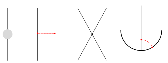
Refer to caption
Figure 10: The diagrams that show up at one loop; the self-energy of a propagator (denoted by a black line), the gluon exchange (denoted by a red dashed line) between two propagators, the scalar quartic interaction and the gluon exchange between a propagator and the Wilson loop (denoted by a thick black curve).
Refer to caption
Figure 11: The gluon exchange diagrams for the planar two-point functions. Here the propagators of the scalar fields are denoted in the double-line notation. The thick black circle denotes the Wilson loop and the red dashed lines are the gluon propagators. Regardless of the lengths of the operators, there are always two such diagrams for the planar two-point functions.

To see this, let us first give a brief summary of the planar results at one loop computed in [12]. At one loop, there are basically four different diagrams (see figure 10) that can contribute to the final answer; the self-energy of a propagator, the gluon exchange between two propagators, the scalar quartic vertex, and the gluon exchange between the Wilson loop and a propagator. Although all the four diagrams are separately divergent, the divergence cancel out when we sum up these diagrams. After the summation, one finds that the finite piece comes solely from the gluon exchanges between the Wilson loop and a propagator. For the two-point functions, there are always two such diagrams (see figure 11) regardless of the lengths of the operators, and the sum of the two gives

(𝚙𝚕𝚊𝚗𝚊𝚛)=2π2g23.𝚙𝚕𝚊𝚗𝚊𝚛2superscript𝜋2superscript𝑔23({\tt planar})=-\frac{2\pi^{2}g^{2}}{3}\,. (D.8)

Multiplying this number to the planar tree-level answer, we reproduce the one-loop planar answer in (D.7).
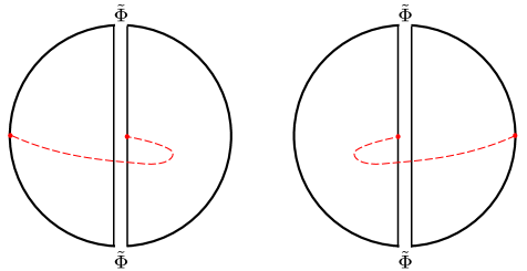
Refer to caption
Figure 12: The non-planar correction to the two-point function of length 111 operators at one loop. As compared to the planar correlator, the gluon is attached to the propagator from the opposite side and this results in an extra minus sign.

We now turn to the non-planar correction. Also at the non-planar level, the same four diagrams show up at one loop and we expect333333We checked this for a few cases. Showing this in general requires more careful analysis which we leave for furture investigation. Instead here we proceed assuming that it is true. that the finite piece comes purely from the gluon exchanges between the Wilson loop and a propagator. The main difference from the planar case is that at the non-planar level the number of such diagrams depends on the length of the operator.

Let us now examine a few cases explicitly. For the length 111 operator, there are two such diagrams as shown in figure 12. As compared to the planar diagrams, the gluon is attached to the propagator from the opposite side and this produces an extra minus sign owing to the anti-symmetry of the structure constant of the gauge group, fabcsubscript𝑓𝑎𝑏𝑐f_{abc}. We therefore conclude that the leading non-planar correction at one loop for the length 1 operator is given by

(𝚗𝚘𝚗𝚙𝚕𝚊𝚗𝚊𝚛)|L=1=(𝚙𝚕𝚊𝚗𝚊𝚛)=+2π2g23.evaluated-at𝚗𝚘𝚗𝚙𝚕𝚊𝚗𝚊𝚛𝐿1𝚙𝚕𝚊𝚗𝚊𝚛2superscript𝜋2superscript𝑔23({\tt nonplanar})|_{L=1}=-({\tt planar})=+\frac{2\pi^{2}g^{2}}{3}\,. (D.9)

Multiplying this number to the planar tree-level answer, we reproduce the result in (D.1).
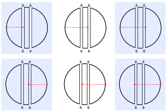
Refer to caption
Figure 13: The non-planar correction to the planar Wick contractions for the length-2 operators. The diagrams depicted in the shaded blue regions come with extra minus signs (as compared to the planar contribution). The result sums up to (𝚙𝚕𝚊𝚗𝚊𝚛)𝚙𝚕𝚊𝚗𝚊𝚛-({\tt planar})
Refer to caption
Figure 14: The gluon exchange diagrams for the non-planar Wick contractions of the length-222 operators. For each propagator, one can attach a gluon from either side and the contributions cancel out with each other.
Refer to caption
Figure 15: Non-planar corrections to the two-point function of the length-333 operators. For each diagram, we showed the gluon exchange diagrams that are not cancelled. (We drew several gluon exchanges in one diagram but they should be understood as separate diagrams.) The first diagram comes from the planar Wick contraction and comes with a minus sign. The last two diagrams are X-shaped diagrams whose contributions add up to zero.

For the length 222 operators, there are two tree-level Wick contractions: The one is planar and the other is non-planar. For the planar Wick contraction, there are six different ways to attach a gluon propagator which makes the full diagram non-planar (see figure 13). Taking into account the minus signs coming from the anti-symmetry of fabcsubscript𝑓𝑎𝑏𝑐f_{abc}, we conclude that they sum up to (𝚙𝚕𝚊𝚗𝚊𝚛)𝚙𝚕𝚊𝚗𝚊𝚛-({\tt planar}). On the other hand, for the non-planar Wick contractions, one can attach a gluon propagator from either side of a scalar propagator and they completely cancel each other (see figure 14). Therefore the final result is given by

(𝚗𝚘𝚗𝚙𝚕𝚊𝚗𝚊𝚛)|L=2=(𝚙𝚕𝚊𝚗𝚊𝚛)=+2π2g23,evaluated-at𝚗𝚘𝚗𝚙𝚕𝚊𝚗𝚊𝚛𝐿2𝚙𝚕𝚊𝚗𝚊𝚛2superscript𝜋2superscript𝑔23({\tt nonplanar})|_{L=2}=-({\tt planar})=+\frac{2\pi^{2}g^{2}}{3}\,, (D.10)

which matches with (D.2).

Let us also analyze the length 333 case. At length 333, there are one planar Wick contraction and five non-planar Wick contractions. For the planar Wick contraction, there are ten different ways to attach a gluon which makes the diagram non-planar. However, most of them cancel each other due to the minus signs coming from fabcsubscript𝑓𝑎𝑏𝑐f_{abc} leaving the two diagrams drawn in figure 15, and we again obtain (𝚙𝚕𝚊𝚗𝚊𝚛)𝚙𝚕𝚊𝚗𝚊𝚛-({\tt planar}) in the end. Now, among the non-planar Wick contractions, two of them have the same topology (“X-shape”) as the non-planar contraction for the length 222 operator and therefore their contributions add up to zero. For the remaining three diagrams, the cancellation is not complete and we are left with the gluon exchanges drawn in figure 15. As a result, each of these three diagrams produces the same contribution as the planar diagram, namely +(𝚙𝚕𝚊𝚗𝚊𝚛)𝚙𝚕𝚊𝚗𝚊𝚛+({\tt planar}). Summing up all, we finally obtain

(𝚗𝚘𝚗𝚙𝚕𝚊𝚗𝚊𝚛)|L=2=(31)(𝚙𝚕𝚊𝚗𝚊𝚛)=+2(𝚙𝚕𝚊𝚗𝚊𝚛)=4π2g23,evaluated-at𝚗𝚘𝚗𝚙𝚕𝚊𝚗𝚊𝚛𝐿231𝚙𝚕𝚊𝚗𝚊𝚛2𝚙𝚕𝚊𝚗𝚊𝚛4superscript𝜋2superscript𝑔23({\tt nonplanar})|_{L=2}=(3-1)({\tt planar})=+2({\tt planar})=-\frac{4\pi^{2}g^{2}}{3}\,, (D.11)

which is again consistent with what we got in (D.2).

By inspecting a few more cases, one can conclude that the planar Wick contraction always produces (𝚙𝚕𝚊𝚗𝚊𝚛)𝚙𝚕𝚊𝚗𝚊𝚛-({\tt planar}) at the non-planar level while the non-planar contraction gives +(𝚙𝚕𝚊𝚗𝚊𝚛)𝚙𝚕𝚊𝚗𝚊𝚛+({\tt planar}) unless the diagram is of the “X-shape” (in which case the contribution is zero). This leads to the following formula for the non-planar correction at one loop:

(𝚗𝚘𝚗𝚙𝚕𝚊𝚗𝚊𝚛)|L=evaluated-at𝚗𝚘𝚗𝚙𝚕𝚊𝚗𝚊𝚛𝐿absent\displaystyle({\tt nonplanar})|_{L}= [(# of non-planar contractions)\displaystyle\left[(\text{\# of non-planar contractions})\right. (D.12)
(# of X-shaped non-planar contractions)1]×(𝚙𝚕𝚊𝚗𝚊𝚛).\displaystyle\left.-(\text{\# of X-shaped non-planar contractions})-1\right]\times({\tt planar})\,.

As computed in section 6.2, the number of non-planar Wick contractions is (L+24)𝐿24\left(\begin{array}[]{c}L+2\\ 4\end{array}\right). On the other hand, the number of X-shaped non-planar contractions is L1𝐿1L-1 since such contractions are specified by a point inside the operator at which we break the operator into two and reconnect. Therefore, we obtain

(𝚗𝚘𝚗𝚙𝚕𝚊𝚗𝚊𝚛)|L=[(L+24)L](𝚙𝚕𝚊𝚗𝚊𝚛)=2π2g23[(L+24)L].evaluated-at𝚗𝚘𝚗𝚙𝚕𝚊𝚗𝚊𝚛𝐿delimited-[]𝐿24𝐿𝚙𝚕𝚊𝚗𝚊𝚛2superscript𝜋2superscript𝑔23delimited-[]𝐿24𝐿({\tt nonplanar})|_{L}=\left[\left(\begin{array}[]{c}L+2\\ 4\end{array}\right)-L\right]({\tt planar})=-\frac{2\pi^{2}g^{2}}{3}\left[\left(\begin{array}[]{c}L+2\\ 4\end{array}\right)-L\right]\,. (D.13)

This matches with the result we computed from localization (D.7).

References