Gravitational waves from binary axionic black holes
Abstract
In a recent paper we have shown that a minimally coupled, self-interacting scalar field of mass can form black holes of mass (in Planck units). If dark matter is composed by axions, they can form miniclusters that for QCD axions have masses below this value. In this work it is shown that for a scenario in which the axion mass depends on the temperature as , minicluster masses above , corresponding to an axion mass of eV, exceed and can collapse into black holes. If a fraction of these black holes is in binary systems, gravitational waves emitted during the inspiral phase could be detected by advanced interferometers like LIGO or VIRGO and by the planned Einstein Telescope. For a detection rate of one event per year, the lower limits on the binary fraction are and for LIGO and Einstein Telescope respectively.
I Introduction
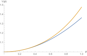
Still hypothetical particles, with masses estimated to be in the range eV up to eV and with a small interaction cross section, axions are up to date the most reliable theoretical explanation for the CP problem of strong interactions CP . In a recent paper EPJC we have shown that scalar fields may, in general, suffer gravitational collapse, producing a central singularity (see also zeldovich ; russos ; russos2 ) and the black hole formed under this process has a mass . This result was derived from an exact solution of the Einstein-Klein-Gordon equations in spherical symmetry, assuming that the scalar field was minimally coupled to gravity. A particular hyperbolic self-interacting potential was adopted, which mimics a free field potential during the first stages of the collapse. For different potentials the collapse (if it occurs) will follow a different evolutionary behavior. Nevertheless, since an initially free field can trigger the collapse, we expect that this happens in general, except for the particular case of a strongly repulsive interaction. In fact, both a potential or the axion potential given in russos3 are less repulsive than the hyperbolic potential adopted in EPJC . This can be shown in Fig. 1 where the axion potential of russos3 is compared with the potential of EPJC for identical initial conditions. On the other hand, Kaup in a seminal paper Kaup solved numerically for the first time the general relativistic Klein-Gordon equation, deriving the eigenstates for spherical symmetry. He concluded that in the free field case there is a maximum mass given by (the so-called Kaup limit), above which the system becomes unstable. Notice that the Kaup limit differs slightly in the numerical factor as compared to the mass mentioned above, probably a consequence of being the result of a series of static equilibrium solutions while the result by EPJC was obtained from a dynamic study of the black hole formation. The inclusion of a self-interaction with potential increases dramatically the maximum mass to (see, for instance, Colpi ). On the other hand, attractive self-interactions lower the maximum mass below the Kaup mass, leading to an instability to axion-nova before the collapse to a black hole russos3 . It should also be emphasised that the maximum mass observed in the diagram “mass versus number of particles”, often called the “critical mass” in the literature, is not necessarily the value above which the system collapses as it was shown by Gleiser Gleiser . This is also true in the case of dense axion stars, which are unstable for masses above this limit and only collapse to black holes for masses still higher russos3 .
On the other hand, axions are good candidates to be cold dark matter particles present in the standard cosmological model cosmology , because they interact very weakly either with baryonic matter or radiation. Axions are produced non-thermally and are the consequence of a spontaneously broken global symmetry, known as a Peccei-Quinn symmetry, which occurs when the temperature of the universe drops below the symmetry breaking scale. If dark matter is composed, at least partially by axions, it is not possible to exclude that mini-axion stars (dubbed miniclusters in the literature) could have been formed from density fluctuations present in the epoch of symmetry breaking. In fact, the phenomenology of the minicluster formation is determined by the cosmic epoch during which the symmetry breaking occurs. Hogan & Rees rees considered a density contrast of the order of the unity and that the typical mass of a mini-axion star corresponds to the mass of all axions inside the horizon at MeV. In this case, the masses of these miniclusters would be about . However, Kolb & Tkachev russos found that oscillations of the axion potential are responsible for non-linear effects controlling the density of mini-axion stars. The mass scale of these objects is fixed as before by the total mass in axions within the horizon but at GeV, when the axion mass is of the order of eV. These effects reduce the mini-axion star mass to about . These masses are below the critical mass expected to trigger the gravitational collapse. Recently, Fairbairn et al. fairbairn revisited the formation of miniclusters, considering different scenarios for the evolution of the axion mass. Here, their results will be used to show that miniclusters of non-QCD axions having masses above , corresponding to an axion mass of eV can collapse and form black holes. In fairbairn , the Press-Schechter formalism was used to compute the mass function of dark halos formed during the hierarchical structure process in which the miniclusters are seeds. Presently, we cannot exclude the possibility that a small fraction of collapsed miniclusters could constitute binary systems formed during successive merger episodes that led to the assembly of dark halos. In this work we will explore this possibility, aiming to constrain the putative fraction of binaries formed during merger events by using the gravitational wave signal emitted during the coalescence of these systems. We will make predictions for the advanced-LIGO pitkin and for the planned Einstein Telescope (ET ) laser interferometers. The paper is organized as follows: in Section II we discuss the critical mass of miniclusters able to collapse, in Section III a simple evolutionary model for the pairs is discussed, in Section IV we give a detailed discussion of the detection of the events and in Section V we present our final considerations.
II Critical Mass
The formation of compact structures constituted by axions or axion-like particles (ALP) is plagued by the absence of an effective cooling mechanism fukugita . In the case of configurations involving scalar fields, different investigations indicate that these systems may relaxe through the emission of bursts of particles seidel ; guzman , a process known as gravitational cooling. Coherent oscillations of the scalar field may also help the relaxation process that leads to the formation of a compact boson star tkachev . Another path to form compact axion-like structures was investigated in shive , where dark mater was assumed to be composed by a non-relativistic bosonic condensate in which the uncertainty principle balances gravity for scales less than the Jeans length. The high resolution cosmological simulations performed with this dark matter model with eV indicate that the resulting large structure is indistinguishable from cold dark matter, but “solitonic” compact structures are generally formed in the core of galaxies.
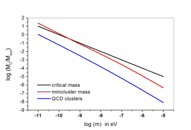
As mentioned before, in the scenario where primordial axion miniclusters are formed, the estimated masses are below the critical value and hence they will not collapse into black holes. The early evolution of axions is determined mainly by two energy scales: the mass and the decay constant . The time at which the axion mass becomes significant is when its Compton wavelength is comparable to the Hubble radius, that is . This mass is a consequence of non-perturbative effects like instantons gross and its evolution with the temperature can be modeled by the relation . For QCD axions , a value which is consistent with lattice simulations. The computed mass of miniclusters by fairbairn as a function of the QCD axion mass is shown in Fig. 2 (blue curve) that is always below the minimum mass (black curve) computed from the relation derived by EPJC .
Higher minicluster masses can be obtained if a more dramatic variation of the axion mass with the temperature is considered. Assuming for instance , minicluster masses up to can be obtained. These large values are not in contradiction with constraints imposed by the Lyman- forest power spectrum fairbairn . The minicluster mass as a function of the axion mass for the case is also shown in Fig. 2 (red curve). Inspection of these plots indicate that, for the temperature evolution scenario with , miniclusters with masses above corresponding to an axion mass of eV are susceptible to undergo the gravitational collapse.
Here it is assumed that a fraction of axion (or ALP) miniclusters of mass constituting dark halos has collapsed and formed black holes. Upper limits from microlensing implies that the maximum contribution of black holes of such a mass to the total dark matter density is about (see freese ), a value that will be adopted in our computations. We assume also that a fraction of these black holes form binary systems, a parameter that will be constrained by the coalescence rate of these systems as we shall see below.
III The evolution of axion black hole binaries
The putative binaries constituted by two black holes of mass have an orbital separation distribution that fixes the rate at which they merge due to energy and angular momentum losses by gravitational radiation. During the inspiral phase of the merger, the wave frequency increases and peaks around the orbital frequency corresponding to a pair separation close to the gravitational radius. Such a characteristic frequency scales inversely with the black hole mass and is given by buonnano
| (1) |
where is the binary mass, which in our case is , and with being the reduced mass of the binary. Putting numbers, it results that the maximum gravitational wave frequency is about kHz.
In the absence of a detailed mechanism for the formation of black hole pairs, despite recent investigations in this sense liu , only a simple estimation of the physical characteristics of the pairs will be presented here. The main free parameter of our model, the fraction of binaries , will be constrained by requiring merger rates respectively equal to 1 event each ten years, 1 event per year and an optimistic assumption of 10 events per year that would occur in the volume of the universe probed by the gravitational antenna. This point will be discussed in more detail in the next section. We will first assume that when dark halos begin to be assembled some yr ago, the initial number of binaries in a given halo is approximately
| (2) |
In the equation above is the fraction of dark matter under the form of black holes, is the fraction of binaries of mass among these black holes and is a typical halo mass for galaxies similar to the Milky Way. As mentioned before, we will take .
In a second step, we will assume that the binaries have a distribution of separation such as is the fraction of binaries with separation in the interval . Fixing the masses of the pair components, the merger timescale due to gravitational radiation depends only on the initial separation as . Therefore, the probability per unit of time for the occurrence of a merger after the assembly of the halos is
| (3) |
In the absence of a detailed formation mechanism for the binaries, we assume that the pair separation distribution is the same as that observed for massive stars in our galaxy, that is, (see, for instance, renee ), which was also adopted for estimations of the coalescence rate of neutron star binaries PRVS . In this case, the merger probability per unit of time at the age is
| (4) |
where is a normalisation constant that can be computed by integrating in the interval and . Therefore, . The lower limit corresponds to the merger timescale related to the minimal pair separation while the upper limit corresponds to the maximum pair separation. In order to maintain the dynamical stability of the pairs, the maximum separation cannot be larger than the mean distance between black holes when the halo was assembled. In our estimates we will assume that is about 10 times the age of the Galaxy, namely yr, corresponding to a maximum initial pair separation of about km, and yr.
If is the number of binaries at the instant (computed after the assembly of the halo), the merger rate is given by
| (5) |
Since the number of binaries varies as
| (6) |
integration of this equation gives the evolution of the number of pairs in the halo, that is
| (7) |
Using this result, the merger rate at the present age yr is
| (8) |
The term introduced in Eq. (8) needs a more detailed explanation. It takes into account the effective number of halos inside the volume of radius probed by the gravitational antenna. Here we follow the procedure adopted by PRVS that can be summarised as follows: assuming that the light distribution of galaxies tracks dark matter, the factor represents the ratio between the total (blue) luminosity within the considered volume and that of the Milky Way. For Mpc the correction factor is essentially unity since the closest bright galaxy (M31) is at a distance of about Mpc. To compute the correction factor for large distances, the counts of galaxies performed by courtois and the LEDA (Lyon-Meudon Extragalactic Database) were adopted. Following PRVS we have also included the contribution of the large complex of galaxies centered in Norma (the Great Attractor), which alone gives a contribution to the correction factor of 2900 for distances Mpc. Hence, in other to make numerical estimates from these relations, it is necessary to evaluate the volume of radius probed either by the advanced LIGO or the ET interferometers.
| Detector | (Mpc) | (0.1 events/yr) | (1 event/yr) | (10 events/yr) |
|---|---|---|---|---|
| Einstein Telescope | ||||
| Advanced LIGO |
IV Detection limits
The strength of a given signal is characterised by the signal-to-noise ratio (), which depends on the source power spectrum and on the noise spectral density of the detector. For the merging of a binary system constituted by compact objects, the optimum ratio is obtained by the matched-filtering technique, e.g.,
| (9) |
In the equation above, is the sum of the square of the Fourier transform of both polarization components of the gravitational wave signal. Here we will adopt the approach by Finn Finn and, in this case, equation (9) is reduced to
| (10) |
In this equation the angular function depends on the geometrical projection factors of the detector and on the inclination angle between the orbital angular momentum of the binary and the line of sight, that is,
| (11) |
According to Finn & Chernoff Finn2 , if is in the range , its probability distribution can be approximated with a quite good accuracy by the relation
| (12) |
Using this distribution, the average value of that will be adopted in our computations is . The other quantities in equation (10) are: the chirp mass with and being respectively the reduced and the total mass of the system, is the distance to the source, and the parameter (having the dimension of a length) is defined by the relation
| (13) |
where
| (14) |
with kHz. The factor is defined similarly, e.g.,
| (15) |
and the maximum frequency appearing in the upper limit of the integral is given by Eq. (1).
In order to compute the integrals in equations (14) and (15), we adopt the spectral noise density for the advanced LIGO interferometer pitkin and for the planned Einstein Telescope (ET) ET , version shot-noise limited antenna with a knee-frequency around kHz. In these cases the scale parameter results to be Mpc and Mpc respectively for the advanced LIGO and ET instruments. Hence, for , the typical threshold for a false alarm rate of about one per year, the maximum distances that can be probed respectively by advanced LIGO and ET are Mpc and Mpc. Using these numbers, the resulting fraction of binaries is given in Table 1 for three assumed detection rates. For having a detection rate of one event per year, advanced LIGO imposes a limit of about for the fraction of binaries, while a lower limit is needed for the ET antenna that is about .
V Concluding remarks
In the past years, the collapse of a bosonic star has been the subject of many investigations. If several questions are still waiting for an adequate answer, it seems that there is a general agreement about the existence of a critical mass above which a black hole could be formed. The original work by Kaup Kaup , based on the solution of the relativistic Klein-Gordon equation, indicated that for the free-field case there is a maximum mass of the configuration (Kaup limit) that depends inversely on the mass of the scalar field. The equilibrium of these configurations is a consequence of the balance between gravity and the quantum pressure due to the Heisenberg Uncertainty Principle. More recently, from a dynamical study of scalar fields EPJC , the authors conclude that a black hole could be formed if the mass of the system is larger than a critical value that differs from the Kaup limit only by a small numerical factor.
On the other hand, axions (or axion-like particles) are possible candidates to be identified as dark matter particles. Thus, a natural question arises whether these particles could form structures with masses above the critical value and, consequently, collapse into black holes. As we have seen, QCD axions can form miniclusters whose mass are below the critical value and hence the formation of black holes is not expected. Nevertheless, a recent investigation fairbairn considered a more extreme scenario in which the axion mass has an important dependence on the temperature, i.e., . In this picture, for a given axion mass, the corresponding minicluster mass is larger than that of QCD axions. Using this result and the critical mass by EPJC , we have shown that for masses above , corresponding to an axion mass of eV, the miniclusters can collapse and form black holes. Note that the minicluster model taken from fairbairn only guarantees enough mass for the critical condition in the whole cluster, and that we are assuming that the whole cluster is collapsing into the black hole, with no intermediate process of stars formation, that would require an efficient cooling mechanism or an even larger minicluster mass in order to produce a critical axion star russos2 .
Clearly, it is difficult to say if the adopted scenario for the formation of axion miniclusters is realistic or not. It is worth mentioning that a recent investigation has simulated the formation of axion stars using a relativistic approach widdicombe . These simulations indicate that configurations with masses larger than collapse into a black hole. For axions of mass eV the critical mass is about , a value that is surprisingly consistent with the values we have obtained. If in widdicombe the possibility of emission of gravitational waves by the coalescence of binaries is invoked, the authors restrict their analysis to the fact that the maximum emitted frequency will be within the range of frequencies able to be detected by the advanced LIGO interferometer. In other words, the antenna is able to explore the window of axion masses around eV.
In this work it is assumed that a fraction of black hole binaries is formed during the process of assembly of halos as described in fairbairn and a simple model for their evolution is presented, which is controlled essentially by the gravitational radiation emitted during the inspiral phase. Two interferometers were considered in our analysis: advanced LIGO and the planned Einstein Telescope. The first can probe the signal of these binaries in a volume with radius of Mpc while the second will see much further, probing a volume having a radius of Mpc. For detection rates of one event per year, the limits imposed to the binary fraction are of and respectively for the advanced LIGO and ET. In the case of ad-LIGO that is currently in operation, ten years of accumulated data will move an order of magnitude this limit and impose severe constraints either on the formation of binaries or on the fraction of black holes that could have been formed in the axion dark matter scenario.
Acknowledgements
We are thankful to O. Aguiar and R. Sturani for valuable references and discussions, and to CNPq and FAPES for financial support. SC is grateful to P.C. de Holanda and F. Sobreira for the hospitality at UNICAMP.
References
- (1) J.E. Kim and G. Carosi , Rev. Mod. Phys. 82, 557 (2010).
- (2) S. Carneiro and J.C. Fabris, Eur. Phys. J. C78, 676 (2018).
- (3) M.Y. Khlopov, B.A. Malomed and Y.B. Zeldovich, MNRAS 215, 575 (1985).
- (4) E.W. Kolb and I.I. Tkachev, Phys. Rev. Lett. 71, 3051 (1993).
- (5) D.G. Levkov, A.G. Panin and I.I. Tkachev, Phys. Rev. Lett. 121, 151301 (2018).
- (6) D.G. Levkov, A.G. Panin and I.I. Tkachev, Phys. Rev. Lett. 118, 011301 (2017).
- (7) D. Kaup, Phys. Rev. 172, 1331 (1968).
- (8) M. Colpi, S.L. Shapiro and I. Wasserman, Phys. Rev. Lett. 57, 2485 (1986).
- (9) M. Gleiser, Phys. Rev. D38, 2376 (1988).
- (10) P. Sikivie, Lect. Notes Phys. 741, 19 (2008); D.J.E. Marsh, Phys. Rept. 643, 1 (2016).
- (11) C.J. Hogan and M.J. Rees, Phys. Lett. B205, 228 (1998).
- (12) M. Fairbairn, D.J.E. Marsh, J. Quevillon and S. Rozier, Phys. Rev. D97, 083502 (2018).
- (13) M. Pitkin, S. Reid, S. Rowan, and J. Hough, Living Rev. Rel. 14, 5 (2011).
- (14) M. Punturo et al., Class. Quant. Grav. 27, 194002 (2010).
- (15) M. Fukugita, E. Takasugi and M. Toshimura, Z. Phys. C27, 373 (1985).
- (16) E. Seidel and W.M. Suen, Phys. Rev. Lett. 72, 2516 (1994).
- (17) F.S. Guzmán and F.A. Urena-López, Astrophys. J. 645, 814 (2006).
- (18) I.I. Tkachev, Sov. Astron. Lett. 12, 305 (1986).
- (19) H.Y. Schive, T. Chiueh and T. Broadhurst, Nature 10, 496 (2014).
- (20) D.J. Gross, R.D. Pisarski, and L.G. Yaffe, Rev. Mod. Phys. 53, 43 (1981).
- (21) F. Kühnel and K. Freese, Phys. Rev. D95, 083508, (2017).
- (22) A. Buonnano and T. Damour, Phys. Rev. D59, 084006 (1999).
- (23) L. Liu, Z.K. Guo and R.G. Cai, arXiv:1901.07672.
- (24) R.C. Kraan-Korteweg, Lect. Notes Phys. 556, 301 (2000).
- (25) J.A. de Freitas Pacheco, T. Regimbau, S. Vincent and A. Spallicci, Int. J. Mod. Phys. D15, 235 (2006).
- (26) H. Courtois, G. Paturel, T. Sousbie and F.S. Labini, Astron. Astrophys. 423, 27 (2004).
- (27) L.S. Finn, Phys. Rev. D53, 2878 (1996).
- (28) L.S. Finn and D.F. Chernoff, Phys. Rev. D47, 2198 (1993).
- (29) J.Y. Widdicombe, T. Helfer, D.J.E. Marsh and E.A. Lim, JCAP 1810, 055 (2018).