Defining Big Data Analytics Benchmarks for Next Generation Supercomputers

Abstract

The design and construction of high performance computing (HPC) systems relies on exhaustive performance analysis and benchmarking. Traditionally this activity has been geared exclusively towards simulation scientists, who, unsurprisingly, have been the primary customers of HPC for decades. However, there is a large and growing volume of data science work that requires these large scale resources, and as such the calls for inclusion and investments in data for HPC have been increasing. So when designing a next generation HPC platform, it is necessary to have HPC-amenable big data analytics benchmarks. In this paper, we propose a set of big data analytics benchmarks and sample codes designed for testing the capabilities of current and next generation supercomputers.

I Introduction

Many of the state of the art high performance computing (HPC) systems are large national investments that serve as critical instruments in the advancement of scientific discovery. In the United States, the largest of these machines — which are among the largest in the world — are managed by the Department of Energy. Due to the unique nature of these machines, there is a special acquisition process for procuring new ones. One such is the CORAL effort [1], a collaboration between Oak Ridge, Argonne, and Livermore national laboratories. This involves specifying certain performance and power characteristics for a future machine, which vendors may then bid to fulfill. One of the components central to this process is the evaluation of a comprehensive set of scientific benchmarks. These benchmarks are generally specified as computational problems relevant to a domain science, and are often backed by a community code. Vendors are then expected to evaluate and optimize these codes in order to demonstrate the value of their proposed hardware in accelerating computational science. This allows a vendor to more rigorously demonstrate the performance capabilities and characteristics of a proposed machine, since a machine with good performance on the benchmark suite should be good for computational scientists.

A new addition to the benchmarking efforts of CORAL acquisitions will include a set of big data analytics benchmarks. Throughout this paper, we will describe these benchmarks in depth and provide some sample performance numbers on existing machines. But first, we must spend some time describing our motivations, which may seem peculiar to both data scientists as well as HPC programmers. It is generally accepted today that data and analytics are important to scientific advancement and discovery, and as a result, a machine for computational scientists must also have demonstrable benefit for data science. However, data science did not originate from the same philosophical space as modern computational science, particularly HPC. For this reason, data science in HPC environments can sometimes feel deeply unnatural. So as one might expect, this intersection of data science and HPC imposes some unusual constraints which may not be readily apparent unless we outline them in some detail. In order to maximally appreciate our motivations, we must have a discussion about the differences between traditional HPC and data science, and how data efforts outside of HPC differ from typical activities within HPC.

This set of benchmarks is, of course, far from the first set of big data analytics benchmarks ever created. Indeed, it would be difficult to completely summarize the entirety of that space. However, we attempt to briefly summarize some of the more well-known efforts on this front. On the HPC front specifically, there has been some very informative work in categorizing important kernels for big data analytics, and how these dovetail with an HPC way of thinking, such as [2] and [3]. However, works such as these are comparatively quite rare as data science in general is still somewhat of an outsider in HPC. Although that has been changing thanks to excitement surrounding first big data analytics, and more recently, deep learning.

Several well-received big data analytics benchmark suites include HiBench [4], BigBench [5], and Bigdatabench [6]. However, these are largely married to MapReduce its compatriots. Perhaps because of this, many of operations of interest measured by these benchmarks are more I/O based, focusing on file and database operations (some going so far as to benchmark a “grep” equivalent). In fact, the use of databases in HPC is actually quite rare. This may in part explain why high level SQL-like primitives, which are popular in the data space, never managed to gain much traction in HPC. In science, often the data is simulated at a very large scale. In these cases it is generally not even possible to use a database-like construct even if the researcher wanted to.

More fundamentally, the term “computational science” is usually used interchangeably with “simulation science”. But even among empiricists, much of the focus in science today is on generating large volumes of data. That is, scientists (particularly those in HPC) are usually data producers, while data scientists, statisticians, and the like are generally data consumers. But producing or consuming, scientists still look quite different from their business world counterparts. Unlike with business data, which may “hold its value” indefinitely (thus necessitating database-like solutions), many scientists lose all interest in their dataset once the paper is published. This is perhaps why many scientists instead choose to store their data using frameworks like the Hierarchical Data Format (HDF5) [7] and NetCDF-4 [8], which generally have fairly limited support in the data space.

In addition to big data benchmarks, there are also a number of benchmark suites specifically for graph problems such as LinkBench [9] and Graphalytics [10]. However, we treat these kinds of operations as being separate from big data analytics benchmarks in our categorization for vendors, and have a dedicated graph benchmark. So for the remainder of this paper, we will ignore these entirely.

One analytics benchmark suite that we believe stands out for its rigorous and thorough approach is Szilard Pafka’s benchm-ml [11, 12]. In the benchmark description, he borrows a quip from George Box about models to quite rightly note that “all benchmarks are wrong, but some are useful”. And while this particularly thorough benchmarking effort is valuable, it is not suitable for this particular task. For one, the data sizes used throughout the majority of this benchmark suite are actually quite small, topping out on the order of tens of gigabytes. Another issue is the large number of packages required, which would put an undue burden on the vendors, who are expected to optimize codes for their proposed platform. Indeed, none of the packages used in this benchmark are optimized for use in HPC environments.

Another consideration is the software itself. On the one hand, there is a lot of attention in the data science space on technologies like Spark [13]. There has been interest in recent years in running Spark on HPC platforms. However, Spark and its various Apache siblings were designed for the cloud, not HPC. As such, these frameworks generally perform significantly worse than HPC technologies on HPC platforms, with a typical performance deficit of more than an order of magnitude [14, 15, 16]. Beyond Spark, there are many fantastic data science and machine learning technologies readily used today by practitioners such as Scikit-learn [17] and caret [18]. However, these generally do not scale beyond a single node, which is generally a non-starter for HPC. Finally, there are behemoth frameworks like TensorFlow [19]. While perhaps largely known for its artificial neural network capabilities, it is capable of many techniques, such as gradient boosted trees. However, its performance can be quite poor for these cases [20].

Then there is the challenge of even building the software. Tensorflow in particular is notorious in HPC circles for the frustrations it causes when trying to build it from source. This is because generally in HPC, anything one wants to use must be built from source, with no automatic dependency resolution, and users do not have root. In an attempt to alleviate this problem, there has been some general movement towards adopting container strategies, notably Singularity [21] and Shifter [22] which are based off of Docker but designed specifically for HPC. However, even this can prove challenging, and these tools are not universally supported.

Finally, any tool selected for a benchmark must be readily available, documented, and modifiable by the vendor for their own advantage so that the process does not privilege one vendor or technology over another. Most new HPC systems today consist of heterogeneous nodes, meaning they have a mix of host CPUs and accelerator cards. Current examples of these accelerator cards include GPUs and other specialized chips like the Intel Xeon Phi. It would be unfair to claim a priori that one solution is necessarily better or worse than another for a particular task (indeed, that is up to the vendor to prove!). We must therefore make every attempt to remain as “tech neutral” as possible in the benchmark suite.

All this to say: one generally can not take off-the-shelf solutions used by data scientists today and expect them to perform well (or even compile!) on an HPC cluster. And many existing big data analytics benchmarks are not adequate for our comparatively niche task. For all of these reasons, we propose a new set of big data benchmarks and sample codes designed for demonstrating the data science capabilities of current and next generation supercomputers.

II Defining the Benchmarks and Reference Implementations

II-A Background

For CORAL activities, the big data analytics benchmarks are one of about 24 separate sets of benchmarks which vendors are expected to optimize and run. These include everything from very low level systems performance suites to common scientific applications. So in defining the big data analytics benchmarks, we must strike a very delicate balance. We do not want to overload the vendor or waste their time by throwing in the proverbial “kitchen sink”. At the same time, we need to be sure that the system is well poised to deliver capabilities for real data science work.

Ultimately, we chose three techniques to comprise the benchmarks: principal components analysis (PCA), k-means clustering, and support vector machine (SVM). This gives one dimension reduction technique, one unsupervised technique, and one supervised technique, respectively. We also specify particular algorithmic constraints (the details of which we will outline in the following subsection) for how each of these can be solved. In doing so, this also gives one (relatively) computationally simple problem via PCA, which should be largely memory bound. SVM by comparison is much more computationally complex, and should be compute bound. k-means lies somewhere in-between and has much more communication than the other two benchmarks. In this way we believe we do a reasonably good job of spanning not only the major techniques of interest to data scientists, but also the different characteristics of the machine, all while maintaining minimality of the benchmark suite. Originally we had planned on including more sophisticated techniques, such as gradient boosted trees using the popular xgboost framework [23]. However in the interest of time (both that of the vendors as well as our own), these were ultimately dropped. We also deliberately excluded deep learning, as we have a separate category of benchmarks exclusively for that task.

For each of these kernels, we supply a “reference implementation”. This is a codebase which we have developed to solve these problems within an HPC environment and should achieve reasonably good performance. Any vendor could simply take this codebase and merely run it on new hardware to see what performance bump is achieved purely for the cost of the machine. However, these machines have special characteristics that the reference code is not guaranteed to fully utilize. Therefore, it is expected (in fact, desirable) that vendors will modify the supplied reference code (or even scrap it entirely for a highly optimized custom code) to optimize performance for their proposed platform. The degree of allowable modifications is bounded in some ways (for example, algorithmically), and unbounded in others (third party libraries used, the implementation language, etc.). However, recall that one of our primary goals was to avoid privileging one vendor or technology over another. This creates a special challenge, in that one technology may be better aligned for strong scaling with fewer compute nodes, while another may perform better with weak scaling on many compute nodes. We discuss this particular issue in more detail in Section II-C.

In an attempt to avoid these issues, we do not specify a particular data set for use in the benchmarks, but instead allow the vendors to randomly generate data with certainly minimally invasive distributional requirements (that is, they are mixes of several Gaussian distributions). However, this makes it effectively impossible to validate any given benchmark run, because the way the data is generated could impact non-performance characteristics like classifier accuracy. Therefore, we chose to split each benchmark into 2 separate pieces: the benchmark which is meant to run at large scale, and a separate validation test which is meant to prove that the compute kernel underlying the benchmark actually works. For each of the benchmarks, the minimum, average (mean), and maximum wall clock run times from the processes (typically MPI ranks) will be reported. We request that only the given kernel itself be timed, as opposed to total run time, to discourage minor advantages like switching out of a high level, interpreted language to a low level one. The validation tests have specific accuracy requirements which we will detail at length in Section II-B.

Our benchmarks include a weak scaling component. The reader with an HPC background likely needs no introduction to this concept; but as we believe the material presented here is valuable not only for them but also for data scientists, it is worth briefly elucidating the concept. In a strong scaling benchmark, a single global problem size is fixed, and computational resources are expanded to see how much faster the problem can be solved from the additional computational power. By contrast, in a weak scaling benchmark, the local problem size is fixed. So as more computational resources are added, the global problem grows. In an ideal situation, the (growing) global problem can be solved in the same amount of time. Each of these approaches is valuable and can give useful insight into how a code is performing. One particular motivation for examining weak over strong scaling in HPC is that for many problems at very large node counts, good strong scaling can be very difficult to achieve because of the large communication overhead. However, it is also possible for a code that does not scale in the weak sense to scale in the strong sense.

Finally, we note that all of the reference code (benchmarks and validation) is CPU only, and was not tuned or otherwise prepared for accelerator cards such as GPUs.

II-B The Benchmark Kernels and Datasets

Each kernel operates on a double precision data matrix of 250 total columns, and some number of rows. The number of rows is up to the vendor, so long as the total problem size is at least 1024 GB. The choices of 250 rows and 1024 GB here are somewhat arbitrary; but we believe they are defensible. We chose 250 columns because many real data science datasets are of the “tall and skinny” variety, and so this use case should be well handled by any big data analytics technology. There are other common data shapes that might be of interest, for example “short and wide”; however, again recall that the desire was to construct a minimal set of benchmarks that demonstrate the capabilities of the machine without becoming a burden to the vendor. The choice of 1024 GB is arguably more arbitrary. Essentially we feel that anything under a terabyte is not really “all that big” (and these are the big data analytics benchmarks, after all). Today it is relatively easy to find machines with nodes that have RAM in excess of 512 GB, both in supercomputing and increasingly in the cloud. When you consider the necessary additional memory storage for calculations (or copies if using a high level language), a problem size of 1024 GB should still require several nodes on most machines.

We require each validation test to run on two nodes and use the same kernel as its benchmark counterpart. Each validation test uses the famous iris dataset of R. A. Fisher [24]. The rows of the dataset were randomly shuffled and the species variable has been coded to 1 for Setosa, 2 for Versicolor, and 3 for Virginica. All other settings, such as how to read or distribute the data, we leave up to the vendor. Performance measurements are not desired, only proof of validation.

PCA

We require the first and last of the ”standard deviations” from a PCA on a distributed matrix to be computed by way of taking the square roots of the eigenvalues of the covariance matrix. The ”first and last” requirement is to forbid the use of approximate methods such as those in [25]. Using the covariance matrix is mathematically equivalent to computing the SVD of the mean-centered input matrix, although it is computationally easier to use the covariance matrix. We require that the data be random normal from a standard normal distribution (mean 0 and variance 1). For validation, we test the underlying SVD kernel. The validation consists of reading the iris dataset, removing the species column, factoring the resulting matrix, and then multiplying the factored matrices (from SVD) back together. The mean absolute error (average of the difference in absolute value) of the two matrices should be computed. The test passes if this value is less than the square root of machine epsilon for each type (as specified by IEEE 754).

k-means

We require the construction of the clustering observation labels (class assignments) and centroids using Lloyd’s algorithm for 2, 3, and 4 cluster centers. The data should consist of rows sampled from one of 3 random normal distributions: one with mean 0, one with mean 2, and one with mean 10; each should have variance 1. The rows should be drawn at random from these distributions. For validation, we use a typical unsupervised “accuracy” measurement, rand measure [26]. Using 3 centroids (the true value), and 100 starts using seeds 1 to 100, the labels for each observation should be computed. These will be compared against the true values (from the ’species’ label of the dataset) using rand measure. We require that the largest among these values should be greater than 75% to be considered successful.

SVM

We require a linear 2-class SVM to be fit using 500 iterations to calculate the feature weights. Specifically, the algorithm which should be employed is a hard-margin linear SVM that uses Nelder-Mead method to minimize the hinge loss function. The data should consist of an intercept term together with rows sampled from one of 2 random normal distributions: one with mean 0, and one with mean 2; each should have variance 1. The rows should be drawn at random from these distributions. The SVM is not expected to converge given the number of features and iterations; this allows for easier comparisons of benchmarks as data sizes/layouts change. For validation, we again require an intercept term together with the iris dataset, but without the species column. The response is computed from the species column, taking 1 for Setosa and -1 otherwise. Using a maximum of 500 iterations to fit an SVM on the data and response, we request the accuracy (number correctly predicted). This should be greater than 80% in order to be considered successful.

II-C Figures of Merit

The final piece of the benchmarks is found in our construction of “figures of merit” (FOM). Loosely, we define our FOM as size of the input data processed per unit of time. Specifically, we require for each kernel that an ensemble of jobs is run which is large enough to fill the entirety of the proposed machine’s nodes. All aforementioned rules imposed for the kernels of course still apply. For example, each member of the ensemble should have a problem size of at least 1024 GB. So for example, if a vendor proposed a 50 node machine which required 5 nodes for a 1024 GB problem, then they could choose to run a single 50 node job with a dataset far exceeding 1024 GB, or they could run 10 ensembles of 5 node jobs, or anything in between. This allows for more flexibility among vendors with markedly different hardware configurations and characteristics.

II-D Reference Implementations

The reference implementations use R [27], which is part programming language and part data analysis package. While R is still unpopular in HPC, it is extremely popular among data scientists [28]. In fact, the IEEE Spectrum 2017 programming language rankings lists it as the number 6 programming language [29], while the 2018 ranking lists it at number 7 [30]. This high ranking of R among programming languages (and not data analysis packages specifically) is all the more remarkable given that R may be an exceptional data analysis package, but many consider it a less than stellar programming language.

Each of the three kernels is designed to run multi-node via MPI [31]. We use the MPI bindings from the pbdMPI package [32], which is part of the pbdR project [33] for large-scale, distributed computing with the R language. For the distributed matrix and statistics operations specifically, we use the kazaam package [34], which directly supports each of the kernels PCA, k-means, and SVM. This assumes that the rows of a large matrix or dataframe are distributed across MPI ranks, and local linear algebra problems are solved via the well-known BLAS and LAPACK [35, 36] libraries. Conceptually, this is largely similar to how many other frameworks operate, including the Apache Spark library Mllib [37]. However, there are some critical advantages to this implementation over other competitors in this space, mostly revolving around the use of MPI instead of MapReduce.

The full set of scripts and packages used for the remainder of this document is available from the CORAL-2 Benchmarks site [38].

III Evaluating the Benchmarks on Current and Next Generation Systems

III-A Baselines and Figures of Merit

Our baseline runs were on the Oak Ridge Leadership Computing Facility (OLCF) machine Titan. Titan is a Cray XK7 supercomputer with 18,688 AMD Opteron nodes. Each node has 16 cores with 32 GB of system RAM, for a total of 299,008 cores and over half a TB of system RAM. Each node also has an NVIDIA K20X GPU, with 6 GB of device RAM. The nodes are connected with a Gemini interconnect, which uses a 3D torus topology. In total, Titan has a theoretical peak performance of 27 petaflops (roughly 1.5 teraflops per node).

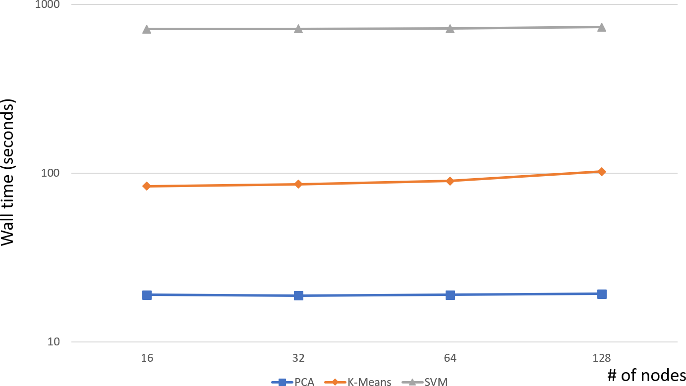
Figure 1: Weak scaling performance (flatter is better) on Titan with the reference implementation.

We found that on Titan, using 8 GB per node was optimal. This left adequate room for the additional needs of each benchmark. To meet the 1024 GB requirement, this meant that we needed to run on a minimum of 128 nodes. However, to get a sense for the weak scaling of the code, we run it at 16, 32, 64, and 128 nodes. Figure 1 shows the results of running the benchmarks on Titan at these node counts, with total problem sizes for the 4 runs of 128, 256, 512, and 1024 GB, respectively. Notice that PCA and SVM are almost entirely flat, while k-means has a slight but noticeable uptick to it. From this, we expect that we could scale each of these out to many more nodes without seeing strong deviations from the flat trend.

Benchmarks	k-means	PCA	SVM
$t_{a}$ (s)	83.8	24.8	631.2
FOM (TB/s)	1.8	6.0	0.24

z

TABLE I: Projected Baseline FOM on Titan

The baseline FOM on Titan is projected as follows. Since the problem size is defined to be larger than 1024 GB and the scaling efficiency for k-means decreases as the node count increases, we choose the minimum number of nodes (128 in our case) for the individual job that can accommodate the input data. As a measurement of throughput, we simultaneously run 30 such jobs, which accounts for about 20$\%$ of Titan’s total node capacity. Afterwards, the average maximum wallclock time $t_{a}$ are calculated for each of the 3 benchmarks. The projected baseline FOM in TB/s for each benchmark on Titan is calculated as $1.024/t_{a}*(18688/128)$. The details for the individual benchmarks are provided in Table I.

III-B Performance Projections on Summit

At the time of writing, Titan is ranked number 7 on the Top500 supercomputer list [39]. And so in some sense, Titan represents the current generation of supercomputers. Even so, it is quite old by computing standards at nearly 6 years of age at the time of writing. To that end, we also ran the benchmarks on two additional, newer OLCF systems: Summit and SummitDev.

Summit, which is not yet available for general use, will be the United States’ new largest supercomputer. While it will officially come online in January of 2019, it is at the time of writing the number 1 machine on the Top500. When fully operational, it will have roughly 4600 IBM nodes. Each node will have two 22-core POWER 9 CPUs 512 GB of system RAM, giving it more than 200,000 cores and more than 2 PB of system RAM. Additionally, each node will have 6 NVIDIA Volta GPUs connected with NVIDIA’s high-speed NVLink, for a total of around 27,000 GPUs. The nodes are connected with a Mellanox EDR InfiniBand interconnect in a non-blocking fat tree topology. Each node is anticipated to have a theoretical peak performance in excess of 40 teraflops. On the other hand, SummitDev is a transitional machine to allow researchers to begin testing and porting codes to a Summit-like architecture. It has 36 nodes, each with two IBM POWER8 CPUs and four NVIDIA Pascal GPUs.

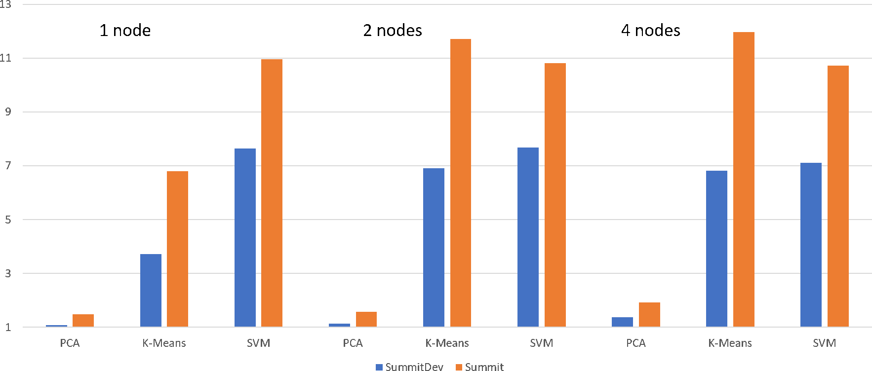
Figure 2: Speedup over the Titan baseline with SummitDev and Summit.

For each of the benchmarks, we use 80 MPI ranks per node and 2 threads per rank on SummitDev, and 42 MPI ranks per node with 4 threads per rank on Summit for the reference implementation, as this was optimal among all configurations we tried.

Figure 2 shows the speedup over the Titan baseline on both SummitDev and Summit. This performance boost comes without any tuning; it is merely the acceleration due to newer, more advanced hardware. The comparisons are node-for-node, in that for example, the 2 nodes plot shows the performance boost of using 2 nodes of SummitDev or Summit versus using 2 nodes of Titan. Each run still uses a problem size of 8 GB per node. We do not scale out to 128 nodes because in the case of SummitDev, we do not have that many.

Several things are immediately striking about these plots. First, k-means and SVM get large performance boosts essentially for free, while PCA receives very little performance boost. This is relatively unsurprising, given our motivations for each benchmark, which we outlined in Section II-A. Also striking is the jump in performance from 1 to 2 nodes for k-means, which is sustained from 2 to 4 nodes. This holds true both for comparisons between the newer systems and the baseline, but also between SummitDev and Summit. This reinforces the suspicion first suggested by Figure 1 that the k-means benchmark has significantly more network communication than the other benchmarks.

Next, we compared the performance of the reference implementation with the popular machine learning package H2O [40]. Like the reference implementations, H2O can be run in a multi-threaded/multi-node combination. However, H2O is written in Java and a REST API for communication, while the reference code’s computationally expensive pieces are written in C and it uses MPI for communication. Throughout on both SummitDev and Summit, we use 80 threads for 1 node and 160 threads per node for the 2 and 4 node case with H2O, as this was optimal among all configurations we tried. Additionally, for k-means we disabled standardization of input as this was adding significantly to its compute time while no such comparable thing was done in the reference code.

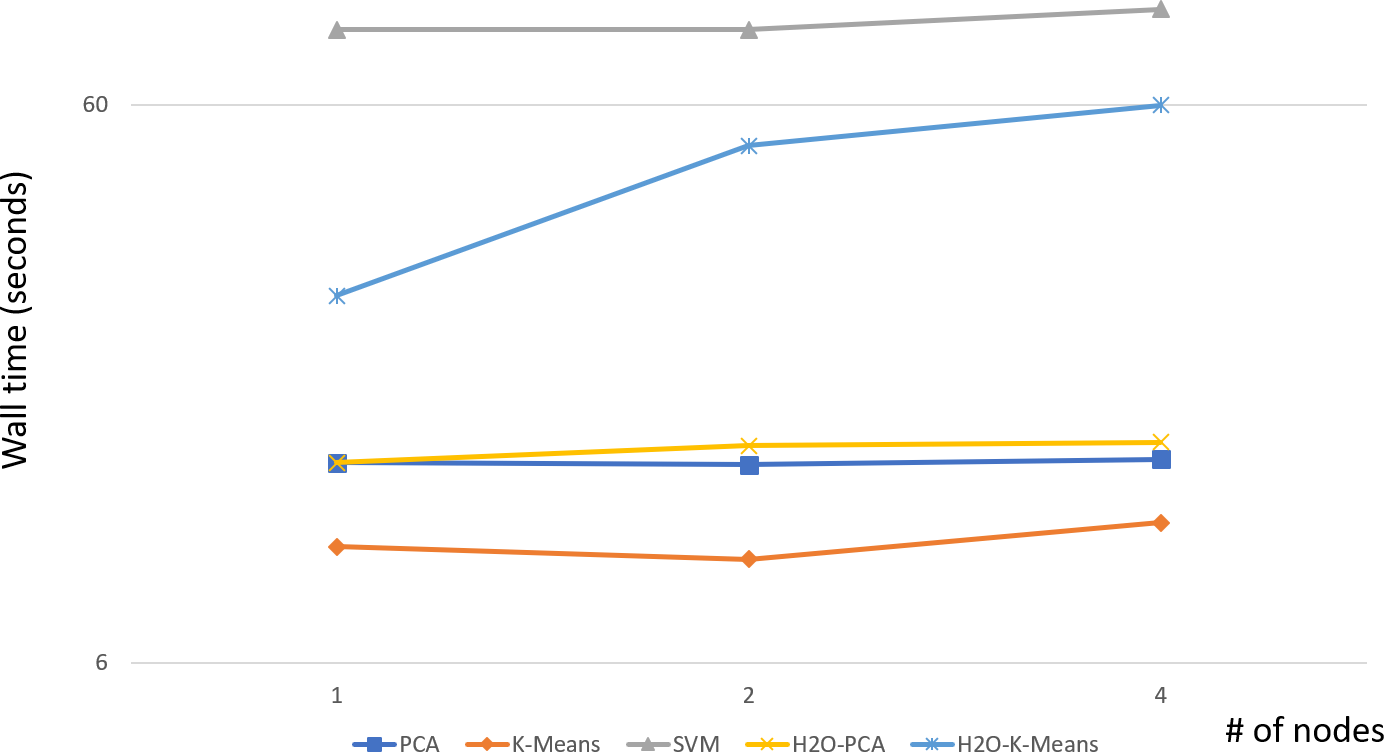
Figure 3: Weak scaling performance (flatter is better) on Summitdev, comparing the reference implementation with H2O.

To compare the two implementations, we run H2O’s PCA and k-means kernels (it does not have a comparable SVM) with the same 8 GB local problem size on SummitDev and examine its weak scaling behavior. Figure 3 shows the results of this test.

First notice that the two PCA kernels are very close in performance. In fact, the two are nearly identical at one node. For 2 and 4 nodes, there is a slight divergence, likely due to the advantage of the reference code in using MPI, which can better utilize the special interconnect hardware. However, the k-means results paint a different picture. The H2O run times are significantly higher than those of the reference implementation. We were unable to determine why, as the number of iterations for each was fixed and we believe the two to be using the same algorithm. It is possible that the H2O implementation is spending a lot of effort in attempting to find better initial cluster assignments. This would likely reduce the number of iterations needed to convergence, even though it makes the initialization more expensive. By comparison, the reference code merely uses a single random initialization. Because our number of iterations in the benchmark is kept artificially low, it is hard to say what exactly is happening here. In the interest of fairness, we believe it is reasonable to give the benefit of the doubt here and assume that the extra work is part of a valid strategy. So although the absolute numbers may not be directly comparable, the relative scaling numbers are. We see the usual slight overall trend upwards in the runtimes for the reference implementation. However, there is a very large jump from 1 to 2 nodes in the H2O implementation. Again, this is likely due to their communication framework not taking advantage of the hardware as MPI can.

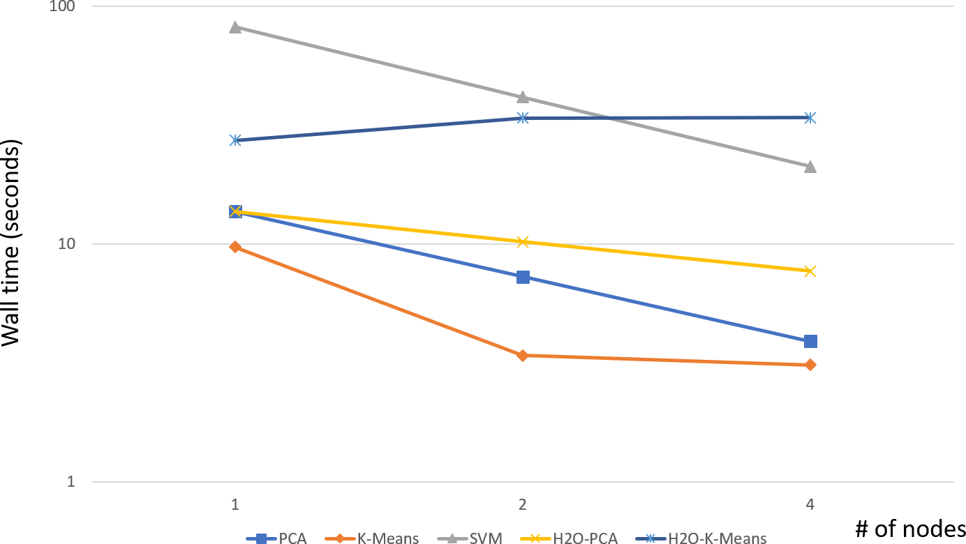
Figure 4: Strong scaling performance (lower is better) on Summitdev, comparing the reference implementation with H2O.

Finally, we made one strong scaling run, the results of which are shown in Figure 4. In this case, we fix the problem size across all node sizes to 8 GB and we use the same rank and threading layout as before. For the reference implementation, we see relatively modest strong scaling from each of the kernels at both 2 and 4 nodes. Again with H2O we see what is likely larger communication overheads reducing the scalability. In all likelihood, both code bases are underperforming in this test due to the small local problem sizes at 4 nodes.

It is possible that more tuning would improve the absolute performance of H2O. However, the poor scaling to multiple nodes that we see particularly in k-means is unlikely to improve because of their current inability to take advantage of the machine’s advanced network fabrics as MPI does. Essentially, H2O was designed for the cloud, not HPC.

IV Modeling Hardware Performance for Big Data Analytics

Finally, we make several more sets of runs using the benchmark kernels in an attempt to understand and model performance of HPC systems for big data analytics. To do this, we again employ Summit and SummitDev, but we include two additional OLCF systems: Percival and Eos. Percival is a 168 node Cray XC40. Each node has a 64 core Intel “Knights Landing” (KNL) Xeon Phi processor with 128 GB of RAM. Eos is a 736 node Cray XC30. Each node has an Intel Xeon processor with 64 GB of RAM. Each system has a Cray Aries interconnect with a Dragonfly topology.

Throughout, we will consider two problem sizes: 8 GB and 64 GB. While these sizes are both relatively small, they are still generally larger than laptop sized problems (particularly when one considers the additional memory required for workspaces and copies). The smaller of the two runs on a single node of each system, and the larger of the two fully saturates at least one node of each. For the power systems, we exclusively use one node for each problem size, while for the Intel systems we use 2 nodes for Percival and 4 nodes for Eos at the 64 GB problem size.

We measure several different potential sources of variation. For one, each system has a different architecture: Power 8 (P8) on SummitDev, Power 9 (P9) on Summit, KNL on Percival, and Xeon on Eos. We also include the problem size as a potential source of variation. Next, we consider different BLAS libraries. On each system, we use OpenBLAS [41] as a baseline, and compare it against a vendor equivalent, namely MKL [42] on the two Intel machines, and ESSL [43] on the two IBM machines. Additionally, we use two different R versions throughout: 3.4.3 and 3.5.1. There was a major internal change in R version 3.5.0 which could affect the performance of several of the kernels, k-means in particular. We also try various threading vs MPI rank schemas. For the Power machines, we use the same strategy as in Section III-B, and for the Intel machines, rather than oversubscribing we use either 1 MPI rank per core and no multi-threaded BLAS, or 1 MPI rank every two cores and 2 BLAS threads. Finally, we treat the different benchmark kernels themselves as a source of variation, using them as proxies for different workloads (e.g. compute vs memory bound).

We pause here to note that we made numerous attempts to utilize the GPUs on the Power machines. Our experiments involved using NVBLAS [44] in various ways. However, we were unable to ever achieve better performance than CPU-only configurations using OpenBLAS. We even made several modifications to the benchmark kernel codes to try to encourage better performance with the GPUs. For example, much of the computation in the SVM code boils down to a fairly large matrix-vector product. In the code, this was calling R’s matrix product function %*%, which internally was resolving to the BLAS primitive DGEMV. Since DGEMV is not supported by NVBLAS, we modified the benchmark kernel to directly call DGEMM so that it would evaluate on the GPU. However, the performance results were mixed, and we believe that at a minimum, more experimentation is necessary before conclusions can be drawn. We know that creating specialized kernels specifically for the GPU will yield good performance, but for the purpose of this demonstration, we wished only to make relatively minor modifications to the code to get it to run. Section A describes our use of NVBLAS in slightly more detail.

Returning to the task at hand, we note explicitly all possible combinations of parameters tried. For Percival and Eos, we measure Architecture (KNL and Xeon), Problem size (8 GB and 32 GB), BLAS library (OpenBLAS and MKL), R version (3.4.3 and 3.5.1), Number of threads (1 or 2), and Workload (PCA, KMEANS, and SVM). For Summit and SummitDev, we measure Architecture (P8 and P9), Problem size (8 GB and 64 GB), BLAS library (OpenBLAS and ESSL), R version (3.4.3 and 3.5.1), Number of Threads (1, 2, 4, and 8), and Workload (PCA, KMEANS, and SVM). For each combination of inputs across both systems, we measure the maximum run time and divide it by the problem size for a performance measure in GB/s.

After performing all of the necessary runs, we fit two linear models, one for the Power systems and one for the Intel systems. We select an optimal model by AIC [45] in a stepwise manner considering only the first order terms. The final models are $\log\left(Perf_{Intel}\right)$ is a linear combination of $Size$ and $Workload$, while $\log\left(Perf_{Power}\right)$ is a linear combination of $Architecture$, $Size$, and $Workload$.

Focusing fist on the Intel model, we note that the final model has an Adjusted R-squared of 0.881 with an overall F-statistic of 82.02 (p-value $1.476e-14$). The ANOVA table for the model is given in Table II. Unsurprisingly, the problem size and workload significant sources of variation. The choice of BLAS library and R version being non-significant sources of variation are perhaps a little surprising. However, the architecture being non-significant is deeply shocking. Evaluating the data, it is not clear exactly how this is so, and more study is warranted to understand this behavior.

	Sum Sq	Df	F value	Pr($>$F)
Problem Size	6.92	1	36.91	0.0000
Workload	40.43	2	107.78	0.0000
Residuals	5.63	30

TABLE II: ANOVA table for the Intel systems.

For the Power model, we note that the final model has an Adjusted R-squared of 0.954 with an overall F-statistic of 698.1 (p-value $<2.2e-16$). The ANOVA table for the model is given in Table III. As with the Intel model, the problem size and workload are, unsurprisingly, statistically significant sources of variation. And again, the R version and BLAS library were not found to be significant sources of variation. However, as one might expect, the system architecture (P8 vs P9) and the number of threads were found to be significant.

	Sum Sq	Df	F value	Pr($>$F)
Architecture	27.68	1	519.23	0.0000
Workload	150.08	2	1407.47	0.0000
Problem Size	0.67	1	12.56	0.0005
Threads	1.06	1	19.82	0.0000
Residuals	8.64	162

TABLE III: ANOVA table for the Power systems.

What we can reasonably conclude from these two models is that the node-level performance of an HPC system for big data analytics codes like ours is highly problem size and workload dependent. CPU architecture may play some role, but perhaps not as much as one might expect. Other concerns commonly found at HPC centers like choice of boutique BLAS library may add little value, so long as one is not using the reference implementation of the BLAS. Trading off MPI ranks for BLAS threads or oversubscribing the cores with BLAS threads may lead to performance improvements, but this appears to be architecture dependent.

Finally, we average all of the runs per system across groups so that we get a single performance number (average GB/s) for each of the three benchmark kernels for each of the two systems. Figure 5 shows the comparison of these values. In each case, the Power systems are quite competitive in terms of average performance.

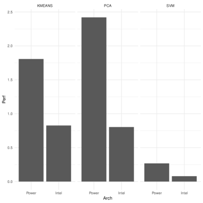
Figure 5: Comparison of average performance across Intel systems (Percival/Eos) and Power systems (Summit/SummitDev) on the benchmarks (higher is better).

It is worth noting that one key issue this analysis leaves out is cost, of both the hardware and power consumption (e.g., flops per watt). We were unable to obtain this information, and it is likely to make this story much more complex. However, if price is no concern (and in HPC, that is sadly sometimes the case), then the Power systems do appear to be quite fast for big data analytics.

V Conclusions

We have described a new set of high performance big data analytics benchmarks designed for the peculiarities of HPC systems. We have attempted to motivate the necessity for this new work, in light of the large prior work already publicly available. In running these benchmarks on existing HPC resources, we have seen very good weak scaling and some modest strong scaling at the low node counts we used during evaluation. We also used the benchmark kernels to attempt to understand and model performance of HPC systems for big data analytics as we define it. Invoking Szilard Pafka, we concede that the benchmarks are not perfect, but we hope that they are useful.

Finally, we note that the assessment of these benchmarks on Summit is preliminary, and therefore the related data and observations reported in this paper are subject to change after more thorough studies are performed.

Appendix A Artifact Description

Throughout, we used various versions of the GNU compiler collection, each of which is at least version 4.8.

In all cases, we used R version 3.4.3, except in section IV where we compare performance between 3.4.3 and 3.5.1. We used pbdMPI version 0.3-8, although we tested several versions and determined that these different versions did not contribute to the performance variation. This was not surprising given the changes across recent pbdMPI versions, so we did not bother to include it in the final performance analysis above. We used kazaam version 0.2-0, which included several modifications specifically for these benchmarking efforts, as noted in Section IV. The following configure line was used for each build of R:

⬇

./configure –with-x=no \

–enable-R-shlib=no \

–enable-memory-profiling=no

For systems libraries, we used OpenBLAS version 0.2.20 across all systems. On Percival (Intel KNL), where use of MKL was noted, we used MKL 2018 initial release and on Eos (Intel Xeon) we used MKL 2018 update 1. On SummitDev (P8) and Summit (P9) where use of ESSL was noted, we used ESSL 5.5.0. For MPI libraries, we used Intel MPI on Percival and Eos, with versions corresponding to the MKL release versions noted above. On Summit and Summitdev we used OpenMPI 3.1.0.

For the NVBLAS tests on Summit and SummitDev mentioned in Section IV, we used the following nvblas.conf file:

⬇

NVBLAS_LOGFILE nvblas.log

NVBLAS_CPU_BLAS_LIB /path/to/libopenblas.so

NVBLAS_GPU_LIST ALL

NVBLAS_TRACE_LOG_ENABLED

#NVBLAS_AUTOPIN_MEM_ENABLED

#NVBLAS_TILE_DIM 2048

and the R_gpu script:

⬇

#!/bin/sh

LD_PRELOAD=/path/to/libnvblas.so

NVBLAS_CONFIG_FILE=/path/to/nvblas.conf R ”$@”

References

- [1] “Fact sheet: Collaboration of oak ridge, argonne, and livermore (coral),” https://www.energy.gov/downloads/fact-sheet-collaboration-oak-ridge-argonne-and-livermore-coral, accessed: 2018-03-05.
- [2] S. R. Sukumar, M. A. Matheson, R. Kannan, and S. H. Lim, “Mini-apps for high performance data analysis,” in 2016 IEEE International Conference on Big Data (Big Data), Dec 2016, pp. 1483–1492.
- [3] G. Fox, J. Qiu, S. Jha, S. Ekanayake, and S. Kamburugamuve, “Big data, simulations and hpc convergence,” in Big Data Benchmarking. Springer, 2015, pp. 3–17.
- [4] S. Huang, J. Huang, J. Dai, T. Xie, and B. Huang, “The hibench benchmark suite: Characterization of the mapreduce-based data analysis,” in Data Engineering Workshops (ICDEW), 2010 IEEE 26th International Conference on. IEEE, 2010, pp. 41–51.
- [5] A. Ghazal, T. Rabl, M. Hu, F. Raab, M. Poess, A. Crolotte, and H.-A. Jacobsen, “Bigbench: towards an industry standard benchmark for big data analytics,” in Proceedings of the 2013 ACM SIGMOD international conference on Management of data. ACM, 2013, pp. 1197–1208.
- [6] L. Wang, J. Zhan, C. Luo, Y. Zhu, Q. Yang, Y. He, W. Gao, Z. Jia, Y. Shi, S. Zhang et al., “Bigdatabench: A big data benchmark suite from internet services,” in High Performance Computer Architecture (HPCA), 2014 IEEE 20th International Symposium on. IEEE, 2014, pp. 488–499.
- [7] M. Folk, A. Cheng, and K. Yates, “Hdf5: A file format and i/o library for high performance computing applications,” in Proceedings of supercomputing, vol. 99, 1999, pp. 5–33.
- [8] R. Rew, E. Hartnett, J. Caron et al., “Netcdf-4: Software implementing an enhanced data model for the geosciences,” in 22nd International Conference on Interactive Information Processing Systems for Meteorology, Oceanograph, and Hydrology, 2006.
- [9] T. G. Armstrong, V. Ponnekanti, D. Borthakur, and M. Callaghan, “Linkbench: a database benchmark based on the facebook social graph,” in Proceedings of the 2013 ACM SIGMOD International Conference on Management of Data. ACM, 2013, pp. 1185–1196.
- [10] M. Capotă, T. Hegeman, A. Iosup, A. Prat-Pérez, O. Erling, and P. Boncz, “Graphalytics: A big data benchmark for graph-processing platforms,” in Proceedings of the GRADES’15. ACM, 2015, p. 7.
- [11] S. Pafka, “Simple/limited/incomplete benchmark for scalability, speed and accuracy of machine learning libraries for classification,” https://github.com/szilard/benchm-ml, accessed: 2018-03-07.
- [12] ——, “Machine learning software in practice: Quo vadis?” in Proceedings of the 23rd ACM SIGKDD International Conference on Knowledge Discovery and Data Mining. ACM, 2017, pp. 25–25.
- [13] M. Zaharia, R. S. Xin, P. Wendell, T. Das, M. Armbrust, A. Dave, X. Meng, J. Rosen, S. Venkataraman, M. J. Franklin et al., “Apache spark: a unified engine for big data processing,” Communications of the ACM, vol. 59, no. 11, pp. 56–65, 2016.
- [14] P. Xenopoulos, J. Daniel, M. Matheson, and S. Sukumar, “Big data analytics on hpc architectures: Performance and cost,” in 2016 IEEE International Conference on Big Data (Big Data), Dec 2016, pp. 2286–2295.
- [15] J. L. Reyes-Ortiz, L. Oneto, and D. Anguita, “Big data analytics in the cloud: Spark on hadoop vs mpi/openmp on beowulf,” Procedia Computer Science, vol. 53, pp. 121–130, 2015.
- [16] A. Gittens, A. Devarakonda, E. Racah, M. Ringenburg, L. Gerhardt, J. Kottalam, J. Liu, K. Maschhoff, S. Canon, J. Chhugani et al., “Matrix factorizations at scale: A comparison of scientific data analytics in spark and c+ mpi using three case studies,” in Big Data (Big Data), 2016 IEEE International Conference on. IEEE, 2016, pp. 204–213.
- [17] F. Pedregosa, G. Varoquaux, A. Gramfort, V. Michel, B. Thirion, O. Grisel, M. Blondel, P. Prettenhofer, R. Weiss, V. Dubourg et al., “Scikit-learn: Machine learning in python,” Journal of machine learning research, vol. 12, no. Oct, pp. 2825–2830, 2011.
- [18] M. K. C. from Jed Wing, S. Weston, A. Williams, C. Keefer, A. Engelhardt, T. Cooper, Z. Mayer, B. Kenkel, the R Core Team, M. Benesty, R. Lescarbeau, A. Ziem, L. Scrucca, Y. Tang, C. Candan, and T. Hunt., caret: Classification and Regression Training, 2017, r package version 6.0-78. [Online]. Available: https://CRAN.R-project.org/package=caret
- [19] M. Abadi, P. Barham, J. Chen, Z. Chen, A. Davis, J. Dean, M. Devin, S. Ghemawat, G. Irving, M. Isard et al., “Tensorflow: A system for large-scale machine learning.” in OSDI, vol. 16, 2016, pp. 265–283.
- [20] N. Valigi, “Coral-2 benchmarks,” https://nicolovaligi.com/gradient-boosting-tensorflow-xgboost.html, accessed: 2018-03-07.
- [21] G. M. Kurtzer, V. Sochat, and M. W. Bauer, “Singularity: Scientific containers for mobility of compute,” PloS one, vol. 12, no. 5, p. e0177459, 2017.
- [22] R. S. Canon and D. Jacobsen, “Shifter: containers for hpc,” Proceedings of the Cray User Group, 2016.
- [23] T. Chen and C. Guestrin, “Xgboost: A scalable tree boosting system,” in Proceedings of the 22nd acm sigkdd international conference on knowledge discovery and data mining. ACM, 2016, pp. 785–794.
- [24] R. Fisher and M. Marshall, “Iris data set,” RA Fisher, UC Irvine Machine Learning Repository, vol. 440, 1936.
- [25] N. Halko, P.-G. Martinsson, and J. A. Tropp, “Finding structure with randomness: Probabilistic algorithms for constructing approximate matrix decompositions,” SIAM review, vol. 53, no. 2, pp. 217–288, 2011.
- [26] W. M. Rand, “Objective criteria for the evaluation of clustering methods,” Journal of the American Statistical association, vol. 66, no. 336, pp. 846–850, 1971.
- [27] R Core Team, R: A Language and Environment for Statistical Computing, R Foundation for Statistical Computing, Vienna, Austria, 2012.
- [28] R. Muenchen, “The popularity of data analysis software,” http://r4stats.com/articles/popularity, 2017, accessed: 2017-08-28.
- [29] S. Cass, “The 2017 top programming languages,” https://spectrum.ieee.org/computing/software/the-2017-top-programming-languages, 2017.
- [30] ——, “The 2018 top programming languages,” https://spectrum.ieee.org/at-work/innovation/the-2018-top-programming-languages, 2018.
- [31] W. Gropp, E. Lusk, and A. Skjellum, Using MPI: Portable Parallel Programming with the Message-Passing Interface. Cambridge, MA, USA: MIT Press Scientific And Engineering Computation Series, 1994.
- [32] W.-C. Chen, G. Ostrouchov, D. Schmidt, P. Patel, and H. Yu, “pbdMPI: Programming with big data – interface to MPI,” 2012, R Package, URL http://cran.r-project.org/package=pbdMPI.
- [33] G. Ostrouchov, W.-C. Chen, D. Schmidt, and P. Patel, “Programming with big data in R,” 2012, uRL http://r-pbd.org/.
- [34] D. Schmidt, W.-C. Chen, M. Matheson, and G. Ostrouchov, “kazaam: Tools for tall distributed matrices,” 2017, R package version 0.2-0. [Online]. Available: https://cran.r-project.org/package=kazaam
- [35] C. L. Lawson, R. J. Hanson, D. R. Kincaid, and F. T. Krogh, “Basic linear algebra subprograms for Fortran usage,” ACM Transactions on Mathematical Software (TOMS), vol. 5, no. 3, pp. 308–323, 1979.
- [36] E. Anderson, Z. Bai, C. Bischof, L. S. Blackford, J. Demmel, J. Dongarra, J. D. Croz, A. Greenbaum, S. Hammarling, A. McKenney, and D. Sorensen, LAPACK Users’ Guide, 3rd ed. Society for Industrial and Applied Mathematics, 1999.
- [37] X. Meng, J. Bradley, B. Yavuz, E. Sparks, S. Venkataraman, D. Liu, J. Freeman, D. Tsai, M. Amde, S. Owen et al., “Mllib: Machine learning in apache spark,” The Journal of Machine Learning Research, vol. 17, no. 1, pp. 1235–1241, 2016.
- [38] “Coral-2 benchmarks,” https://asc.llnl.gov/coral-2-benchmarks/, accessed: 2018-03-05.
- [39] J. J. Dongarra, H. W. Meuer, E. Strohmaier et al., “Top500 supercomputer sites,” Supercomputer, vol. 13, pp. 89–111, 1997.
- [40] S. Aiello, C. Click, H. Roark, and L. Rehak, “Machine learning with python and h20,” H2O. ai Inc, 2016.
- [41] Z. Xianyi, W. Qian, and Z. Chothia, “Openblas,” URL: http://xianyi. github. io/OpenBLAS, 2014.
- [42] Intel Corporation, “Intel math kernel library (intel mkl),” 2018, uRL http://software.intel.com/en-us/intel-mkl/.
- [43] IBM, “Engineering and scientific subroutine library,” 2018, uRL https://www.ibm.com/support/knowledgecenter/en/SSFHY8/essl_welcome.html.
- [44] NVIDIA, “Nvblas library,” URL: http://docs.nvidia.com/cuda/nvblas/, 2018.
- [45] H. Akaike, “A new look at the statistical model identification,” IEEE transactions on automatic control, vol. 19, no. 6, pp. 716–723, 1974.