Time-dependent atomic diffusion in the atmospheres of CP stars. A big step forward: introducing numerical models including a stellar mass loss

Abstract

Calculating abundance stratifications in ApBp/HgMn star atmospheres, we are considering mass-loss in addition to atomic diffusion in our numerical code in order to achieve more realistic models. These numerical simulations with mass-loss solve the time dependent continuity equation for plane-parallel atmospheres; the procedure is iterated until stationary concentrations of the diffusing elements are obtained throughout a large part of the stellar atmosphere. We find that Mg stratifications in HgMn star atmospheres are particularly sensitive to the presence of a mass-loss. For main-sequence stars with $T_{\rm{eff}}\approx 12000$ K, the observed systematic mild underabundances of this element can be explained only if a mass-loss rate of around $4.2\,10^{-14}$ solar mass per year is assumed in our models. Numerical simulations also reveal that the abundance stratification of P observed in the HgMn star HD 53929 may be understood if a weak horizontal magnetic field of about 75 G is present in this star. However, for a better comparison of our results with observations, it will be necessary to carry out 3D modelling, especially when magnetic fields and stellar winds – which render the atmosphere anisotropic – are considered together.

1 Introduction

The modelling of chemically peculiar (CP) star atmospheres including atomic diffusion constitutes a long-standing challenge. Between the first paper by Michaud (1970) and the most recent calculations of Alecian & Stift (2017), great progress has been made. However, as pointed out in the conclusions of Michaud et al. (2015) and in several theoretical works on this subject, detailed observed abundances of individual CP stars are still difficult to reproduce in numerical models, even in the case HgMn stars which are considered as the simplest ones to model. Theses difficulties are partly due the fact that atomic diffusion is a very slow process, therefore very sensitive to any perturbation due to other physical processes such as macroscopic motions (even weak turbulence, convection, wind or mass-loss), magnetic fields, etc. when models of inhomogeneous elements distributions are computed in view of reproducing atmospheres of real CP stars. Theoreticians agree that atomic diffusion must not be considered as acting alone. Although there have been significant advances in the understanding of the main trends in abundance peculiarities observed in CP stars – as for instance the dependence of Mn overabundances on $T_{\rm{eff}}$ in HgMn stars (Alecian & Michaud, 1981; Smith & Dworetsky, 1993), or the stratified abundances of Mg, Si, Ca, Ti, Cr, Fe, and Ni at $8000$ K and $12000$ K (LeBlanc et al., 2009) – numerical modelling of atomic diffusion in atmospheres continues to improve only slowly. Step by step the calculations becomes more sophisticated with the final goal to provide theoretical metal abundance patterns which can be confronted with observations of individual stars.

Our most recent progress in numerical modelling of CP star atmospheres has been the first model of theoretical 3D distributions of Cr and Fe in atmospheres with a non-axisymmetric magnetic field (Alecian & Stift, 2017). In this paper, it was shown that, even if equilibrium solutions favour higher concentrations of metals in regions where the magnetic field is horizontal (which, according to some authors, is not observed, see Kochukhov & Ryabchikova 2018), this is expected to happen in most cases so high up in the atmosphere that it could hardly be detected. It appears that the photosphere might rather be dominated by abundance patches due to atomic diffusion in magnetic fields of non-axisymmetric geometry. At this point one should however keep in mind that virtually all previous attempts to quantitatively predict abundance stratifications due to atomic diffusion Alecian & Stift (2017) have used equilibrium solutions (see for instance LeBlanc et al. 2009), a method that might legitimately be questioned. In the past, we have often warned in our papers against mis- or over-interpretations that can be drawn from equilibrium solutions. Indeed, equilibrium solutions must be interpreted as mapping only the maximum abundances that can possibly be supported by the radiation field. In some cases, this may correspond to the real element distribution, but not so in the majority of cases. Still, in a number of publications observations have been confronted with equilibrium results and it has hastily been concluded that theoretical predictions are not confirmed by observations.

We are convinced that stationary solutions obtained with extremely time-consuming calculations of time-dependent atomic diffusion (which can differ widely from equilibrium results) will generally be much closer to what happens in real atmospheres; this approach is discussed in Alecian et al. 2011 and Stift & Alecian 2016. Let us recall what Alecian & Stift (2017) have emphasised in their conclusions, viz. that the next step in numerical modelling must consist in the inclusion of stellar mass-loss which is well known to compete with atomic diffusion in many types of CP stars (see Vauclair, 1975; Michaud et al., 1983; Babel, 1992; Alecian, 1996; Landstreet et al., 1998; Vick et al., 2010; Alecian, 2015). The mass-loss rates, which have not yet been directly observed for main-sequence CP stars with $T_{\rm{eff}}\mathrel{\hbox{\raise 2.58334pt\hbox{$<$}\kern-7.74998pt\lower 2.15277pt\hbox{$\sim$}}}18000$ K, have been estimated – by means of numerical modelling of stellar internal structure – by Vick et al. (2010) to lie around $5.0\,10^{-14}$ solar mass per year for hot AmFm stars ($T_{\rm{eff}}<10000$ K). X-ray emission possibly related to the existence of a wind has been detected in an ApBp star (IQ Aur) as discussed by Babel & Montmerle (1997). The mass-loss rate probably increases with effective temperature. For instance, for He-rich stars, which are the hottest main-sequence CP stars ($T_{\rm{eff}}\mathrel{\hbox{\raise 2.58334pt\hbox{$>$}\kern-7.3194pt\lower 2.15277pt\hbox{$\sim$}}}18000$ K), it has been estimated at about $10^{-12}$ solar mass per year (see Vauclair, 1975). Winds are detected through the study of X-ray emission in early B and hotter stars (see for example Oskinova et al., 2011).

The present work addresses for the first time the build-up of abundance stratifications in stellar atmospheres due to time-dependent atomic diffusion in conjunction with mass-loss. Our study concerns only ApBp stars (including HgMn stars). In some other CP stars (viz. the AmFm), the mixing of external layers prevents atomic diffusion of metals to be efficient in the atmospheres. For stars with $T_{\rm{eff}}\mathrel{\hbox{\raise 2.58334pt\hbox{$>$}\kern-7.3194pt\lower 2.15277pt\hbox{$\sim$}}}18000$ K, abundances cannot stratify significantly in the atmospheres due to the high wind velocity. Actually, Babel (1992) has been the first to consider a stellar wind in presence of atomic diffusion in magnetic atmospheres in order to explain the observed Ca, Cr, Fe and Sr lines in 53 Cam (a cool Ap star with $T_{\rm{eff}}\approx 8500$ K). This pioneering work considered equilibrium solutions, assuming a weak inhomogeneous wind as a free parameter, and proposed a wind model corresponding to a mass-loss rate of about $3\,10^{-15}$ solar mass per year at the poles to fit the line spectra. In the present work, we base our findings on time-dependent numerical simulations for plane-parallel atmospheres, assuming various mass-loss rates with essentially no magnetic fields (which may be relevant for HgMn stars) but we also present a couple of calculations with very weak and with moderate magnetic fields. The magnetic case accompanied by an anisotropic wind will be considered in a forthcoming paper.

In Sec. 2 we detail how mass-loss is introduced into the equations, and in Sec. 2.1 we present the modifications to our code CaratMotion. The numerical results for a typical Bp star are presented in Sec. 3. In Sec. 4, we discuss the case of the HgMn star HD 53929 for which Ndiaye et al. (2018) have derived empirical vertical stratifications of P and Fe. We finally propose a general discussion in Sec. 5, followed by concluding remarks in Sec. 6.

2 Modelling the mass-loss

At present it does not appear feasible to develop a fully self-consistent treatment of atomic diffusion in combination with mass-loss. However, to a first approximation, the velocity of the stellar wind (in cgs units) is given by

$$V_{\rm wind}=\frac{\dot{M}\,M_{\sun}}{4\pi\rho R^{2}}=\frac{\dot{M}\,g}{4\pi\rho\,G(M/M_{\sun})}\,,$$ (1)

where $\dot{M}$ stands for the mass-loss rate (solar mass per second). $G$ is the gravitational constant, $\rho$ denotes the mass density at a given layer in the atmosphere, $M$ the stellar mass, $R$ the stellar radius, $g$ the stellar gravitational acceleration. Keeping in mind that the depth of a stellar atmosphere is negligible in relation to the stellar radius, our formula expresses the fact that the mass flux $V_{w}\rho=(dM/dt)/A$ – with $A$ the stellar surface area – through the atmospheric layers remains constant. This approximation has been used several times in the framework of atomic diffusion modelling (see for instance Vauclair, 1975; Michaud et al., 1983; Alecian, 1986; Vick et al., 2010). At this stage, we do not need to adopt any hypothesis as to the structure of the wind (isotropy, homogeneity or time dependence). The mass-loss rate is just a free parameter fixing the wind velocity according to the depth in our plane-parallel models.

For a given atmospheric model ($T_{\rm eff}$, $\log g$) and corresponding mass $M$, the formula for the wind velocity becomes

$$V_{\rm wind}=C/\rho.$$ (2)

In order to determine $M$ and thence the factor $C$ we resorted to Schaller et al. (1992) who provide a grid of evolutionary tracks for various stellar masses. Effective temperature $T_{\rm eff}$ and gravitational acceleration $\log g$ – which define our atmospheric models – yield the stellar luminosity via

$$\log(L/L_{\sun})=-10.607-\log g+\log(M/M_{\sun})+4\,\log T_{\rm eff}\,.$$ (3)

The $\log(L/L_{\sun})$ values for the given stellar $T_{\rm eff}$ and various masses represented in the evolutionary grid are determined by interpolation, resulting in a relation $\log g$ vs. $M$. The mass corresponding to the atmospheric parameters is calculated by interpolation in this relation. For instance, in Sec. 3, we use a model atmosphere with $T_{\rm eff}=12000$ K and $\log g=4.0\,$. Equ. 3 leads to a stellar mass of 3.4 solar masses, hence the factor $C$ in Eq. 2 becomes $\approx 1.1\,10^{-14}$ for a mass loss rate of $10^{-16}$ solar mass per year.

For the star HD 53929 discussed in Sec. 4, with $T_{\rm eff}=12700$ K and $\log g=3.71$ (Ndiaye et al., 2018) we have $C\approx 4.64\,10^{-15}$, again assuming a mass loss rate of $10^{-16}$ solar mass per year.

2.1 Numerics

Let us recall that our CaratMotion code derives from Carat and CaratStrat which calculate radiative accelerations and diffusion velocities; the physics included in these codes are described in detail in Alecian & Stift (2004) and Stift & Alecian (2012). The numerics of CaratMotion have been presented in Alecian et al. (2011). To ensure self-consistency between chemical stratifications and atmospheric structure, the atmosphere is recalculated after each time step, based on the new abundances, and the atomic line opacities updated accordingly. It comes as no surprise that time-dependent atomic diffusion can prove very expensive, a complete run taking up to 300 and more days mono-processor time on a modern server. Since not all parts of the code can be completely parallelised, it makes no sense to run it on machines doted with hundreds of processors. Instead, executing several jobs concurrently on a dedicated 64 core server minimises idle cpus. Obviously this severely constrains the scope of our simulations which cannot encompass the bulk of ApBp stars, but is limited to a moderate number of well chosen cases.

It proved quite straightforward to adapt the numerical scheme for the modelling of time-dependent atomic diffusion as employed by Stift et al. (2013) in order to accommodate mass-loss. We recall that our models are self-consistent for abundance stratifications and computed at each time-step with Kurucz’s Atlas12 code (Kurucz 2005, Bischof 2005). All chemical elements are transported with the same positive velocity $V_{\rm wind}$; a positive or negative diffusion velocity $V_{\rm elem}$ has to be added for the “diffusing” elements. As an example, in the case of HD 53929 where we are interested in the diffusion of phosphorus and iron only, the donor-cell scheme has to be applied to 3 elements, with H in addition to P and Fe (it will be Mg and Fe in the case discussed in Sec. 3). Since abundances in our numerical code CaratMotion are defined with respect to hydrogen one just has to update the hydrogen number density to obtain at the same time the new number densities of all the other elements, except P and Fe. The latter are calculated by substituting the diffusion velocity in the continuity equation by $V_{\rm wind}+V_{\rm P}$ and $V_{\rm wind}+V_{\rm Fe}$ respectively.

3 Build-up of abundance stratifications assuming mass-loss

The abundance stratifications build-up assuming a mass-loss compared to the case without mass-loss (as recently discussed by Stift & Alecian, 2016), essentially differs by the fact that the stationary solution can hardly converge to equilibrium (zero, or very small particle flux), except for elements that are very weakly supported in the upper atmosphere by the radiation field (such as for helium, see Vauclair, 1975). That is due to the fact that mass-loss imposes a positive flux of particles even if diffusion velocity is close to zero. Therefore, the presence of mass-loss facilitates the escape of overabundant metals from the atmosphere and tends in most cases to produce lower vertical abundance stratification contrasts. In some cases, as for He previously mentioned, mass-loss can compensate gravitational settling (negative diffusion velocity) and make elements overabundant that would sink towards deeper layers in the absence of mass-loss. Detailed stratifications depend on the relative strength and sign of diffusion and wind velocities at each depth point, When the mass-loss rate is too high (generally it increases with effective temperature), atomic diffusion is no longer able to produce abundance stratifications, since matter flux from deeper layers erases abundance changes faster than atomic diffusion can produce them. In this case, the star presents normal abundances. This is believed to be the cause of the higher $T_{\rm eff}$ cutoff of the CP phenomenon.

Our numerical code CaratMotion models the time-dependent abundance stratification process in a realistic, strongly non-linear way, from a starting time when abundances are generally assumed to be vertically homogeneous and solar – with non-constant particle flux throughout the atmosphere – to a final time when particle fluxes become constant and abundances stratified. Thereafter, stratifications no longer evolve over the timescales considered (a small fraction of the main-sequence life, see below); this is what we call a stationary solution. Even though the numerical process is expensive and necessitates large amounts of cpu time, quite often the time-dependent diffusion calculations converge to a stationary solution after a reasonable number of time steps, corresponding to a very short physical time (from some tens of years to some thousands, depending on the element) compared to the characteristic evolutionary time for the internal structure (or stellar age). Hereafter, we present only the final stationary solutions, assuming that they correspond to the observed abundance stratifications, transient phases having a very small chance of being observed.

3.1 Abundances of Mg and Fe in non-magnetic atmospheres

Figure 1: Mg abundance stratification (stationary solutions) vs. the logarithm of the optical depth at 5000 Å as a function of various mass-loss rates (model with $T_{\rm{eff}}=12000$ K, and $\log{g}=4.0$). Panel (a) shows the Mg stratifications for 5 different mass-loss rates (1.7, 1.28, 0.85, 0.425, 0.17 in units of $10^{-13}$ solar mass per year). The vertical thick grey bar corresponds to observations of Mg overabundances in HgMn stars having approximately the same $T_{\rm{eff}}$ and $\log{g}$ . The equilibrium solution (EQ) – heavy dash-dot-dot grey line – is also shown (see text). Panel (b) presents the same stratifications as panel (a) except for the lowest mass-loss rate, but with a different vertical scale.

HgMn stars are considered non-magnetic CP stars and should therefore be easier to model. Some authors (Mathys & Hubrig, 1995) have claimed detection of a magnetic field in one HgMn star, but this has not yet been confirmed. On the other hand, Alecian (2013) proposed that a weak magnetic field could explain the possible existence of high altitude spot-like clouds in HgMn stars. In this section, we assume that HgMn stars are strictly non-magnetic.

Looking at the abundance anomalies in HgMn stars, it appears that the abundance of Mg is very often close to the solar value or slightly underabundant (see the compilation of Ghazaryan & Alecian, 2016). However, since according to Alecian (2015) Mg is only weakly supported by the radiation field in the line forming region, it should be systematically strongly underabundant when diffusion is supposed to act alone. Therefore it is interesting to test the role of mass-loss for this element.

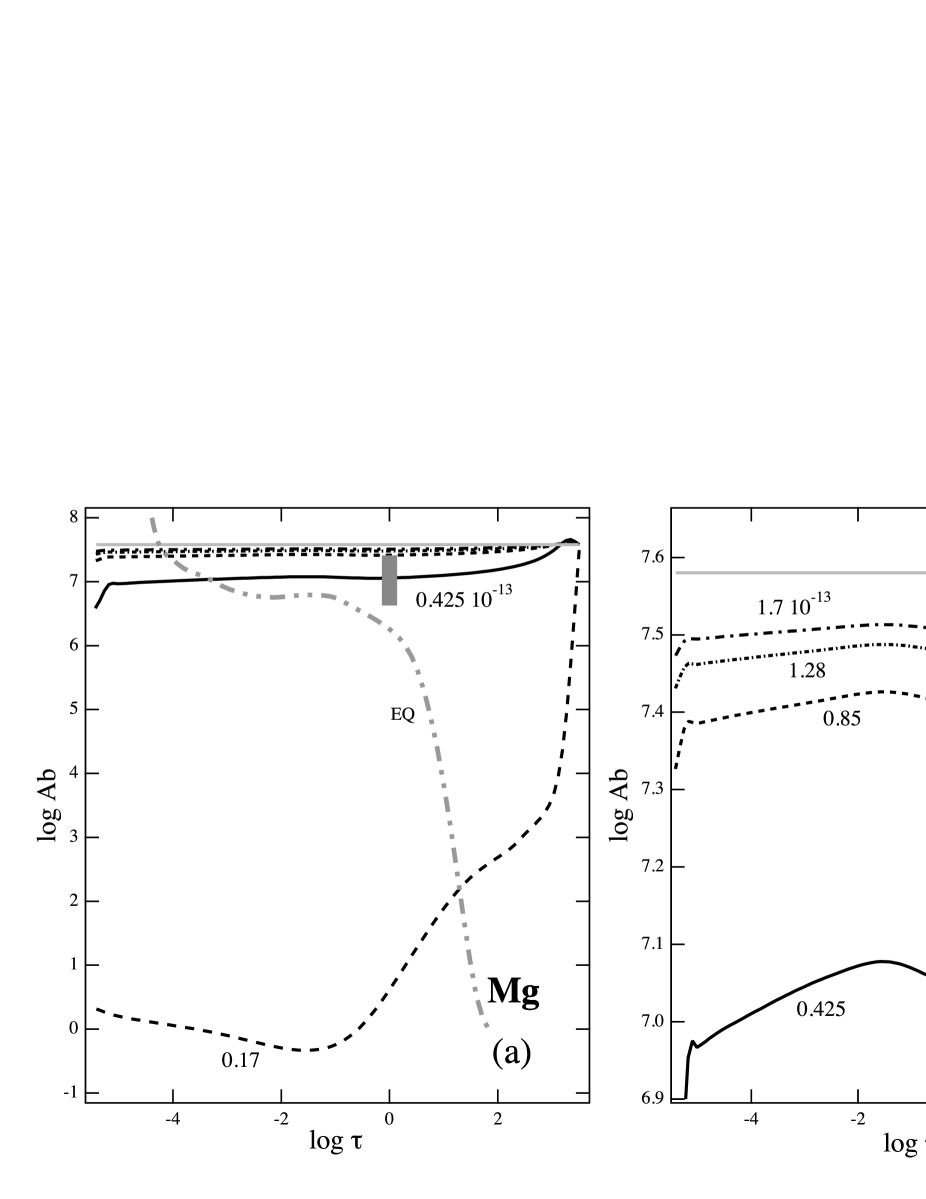
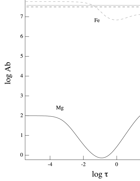
Stationary solutions for various mass-loss rates in an atmosphere with $T_{\rm{eff}}=12000$ K, and $\log{g}=4.0$ are shown in Figs. 1 to 4. Since a global mass flow (here the wind) reduces vertical abundance contrasts, it improves the numerical stability of the calculations. Thanks to the wind, many calculations which become numerically unstable (or do not converge within some reasonable cpu time) in the absence of mass-loss now become possible. In this study, we have succeeded in calculating stationary solutions for Mg and Fe when mass-loss rates are higher than $0.17\,10^{-13}$ solar mass per year. Although this lower limit seems rather far removed from the zero mass-loss case which we would also have liked to model, our results appear to justify the claim that lower mass-loss rates are unlikely to fit the majority of observed abundances of Mg and Fe (see our discussion in Sec. 5.1).

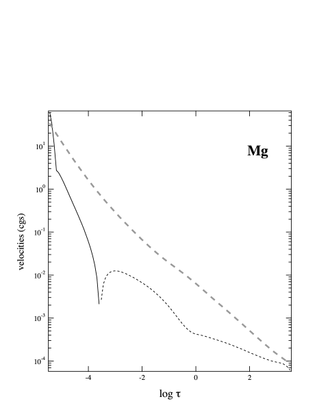
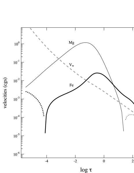
On account of the time-consuming nature of our numerical calculations, we cannot afford to explore the domain of possible mass-loss rates and their effect on the various chemical elements in much detail. In a first step, we have chosen 5 values starting from the lowest rate of $0.17\,10^{-13}$ solar mass per year mentioned above. In Fig. 1a, stationary solutions for Mg are shown for all 5 mass-loss rates considered. As previously explained, Mg is not well supported by the radiation field, becoming therefore extremely depleted in the atmosphere for the lowest mass-loss rate of $0.17\,10^{-13}$ solar mass per year. Attention should be paid to the fact that the equilibrium solution (dash-dot-dot grey curve labelled EQ) is very different from any of the stationary solutions. Fig. 2 displays the diffusion velocity together with the wind velocity for a mass-loss rate of $0.425\,10^{-13}$. Looking at the stationary solution, the diffusion velocity turns out to be significantly lower than the wind velocity almost throughout the atmosphere.

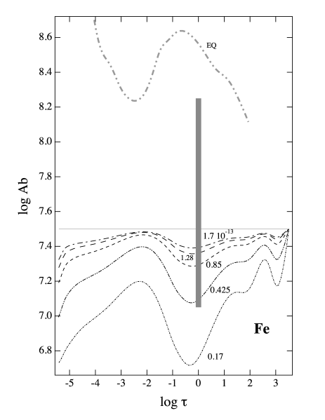
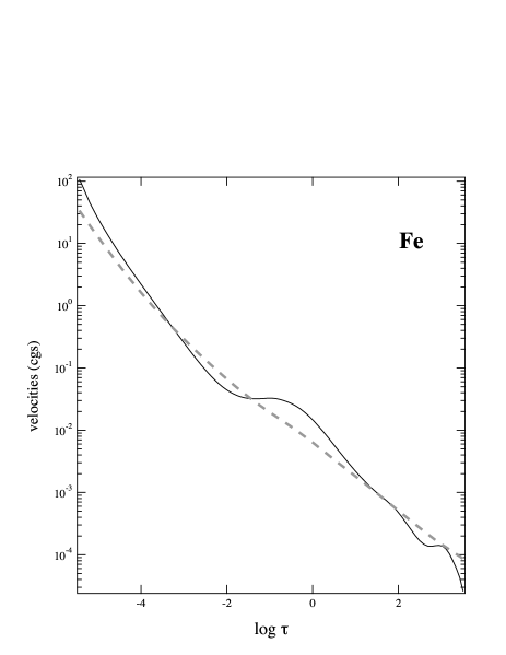
Fig. 3 and 4, present the stationary solutions for Fe (same mass-loss rates as for the Mg results). This time, the diffusion velocity is always positive and in closer competition with the wind velocity.

Figure 2: Mg diffusion and wind velocity respectively for the stationary solution. The solid line stands for positive diffusion velocities (upwards), the short-dashed line for negative velocities. The long-dashed line shows the wind velocity for a mass-loss rate of $0.425\,10^{-13}$ solar mass per year.

Figure 3: Same as Fig. 1a, for Fe.

Figure 4: Same as Fig. 2 for Fe.

3.2 Abundances of Mg and Fe in magnetic atmospheres

We have carried out a number of calculations for a magnetic atmosphere. However, these results – obtained for a plane-parallel model – have to be considered with extreme caution since one may reasonably suppose that in the magnetic case the stellar wind should be anisotropic (Babel, 1992). It is well known that the diffusion velocity does not directly depend on the vertical component of the magnetic field vector, but that it depends instead explicitly on the horizontal component of the field. To illustrate the effect of a magnetic field, we have considered the case of a horizontal field of moderate strength (5 kG). We expect that the wind will be impeded by horizontal magnetic lines, similarly to what happens to the diffusion velocity (but certainly in a different way) since atoms are mostly ionised in our models. Establishing stationary solutions for Mg and Fe using the same model as in the previous section, we therefore adopted the lowest mass-loss rate ($0.17\,10^{-13}$) for which the solution converges. The results are shown in Fig. 5 and 6. It transpires that in the uppermost layers, stationary stratifications are very different from the non-magnetic ones; diffusion velocities display a completely different profile over a large part of the atmosphere.

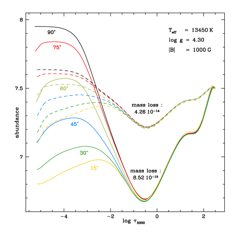
It is not without interest to have a look at the relative impact of magnetic fields and of mass loss on final stationary abundance distributions. Taking a stellar atmosphere with $T_{\rm eff}=13450\,$K and $\log g=4.30$ – similar to the one derived by Castelli et al. (2017) for HR 6000 – a field strength of 1000 G and mass loss rates of $8.5\,10^{-15}$ and $4.26\,10^{-14}$ respectively, we arrive at the angle-dependent stratifications shown in Fig. 7. As one would expect, the maximum difference in abundance between the horizontal and the vertical field case decreases with increasing mass loss. Whereas at $8.5\,10^{-15}$ abundances at $90^{\circ}$ are higher by about 1.15 dex than at $15^{\circ}$, this difference drops to about 0.55 dex when the mass loss is $4.26\,10^{-14}$. For field angles up to $45^{\circ}$, the solutions for $4.26\,10^{-14}$ lie consistently (by up to 0.5 dex) above those for $8.5\,10^{-15}$ throughout the atmosphere; when the angles exceed $60^{\circ}$, this is only true in those parts of the atmosphere where the magnetic field plays no role (below about $\log\tau=-0.5$).

At this point it is important to discuss an aspect of diffusion in magnetic stellar atmospheres that has received only the scantest attention in the past but whose repercussions on the comparison diffusion theory vs. empirical non-homogeneous abundances as derived from Zeeman Doppler mapping are of utmost relevance. We want to stress that all the exploratory modelling of the build-up of abundance stratifications in magnetic CP stars so far has employed a 1D approach, looking at the temporal evolution of the atmospheric structure in a “cylinder” of material isolated from its surroundings. In other words, only vertical velocities have been allowed, and the “cylinder” is assumed to stay in perfect pressure equilibrium with its surroundings all the time. On the other hand however, as Fig. 7 reveals, different field angles lead to different stratifications and to different atmospheric structure. From Fig. 9 of Stift & Leone (2017) one can deduce that angle-dependent stratifications will lead to angle-dependent horizontal pressure differences between adjacent “cylinders”. In the absence of an adequate stabilising force – e.g. a strong vertical magnetic field – horizontal pressure equilibrium will be established almost instantaneously, resulting in mixing between the “cylinders”. The problem has suddenly become 3D, even in the simple case of a centred dipole geometry. Although in a first approximation such mixing occurs only horizontally, independently for each geometric height in the atmosphere, it is clear that the resulting density, pressure and temperature structures of the individual “cylinders” will not in general ensure hydrostatic equilibrium. Relaxing to hydrostatic equilibrium in each cylinder should again entail deviations from horizontal pressure equilibrium. Whereas a magnetic star should adapt to the abundance-buildup in the shortest of times, the problem gets highly complex for any kind of numerical approach. Any realistic 3D modelling of atomic diffusion in strongly magnetic CP stars will have to deal with this additional challenge.

How does Zeeman Doppler mapping enter this discussion? Virtually every single abundance map in the literature has been derived under the assumption that the horizontal distribution of the chemical elements may be non-homogeneous but that all abundances, wherever on the stellar surface, have to be unstratified, i.e. constant from top to bottom of the atmosphere. In addition, in order to constrain the solutions to this ill-posed 2D inversion problem, people have mostly resorted to regularisation functions which look for the smoothest possible map. This approach is at variance with basic stellar astrophysics: Fig. 9 of Stift & Leone (2017) makes it abundantly clear that unstratified but horizontally non-homogeneous abundances structures cannot be in horizontal pressure equilibrium, independently of the approximations used in time-dependent atomic diffusion modelling. An approach by Rusomarov (2016) for 3D abundance mapping with the help of step-like abundance profiles that vary with position on the star also fails to reflect these and other (astro-)physical facts. The local profile in Rusomarov’s thesis is defined by the abundance in the high atmospheric layers $\epsilon_{up}$, the abundance deep in the atmosphere $\epsilon_{lo}$, the position $d$ of the transition region and its width $\delta$ where the abundance changes between $\epsilon_{up}$ and $\epsilon_{lo}$ (see his Fig. 2.3). Numerical models have established a bewildering multitude of vertical abundance profiles that frequently bear little resemblance to a step function as e.g. shown in Fig. 7. The position $d$ of the transition region always changes with magnetic field strength, the optical depth where the abundance reaches its maximum depends on the field angle. the spread in $|\epsilon_{up}-\epsilon_{lo}|$ is a function of field strength and field angle. Rusomarov’s regularisation function minimises all conceivable differences, i.e. between the horizontal gradients of the widths $\delta$, of the positions $d$, of the upper abundances $\epsilon_{up}$, and of the lower abundances $\epsilon_{lo}$. Additionally, the spread in $|\epsilon_{up}-\epsilon_{lo}|$ has to be minimum (see his formula 2.16), but all this is at variance with what we know about atomic diffusion in magnetic stellar atmospheres. There is no known/feasible physical mechanism that would lead to the kind of stratification plotted in Figs. 4 and 8 of Rusomarov et al. (2016).

To put it succinctly, neither are there empirical abundance stratifications of strongly magnetic CP stars available that could be confronted with theoretical results, nor is theory presently capable of treating the full 3D nature of diffusion in these stars. When it comes to real stars, in the present study we therefore prefer to stick to those which are non-magnetic or only weakly magnetic.

Figure 5: Stationary solutions in the same atmospheric model as for Fig. 1, but with a horizontal magnetic field of 5 kG (solid lines for Mg, dashed ones for Fe). The mass-loss rate is $0.17\,10^{-13}$, the smallest one for which the solution converges. The dashed light-grey line gives the Fe stationary solution, the solar abundance is plotted in dark-grey.

Figure 6: Diffusion velocities of Mg (thin black lines) and Fe (heavy black lines) for the stationary solutions of Fig. 5, and wind ($\rm{V_{w}}$) velocity (grey dashed line).

Figure 7: Fe abundance profiles as a function of optical depth, angle, and mass loss in an atmosphere with $T_{\rm eff}=13450$ K and $\log g=4.30$. A magnetic field strength of $|B|=1000$ G is assumed at angles $15^{\circ},30^{\circ},45^{\circ},60^{\circ},75^{\circ},90^{\circ}$ relative to the surface normal. Full lines refer to a mass-loss rate of $8.5\,10^{-15}$ solar mass per year, dashed lines to $4.26\,10^{-14}$ solar mass per year.

4 The case of HD 53929

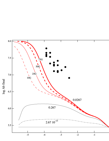
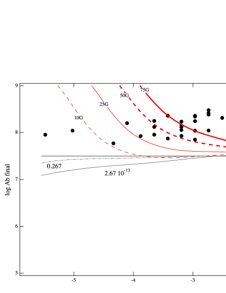
Recently, Ndiaye et al. (2018) have published an abundance analysis of 2 HgMn stars (HD 53929 and HD 63975). These authors found well marked abundance stratifications of phosphorus, and slight iron overabundances with very moderate abundance gradients. Both stars exhibit similar trends in the respective P and Fe abundance stratifications. We decided to apply our time-dependent atomic diffusion modelling to one of these stars. We have chosen HD 53929 which seems a less evolved main sequence star than HD 63975, thus a more typical HgMn star. According to Ndiaye et al. (2018), the atmospheric parameters are $T_{\rm{eff}}\approx 12750$ K and $\log{g}\approx 3.7$. The empirical abundance stratifications of P and Fe are shown in Fig. 8 and 9 respectively (filled black circles); we have used the same axis scales as in their paper.

The curves plotted in Fig. 8 and 9 correspond to the stationary solutions of our numerical simulations for various magnetic and mass-loss parameters. In these calculations, P and Fe are allowed to diffuse simultaneously, the atmospheric models being kept self-consistent by recomputing them with the actual abundances of both P and Fe at each time step – as we did previously for Mg and Fe (Sec. 2.1). The other elements are assumed to retain their solar ratios relative to hydrogen.

We first considered the non-magnetic case with various values of the mass-loss rate. The lowest mass-loss rate ($0.267\,10^{-13}$) differs from the lowest one of the model used in Sec. 3 (for non magnetic case) because of the higher effective temperature and lower gravity of HD 53929. The highest mass-loss we show here is 10 time larger. For both elements, the stationary solutions are far from the stratifications determined by Ndiaye et al. (2018). In particular, in high layers P remains marginally overabundant, Fe depleted. This may be explained by the fact that radiative accelerations largely exceed gravity in these layers, helping P and Fe to escape the star. To impede this escape one must assume a horizontal magnetic field. This magnetic field however has to be weak enough (or not well structured on a large scale) to be compatible with the lack of detection in HgMn stars (see the discussion in Sec. 5). In our calculations we have adopted weak horizontal fields in the range from 10 G to 75 G and the lowest mass-loss rate that yields stable stationary solutions (see Sec. 3.2). This mass-loss rate of $0.0267\,10^{-13}$ solar mass per year is small enough in our opinion to be assimilated to the zero mass-loss case. Results are shown in Fig. 8 and 9, the curves labelled with the magnetic field strength. Since the diffusion velocity drops drastically in higher layers due to the horizontal field, elements cannot easily escape the atmosphere but accumulate in these layers. The stronger the field, the closer the phosphorus stratification gets to those empirically determined from observations. The situation is less convincing for the iron stratification profile; the calculated overabundances however are now closer to the empirical values.

Figure 8: Stratification of P in the atmosphere of HD 53929. The filled circles show the abundances empirically determined by Ndiaye et al. (2018) from observations. The solid grey line is the solar abundance, the thin solid and dash-dot-dot curves are our stationary non-magnetic solutions for respective mass-loss rates of 2.67 and 0.267$\,10^{-13}$ solar mass per year. The group of red curves labelled 10 G, 25 G, 50 G, and 75 G are the solutions obtained by assuming a weak horizontal magnetic field, and for the lowest mass-loss that ensures convergence of this model (0.0267$\,10^{-13}$).

Figure 9: Same as Fig. 8 for Fe.

5 Discussion

5.1 Abundance of Mg in HgMn stars: a mass-loss rate gauge

As stressed in Sec. 3.1, Mg is an interesting element for constraining models, since it is observed moderately underabundant in HgMn stars whereas it should be strongly underabundant (by several orders of magnitude!) according to numerical simulations with atomic diffusion acting alone – no mass-loss – in non-magnetic atmospheres. From our results shown in Fig. 1 it appears that adding mass-loss to atomic diffusion may explain observed abundances. These abundances have been taken from the compilation of Ghazaryan & Alecian (2016) and are indicated by the vertical thick grey bar at $\log\tau=0.0$ in Fig. 1a. It turns out that the stationary solutions for Mg are very sensitive to the mass-loss rate adopted in the simulations. For the $T_{\rm{eff}}=12000$ K, $\log{g}=4.0$ model, and among the five different mass-loss rates we have considered, 0.425$\,10^{-13}$ solar mass per year yields the stationary solution best in accord with the observed abundances of Mg. The same mass-loss leads to stationary solutions for Fe compatible with the observed abundances. Of course we cannot and do not claim that the mass-loss rate that has to be adopted for this model should be exactly 0.425$\,10^{-13}$ solar mass per year. It seems clear however, that mass-loss rates of about 0.17$\,10^{-13}$ and lower are incompatible with the observed abundances.

Since Mg is only weakly supported by radiative acceleration at solar abundance (the radiative acceleration becomes lower than $-g$ for $\log\tau>{-4}$), the depletion of Mg is due to gravitational settling throughout the major part of the atmosphere, including deep layers where the diffusion velocity is no longer sensitive to magnetic fields. This means that even in the presence of a strong horizontal magnetic field, depletion of Mg will occur in deep layers; this is confirmed by observations which show that Mg is often depleted in magnetic ApBp stars. We are therefore inclined to consider magnesium a very good mass-loss indicator in hot CP stars.

5.2 The case of Fe

The vertical thick grey bar at $\log\tau=0.0$   in Fig. 3 marks the range of observed iron abundances in the HgMn stars considered in Fig. 1a. We can see that the abundances of Fe range go from -0.5  dex below to about +0.8 dex above the solar value. According to our results, the lowest mass-loss rate of 0.17$\,10^{-13}$ may be excluded, but all the others (including 0.425$\,10^{-13}$) are found compatible with observations. Whatever the overabundance, to obtain it one has to assume the presence of horizontal magnetic fields, even though they might be weak ones, as in the case of HD 53929 (see also Fig. 5).

5.3 Confronting time-dependent models with abundance stratifications deduced from observations

We have considered in detail the case of HD 53929, establishing stationary solutions for P and Fe. During the calculation of the build-up of the abundance stratifications, the atmospheric structure had to adapt continuously; effective temperature and gravity taken from Ndiaye et al. (2018) were kept constant. Our results for phosphorus are rather satisfactory since the abundance gradient of P is very close to the one determined empirically by these authors. Our best solution (with a horizontal magnetic field of 75 G) lies by about 0.5 dex below the empirical stratification, which is not really troubling, given the overabundance of 2.5 dex. Notice that the results shown in Fig. 8 for P may be compared to the stratification found by Catanzaro et al. (2016). These authors have found a deeper stratification of P in a HgMn star (HD 49606) with effective temperature and gravity not very different from HD 53929. In their work P is more enhanced than in our result, but the abundance gradient is compatible with the one we have found for P for $\log\tau>-2.0$. At this depth, according to our calculations, the stratification does not depend directly on a possible magnetic field.

Results are less satisfactory for Fe for which we find decreasing abundances with increasing depth, whereas a weak increase in abundance has been found by Ndiaye et al. (2018). The values of the predicted Fe overabundances are, however, quite consistent with the observational values. Please note at this point that Ndiaye et al. (2018) do not consider horizontal inhomogeneities in their abundance analysis but only vertical ones, whereas we implicitly assume that horizontal inhomogeneities exist, as soon as magnetic fields are present.

We want to point out an important aspect of our results, viz. that the best solutions require the existence of a weak horizontal magnetic field. Mass-loss does not seem to be the determining parameter for both P and Fe, which is at variance to what we find for Mg (Sec. 3.1 and 5.1). The question arises whether the field strengths in the calculations for HgMn stars can be considered compatible with the observations? Alecian (2012, 2013) has discussed the consequences of assuming weak magnetic fields in HgMn stars. He suggested that a weak magnetic field helps in explaining the presence of spots detected in some HgMn stars for elements like Nd, Pt, Hg and a few others (Adelman et al., 2002; Kochukhov et al., 2005; Hubrig et al., 2006), without contradicting the “canonical” diffusion model in which metals with high solar abundances should stratify in an isotropic way deeper in the atmosphere. From our present results we see that a weak magnetic field could also help in understanding abundance stratification of metals like phosphorus, perhaps also iron. The existence of such weak fields presently remains a hypothesis which needs confirmation by observations.

6 Conclusion

We have extended the applicability of our 1D numerical models of magnetic and non-magnetic CP star atmospheres by adding a mass-loss to atomic diffusion processes. In our calculations, the mass-loss rate is a free parameter that translates into a mass flow (or wind) with a given constant flux with respect to the depth. Mass-loss rates of around $5.0\,10^{-14}$ solar mass per year – already considered for AmFm stars by Alecian (1996) and Vick et al. (2010) – have been explored. Our results confirm that abundance stratifications due to atomic diffusion are indeed very sensitive to the mass-loss rate. We have shown that for a model atmosphere with $T_{\rm{eff}}=12000$ K and $\log{g}=4.0$, Mg will be extremely depleted in the absence of mass-loss, but actually Mg is found only mildly underabundant in HgMn stars. Such mild underabundances in our numerical simulations can only be achieved by assuming a mass-loss rate very close to $4.25\,10^{-14}$ solar mass per year, a rate that is also compatible with the observed abundances of Fe in the same class of stars. We propose to take Mg abundances in HgMn star as a kind of gauge for measuring the mass-loss rates of these stars. For the near future we are planning to explore models of various effective temperatures and gravities in order to find out how mass-loss rates might depend on stellar fundamental parameters.

We have also compared our numerical models to empirical abundance stratifications deduced from observations of real stars. For this purpose we have chosen the results of Ndiaye et al. (2018) obtained for P and Fe in the HgMn star HD 53929. The result for the stratification of P is found rather satisfactory, but only if a weak (75 G) horizontal magnetic field is accompanied by a very small mass-loss rate. This conclusion must not be generalised; we do not claim that fields of similar strength exist in all HgMn stars.

Many more numerical simulations have to be compared to empirical stratifications in order to get a more complete picture of the interplay of mass-loss and weak magnetic fields but there can be little doubt that mass-loss is an essential ingredient to diffusion models of CP stars.

References

- Adelman et al. (2002) Adelman S. J., Gulliver A. F., Kochukhov O. P., Ryabchikova T. A., 2002, ApJ, 575, 449
- Alecian (1986) Alecian G., 1986, A&A, 168, 204
- Alecian (1996) Alecian G., 1996, A&A, 310, 872
- Alecian (2012) Alecian G., 2012, in Shibahashi H., Takata M., Lynas-Gray A. E., eds, Astronomical Society of the Pacific Conference Series Vol. 462, Progress in Solar/Stellar Physics with Helio- and Asteroseismology. p. 80
- Alecian (2013) Alecian G., 2013, in Shibahashi H., Lynas-Gray A. E., eds, Astronomical Society of the Pacific Conference Series Vol. 479, Progress in Physics of the Sun and Stars: A New Era in Helio- and Asteroseismology. p. 35
- Alecian (2015) Alecian G., 2015, MNRAS, 454, 3143
- Alecian & Michaud (1981) Alecian G., Michaud G., 1981, ApJ, 245, 226
- Alecian & Stift (2004) Alecian G., Stift M. J., 2004, A&A, 416, 703
- Alecian & Stift (2017) Alecian G., Stift M. J., 2017, MNRAS, 468, 1023
- Alecian et al. (2011) Alecian G., Stift M. J., Dorfi E. A., 2011, MNRAS, 418, 986
- Babel (1992) Babel J., 1992, A&A, 258, 449
- Babel & Montmerle (1997) Babel J., Montmerle T., 1997, A&A, 323, 121
- Bischof (2005) Bischof K. M., 2005, Memorie della Societa Astronomica Italiana Supplementi, 8, 64
- Castelli et al. (2017) Castelli F., Cowley C. R., Ayres T. R., Catanzaro G., Leone F., 2017, A&A, 601, A119
- Catanzaro et al. (2016) Catanzaro G., Giarrusso M., Leone F., Munari M., Scalia C., Sparacello E., Scuderi S., 2016, MNRAS, 460, 1999
- Ghazaryan & Alecian (2016) Ghazaryan S., Alecian G., 2016, MNRAS, 460, 1912
- Hubrig et al. (2006) Hubrig S., González J. F., Savanov I., Schöller M., Ageorges N., Cowley C. R., Wolff B., 2006, MNRAS, 371, 1953
- Kochukhov & Ryabchikova (2018) Kochukhov O., Ryabchikova T. A., 2018, MNRAS, 474, 2787
- Kochukhov et al. (2005) Kochukhov O., Piskunov N., Sachkov M., Kudryavtsev D., 2005, A&A, 439, 1093
- Kurucz (2005) Kurucz R. L., 2005, Memorie della Societa Astronomica Italiana Supplementi, 8, 14
- Landstreet et al. (1998) Landstreet J. D., Dolez N., Vauclair S., 1998, A&A, 333, 977
- LeBlanc et al. (2009) LeBlanc F., Monin D., Hui-Bon-Hoa A., Hauschildt P. H., 2009, A&A, 495, 937
- Mathys & Hubrig (1995) Mathys G., Hubrig S., 1995, A&A, 293, 810
- Michaud (1970) Michaud G., 1970, ApJ, 160, 641
- Michaud et al. (1983) Michaud G., Tarasick D., Charland Y., Pelletier C., 1983, ApJ, 269, 239
- Michaud et al. (2015) Michaud G., Alecian G., Richer J., 2015, Atomic Diffusion in Stars, Astronomy and Astrophysics Library, Springer International Publishing, Switzerland., doi:10.1007/978-3-319-19854-5.
- Ndiaye et al. (2018) Ndiaye M. L., LeBlanc F., Khalack V., 2018, MNRAS, 477, 3390
- Oskinova et al. (2011) Oskinova L. M., Todt H., Ignace R., Brown J. C., Cassinelli J. P., Hamann W.-R., 2011, MNRAS, 416, 1456
- Rusomarov (2016) Rusomarov N., 2016, PhD dissertation, retrieved from http://urn.kb.se/resolve?urn=urn:nbn:se:uu:diva-278535
- Rusomarov et al. (2016) Rusomarov N., Kochukhov O., Ryabchikova T., 2016, Retrieved from http://urn.kb.se/resolve?urn=urn:nbn:se:uu:diva-278534
- Schaller et al. (1992) Schaller G., Schaerer D., Meynet G., Maeder A., 1992, A&AS, 96, 269
- Smith & Dworetsky (1993) Smith K. C., Dworetsky M. M., 1993, A&A, 274, 335
- Stift & Alecian (2012) Stift M. J., Alecian G., 2012, MNRAS, 425, 2715
- Stift & Alecian (2016) Stift M. J., Alecian G., 2016, MNRAS, 457, 74
- Stift & Leone (2017) Stift M. J., Leone F., 2017, ApJ, 834, 24
- Stift et al. (2013) Stift M. J., Alecian G., Dorfi E. A., 2013, in Alecian G., Lebreton Y., Richard O., Vauclair G., eds, EAS Publications Series Vol. 63, EAS Publications Series. pp 227–232, doi:10.1051/eas/1363026
- Vauclair (1975) Vauclair S., 1975, A&A, 45, 233
- Vick et al. (2010) Vick M., Michaud G., Richer J., Richard O., 2010, A&A, 521, A62