One-stage explicit trigonometric integrators
for effectively solving quasilinear wave equations

Abstract

In this paper, one-stage explicit trigonometric integrators for solving quasilinear wave equations are formulated and studied. For solving wave equations, we first introduce trigonometric integrators as the semidiscretization in time and then consider a spectral Galerkin method for the discretization in space. We show that one-stage explicit trigonometric integrators in time have second-order convergence and the result is also true for the fully discrete scheme without requiring any CFL-type coupling of the discretization parameters. The results are proved by using energy techniques, which are widely applied in the numerical analysis of methods for partial differential equations.

Keywords: quasilinear wave equations, trigonometric integrators, second-order convergence, energy technique

MSC: 65M15, 65P10, 65L70, 65M20.

1 Introduction

In this paper, we are devoted to the numerical methods for effectively solving quasilinear wave equations of the form (see [10])

$$\begin{array}[c]{ll}\partial_{t}^{2}u=\partial_{x}^{2}u-u+\kappa a(u)\partial_{x}^{2}u+\kappa g(u,\partial_{x}u),\quad x\in{\mathbb{T}}={\mathbb{R}}/(2\pi{\mathbb{Z}}),\ t\in[0,T],\end{array}$$ (1)

with the smooth and real-valued functions $g$ and $a$ satisfying $g(0,0)=a(0)=0.$ In this paper, the strength of the nonlinearities is emphasized by the real-valued parameter $\kappa$ and we consider $\kappa$ to be small $0<\kappa\ll 1$ such that the nonlinearities are small. The initial values at time $t=0$ are assumed to be

$$\begin{array}[c]{ll}u(\cdot,0)=u_{0},\ \ \ \partial_{t}u(\cdot,0)=\dot{u}_{0}\end{array}$$ (2)

and the boundary conditions are $2\pi$-periodic in one space dimension. It is noted that the solutions of (1) are assumed to be real-valued in this paper.

It is well known that quasilinear wave equations occur in a variety of applications such as elastodynamics and general relativity (see, e.g. [7, 17, 23]). These equations have also been used to describe many problems which appear in elasticity, fluid mechanics and general relativity (see, e.g. [18]). Compared with many publications about the analysis of these equations ([2, 7, 17, 18, 23, 28]), there is much less work devoted to the numerical solutions and numerical analysis for quasilinear wave equations.

These equations with small $\kappa$ have been extensively studied by [3, 4, 8, 13]. However, in the numerical discretization of (1), the quasilinear term $\kappa a(u)\partial_{x}^{2}u$ is the principal difficulty, which needs to be dealt with carefully. In order to effectively solve (1), some implicit and semi-implicit methods of Runge-Kutta type for semi-discretization in time were proposed and researched recently in [16, 19] . More recently, the authors in [10] showed that a class of explicit exponential integrators given in [14, 15] can be used to numerically solve the quasilinear wave equation (1) with two regimes of $\kappa$ by using the energy technique with a modified discrete energy.

In order to effectively solve the quasilinear wave equation (1), a class of one-stage explicit trigonometric integrators will be rigorously studied in this paper. We prove second-order convergence not only for the methods in time but also for the fully discrete schemes. These trigonometric integrators were firstly developed in [34] for solving highly oscillatory ODEs and we refer the reader to [25, 27, 29, 30, 33] for further researches. Meanwhile, this kind of methods has been applied to wave equations in the semilinear case (see, e.g. [20, 21, 26, 31, 32]). However, these methods have not been researched for quasilinear wave equations, which motivates this paper.

The main contribution of this work is to show the error bounds of trigonometric integrators for quasilinear wave equations. In contrast to the analysis in [10], we do not use a modified discrete energy in this paper and just take the simple and normal energy technique, which is widely used in the numerical analysis of partial differential equations (see, e.g. [1, 5, 6, 9, 11, 12, 16, 19, 22, 27]). The paper is displayed as follows. In Section 2 trigonometric integrators for the discretization in time and full-discrete trigonometricintegrators are introduced. The main results of this paper are presented in Section 3 and a numerical experiment is carried out to show the numerical behaviour and support the theoretical analysis. In Section 4 we prove the error bounds for trigonometric integrators in time. Section 5 is devoted to the proof of error bounds for full-discrete trigonometric integrators. For one of the trigonometric integrators, a simple proof for the error bounds is presented in Section 6 by establishing a relationship between this integrator and a trigonometric integrator researched in [10]. Finally, in Section 7 we include the conclusions of this paper.

2 Trigonometric integrators

In this paper, we will use the following notations and properties, which have been used in [10].

• Denote by $H^{s}=H^{s}({\mathbb{T}})$ with $s\geq 0$ the usual Sobolev space and its norm $\left\|\cdot\right\|_{s}$ is given by

  $$\left\|v\right\|_{s}^{2}=\sum\limits_{j\in{\mathbb{Z}}}\langle j\rangle^{2s}|\hat{v}_{j}|^{2}\quad\textmd{for}\quad v(x)=\sum\limits_{j\in{\mathbb{Z}}}\hat{v}_{j}\mathrm{e}^{\mathrm{i}jx},$$ (3)

  where the weights $\langle j\rangle$ for $j\in{\mathbb{Z}}$ are defined $\langle j\rangle=\sqrt{j^{2}+1}.$

• The corresponding scalar product is defined by $\langle\cdot\rangle_{s}$:

  $$\langle v,w\rangle_{s}=\sum\limits_{j\in{\mathbb{Z}}}\langle j\rangle^{2s}\bar{\hat{v}}_{j}\hat{w}_{j}\quad\textmd{for}\quad v(x)=\sum\limits_{j\in{\mathbb{Z}}}\hat{v}_{j}\mathrm{e}^{\mathrm{i}jx},\ \ \quad w(x)=\sum\limits_{j\in{\mathbb{Z}}}\hat{w}_{j}\mathrm{e}^{\mathrm{i}jx}.$$

• The solutions $(u(\cdot,t),\partial_{t}u(\cdot,t))$ of the quasilinear wave equation (1) are studied in the spaces $H^{s+1}\times H^{s}$ with the norm

  $${\left|\kern-1.07639pt\left|\kern-1.07639pt\left|(u,\dot{u})\right|\kern-1.07639pt\right|\kern-1.07639pt\right|}_{s}=(\left\|u\right\|^{2}_{s+1}+\left\|\dot{u}\right\|^{2}_{s})^{1/2}.$$

• The following classical estimates in Sobolev spaces will be used in this paper for $s>\frac{1}{2}$ (see Chapter 13 of [24]):

  $$\left\|uv\right\|_{0}\leq C_{s}\left\|u\right\|_{0}\left\|v\right\|_{s},\qquad\left\|uv\right\|_{s}\leq C_{s}\left\|u\right\|_{s}\left\|v\right\|_{s}.$$ (4)

• Another classical estimates for any smooth function $G$ with $G(0)=0$ are (see Chapter 13 of [24])

  $$\left\|G(u)\right\|_{s}\leq\Lambda_{s}(\left\|u\right\|_{s})\left\|u\right\|_{s},\quad\left\|G(u)-G(v)\right\|_{s}\leq\Lambda_{s}(\left\|u\right\|_{s}+\left\|v\right\|_{s})\left\|u-v\right\|_{s},$$ (5)

  where $\Lambda_{s}(\cdot)$ is a continuous nondecreasing function.

• It is noted that the norm and the scalar product have the following connection

  $$\left\|u\pm v\right\|_{1}^{2}=\left\|u\right\|_{1}^{2}+\left\|v\right\|_{1}^{2}\pm 2\langle u,v\rangle_{1}.$$ (6)

2.1 Methods for the discretization in time

By letting

$$f(u)=a(u)\partial_{x}^{2}u+g(u,\partial_{x}u),$$ (7)

and the linear operator

$$\Omega=\sqrt{-\partial_{x}^{2}+1},$$

the quasilinear wave equation (1) becomes

$$\partial_{t}^{2}u=-\Omega^{2}u+\kappa f(u).$$ (8)

In what follows, one-stage explicit trigonometric integrators are used for the discretization in time of (8).

Definition 2.1

(See [34].) For solving (8), we consider a one-stage explicit trigonometric integrator which is given by

$$\left\{\begin{array}[c]{ll}u_{n+c_{1}}&=\phi_{0}(c_{1}^{2}V)u_{n}+hc_{1}\phi_{1}(c_{1}^{2}V)\dot{u}_{n},\\ u_{n+1}&=\phi_{0}(V)u_{n}+h\phi_{1}(V)\dot{u}_{n}+\kappa h^{2}\bar{b}_{1}(V)f(u_{n+c_{1}}),\\ \dot{u}_{n+1}&=-h\Omega^{2}\phi_{1}(V)u_{n}+\phi_{0}(V)\dot{u}_{n}+\kappa h\textstyle b_{1}(V)f(u_{n+c_{1}}),\end{array}\right.$$ (9)

where $c_{1}\in[0,1]$ denotes a real constant and $h$ is the stepsize. The coefficients $b_{1}(V)$ and $\bar{b}_{1}(V)$ are operator-valued functions of $V\equiv h^{2}\Omega^{2}$, and further we define

$$\phi_{0}(V)=\cos(h\Omega),\qquad\phi_{1}(V)=\textmd{sinc}(h\Omega):=(h\Omega)^{-1}\sin(h\Omega).$$

From the symmetry conditions of trigonometric integrators given in [33], it follows that the integrator (9) is symmetric if and only if

$$c_{1}=1/2,\ \ \mathrm{sinc}(h\Omega)b_{1}(V)=(I+\cos(h\Omega))\bar{b}_{1}(V),$$ (10)

where $I$ is the identical operator. Under this condition, the trigonometric integrator (9) can be rewritten as

$$\left\{\begin{array}[c]{ll}u_{n+\frac{1}{2}}&=\cos(\frac{1}{2}h\Omega)u_{n}+\frac{1}{2}h\mathrm{sinc}(\frac{1}{2}h\Omega)\dot{u}_{n},\\ \dot{u}^{+}_{n}&=\dot{u}_{n}+h\kappa\mathrm{sinc}(h\Omega)^{-1}\bar{b}_{1}(V)f(u_{n+\frac{1}{2}}),\\ \left(\begin{array}[]{c}\Omega u_{n+1}\\ \dot{u}^{-}_{n+1}\\ \end{array}\right)&=\left(\begin{array}[]{cc}\cos(h\Omega)&\sin(h\Omega)\\ -\sin(h\Omega)&\cos(h\Omega)\\ \end{array}\right)\left(\begin{array}[]{c}\Omega u_{n}\\ \dot{u}^{+}_{n}\\ \end{array}\right),\\ \dot{u}_{n+1}&=\dot{u}^{-}_{n+1}+h\kappa\mathrm{sinc}(h\Omega)^{-1}\bar{b}_{1}(V)f(u_{n+\frac{1}{2}}).\end{array}\right.$$ (11)

We denote the numerical flow of this integrator by $\varphi_{h}$, i.e., $(u_{n+1},\dot{u}_{n+1})=\varphi_{h}(u_{n},\dot{u}_{n}).$

In this paper, the one-stage explicit trigonometric integrator (9) is considered under the following assumption.

Assumption 2.2

For the coefficient functions of the one-stage explicit trigonometric integrator (9), we require the symmetry condition (10) and assume that there exists a constant $c$ such that

$$\begin{array}[]{ll}|\xi\bar{b}_{1}(\xi^{2})|\leq c,&\quad|\xi^{2}\bar{b}_{1}(\xi^{2})|\leq c,\qquad\qquad\qquad|\bar{b}_{1}(\xi^{2})-\frac{1}{2}\mathrm{sinc}(\frac{1}{2}\xi)|\leq c\xi,\\ |\xi b_{1}(\xi^{2})|\leq c,&\quad|b_{1}(\xi^{2})-\cos(\frac{1}{2}\xi)|\leq c\xi^{2},\ \ \ \ \ |\xi\mathrm{sinc}(\xi)^{-1}b_{1}(\xi^{2})|\leq c\end{array}$$ (12)

for all $\xi\geq 0$

2.2 Full-discrete methods

As the full discretization of (8), we consider the trigonometric integrators for the discretization in time and a spectral Galerkin method for the discretization in space (see, e.g. [10]).

Denote the space of trigonometric polynomials of degree $K$ by

$$\mathcal{V}^{K}=\Big{\{}\sum\limits_{j=-K}^{K}\hat{v}_{j}\mathrm{e}^{\mathrm{i}jx}:\hat{v}_{j}\in\mathbb{C}\Big{\}}$$

and the $L^{2}$-orthogonal projection onto this ansatz space by

$$\mathcal{P}^{K}(v)=\sum\limits_{j=-K}^{K}\hat{v}_{j}\mathrm{e}^{\mathrm{i}jx}\quad\textmd{for}\quad v=\sum\limits_{j=-\infty}^{\infty}\hat{v}_{j}\mathrm{e}^{\mathrm{i}jx}\in L^{2}.$$ (13)

Then the nonlinearity $f(u)$ in the method in time (9) is considered to be replaced by the following new nonlinearity

$$\hat{f}^{K}(u)=\mathcal{P}^{K}(f^{K}(u)),$$ (14)

where

$$f^{K}(u)=a^{K}(u)\partial_{x}^{2}u+g^{K}(u,\partial_{x}u)\quad\textmd{with}\quad a^{K}=\mathcal{I}^{K}\circ a,\ g^{K}=\mathcal{I}^{K}\circ g.$$

Here the notation $\mathcal{I}^{K}$ is used to describe the trigonometric interpolation in the space $\mathcal{V}^{K}$.

We are now in the position to present the fully discrete trigonometric integrator

$$\begin{array}[c]{ll}u^{K}_{n+\frac{1}{2}}&=\cos(\frac{1}{2}h\Omega)u^{K}_{n}+\frac{1}{2}h\mathrm{sinc}(\frac{1}{2}h\Omega)\dot{u}^{K}_{n},\\ u^{K}_{n+1}&=\cos(h\Omega)u^{K}_{n}+h\mathrm{sinc}(h\Omega)\dot{u}^{K}_{n}+\kappa h^{2}\bar{b}_{1}(V)\hat{f}^{K}(u^{K}_{n+\frac{1}{2}}),\\ \dot{u}^{K}_{n+1}&=-\Omega\sin(h\Omega)u^{K}_{n}+\cos(h\Omega)\dot{u}^{K}_{n}+\kappa h\textstyle b_{1}(V)\hat{f}^{K}(u^{K}_{n+\frac{1}{2}}),\end{array}$$ (15)

where $u^{K}_{n}\in\mathcal{V}^{K}$ and $\dot{u}^{K}_{n}\in\mathcal{V}^{K}$ are the numerical solutions of $u(\cdot,t_{n})$ and $\partial_{t}u(\cdot,t_{n})$ respectively. Moreover, the initial values $u_{0}$ and $\dot{u}_{0}$ of (2) are replaced by

$$u^{K}_{0}=\mathcal{P}^{K}(u_{0}),\qquad\dot{u}^{K}_{0}=\mathcal{P}^{K}(\dot{u}_{0}).$$

We denote the fully discrete integrator (15) as $(u^{K}_{n+1},\dot{u}^{K}_{n+1})=\varphi^{K}_{h}(u^{K}_{n},\dot{u}^{K}_{n}).$

Remark 2.3

It is noted that the nonlinearity $\hat{f}^{K}$ appearing in the fully discrete trigonometric integrator (15) can be computed efficiently by fast Fourier techniques (see [10]).

3 Main results and numerical test

In this section, the error bounds are presented not only for the methods in time but also for the fully discrete schemes. The exact solution $u(x,t)$ to (8) is required to satisfy the following assumption, which has been considered in [10].

Assumption 3.1

(See [10].) The exact solution $(u(\cdot,t),\partial_{t}u(\cdot,t))$ to (8) is assumed to be in $H^{5+s}\times H^{4+s}$ with

$${\left|\kern-1.07639pt\left|\kern-1.07639pt\left|(u(\cdot,t),\partial_{t}u(\cdot,t))\right|\kern-1.07639pt\right|\kern-1.07639pt\right|}_{4+s}\leq M\quad\textmd{for}\quad 0\leq t\leq T,$$ (16)

where $s\geq 0$ and $M>0$. Moreover, we assume that there are $0<\delta<1$ and $A_{0}\geq 0$ such that $1+\kappa a(u(\cdot,t))\leq\delta>0$ and $\kappa a(u(\cdot,t))\leq A_{0}$ for $0\leq t\leq T.$

Remark 3.2

The regularity assumption (16) on the exact solution was considered in [10] and it is true locally in time for initial values in $H^{5+s}\times H^{4+s}$ by local well-posedness theory (see [18, 23]).

3.1 Main results

Theorem 3.3

(Convergence for trigonometric integrators in time.) Assume that Assumption 2.2 holds for the coefficient functions of trigonometric integrators and Assumption 3.1 is true for the exact solution $(u(\cdot,t),\partial_{t}u(\cdot,t))$ with $s=0$. Then there is a constant $h_{0}>0$ such that for $0<\kappa\ll 1$ and for all $\kappa\lesssim h<h_{0}$, the following convergence for the time-discrete trigonometric integrator $(u_{n},\dot{u}_{n})$ (9) in $H^{2}\times H^{1}$ holds

$${\left|\kern-1.07639pt\left|\kern-1.07639pt\left|(u_{n},\dot{u}_{n})-(u(\cdot,t_{n}),\partial_{t}u(\cdot,t_{n}))\right|\kern-1.07639pt\right|\kern-1.07639pt\right|}_{1}\leq Ch^{2}\qquad\textmd{for}\qquad 0\leq t_{n}=nh\leq T,$$ (17)

where the constant $C$ depends on the smooth functions $a$ and $g$ in (1), the constant $c$ of Assumption 2.2, the constant $M$ from Assumption 3.1, but is independent of the time step-size $h$ and the final time $T$.

Theorem 3.4

(Convergence for full-discrete trigonometric integrators.) Under the conditions in Theorem 3.3 but with a fixed $s\geq 0$ instead of $s=0$, there is $h_{0}>0$ such that for $0<\kappa\ll 1$ and for all $\kappa\lesssim h<h_{0}$, the convergence for the full-discrete trigonometric integrator $(u^{K}_{n},\dot{u}^{K}_{n})$ of (15) in $H^{2}\times H^{1}$ is

$${\left|\kern-1.07639pt\left|\kern-1.07639pt\left|(u^{K}_{n},\dot{u}^{K}_{n})-(u(\cdot,t_{n}),\partial_{t}u(\cdot,t_{n}))\right|\kern-1.07639pt\right|\kern-1.07639pt\right|}_{1}\leq Ch^{2}+CK^{-s-2}\qquad\textmd{for}\qquad 0\leq t_{n}=nh\leq T.$$ (18)

Theorem 3.5

(Convergence for a special trigonometric integrator.) For a special trigonometric integrator TI2 which is presented in Table 1 and does not satisfy the last requirement in Assumption 2.2, it has the global error bound (17) for TI2 in time and the global error bound (18) for the full-discrete TI2.

Remark 3.6

It is noted that this paper only considers one regime of $\kappa$ which is that $\kappa$ is small. The reason is that the bound (26) can be true only for this case. For the regime $1$ of $\kappa$, we can only obtain that

$$\left|\mathcal{R}(u_{n+1},v_{n+1},u_{n},v_{n})\right|\leq C_{M}h{\left|\kern-1.07639pt\left|\kern-1.07639pt\left|(u_{n}-v_{n},\dot{u}_{n}-\dot{v}_{n})\right|\kern-1.07639pt\right|\kern-1.07639pt\right|}_{1},$$

which is not sufficient for deriving the second-order convergence of the trigonometric integrators. For the convergence of the trigonometric integrators when applied to quasilinear wave equations with $\kappa=1$, the possible way to work is to use a modified energy instead of the normal energy techniques and we will study it in future.

3.2 Numerical test

As an example, we present three practical one-stage explicit trigonometric integrators and their coefficients are listed in Table 1.

$$\begin{array}[]{|c|c|c|c|c|c|c|c|}\hline\cr\text{Methods}&c_{1}&\bar{b}_{1}(V)&b_{1}(V)\\ \hline\cr\text{TI1}&\frac{1}{2}&\frac{1}{2}{\phi^{3}_{1}(V/4)}&{\phi^{2}_{1}(V/4)\phi_{0}(V/4)}\cr\text{TI2}&\frac{1}{2}&\frac{1}{2}\phi_{1}(V)\phi_{1}(V/4)&\phi_{1}(V)\phi_{0}(V/4)\cr\text{TI3}&\frac{1}{2}&\frac{1}{2}\phi_{1}(V)\phi_{1}^{2}(V/4)&\phi_{1}(V)\phi_{1}(V/4)\phi_{0}(V/4)\cr\hline\cr\end{array}$$

Table 1: Three one-stage explicit trigonometric integrators.

It can be checked easily that these three integrators except TI2 satisfy all the requirements in Assumption 2.2. For the convergence of TI2, we will give another proof in Section 6 which does not rely on Assumption 2.2. For comparison, we choose a trigonometric integrator (formula (15) with $c=2$ of [10]) and denote it as NTI.

We consider the quasilinear wave equation (1) with $a(u)=u$ and $g(u,\partial_{x}u)=(\partial_{x}u)^{2}+\kappa u^{3},$ which has been studied in [4, 10]. The initial values are chosen as

$$u(x,0)=\sum\limits_{j\in{\mathbb{Z}}}\frac{1}{\sqrt{1+\left|j\right|^{11+\frac{1}{50}}}}e^{\mathrm{i}jx},\ \ \ \partial_{t}u(x,0)=\sum\limits_{j\in{\mathbb{Z}}}\frac{1}{\sqrt{1+\left|j\right|^{9+\frac{1}{50}}}}e^{\mathrm{i}jx}.$$

It is noted that these initial values are not in $H^{5+\sigma}\times H^{4+\sigma}$ for $\sigma\geq 1/100$ but they are in $H^{5}\times H^{4}$. Moreover, the regularity assumption (16) with $s=0$ is true for the initial values. We solve this problem in $[0,T]$ with $\kappa=1/100$ and the setpsizes $h=\frac{1}{2^{j}}$ for $j=1,2,\cdots,11$. The errors in $H^{2}\times H^{1}$ of these three trigonometric integrators are plotted in Figures 1-3. The observed convergence of these methods are two, which supports the results of Theorems 3.3-3.4. Moreover, it follows from the results that the trigonometric integrators behave better than the integrator NTI.

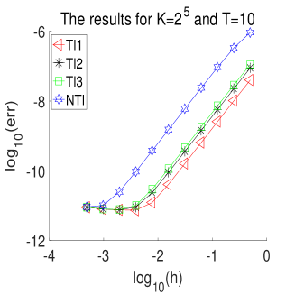
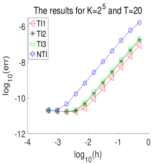
Figure 1: Results for $K=2^{5}$. The logarithm of the errors against the logarithm of stepsizes.

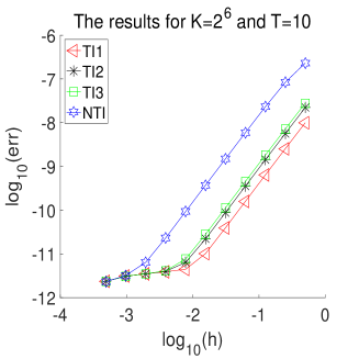
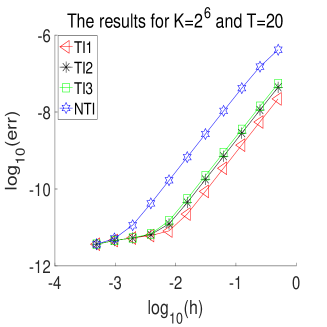
Figure 2: Results for $K=2^{6}$. The logarithm of the errors against the logarithm of stepsizes.

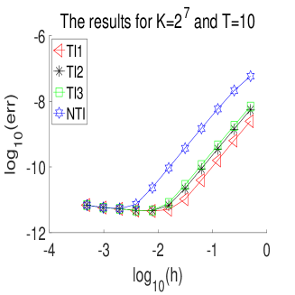
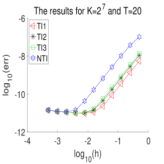
Figure 3: Results for $K=2^{7}$. The logarithm of the errors against the logarithm of stepsizes.

4 Proof of error bounds for trigonometric integrators in time

Theorem 3.3 will be proved in this section. Following [10] and in order to present this paper as a concise proof of concept, we limit ourselves to the exemplary case $g\equiv 0$ in (1), i.e.,

$$f(u)=a(u)\partial_{x}^{2}u.$$ (19)

Since the most critical part of the nonlinearity in (1) is the quasilinear term $a(u)\partial_{x}^{2}u$, it is straightforward to extend the proof to nonzero $g$, which will be noted after each step of the proof.

We remark that in the proof, denote by $C$ a generic constant that may depend on $a$, the order of the Sobolev space under consideration and on the constants in Assumptions 2.2 and 3.1. Denote by lower indices the additional dependencies of $C$, e.g., $C_{M}$ with $M$ from (16).

4.1 Bounds for a single time step

By the estimates (4)-(5) and the smoothness of $a$, some fundamental properties of the nonlinearity $f$ in (19) are obtained, which have been given in [10] and will be used in the proof.

Lemma 4.1

(See [10]) For the nonlinearity $f$ in (19), it is true that

$$\left\|f(u)\right\|_{s}\leq\Lambda_{s}(\left\|u\right\|_{\sigma})\left\|u\right\|_{\sigma}\left\|u\right\|_{s+2}\quad\textmd{with}\quad\sigma=\max(s,1),$$ (20)

and the Lipschitz property

$$\left\|f(u)-f(v)\right\|_{s}\leq\Lambda_{s}(\left\|u\right\|_{s+2}+\left\|v\right\|_{s+2})(\left\|u\right\|_{s+2}+\left\|v\right\|_{s+2})\left\|u-v\right\|_{s+2},$$ (21)

where $s\geq 0$, $u,v\in H^{s+2}$, and $\Lambda_{s}(\cdot)$ is a continuous non-decreasing function.

The following lemma shows that the time-discrete trigonometric integrator $\varphi_{h}$ given by (11) maps $H^{s+1}\times H^{s}$ to itself for $s\geq 1$.

Lemma 4.2

(Bounds for a single time step.) Let $s\geq 1$ and it is assumed that Assumption 2.2 holds. If a time-discrete trigonometric integrator $(u_{n},\dot{u}_{n})\in H^{s+1}\times H^{s}$ satisfies ${\left|\kern-1.07639pt\left|\kern-1.07639pt\left|(u_{n},\dot{u}_{n})\right|\kern-1.07639pt\right|\kern-1.07639pt\right|}_{s}\leq M,$ then it is true that

$$\left\|u_{n+\frac{1}{2}}\right\|_{s+1}\leq C_{M}$$

and $(u_{n+1},\dot{u}_{n+1})\in H^{s+1}\times H^{s}$ with

$${\left|\kern-1.07639pt\left|\kern-1.07639pt\left|(u_{n+1},\dot{u}_{n+1})\right|\kern-1.07639pt\right|\kern-1.07639pt\right|}_{s}\leq C_{M}.$$

Proof From the definition of the trigonometric integrator (9), it follows that

$$\begin{array}[c]{ll}\left\|u_{n+\frac{1}{2}}\right\|_{s+1}&\leq\left\|\cos\big{(}\frac{1}{2}h\Omega\big{)}u_{n}\right\|_{s+1}+\frac{1}{2}\left\|\Omega^{-1}\sin\big{(}\frac{1}{2}h\Omega\big{)}\dot{u}_{n}\right\|_{s+1}\\ &=\left\|\cos\big{(}\frac{1}{2}h\Omega\big{)}u_{n}\right\|_{s+1}+\frac{1}{2}\left\|\sin\big{(}\frac{1}{2}h\Omega\big{)}\dot{u}_{n}\right\|_{s}\leq C_{M}.\end{array}$$

Thus

$$\begin{array}[c]{ll}h^{2}\left\|\bar{b}_{1}(V)f(u_{n+\frac{1}{2}})\right\|_{s+1}&\leq\left\|\Omega^{-2}f(u_{n+\frac{1}{2}})\right\|_{s+1}=\left\|f(u_{n+\frac{1}{2}})\right\|_{s-1}\\ &\leq\Lambda_{s-1}\big{(}\left\|u_{n+\frac{1}{2}}\right\|_{s+1}\big{)}\left\|u_{n+\frac{1}{2}}\right\|^{2}_{s+1}\end{array}$$

is seen from the second formula in (12) and (20). In a similar way, by the fourth formula in (12) it arrives that

$$\begin{array}[c]{ll}h\left\|b_{1}(h\Omega)f(u_{n+\frac{1}{2}})\right\|_{s}&\leq\left\|\Omega^{-1}f(u_{n+\frac{1}{2}})\right\|_{s}=\left\|f(u_{n+\frac{1}{2}})\right\|_{s-1}\\ &\leq\Lambda_{s-1}\big{(}\left\|u_{n+\frac{1}{2}}\right\|_{s+1}\big{)}\left\|u_{n+\frac{1}{2}}\right\|^{2}_{s+1}.\end{array}$$

Therefore, considering the scheme of trigonometric integrator (9) again leads to

$$\begin{array}[c]{ll}\left\|u_{n+1}\right\|_{s+1}&\leq\left\|\cos(h\Omega)u_{n}\right\|_{s+1}+\left\|\Omega^{-1}\sin(h\Omega)\dot{u}_{n}\right\|_{s+1}+h^{2}\left\|\bar{b}_{1}(h\Omega)f(u_{n+\frac{1}{2}})\right\|_{s+1}\\ &\leq\left\|u_{n}\right\|_{s+1}+\left\|\dot{u}_{n}\right\|_{s}+\Lambda_{s-1}\big{(}\left\|u_{n+\frac{1}{2}}\right\|_{s+1}\big{)}\left\|u_{n+\frac{1}{2}}\right\|^{2}_{s+1}\end{array}$$

and

$$\begin{array}[c]{ll}\left\|\dot{u}_{n+1}\right\|_{s}&\leq\left\|\Omega\sin(h\Omega)u_{n}\right\|_{s}+\left\|\cos(h\Omega)\dot{u}_{n}\right\|_{s}+h\left\|b_{1}(h\Omega)f(u_{n+\frac{1}{2}})\right\|_{s}\\ &\leq\left\|u_{n}\right\|_{s+1}+\left\|\dot{u}_{n}\right\|_{s}+\Lambda_{s-1}\big{(}\left\|u_{n+\frac{1}{2}}\right\|_{s+1}\big{)}\left\|u_{n+\frac{1}{2}}\right\|^{2}_{s+1}.\end{array}$$

 $\Box{~{}}$

Remark 4.3

It is noted that from the proof, it follows that this lemma is still true for a nonzero $g$ in (1).

4.2 Stability

In this subsection, we will show the stability of trigonometric integrators. Before presenting the result, the following two lemmas are needed.

Lemma 4.4

Assume that Assumption 2.2 holds with constant $c$. For two time-discrete trigonometric numerical solutions $(u_{n},\dot{u}_{n})\in H^{s+1}\times H^{s}$ and $(v_{n},\dot{v}_{n})\in H^{s+1}\times H^{s}$ with $s\geq 0$, one has that

$$\begin{array}[c]{ll}{\left|\kern-1.07639pt\left|\kern-1.07639pt\left|(u_{n+1}-v_{n+1},\dot{u}_{n+1}-\dot{v}_{n+1})\right|\kern-1.07639pt\right|\kern-1.07639pt\right|}^{2}_{1}={\left|\kern-1.07639pt\left|\kern-1.07639pt\left|(u_{n}-v_{n},\dot{u}_{n}-\dot{v}_{n})\right|\kern-1.07639pt\right|\kern-1.07639pt\right|}^{2}_{1}+\kappa\mathcal{R}(u_{n+1},v_{n+1},u_{n},v_{n}),\end{array}$$

where the remainder is given by

$$\begin{array}[c]{ll}\mathcal{R}(u_{n+1},v_{n+1},u_{n},v_{n})\\ =\langle 2\mathrm{sinc}(h\Omega)^{-1}{b_{1}(V)}(u_{n+1}-u_{n}-v_{n+1}+v_{n}),f(u_{n+\frac{1}{2}})-f(v_{n+\frac{1}{2}})\rangle_{1}.\end{array}$$ (22)

Proof In this proof, we will use the following results

$$\begin{array}[c]{ll}h\mathrm{sinc}(h\Omega)\dot{u}_{n+1}=\cos(h\Omega)u_{n+1}+\kappa h^{2}\bar{b}_{1}(V)f(u_{n+\frac{1}{2}})-u_{n},\\ h\mathrm{sinc}(h\Omega)\dot{u}_{n}=-\cos(h\Omega)u_{n}-\kappa h^{2}\bar{b}_{1}(V)f(u_{n+\frac{1}{2}})+u_{n+1},\end{array}$$ (23)

which are obtained by considering the trigonometric scheme (11) and its symmetry. The same relations hold for $v$.

According to the third step of the integrator (11), it is obtained that

$$\begin{array}[c]{ll}\left\|\Omega(u_{n+1}-v_{n+1})\right\|^{2}_{1}+\left\|\dot{u}^{-}_{n+1}-\dot{v}^{-}_{n+1}\right\|^{2}_{1}=\left\|\Omega(u_{n}-v_{n})\right\|^{2}_{1}+\left\|\dot{u}^{+}_{n}-\dot{v}^{+}_{n}\right\|^{2}_{1}.\end{array}$$ (24)

By (6) and the fourth step of (11), we have

$$\begin{array}[c]{ll}&\left\|\dot{u}^{-}_{n+1}-\dot{v}^{-}_{n+1}\right\|^{2}_{1}=\left\|\dot{u}_{n+1}-\dot{v}_{n+1}-h\kappa\mathrm{sinc}(h\Omega)^{-1}\bar{b}_{1}(V)(f(u_{n+\frac{1}{2}})-f(v_{n+\frac{1}{2}}))\right\|^{2}_{1}\\ =&\left\|\dot{u}_{n+1}-\dot{v}_{n+1}\right\|^{2}_{1}+h^{2}\kappa^{2}\left\|\mathrm{sinc}(h\Omega)^{-1}\bar{b}_{1}(V)(f(u_{n+\frac{1}{2}})-f(v_{n+\frac{1}{2}}))\right\|^{2}_{1}\\ &-2h\kappa\langle\dot{u}_{n+1}-\dot{v}_{n+1},\mathrm{sinc}(h\Omega)^{-1}\bar{b}_{1}(V)(f(u_{n+\frac{1}{2}})-f(v_{n+\frac{1}{2}}))\rangle_{1}.\end{array}$$

Replacing the difference $\dot{u}_{n+1}-\dot{v}_{n+1}$ with the help of the first relation of (23) yields

$$\begin{array}[c]{ll}&h\langle\dot{u}_{n+1}-\dot{v}_{n+1},\mathrm{sinc}(h\Omega)^{-1}\bar{b}_{1}(V)f(u_{n+\frac{1}{2}})-f(v_{n+\frac{1}{2}})\rangle_{1}\\ =&\langle\mathrm{sinc}(h\Omega)^{-1}\cos(h\Omega)(u_{n+1}-v_{n+1})+\kappa h^{2}\mathrm{sinc}(h\Omega)^{-1}\bar{b}_{1}(V)(f(u_{n+\frac{1}{2}})-f(v_{n+\frac{1}{2}}))\\ &-\mathrm{sinc}(h\Omega)^{-1}(u_{n}-v_{n}),\mathrm{sinc}(h\Omega)^{-1}\bar{b}_{1}(V)(f(u_{n+\frac{1}{2}})-f(v_{n+\frac{1}{2}}))\rangle_{1}\\ =&\langle\mathrm{sinc}(h\Omega)^{-2}\cos(h\Omega)\bar{b}_{1}(V)(u_{n+1}-v_{n+1}),f(u_{n+\frac{1}{2}})-f(v_{n+\frac{1}{2}})\rangle_{1}\\ &+\kappa h^{2}\left\|\mathrm{sinc}(h\Omega)^{-1}\bar{b}_{1}(V)(f(u_{n+\frac{1}{2}})-f(v_{n+\frac{1}{2}}))\right\|_{1}^{2}\\ &-\langle\mathrm{sinc}(h\Omega)^{-2}\bar{b}_{1}(V)(u_{n}-v_{n}),f(u_{n+\frac{1}{2}})-f(v_{n+\frac{1}{2}})\rangle_{1}.\end{array}$$

Here, we use the property $\langle v,\Psi(h\Omega)w\rangle_{1}=\langle\Psi(h\Omega)v,w\rangle_{1},$ which is obtained by Parseval’s theorem.

Similarly, taking the second step of (11) and the second of (23) into account, one gets

$$\begin{array}[c]{ll}&\left\|\dot{u}^{+}_{n}-\dot{v}^{+}_{n}\right\|^{2}_{1}=\left\|\dot{u}_{n}-\dot{v}_{n}\right\|^{2}_{1}+h^{2}\kappa^{2}\left\|\mathrm{sinc}(h\Omega)^{-1}\bar{b}_{1}(V)(f(u_{n+\frac{1}{2}})-f(v_{n+\frac{1}{2}}))\right\|^{2}_{1}\\ &+2h\kappa\langle\dot{u}_{n}-\dot{v}_{n},\mathrm{sinc}(h\Omega)^{-1}\bar{b}_{1}(V)(f(u_{n+\frac{1}{2}})-f(v_{n+\frac{1}{2}}))\rangle_{1}\end{array}$$

and

$$\begin{array}[c]{ll}&h\langle\dot{u}_{n}-\dot{v}_{n},\mathrm{sinc}(h\Omega)^{-1}\bar{b}_{1}(V)(f(u_{n+\frac{1}{2}})-f(v_{n+\frac{1}{2}}))\rangle_{1}\\ =&\langle-\mathrm{sinc}(h\Omega)^{-2}\cos(h\Omega)\bar{b}_{1}(V)(u_{n}-v_{n}),f(u_{n+\frac{1}{2}})-f(v_{n+\frac{1}{2}})\rangle_{1}\\ &-\kappa h^{2}\left\|\mathrm{sinc}(h\Omega)^{-1}\bar{b}_{1}(V)(f(u_{n+\frac{1}{2}})-f(v_{n+\frac{1}{2}}))\right\|_{1}^{2}\\ &+\langle\mathrm{sinc}(h\Omega)^{-2}\bar{b}_{1}(V)(u_{n+1}-v_{n+1}),f(u_{n+\frac{1}{2}})-f(v_{n+\frac{1}{2}})\rangle_{1}.\end{array}$$

In the light of the above analysis, the formula (24) can be expressed as

$$\begin{array}[c]{ll}&{\left|\kern-1.07639pt\left|\kern-1.07639pt\left|(u_{n+1}-v_{n+1},\dot{u}_{n+1}-\dot{v}_{n+1})\right|\kern-1.07639pt\right|\kern-1.07639pt\right|}^{2}_{1}-{\left|\kern-1.07639pt\left|\kern-1.07639pt\left|(u_{n}-v_{n},\dot{u}_{n}-\dot{v}_{n})\right|\kern-1.07639pt\right|\kern-1.07639pt\right|}^{2}_{1}\\ =&2\kappa\langle\mathrm{sinc}(h\Omega)^{-2}(I+\cos(h\Omega))\bar{b}_{1}(V)(u_{n+1}-u_{n}-v_{n+1}+v_{n}),f(u_{n+\frac{1}{2}})-f(v_{n+\frac{1}{2}})\rangle_{1}.\end{array}$$ (25)

From the symmetry condition (10), it follows that

$$\mathrm{sinc}(h\Omega)^{-2}(I+\cos(h\Omega))\bar{b}_{1}(V)=\mathrm{sinc}(h\Omega)^{-1}b_{1}(V).$$

Therefore, (LABEL:sta-for2) yields the statement of this lemma with the remainder (22).  $\Box{~{}}$

The bound of the remainder $\mathcal{R}$ (22) is estimated by the following lemma.

Lemma 4.5

(Bound of the remainder.) Under the conditions given in Assumption 2.2, if time-discrete trigonometric numerical solutions $(u_{n},\dot{u}_{n})$ and $(v_{n},\dot{v}_{n})$ belonging to $H^{3}\times H^{2}$ satisfy

$${\left|\kern-1.07639pt\left|\kern-1.07639pt\left|(u_{n},\dot{u}_{n})\right|\kern-1.07639pt\right|\kern-1.07639pt\right|}_{2}\leq M\quad\textmd{and}\quad{\left|\kern-1.07639pt\left|\kern-1.07639pt\left|(v_{n},\dot{v}_{n})\right|\kern-1.07639pt\right|\kern-1.07639pt\right|}_{2}\leq M,$$

we then obtain the bound for the remainder $\mathcal{R}$ as

$$\begin{array}[c]{ll}\left|{\kappa}\mathcal{R}(u_{n+1},v_{n+1},u_{n},v_{n})\right|\leq C_{M}h{\left|\kern-1.07639pt\left|\kern-1.07639pt\left|(u_{n}-v_{n},\dot{u}_{n}-\dot{v}_{n})\right|\kern-1.07639pt\right|\kern-1.07639pt\right|}^{2}_{1}.\end{array}$$ (26)

Proof It is obtained from the scheme of trigonometric integrators (9) that

$$\begin{array}[c]{ll}&\left\|(u_{n+1}-u_{n})-(v_{n+1}-v_{n})\right\|_{1}\\ \leq&\left\|(\cos(h\Omega)-I)(u_{n}-v_{n})\right\|_{1}+\left\|h\mathrm{sinc}(h\Omega)(\dot{u}_{n}-\dot{v}_{n})\right\|_{1}\\ &+h^{2}\left\|\bar{b}_{1}(h\Omega)(f(u_{n+\frac{1}{2}})-f(v_{n+\frac{1}{2}}))\right\|_{1}\\ \leq&2\left\|\sin(h\Omega/2)^{2}(u_{n}-v_{n})\right\|_{1}+h\left\|(\dot{u}_{n}-\dot{v}_{n})\right\|_{1}+h\left\|\Omega^{-1}(f(u_{n+\frac{1}{2}})-f(v_{n+\frac{1}{2}}))\right\|_{1}\\ \leq&\left\|h\Omega(u_{n}-v_{n})\right\|_{1}+h\left\|(\dot{u}_{n}-\dot{v}_{n})\right\|_{1}+h\left\|f(u_{n+\frac{1}{2}})-f(v_{n+\frac{1}{2}})\right\|_{0}\\ \leq&h\left\|u_{n}-v_{n}\right\|_{2}+h\left\|\dot{u}_{n}-\dot{v}_{n}\right\|_{1}+h\Lambda_{0}\Big{(}\left\|u_{n+\frac{1}{2}}\right\|_{2}+\left\|v_{n+\frac{1}{2}}\right\|_{2}\Big{)}\\ &\Big{(}\left\|u_{n+\frac{1}{2}}\right\|_{2}+\left\|v_{n+\frac{1}{2}}\right\|_{2}\Big{)}\left\|u_{n+\frac{1}{2}}-v_{n+\frac{1}{2}}\right\|_{2},\end{array}$$ (27)

where the first formula in (12) and (21) were used here. By Lemma 4.2, we know that

$$\left\|u_{n+\frac{1}{2}}\right\|_{2}\leq C_{M},\ \ \left\|v_{n+\frac{1}{2}}\right\|_{2}\leq C_{M}.$$

Using the scheme of trigonometric integrators (9) again leads

$$\begin{array}[c]{ll}\left\|u_{n+\frac{1}{2}}-v_{n+\frac{1}{2}}\right\|_{2}&\leq\left\|u_{n}-v_{n}\right\|_{2}+\left\|\sin(h\Omega)\Omega^{-1}(\dot{u}_{n}-\dot{v}_{n})\right\|_{2}\\ &\leq\left\|u_{n}-v_{n}\right\|_{2}+\left\|\dot{u}_{n}-\dot{v}_{n}\right\|_{1}.\end{array}$$ (28)

By the above results, (27) becomes

$$\begin{array}[c]{ll}&\left\|(u_{n+1}-u_{n})-(v_{n+1}-v_{n})\right\|_{1}\leq C_{M}h{\left|\kern-1.07639pt\left|\kern-1.07639pt\left|(u_{n}-v_{n},\dot{u}_{n}-\dot{v}_{n})\right|\kern-1.07639pt\right|\kern-1.07639pt\right|}_{1}.\end{array}$$ (29)

Using the facts that $\left|\langle\cdot,\cdot\rangle_{1}\right|\leq C\left\|\cdot\right\|_{1}\left\|\cdot\right\|_{1}$, the remainder (22) have the following bound

$$\left|\kappa\mathcal{R}(u_{n+1},v_{n+1},u_{n},v_{n})\right|$$

$$= \langle(u_{n+1}-u_{n}-v_{n+1}+v_{n}),2\mathrm{sinc}(h\Omega)^{-1}b_{1}(V)\kappa(f(u_{n+\frac{1}{2}})-f(v_{n+\frac{1}{2}}))\rangle_{1}$$

$$\leq C\left\|\Upsilon\right\|_{1}\left\|2\mathrm{sinc}(h\Omega)^{-1}b_{1}(V)\kappa(f(u_{n+\frac{1}{2}})-f(v_{n+\frac{1}{2}}))\right\|_{1}$$

$$\leq C\left\|\Upsilon\right\|_{1}\left\|h(h\Omega)^{-1}(f(u_{n+\frac{1}{2}})-f(v_{n+\frac{1}{2}}))\right\|_{1}$$

$$\leq C\left\|\Upsilon\right\|_{1}\left\|f(u_{n+\frac{1}{2}})-f(v_{n+\frac{1}{2}})\right\|_{0},$$

where $\Upsilon=u_{n+1}-u_{n}-v_{n+1}+v_{n}.$ Based on this fact, the results (21), (28) and $\left\|\Upsilon\right\|_{1}\leq C_{M}h{\left|\kern-1.07639pt\left|\kern-1.07639pt\left|(u_{n}-v_{n},\dot{u}_{n}-\dot{v}_{n})\right|\kern-1.07639pt\right|\kern-1.07639pt\right|}_{1},$ the bound (26) is obtained.  $\Box{~{}}$

By the above two lemmas, we obtain the following estimate about the stability of trigonometric integrators.

Proposition 4.6

(Stability.) Under the conditions given in Lemma 4.5, if the solution $(u,\partial_{t}u)$ to (8) in $H^{3}\times H^{2}$ satisfies

$${\left|\kern-1.07639pt\left|\kern-1.07639pt\left|(u(\cdot,t_{n}),\partial_{t}u(\cdot,t_{n}))\right|\kern-1.07639pt\right|\kern-1.07639pt\right|}_{2}\leq M,$$

then it holds that

$$\begin{array}[c]{ll}{\left|\kern-1.07639pt\left|\kern-1.07639pt\left|(u_{n+1},\dot{u}_{n+1})-\varphi_{h}(u(\cdot,t_{n}),\partial_{t}u(\cdot,t_{n}))\right|\kern-1.07639pt\right|\kern-1.07639pt\right|}_{1}^{2}\leq{(1+C_{M}h)}{\left|\kern-1.07639pt\left|\kern-1.07639pt\left|(e_{n},\dot{e}_{n})\right|\kern-1.07639pt\right|\kern-1.07639pt\right|}_{1}^{2},\end{array}$$ (30)

where the global error $(e_{n},\dot{e}_{n})$ is defined by

$$(e_{n},\dot{e}_{n})=(u_{n},\dot{u}_{n})-(u(\cdot,t_{n}),\partial_{t}u(\cdot,t_{n})).$$

Proof This result is obtained immediately by letting

$$(v_{n},\dot{v}_{n})=(u(\cdot,t_{n}),\partial_{t}u(\cdot,t_{n})),\ \ (v_{n+1},\dot{v}_{n+1})=\varphi_{h}(u(\cdot,t_{n}),\partial_{t}u(\cdot,t_{n}))$$

in Lemmas 4.4 and 4.5.  $\Box{~{}}$

Remark 4.7

It is remarked that the statement of Lemma 4.4 remains valid for a nonzero $g$ in (1) with a new remainder $\mathcal{R}^{*}$ which has additional terms with $g(u)$ instead of $a(u)\partial_{x}^{2}u$. The remainder bound given in Lemma 4.5 can be extended to this case since $g(u)$ is more regular than $a(u)\partial_{x}^{2}u$. Thus the result about the stability proposed in Proposition 4.6 is still true for the case that $g$ is nonzero.

4.3 Local error bound

Local error bound of time-discrete trigonometric integrators is given by the following proposition.

Proposition 4.8

(Local error in $H^{2}\times H^{1}$.) Under the conditions of Lemma 4.2, if the solution $(u(\cdot,t),\partial_{t}u(\cdot,t))$ to (8) is in $H^{5}\times H^{4}$ with

$${\left|\kern-1.07639pt\left|\kern-1.07639pt\left|(u(\cdot,t),\partial_{t}u(\cdot,t))\right|\kern-1.07639pt\right|\kern-1.07639pt\right|}_{4}\leq M,$$

then one gets

$${\left|\kern-1.07639pt\left|\kern-1.07639pt\left|(d_{n+1},\dot{d}_{n+1})\right|\kern-1.07639pt\right|\kern-1.07639pt\right|}_{1}\leq{C_{M}h^{3}},$$

where the local error $(d_{n+1},\dot{d}_{n+1})$ is defined by

$$(d_{n+1},\dot{d}_{n+1})=\varphi_{h}(u(\cdot,t_{n}),\partial_{t}u(\cdot,t_{n}))-(u(\cdot,t_{n+1}),\partial_{t}u(\cdot,t_{n+1})).$$

Proof Without loss of generality, the proof is given in the case $n=0$, that is, we prove the result for

$$(d_{1},\dot{d}_{1})=(u_{1},\dot{u}_{1})-(u(\cdot,h),\partial_{t}u(\cdot,h)).$$

By the variation-of-constants formula, the exact solution of (8) at $t=h$ can be expressed by

$$\begin{array}[c]{ll}\left(\begin{array}[]{c}u(\cdot,h)\\ \partial_{t}u(\cdot,h)\\ \end{array}\right)=R(h)\left(\begin{array}[]{c}u_{0}\\ \dot{u}_{0}\\ \end{array}\right)+\kappa\int_{0}^{h}R(h-t)\left(\begin{array}[]{c}0\\ f(u(\cdot,t))\\ \end{array}\right)dt,\end{array}$$ (31)

where

$$R(t)=\left(\begin{array}[]{cc}\cos(t\Omega)&t\textmd{sinc}(t\Omega)\\ -\Omega\sin(t\Omega)&\cos(t\Omega)\\ \end{array}\right).$$ (32)

Taking this formula and the scheme of trigonometric integrators (9) into account, it is arrived that

$$\left(\begin{array}[]{c}d_{1}\\ \dot{d}_{1}\\ \end{array}\right) = \kappa h\left(\begin{array}[]{c}h\bar{b}_{1}(V)f(u_{\frac{1}{2}})\\ b_{1}(V)f(u_{\frac{1}{2}})\\ \end{array}\right)-\kappa\int_{0}^{h}R(h-t)\left(\begin{array}[]{c}0\\ f(u(\cdot,t))\\ \end{array}\right)dt$$ (39)

$$= \kappa h\left(\begin{array}[]{c}h\bar{b}_{1}(V)f(u_{\frac{1}{2}})\\ b_{1}(V)f(u_{\frac{1}{2}})\\ \end{array}\right)-\kappa hR(\frac{h}{2})\left(\begin{array}[]{c}0\\ f(u_{\frac{1}{2}})\\ \end{array}\right)$$ (44)

$$+ \kappa hR(\frac{h}{2})\left(\begin{array}[]{c}0\\ f(u_{\frac{1}{2}})\\ \end{array}\right)-\kappa hR(\frac{h}{2})\left(\begin{array}[]{c}0\\ f(u(\cdot,\frac{h}{2}))\\ \end{array}\right)$$ (49)

$$+ \kappa hR(\frac{h}{2})\left(\begin{array}[]{c}0\\ f(u(\cdot,\frac{h}{2}))\\ \end{array}\right)-\kappa\int_{0}^{h}R(h-t)\left(\begin{array}[]{c}0\\ f(u(\cdot,t))\\ \end{array}\right)dt.$$ (54)

In the following proof, we will use the results (see [10])

$${\left|\kern-1.07639pt\left|\kern-1.07639pt\left|\frac{d^{l}}{dt^{l}}R(t)\left(\begin{array}[]{c}u\\ \dot{v}\\ \end{array}\right)\right|\kern-1.07639pt\right|\kern-1.07639pt\right|}_{1}={\left|\kern-1.07639pt\left|\kern-1.07639pt\left|(u,\dot{v})\right|\kern-1.07639pt\right|\kern-1.07639pt\right|}_{1+l},\quad\left\|\frac{d^{2-l}}{dt^{2-l}}f(u(\cdot,t))\right\|_{1+l}\leq C_{M},$$ (55)

where $l=0,1,2$.

$\bullet$ Bound of (44). According to (32), (44) is seen to be of the form

$$\begin{array}[c]{ll}\kappa h\left(\begin{array}[]{c}h\bar{b}_{1}(V)f(u_{\frac{1}{2}})\\ \bar{b}_{1}(V)f(u_{\frac{1}{2}})\\ \end{array}\right)-\kappa hR(\frac{h}{2})\left(\begin{array}[]{c}0\\ f(u_{\frac{1}{2}})\\ \end{array}\right)=\kappa h\left(\begin{array}[]{c}h\big{(}\bar{b}_{1}(V)-\frac{1}{2}\mathrm{sinc}(\frac{1}{2}h\Omega)\big{)}f(u_{\frac{1}{2}})\\ \big{(}b_{1}(V)-\cos(\frac{1}{2}h\Omega)\big{)}f(u_{\frac{1}{2}})\\ \end{array}\right).\end{array}$$

By the third and fifth formulae of (12), we obtain

$$\begin{array}[c]{ll}&\left\|\big{(}\bar{b}_{1}(V)-\frac{1}{2}\mathrm{sinc}(\frac{1}{2}h\Omega)\big{)}f(u_{\frac{1}{2}})\right\|_{2}\leq C\left\|h\Omega f(u_{\frac{1}{2}})\right\|_{2}\\ =&Ch\left\|f(u_{\frac{1}{2}})\right\|_{3}\leq Ch\Lambda_{3}(\left\|u\right\|_{3})\left\|u\right\|_{3}\left\|u\right\|_{5}\leq Ch,\\ &\left\|\big{(}b_{1}(V)-\cos(\frac{1}{2}h\Omega)\big{)}f(u_{\frac{1}{2}})\right\|_{1}\leq C\left\|h^{2}\Omega^{2}f(u_{\frac{1}{2}})\right\|_{1}\\ =&Ch^{2}\left\|f(u_{\frac{1}{2}})\right\|_{3}\leq Ch^{2}\Lambda_{3}(\left\|u\right\|_{3})\left\|u\right\|_{3}\left\|u\right\|_{5}\leq Ch^{2}.\end{array}$$

Thus the term on right-hand side of (44) is bounded by $Ch^{3}$.

$\bullet$ Bound of (49). For (49), one has

$$\begin{array}[c]{ll}&{\left|\kern-1.07639pt\left|\kern-1.07639pt\left|\textmd{term of }\eqref{sta er 2}\right|\kern-1.07639pt\right|\kern-1.07639pt\right|}^{2}_{1}=\kappa^{2}h^{2}\left\|\Omega^{-1}\sin(\frac{1}{2}h\Omega)(f(u_{\frac{1}{2}})-f(u(\cdot,\frac{h}{2})))\right\|_{2}^{2}\\ &\quad+\kappa^{2}h^{2}\left\|\cos(\frac{1}{2}h\Omega)(f(u_{\frac{1}{2}})-f(u(\cdot,\frac{h}{2})))\right\|_{1}^{2}\\ &\leq\kappa^{2}h^{2}\left\|f(u_{\frac{1}{2}})-f(u(\cdot,\frac{h}{2}))\right\|_{1}^{2}+\kappa^{2}h^{2}\left\|f(u_{\frac{1}{2}})-f(u(\cdot,\frac{h}{2}))\right\|_{1}^{2}.\end{array}$$

Since

$$\begin{array}[c]{ll}&\left\|u_{\frac{1}{2}}-u(\cdot,\frac{h}{2})\right\|_{3}=\left|\kappa\right|\left\|\int_{0}^{\frac{h}{2}}(\frac{h}{2}-t)\mathrm{sinc}((\frac{h}{2}-t)\Omega)f(u(\cdot,t))dt\right\|_{3}\\ \leq&\left|\kappa\right|\int_{0}^{\frac{h}{2}}(\frac{h}{2}-t)\left\|f(u(\cdot,t))\right\|_{3}dt\leq\left|\kappa\right|C_{M}\int_{0}^{\frac{h}{2}}(\frac{h}{2}-t)dt\leq Ch^{2}\left|\kappa\right|,\end{array}$$

we obtain

$$\begin{array}[c]{ll}\left\|f(u_{\frac{1}{2}})-f(u(\cdot,\frac{h}{2}))\right\|_{1}&\leq\Lambda_{1}\Big{(}\left\|u_{\frac{1}{2}}\right\|_{3}+\left\|u(\cdot,\frac{h}{2}))\right\|_{3}\Big{)}\Big{(}\left\|u_{\frac{1}{2}}\right\|_{3}+\left\|u(\cdot,\frac{h}{2}))\right\|_{3}\Big{)}\\ &\left\|u_{\frac{1}{2}}-u(\cdot,\frac{h}{2}))\right\|_{3}\leq Ch^{2}\left|\kappa\right|,\end{array}$$

where (21) is used here. Therefore, it is arrived that ${\left|\kern-1.07639pt\left|\kern-1.07639pt\left|\textmd{term of }\eqref{sta er 2}\right|\kern-1.07639pt\right|\kern-1.07639pt\right|}_{1}\leq Ch^{3}.$

$\bullet$ Bound of (54). The essential technology used here is the quadrature error of the mit-point rule. From its second-order Peano kernel $K_{2}$, it follows that $\textmd{term of }\eqref{sta er 3}=-h^{3}\kappa\int_{0}^{1}K_{2}(\sigma)l^{\prime\prime}(\sigma h)d\sigma$ with $l(t)=R(h-t)\left(\begin{array}[]{c}0\\ f(u(\cdot,t))\\ \end{array}\right).$ By (55), one arrives

$${\left|\kern-1.07639pt\left|\kern-1.07639pt\left|\textmd{term of }\eqref{sta er 3}\right|\kern-1.07639pt\right|\kern-1.07639pt\right|}_{1}\leq C_{M}h^{3}\left|\kappa\right|.$$

All these estimates together imply the result of this lemma.  $\Box{~{}}$

Remark 4.9

We remark that this lemma of the local error bound can be extended to a nonzero $g$ in (1) since the proof is only based on the estimates (20) and (21).

4.4 Proof of Theorem 3.3

Proof Denote by $C_{1}$ and $C_{2}$ the constants appearing in Propositions 4.6 and 4.8, respectively. Let $h_{0}=\sqrt{M/(C_{2}Te^{C_{1}T})}$ and it will be shown by induction on $n$ that for $h\leq h_{0}$

$${\left|\kern-1.07639pt\left|\kern-1.07639pt\left|(u_{n},\dot{u}_{n})-(u(\cdot,t_{n}),\partial_{t}u(\cdot,t_{n}))\right|\kern-1.07639pt\right|\kern-1.07639pt\right|}_{1}\leq{C_{2}e^{C_{1}nh}nh^{3}}$$ (56)

as long as $t_{n}=nh\leq T.$

Firstly, it is obvious that (56) holds for $n=0.$ In what follows, it is assumed that (56) holds for $n=0,1,\ldots,m-1$. Choose $n=m-1$ and then we have

$${\left|\kern-1.07639pt\left|\kern-1.07639pt\left|(u_{m-1},\dot{u}_{m-1})-(u(\cdot,t_{m-1}),\partial_{t}u(\cdot,t_{m-1}))\right|\kern-1.07639pt\right|\kern-1.07639pt\right|}_{1}\leq C_{2}\left|\kappa\right|e^{C_{1}\left|\kappa\right|(m-1)h}(m-1)h^{3},$$

which implies

$${\left|\kern-1.07639pt\left|\kern-1.07639pt\left|(u_{m-1},\dot{u}_{m-1})\right|\kern-1.07639pt\right|\kern-1.07639pt\right|}_{1}\leq M+{C_{2}e^{C_{1}(m-1)h}(m-1)h^{3}\leq 2M}$$

as long as $t_{m-1}-t_{0}=(m-1)h\leq T.$

For the global error, one has

$$\begin{array}[c]{ll}&{\left|\kern-1.07639pt\left|\kern-1.07639pt\left|(u_{m},\dot{u}_{m})-(u(\cdot,t_{m}),\partial_{t}u(\cdot,t_{m}))\right|\kern-1.07639pt\right|\kern-1.07639pt\right|}_{1}\\ =&{\left|\kern-1.07639pt\left|\kern-1.07639pt\left|\varphi_{h}(u_{m-1},\dot{u}_{m-1})-(u(\cdot,t_{m}),\partial_{t}u(\cdot,t_{m}))\right|\kern-1.07639pt\right|\kern-1.07639pt\right|}_{1}\\ \leq&{\left|\kern-1.07639pt\left|\kern-1.07639pt\left|\varphi_{h}(u_{m-1},\dot{u}_{m-1})-\varphi_{h}(u(\cdot,t_{m-1}),\partial_{t}u(\cdot,t_{m-1}))\right|\kern-1.07639pt\right|\kern-1.07639pt\right|}_{1}\\ &+{\left|\kern-1.07639pt\left|\kern-1.07639pt\left|\varphi_{h}(u(\cdot,t_{m-1}),\partial_{t}u(\cdot,t_{m-1}))-(u(\cdot,t_{m}),\partial_{t}u(\cdot,t_{m}))\right|\kern-1.07639pt\right|\kern-1.07639pt\right|}_{1}.\end{array}$$

From Proposition 4.6, it follows that

$$\begin{array}[c]{ll}&{\left|\kern-1.07639pt\left|\kern-1.07639pt\left|\varphi_{h}(u_{m-1},\dot{u}_{m-1})-\varphi_{h}(u(\cdot,t_{m-1}),\partial_{t}u(\cdot,t_{m-1}))\right|\kern-1.07639pt\right|\kern-1.07639pt\right|}_{1}\\ \leq&(1+C_{1}h){\left|\kern-1.07639pt\left|\kern-1.07639pt\left|(u_{m-1},\dot{u}_{m-1})-(u(\cdot,t_{m-1}),\partial_{t}u(\cdot,t_{m-1}))\right|\kern-1.07639pt\right|\kern-1.07639pt\right|}_{1}\\ \leq&(1+C_{1}h)C_{2}e^{C_{1}(m-1)h}(m-1)h^{3}.\end{array}$$

On the other hand, in the light of Proposition 4.8, one reaches

$$\begin{array}[c]{ll}&{\left|\kern-1.07639pt\left|\kern-1.07639pt\left|\varphi_{h}(u(\cdot,t_{m-1}),\partial_{t}u(\cdot,t_{m-1}))-(u(\cdot,t_{m}),\partial_{t}u(\cdot,t_{m}))\right|\kern-1.07639pt\right|\kern-1.07639pt\right|}_{1}\leq C_{2}h^{3}.\end{array}$$

Thus, it is obtained that

$$\begin{array}[c]{ll}&{\left|\kern-1.07639pt\left|\kern-1.07639pt\left|(u_{m},\dot{u}_{m})-(u(\cdot,t_{m}),\partial_{t}u(\cdot,t_{m}))\right|\kern-1.07639pt\right|\kern-1.07639pt\right|}_{1}\leq(1+C_{1}h)C_{2}e^{C_{1}(m-1)h}(m-1)h^{3}+C_{2}h^{3}.\end{array}$$

Expanding $e^{C_{1}(m-1)h}$ by Taylor series, the right-hand side of the above inequality becomes

$$\begin{array}[c]{ll}&(1+C_{1}h)C_{2}e^{C_{1}(m-1)h}(m-1)h^{3}+C_{2}h^{3}\\ =&(1+C_{1}h)C_{2}\sum\limits_{k=0}^{\infty}\dfrac{(C_{1}(m-1)h)^{k}}{k!}(m-1)h^{3}+C_{2}h^{3}\\ =&C_{2}\sum\limits_{k=0}^{\infty}\dfrac{1}{k!}(C_{1})^{k}(m-1)^{k+1}h^{k+3}+C_{2}\sum\limits_{k=0}^{\infty}\dfrac{1}{k!}(C_{1})^{k+1}(m-1)^{k+1}h^{k+4}+C_{2}h^{3}\\ =&C_{2}mh^{3}+C_{2}\sum\limits_{k=1}^{\infty}\big{(}(m-1)^{k+1}+k(m-1)^{k}\big{)}\dfrac{1}{k!}(C_{1})^{k}h^{k+3}.\\ \end{array}$$

According to the fact

$$\begin{array}[c]{ll}(m-1)^{k+1}+k(m-1)^{k}\leq(m-1+1)^{k+1}=m^{k+1}\quad\textmd{for}\quad m\geq 1,\ \ k\geq 1,\end{array}$$

we obtain

$$\begin{array}[c]{ll}&(1+C_{1}h)C_{2}e^{C_{1}(m-1)h}(m-1)h^{3}+C_{2}h^{3}\\ \leq&C_{2}mh^{3}+C_{2}\sum\limits_{k=1}^{\infty}m^{k+1}\dfrac{1}{k!}(C_{1})^{k}h^{k+3}=C_{2}e^{C_{1}mh}mh^{3}.\end{array}$$

Therefore, (56) holds for $n=m.$ By induction, it is true that

$${\left|\kern-1.07639pt\left|\kern-1.07639pt\left|(u_{n},\dot{u}_{n})-(u(\cdot,t_{n}),\partial_{t}u(\cdot,t_{n}))\right|\kern-1.07639pt\right|\kern-1.07639pt\right|}_{1}\leq C_{2}e^{C_{1}T}Th^{2}\leq Ch^{2},$$

which proves the statement of Theorem 3.3.  $\Box{~{}}$

Remark 4.10

The proof also holds for a nonzero $g$ in (1) since it is based on Propositions 4.6 and 4.8, which are true for nonzero $g$.

5 Proof of error bounds for full-discrete trigonometric integrators

In this section, we prove the error bounds for full-discrete trigonometric integrators. Throughout the proof, we use the following approximation property of the $L^{2}$-orthogonal projection $\mathcal{P}^{K}$:

$$\left\|\mathcal{P}^{K}(v)\right\|_{s}\leq\left\|v\right\|_{s}\quad\textmd{for}\quad v\in H^{s}$$ (57)

and

$$\left\|v-\mathcal{P}^{K}(v)\right\|_{s^{\prime}}\leq K^{-(s-s^{\prime})}\left\|v\right\|_{s}\quad\textmd{for}\quad v\in H^{s},$$ (58)

where $s\geq s^{\prime}\geq 0$. In addition, for the trigonometric interpolation $\mathcal{I}^{K}$, we use the approximation property for $s\geq s^{\prime}\geq 0$ with $s-s^{\prime}>\frac{1}{2}$

$$\left\|v-\mathcal{I}^{K}(v)\right\|_{s^{\prime}}\leq C_{s,s^{\prime}}K^{-(s-s^{\prime})}\left\|v\right\|_{s}\quad\textmd{for}\quad v\in H^{s}$$ (59)

and its stability

$$\left\|\mathcal{I}^{K}(v)\right\|_{s}\leq C_{s}\left\|v\right\|_{s}\quad\textmd{for}\quad v\in H^{s}.$$ (60)

It is noted that all estimates in the following are independent of the spatial discretization parameter $K$.

5.1 Stability

The result of Lemma 4.4 can be extended to the full-discrete trigonometric integrator (15) directly.

Lemma 5.1

Under the conditions given in Lemma 4.4, it follows that

$$\begin{array}[c]{ll}&{\left|\kern-1.07639pt\left|\kern-1.07639pt\left|(u^{K}_{n+1}-v^{K}_{n+1},\dot{u}^{K}_{n+1}-\dot{v}^{K}_{n+1})\right|\kern-1.07639pt\right|\kern-1.07639pt\right|}^{2}_{1}\\ =&{\left|\kern-1.07639pt\left|\kern-1.07639pt\left|(u^{K}_{n}-v^{K}_{n},\dot{u}^{K}_{n}-\dot{v}^{K}_{n})\right|\kern-1.07639pt\right|\kern-1.07639pt\right|}^{2}_{1}+\kappa\mathcal{R}^{K}(u^{K}_{n+1},v^{K}_{n+1},u^{K}_{n},v^{K}_{n})\end{array}$$

with the remainder

$$\begin{array}[c]{ll}&\mathcal{R}^{K}(u^{K}_{n+1},v^{K}_{n+1},u^{K}_{n},v^{K}_{n})\\ =&\langle 2\mathrm{sinc}(h\Omega)^{-1}\bar{b}_{1}(V)(u^{K}_{n+1}-u^{K}_{n}-v^{K}_{n+1}+v^{K}_{n}),\hat{f}^{K}(u^{K}_{n+\frac{1}{2}})-\hat{f}^{K}(v^{K}_{n+\frac{1}{2}})\rangle_{1}.\end{array}$$ (61)

For this remainder $\mathcal{R}^{K}$, we have the following bound.

Lemma 5.2

(Bound of the remainder.) Under the conditions given in Lemma 4.5, the remainder $\mathcal{R}^{K}$ is bounded by

$$\begin{array}[c]{ll}\left|{\kappa}\mathcal{R}^{K}(u^{K}_{n+1},v^{K}_{n+1},u^{K}_{n},v^{K}_{n})\right|\leq C_{M}h{\left|\kern-1.07639pt\left|\kern-1.07639pt\left|(u^{K}_{n}-v^{K}_{n},\dot{u}^{K}_{n}-\dot{v}^{K}_{n})\right|\kern-1.07639pt\right|\kern-1.07639pt\right|}_{1}^{2}.\end{array}$$ (62)

Proof This lemma is proved in a similar way to that of Lemma 4.5 by using in addition the bounds (57) and (60) on $\mathcal{P}^{K}$ and $\mathcal{I}^{K}$ and the property

$$\langle v^{K},\mathcal{P}^{K}(w)\rangle_{s}=\langle v^{K},w\rangle_{s}\quad for\quad v^{K}\in\mathcal{V}^{K},\ w\in H^{s}$$ (63)

with $s=1$.  $\Box{~{}}$

The stability of the full-discrete trigonometric integrator (15) is obtained immediately by these two lemmas.

Proposition 5.3

(Stability.) Under the conditions given in Proposition 5.3, we have

$$\begin{array}[c]{ll}{\left|\kern-1.07639pt\left|\kern-1.07639pt\left|(u^{K}_{n+1},\dot{u}^{K}_{n+1})-\varphi^{K}_{h}(u^{K}(\cdot,t_{n}),\partial_{t}u^{K}(\cdot,t_{n}))\right|\kern-1.07639pt\right|\kern-1.07639pt\right|}_{1}^{2}\leq{(1+C_{M}h)}{\left|\kern-1.07639pt\left|\kern-1.07639pt\left|(e^{K}_{n},\dot{e}^{K}_{n})\right|\kern-1.07639pt\right|\kern-1.07639pt\right|}_{1}^{2},\end{array}$$ (64)

where the global error $(e^{K}_{n},\dot{e}^{K}_{n})$ is defined by

$$(e^{K}_{n},\dot{e}^{K}_{n})=(u^{K}_{n},\dot{u}^{K}_{n})-(u^{K}(\cdot,t_{n}),\partial_{t}u^{K}(\cdot,t_{n})).$$

5.2 Local error bound

For full-discrete trigonometric integrator (15), the local error bound is presented as follows.

Proposition 5.4

(Local error in $H^{2}\times H^{1}$.) Under the conditions of Proposition 4.8, one has

$${\left|\kern-1.07639pt\left|\kern-1.07639pt\left|(d^{K}_{n+1},\dot{d}^{K}_{n+1})\right|\kern-1.07639pt\right|\kern-1.07639pt\right|}_{1}\leq{C_{M}h^{3}+C_{M}hK^{-s-2}},$$

where the local error $(d^{K}_{n+1},\dot{d}^{K}_{n+1})$ is defined by

$$(d^{K}_{n+1},\dot{d}^{K}_{n+1})=\varphi^{K}_{h}(u^{K}(\cdot,t_{n}),\partial_{t}u^{K}(\cdot,t_{n}))-(u^{K}(\cdot,t_{n+1}),\partial_{t}u^{K}(\cdot,t_{n+1})).$$

Proof Similar to the proof of Proposition 4.8, we only consider the case $n=0$. Using this formula and letting $\tilde{f}^{K}(u)=\mathcal{P}^{K}\circ f$, the local error can be rewritten in the form

$$\left(\begin{array}[]{c}d^{K}_{1}\\ \dot{d}^{K}_{1}\\ \end{array}\right) = \kappa h\left(\begin{array}[]{c}h\bar{b}_{1}(V)\hat{f}^{K}(u^{K}_{\frac{1}{2}})\\ b_{1}(V)\hat{f}^{K}(u^{K}_{\frac{1}{2}})\\ \end{array}\right)-\kappa\int_{0}^{h}R(h-t)\left(\begin{array}[]{c}0\\ \tilde{f}^{K}(u(\cdot,t))\\ \end{array}\right)dt$$ (71)

$$= \kappa h\left(\begin{array}[]{c}h\bar{b}_{1}(V)\hat{f}^{K}(u^{K}_{\frac{1}{2}})\\ b_{1}(V)\hat{f}^{K}(u^{K}_{\frac{1}{2}})\\ \end{array}\right)-\kappa hR(\frac{h}{2})\left(\begin{array}[]{c}0\\ \hat{f}^{K}(u^{K}_{\frac{1}{2}})\\ \end{array}\right)$$ (76)

$$+ \kappa hR(\frac{h}{2})\left(\begin{array}[]{c}0\\ \hat{f}^{K}(u^{K}_{\frac{1}{2}})\\ \end{array}\right)-\kappa hR(\frac{h}{2})\left(\begin{array}[]{c}0\\ \tilde{f}^{K}(u^{K}_{\frac{1}{2}})\\ \end{array}\right)$$ (81)

$$+ \kappa hR(\frac{h}{2})\left(\begin{array}[]{c}0\\ \tilde{f}^{K}(u^{K}_{\frac{1}{2}})\\ \end{array}\right)-\kappa hR(\frac{h}{2})\left(\begin{array}[]{c}0\\ \tilde{f}^{K}(u(\cdot,\frac{h}{2}))\\ \end{array}\right)$$ (86)

$$+ \kappa hR(\frac{h}{2})\left(\begin{array}[]{c}0\\ \tilde{f}^{K}(u(\cdot,\frac{h}{2}))\\ \end{array}\right)-\kappa\int_{0}^{h}R(h-t)\left(\begin{array}[]{c}0\\ \tilde{f}^{K}(u(\cdot,t))\\ \end{array}\right)dt.$$ (91)

Bounds of (76), (86) and (91) can be derived by using the same way as in the proof of Proposition 4.8 and by using in addition the properties (58)-(60) of $\mathcal{P}^{K}$ and $\mathcal{I}^{K}$ and the assumed regularity of the exact solution. For the bound of (81), we have

$$\hat{f}^{K}-\tilde{f}^{K}=\mathcal{P}^{K}\circ(f^{K}-f).$$

By the arguments of the proof of Proposition 4.8 as well as (57) and (59), the estimate $C_{M}hK^{-s-4}\left|\kappa\right|$ in $H^{2}\times H^{1}$ and $C_{M}hK^{-s-3}\left|\kappa\right|$ in $H^{3}\times H^{2}$ for (81) can be obtained.  $\Box{~{}}$

5.3 Proof of Theorem 3.4

Proof Based on the above analysis given in this section, the proof of Theorem 3.4 is similar to that of Theorem 3.3 with some obvious adjustments.  $\Box{~{}}$

Remark 5.5

It is noted that the proof of error bounds for full-discrete trigonometric integrators does not require any CFL-type coupling of the discretization parameters.

6 Proof of Theorem 3.5

We consider the following Strang splitting method

$$\begin{array}[c]{ll}&\textmd{1. }(q_{+}^{n},p_{+}^{n})=\Phi_{h/2,\textmd{L}}(q^{n},p^{n}):\\ &\left(\begin{array}[]{c}q_{+}^{n}\\ p_{+}^{n}\\ \end{array}\right)=\left(\begin{array}[]{cc}\cos(\frac{h\Omega}{2})&\Omega^{-1}\sin(\frac{h\Omega}{2})\\ -\Omega\sin(\frac{h\Omega}{2})&\cos(\frac{h\Omega}{2})\\ \end{array}\right)\left(\begin{array}[]{c}q^{n}\\ p^{n}\\ \end{array}\right),\\ &\textmd{2. }(q_{-}^{n},p_{-}^{n})=\Phi_{h,\textmd{NL}}(q_{+}^{n},p_{+}^{n}):\\ &\left(\begin{array}[]{c}q_{-}^{n}\\ p_{-}^{n}\\ \end{array}\right)=\left(\begin{array}[]{c}q_{+}^{n}\\ p_{+}^{n}+h\Upsilon(h\Omega)g(q_{-}^{n})\\ \end{array}\right),\\ &\textmd{3. }(q^{n+1},p^{n+1})=\Phi_{h/2,\textmd{L}}(q_{-}^{n},p_{-}^{n}):\\ &\left(\begin{array}[]{c}q^{n+1}\\ p^{n+1}\\ \end{array}\right)=\left(\begin{array}[]{cc}\cos(\frac{h\Omega}{2})&\Omega^{-1}\sin(\frac{h\Omega}{2})\\ -\Omega\sin(\frac{h\Omega}{2})&\cos(\frac{h\Omega}{2})\\ \end{array}\right)\left(\begin{array}[]{c}q_{-}^{n}\\ p_{-}^{n}\\ \end{array}\right).\end{array}$$

It can be checked that the trigonometric integrator $\phi_{h}$ can be expressed by this Strang splitting as

$$\phi_{h}=\Phi_{h/2,\textmd{L}}\circ\Phi_{h,\textmd{NL}}\circ\Phi_{h/2,\textmd{L}}$$ (92)

if and only if

$$\Upsilon(h\Omega)=b_{1}(h\Omega)\cos^{-1}\big{(}\frac{1}{2}h\Omega\big{)}=2\bar{b}_{1}(h\Omega)\textmd{sinc}^{-1}\big{(}\frac{1}{2}h\Omega\big{)}.$$ (93)

On the other hand, for the Strang splitting

$$\hat{\phi}_{h}=\Phi_{h/2,\textmd{NL}}\circ\Phi_{h,\textmd{L}}\circ\Phi_{h/2,\textmd{NL}},$$

it is identical to a trigonometric integrator ((XIII.2.7)–(XIII.2.8) given on p.481 of [14])

$$\begin{array}[c]{ll}&q^{n+1}=\cos(h\Omega)q^{n}+h\textmd{sinc}(h\Omega)p^{n}+\frac{1}{2}h^{2}\textmd{sinc}(h\Omega)\Upsilon(h\Omega)g(q^{n}),\\ &p^{n+1}=-\Omega\sin(h\Omega)q^{n}+\cos(h\Omega)p^{n}+\frac{1}{2}h\big{(}\cos(h\Omega)\Upsilon(h\Omega)g(q^{n})+\Upsilon(h\Omega)g(q^{n+1})\big{)}.\end{array}$$ (94)

This trigonometric integrator with the choice

$$\Upsilon(h\Omega)=\textmd{sinc}(h\Omega)$$ (95)

has been discussed in [10] for quasilinear wave equations. Thus based on the following important connection

$$\underbrace{\phi_{h}\circ\cdots\circ\phi_{h}}_{n\ \textmd{times}}= \Phi_{h/2,\textmd{L}}\circ\Phi_{h/2,\textmd{NL}}\circ\big{(}\underbrace{\hat{\phi}_{h}\circ\cdots\circ\hat{\phi}_{h}}_{n-1\ \textmd{times}}\big{)}\circ\Phi_{h/2,\textmd{NL}}\circ\Phi_{h/2,\textmd{L}}.$$ (96)

it is arrived that TI2 and the trigonometric integrator (94)-(95) have similar error bounds when they are used to solving quasilinear wave equations. Therefore, the error bounds of TI2 are obtained immediately by considering the results given in [10] and the proof of Theorem 3.5 is complete.

7 Concluding remarks

This paper studied error bounds of one-stage explicit trigonometric integrators for solving quasilinear wave equations. Second-order convergence for the semidiscretization in time was proved and the error bounds of fully discrete scheme were also presented without requiring any CFL-type coupling of the discretization parameters.

Last but not least, the analysis of trigonometric integrators in this paper can be extended to quasilinear wave equations (1) without Klein-Gordon term $-u$ and also works for higher spatial dimensions. The application and analysis of trigonometric integrators for quasilinear wave equations with $\kappa=1$ and for more general quasilinear wave equations or other kinds of PDEs will be our future work.

References

- [1] B. Cano, Conservation of invariants by symmetric multistep cosine methods for second-order partial differential equations, BIT 53 (2013) 29-56.
- [2] X. Cheng, J. Duan, D. Li, A novel compact ADI scheme for two-dimensional Riesz space fractional nonlinear reaction-diffusion equations, Appl. Math. Comput. 346 (2019) 452-464.
- [3] M. Chirilus-Bruckner, W.-P. Düll, G. Schneider, NLS approximation of time oscillatory long waves for equations with quasilinear quadratic terms, Math. Nachr. 288 (2015) 158-166.
- [4] C. Chong, G. Schneider, Numerical evidence for the validity of the NLS approximation in systems with a quasilinear quadratic nonlinearity, ZAMM Z. Angew. Math. Mech. 93 (2013) 688-696.
- [5] D. Cohen, E. Hairer, C. Lubich, Conservation of energy, momentum and actions in numerical discretizations of non-linear wave equations, Numer. Math. 110 (2008) 113-143.
- [6] X. Dong, Stability and convergence of trigonometric integrator pseudospectral discretization for N-coupled nonlinear Klein-Gordon equations, Appl. Math. Comput. 232 (2014) 752-765.
- [7] W. Dörfler, H. Gerner, R. Schnaubelt, Local well-posedness of a quasilinear wave equation, Appl. Anal. 95 (2016) 2110-2123.
- [8] W.-P. Düll, Justification of the nonlinear Schrödinger approximation for a quasilinear Klein–Gordon equation, Comm. Math. Phys. 355 (2017) 1189-1207.
- [9] L. Gauckler, Error analysis of trigonometric integrators for semilinear wave equations, SIAM J. Numer. Anal. 53 (2015) 1082-1106.
- [10] L. Gauckler, J. Lu, J. L. Marzuola, F. Rousset, K. Schratz, Trigonometric integrators for quasilinear wave equations, Math. Comput. 88 (2018) 717-749.
- [11] C. González, M. Thalhammer, Higher-order exponential integrators for quasi-linear parabolic problems. Part I: Stability. SIAM J. Numer. Anal. 53 (2015) 701-719.
- [12] C. González, M. Thalhammer, Higher-order exponential integrators for quasi-linear parabolic problems. Part II: Convergence. SIAM J. Numer. Anal. 54 (2016) 2868-2888.
- [13] M. D. Groves, G. Schneider, Modulating pulse solutions for quasilinear wave equations, J. Diff. Equa. 219 (2005) 221-258.
- [14] E. Hairer, C. Lubich, G. Wanner, Geometric Numerical Integration: Structure-Preserving Algorithms for Ordinary Differential Equations, (Second Edition), Springer-Verlag, Berlin, Heidelberg, 2006.
- [15] M. Hochbruck, A. Ostermann, Exponential integrators, Acta Numer. 19 (2010) 209-286.
- [16] M. Hochbruck, T. Pažur, Error analysis of implicit Euler methods for quasilinear hyperbolic evolution equations, Numer. Math. 135 (2017) 547-569
- [17] L. Hörmander, Lectures on nonlinear hyperbolic differential equations, vol. 26 of Mathématiques Applications, Springer-Verlag, Berlin, 1997.
- [18] T. J. R. Hughes, T. Kato, J. E. Marsden, Well-posed quasi-linear second-order hyperbolic systems with applications to nonlinear elastodynamics and general relativity, Arch. Rational Mech. Anal. 63 (1977) 273–294.
- [19] B. Kovács, C. Lubich, Stability and convergence of time discretizations of quasi-linear evolution equations of Kato type, Numer. Math. 138 (2018) 365-388.
- [20] C. Liu, A. Iserles, X. Wu, Symmetric and arbitrarily high-order Birkhoff–Hermite time integrators and their long-time behaviour for solving nonlinear Klein–Gordon equations, J. Comput. Phys. 356 (2018) 1-30.
- [21] C. Liu, X. Wu, Arbitrarily high-order time-stepping schemes based on the operator spectrum theory for high-dimensional nonlinear Klein–Gordon equations, J. Comput. Phys. 340 (2017) 243-275.
- [22] C. Lubich, A. Ostermann, Runge-Kutta approximation of quasi-linear parabolic equations, Math. Comp. 64 (1995) 601-627.
- [23] M. E. Taylor, Pseudodifferential operators and nonlinear PDE, vol. 100 of Progress in Mathematics, Birkhäuser Boston, Inc., Boston, MA, 1991.
- [24] M. E. Taylor, Partial differential equations III. Nonlinear equations., vol. 117 of Applied Mathematical Sciences, Springer, New York, 2011.
- [25] B. Wang, A. Iserles, X. Wu, Arbitrary-order trigonometric Fourier collocation methods for multi-frequency oscillatory systems, Found. Comput. Math. 16 (2016) 151-181.
- [26] B. Wang, X. Wu, The formulation and analysis of energy-preserving schemes for solving high-dimensional nonlinear Klein-Gordon equations, IMA J. Numer. Anal. (2018) DOI: 10.1093/imanum/dry047.
- [27] B. Wang, X. Wu, Error analysis of one-stage explicit extended RKN integrators for semilinear wave equations, Numer. Algo. 81 (2019) 1203-1218
- [28] B. Wang, X. Wu, A symplectic approximation with nonlinear stability and convergence analysis for efficiently solving semi-linear Klein–Gordon equations, Appl. Numer. Math. 142 (2019) 64-89
- [29] B. Wang, X. Wu, J. Xia, Error bounds for explicit ERKN integrators for systems of multi-frequency oscillatory second-order differential equations, Appl. Numer. Math. 74 (2013) 17-34.
- [30] B. Wang, H. Yang, F. Meng, Sixth order symplectic and symmetric explicit ERKN schemes for solving multi-frequency oscillatory nonlinear Hamiltonian equations, Calcolo 54 (2017) 117-140.
- [31] X. Wu, C. Liu, L. Mei, A new framework for solving partial differential equations using semi-analytical explicit RK(N)-type integrators, J. Comput. Appl. Math. 301 (2016) 74-90.
- [32] X. Wu, K. Liu, W. Shi, Structure-preserving algorithms for oscillatory differential equations II, Springer-Verlag, Heidelberg, 2015.
- [33] X. Wu, X. You, B. Wang, Structure-Preserving Algorithms for Oscillatory Differential Equations, Springer-Verlag, Berlin, Heidelberg, 2013.
- [34] X. Wu, X. You, W. Shi, B. Wang. ERKN integrators for systems of oscillatory second-order differential equations. Comput. Phys. Comm. 181 (2010) 1873-1887.