Terahertz shifted optical sideband generation in graphene

Abstract

Exploration of optical non-linear response of graphene predominantly relies on ultra-short time domain measurements. Here we propose an alternate technique that uses frequency shifted continuous wavefront optical fields, thereby probing graphene’s steady state non-linear response. We predict frequency sideband generation in the reflected field that originates from coherent electron dynamics of the photo-excited carriers. The corresponding threshold in input intensity for optimal sideband generation provides a direct measure of the third order optical non-linearity in graphene. Our formulation yields analytic forms for the generated sideband intensity, is applicable to generic two-band systems and suggests a range of applications that include switching of frequency sidebands using non-linear phase shifts and generation of frequency combs.

I Introduction

Owing to its gate tunable electronic, optical and opto-electronic properties, the exploration of non-linear optical effects in graphene has attracted significant interest in experiments Hafez et al. (2018); Yoshikawa et al. (2017); Prechtel et al. (2012); Jiang et al. (2018); Gu et al. (2012); Hendry et al. (2010); Yang et al. (2011); Zhang et al. (2012); Kumar et al. (2013); Hong et al. (2013) as well as in theory Mikhailov and Ziegler (2008); Glazov and Ganichev (2014); Cheng et al. (2014); Al-Naib et al. (2014); Tamaya et al. (2016a); Cheng et al. (2015); Mikhailov (2016); Rostami and Polini (2016); Gullans et al. (2013); Yao et al. (2014). Experimentally, several non-linear optical effects such as higher harmonic generation Yoshikawa et al. (2017); Hafez et al. (2018), third order non-linearity Jiang et al. (2018); Prechtel et al. (2012); Hendry et al. (2010); Yang et al. (2011); Zhang et al. (2012); Kumar et al. (2013); Hong et al. (2013) and four wave mixing Gu et al. (2012) have been demonstrated in graphene. There are also predictions of ultra broad-band wave mixing at low powers, with generation of several side-bands at terahertz (THz) frequencies in bilayer graphene Crosse et al. (2014). Such measurements and estimates offer fundamental insights in optical nonlinear interactions and relaxation mechanisms in lower dimensional systems Yoshikawa et al. (2017); Crosse et al. (2014); Prechtel et al. (2012); Cox et al. (2017); Tamaya et al. (2016a) along with a promise of applications including compact and useful THz sources and gate tunable opto-electronic devices Bonaccorso et al. (2010); Bao and Loh (2012); Tamaya et al. (2016b). However, experiments till date have been primarily limited to ultra-short time-domain spectroscopy Dawlaty et al. (2008); Johannsen et al. (2013) which are technologically involved and intricate, and physical interpretations generally rely on large scale computation.

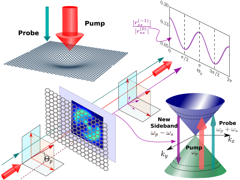
Figure 1: Schematic of graphene illuminated by a CW pump beam (red) of frequency $\omega_{p}$ and a frequency shifted probe beam (green) of frequency $\omega_{p}+\omega_{s}$. The third harmonic related non-linear inter-band polarization combines with optical Bloch oscillations to generate a new side-beam (purple) at frequencies $\omega_{p}-\omega_{s}$. The color plot in the center shows the momentum resolved photo-excited population inversion corresponding to the pump beam: $n_{\boldsymbol{k}}^{(0)}=\rho_{cc}^{(0)}-\rho_{vv}^{(0)}$. The new sideband can be detected in the backward propagating beam via the optical intensity and polarization angle dependence of the reflectivity and polarization angle of the sideband.

Here we propose an alternate technique that uses frequency shifted continuous wavefront (CW) optical fields, probing optical non-linearity in the ‘steady state’. In particular we focus on the non-linear optical sideband generation in graphene due to inter-band polarization combined with optical Bloch oscillations Boyd (2008); Schubert et al. (2014). In presence of a CW pump (frequency $\omega_{p}$) and a frequency shifted probe beam ($\omega_{p}+\omega_{s}$) the optically pumped population inversion and the inter-band coherence oscillate at the modulation frequency. Such coherent ‘slushing’ of the inter-band quasiparticles excitations leads to a new sideband generation at frequencies $\omega_{p}-\omega_{s}=2\omega_{p}-(\omega_{p}+\omega_{s})$, as shown in Fig. 1. This results in distinct signatures in reflectivity along with non-linear polarization rotation at the new sideband frequency. Our formulation based on the dynamics of density matrix for a generic two band systems, can be easily applied to other materials as well.

The predicted sideband generation is a direct consequence of non-degenerate four-wave mixing due to third-order non-linearity in graphene Boyd (2008); Zhang and Voss (2011). Estimation of the corresponding intensity threshold and polarization rotation offers an alternative technique for probing non-linear optical effects and relaxation rates with CW fields in graphene Zhang and Voss (2011). Furthermore, the formulation is applicable from THz to optical domain with applications including switching with controlled non-linear phase shifts approaching $\pi/2$ with reasonable incident CW power and cascaded generation of frequency combs Burghoff et al. (2014).

II Two band model

Our formulation starts with Hamiltonian of an electronic system interacting with an electro-magnetic field. It can be described using the dipole approximation Aversa and Sipe (1995), i.e., $\hat{H}=\hat{H}_{0}+e{\bf E}\cdot{\hat{\bf r}}$. Here $\hat{H}_{0}$ is the bare Hamiltonian, $e$ is the electronic charge, and ${\bf E}$ is the electric field. For simplicity we focus on a generic two band system Singh et al. (2017, 2018a, 2018b), with its quasiparticle dispersion described by the Hamiltonian, $\hat{H}_{0}=\sum_{\boldsymbol{k}}{\bf h}_{\boldsymbol{k}}\cdot\boldsymbol{\sigma}$, where ${\bf h}_{\boldsymbol{k}}=(h_{0{\boldsymbol{k}}},h_{1{\boldsymbol{k}}},h_{2{\boldsymbol{k}}},h_{3{\boldsymbol{k}}})$ is a vector composed of real scalar elements and $\boldsymbol{\sigma}=(\openone_{2},\sigma_{x},\sigma_{y},\sigma_{z})$ is a vector composed of the $2\times 2$ identity and the three Pauli matrices. The eigenvalues for conduction/valence band are, $\varepsilon^{c/v}_{\boldsymbol{k}}=h_{0{\boldsymbol{k}}}\pm g_{\boldsymbol{k}}$, where $g_{\boldsymbol{k}}\equiv\sqrt{h_{1{\boldsymbol{k}}}^{2}+h_{2{\boldsymbol{k}}}^{2}+h_{3{\boldsymbol{k}}}^{2}}$. Accordingly, the state vectors are given by, $\hat{H}_{0}|\psi^{c/v}_{\boldsymbol{k}}\rangle=\varepsilon^{c/v}_{\boldsymbol{k}}|\psi^{c/v}_{\boldsymbol{k}}\rangle$. The frequency shifted electromagnetic field is, ${\bf E}(t)={\rm Re}\left[{\bf E}_{p}e^{-i\omega_{p}t}+{\bf E}_{s}e^{-i(\omega_{p}+\omega_{s})t}\right],$ composed of a primary pump beam (of amplitude $|{\bf E}_{p}|$ and frequency $\omega_{p}$) and a probe beam (of amplitude $|{\bf E}_{s}|\ll|{\bf E}_{p}|$ and frequency $\omega_{p}+\omega_{s}$, where $\omega_{s}\ll\omega_{p}$). In general the pump and the probe fields can have different polarization angles, $\Theta_{p}$ and $\Theta_{s}$, respectively, so that ${\bf E}_{p}=|{\bf E}_{p}|\left(\cos\Theta_{p},\sin\Theta_{p}\right)$ and ${\bf E}_{s}=|{\bf E}_{s}|\left(\cos\Theta_{s},\sin\Theta_{s}\right)$ for vertical incidence.

The dynamics of the two band system described above is obtained by analytically solving the equation of motion (EOM) for the density matrix ($\rho^{ij}_{\boldsymbol{k}}$). The diagonal elements of $\rho_{\boldsymbol{k}}^{ij}$ comprise of the carrier distribution in the conduction ($\rho^{cc}_{\boldsymbol{k}}$) and valence ($\rho^{vv}_{\boldsymbol{k}}$) bands, while the off-diagonal elements $\rho^{vc}_{\boldsymbol{k}}=(\rho^{cv}_{\boldsymbol{k}})^{*}\equiv p_{\boldsymbol{k}}$ capture the inter-band coherence. The incident optical field ‘pumps’ the carriers from the valence band to the conduction band via vertical transitions. This optical pumping of carriers is countered by damping terms originating from the vacuum fluctuations, electron-electron interactions, electron-phonon interactions, and disorder, leading to a finite population inversion ($n_{\boldsymbol{k}}=\rho^{cc}_{\boldsymbol{k}}-\rho^{vv}_{\boldsymbol{k}}$) – shown in Fig. 1. Including the damping terms phenomenologically in the EOM of the density matrix leads to the following set of coupled optical Bloch equation (OBE) Chaves et al. (2016); Singh et al. (2017, 2018a, 2018b),

$$\partial_{t}n_{\boldsymbol{k}} = 4~{}{\rm Im}\left[{\Omega}^{cv}_{\boldsymbol{k}}p_{\boldsymbol{k}}\right]-\gamma_{1}\left(n_{\boldsymbol{k}}-n^{\rm eq}_{\boldsymbol{k}}\right),$$ (1)

$$\partial_{t}p_{\boldsymbol{k}} = i\omega_{\boldsymbol{k}}p_{\boldsymbol{k}}-i{\Omega}^{vc}_{\boldsymbol{k}}n_{\boldsymbol{k}}-\gamma_{2}p_{\boldsymbol{k}}~{}.$$ (2)

The inter-band Rabi frequency can be expressed in terms of the inter-band optical matrix element ${\bf M}^{vc}_{\boldsymbol{k}}\equiv\langle\psi^{v}_{\boldsymbol{k}}|e\nabla_{\boldsymbol{k}}\hat{H}_{0}/\hbar|\psi^{c}_{\boldsymbol{k}}\rangle$ as: $\hbar{\Omega}^{vc}_{\boldsymbol{k}}(t)=i{\bf E}(t)\cdot{\bf M}^{vc}_{\boldsymbol{k}}/\omega_{\boldsymbol{k}}$, where $\omega_{\boldsymbol{k}}=(\varepsilon^{c}_{\boldsymbol{k}}-\varepsilon^{v}_{\boldsymbol{k}})/\hbar$ is the vertical transition frequency . In Eqs. (1)-(16), $\gamma_{1}$ and $\gamma_{2}$ are the phenomenological damping rates of the inter-band population inversion and coherence, respectively. For simplicity, we assume these rates to be constants. Note that this ‘constant damping rate’ approximation allows us to proceed analytically, and it still captures all the relevant physics qualitatively. A more involved modelling of the damping constants, as done in Ref. [Semnani et al., 2018], also yields a very similar results for the population inversion and the interband coherence.

III Steady state solution

For incident CW field, competition between optical pumping and decay rates, results in an eventual steady state. In this regime, analytical solutions can be obtained by making the following ansatz for the population inversion and inter-band coherence Boyd (2008):

$$n_{\boldsymbol{k}} = n_{\boldsymbol{k}}^{(0)}+n_{\boldsymbol{k}}^{(1)}e^{-i\omega_{s}t}+n_{\boldsymbol{k}}^{(-1)}e^{i\omega_{s}t}~{},$$ (3)

$$p_{\boldsymbol{k}} = \left[p_{\boldsymbol{k}}^{(0)}+p_{\boldsymbol{k}}^{(1)}e^{-i\omega_{s}t}+p_{\boldsymbol{k}}^{(-1)}e^{i\omega_{s}t}\right]e^{i\omega_{p}t}~{}.$$ (4)

Here, the superscript $(0)$ is used to denote the steady state solution of the OBEs in presence of CW pump field leading to optical response at frequency $\omega_{p}$ Chaves et al. (2016); Singh et al. (2017, 2018a, 2018b). Presence of a probe field leads to slowly oscillating side-bands. Significant among these are the response (defined in terms of optical conductivities) at frequencies $\omega_{p}\pm\omega_{s}$, denoted by superscript (1) and (-1) in Eq. (11) and Eq. (12) below. The side-band at $\omega_{p}-\omega_{s}$ is generated as a result of interaction between two photons of pump field with one photon of the probe field [$\omega_{p}-\omega_{s}=2\omega_{p}-(\omega_{p}+\omega_{s})$]. The ansatz in Eqs. (3)-(4) for the population inversion and inter-band coherence quantifies this. The addition of $n^{(-1)}_{\boldsymbol{k}}(=[n^{(1)}_{\boldsymbol{k}}]^{*})$, is mandated to make the population inversion real. This in turn forces the terms added in Eq. (4) for the coherence which highlights the systems response at frequencies $\omega_{p}\pm\omega_{s}$.

Using the ansatz of Eq. (3) in Eqs. (1)-(16), and taking long time average for the steady state, we obtain

$$\frac{n^{(0)}_{\boldsymbol{k}}}{n^{\rm eq}_{\boldsymbol{k}}}=\left(1+\zeta^{2}\gamma_{2}^{2}\frac{\omega^{2}}{\omega_{\boldsymbol{k}}^{2}}~{}\frac{|{\bf e}_{p}\cdot\tilde{\bf M}^{cv}_{\boldsymbol{k}}|^{2}}{(\omega_{\boldsymbol{k}}-\omega_{p})^{2}+\gamma_{2}^{2}}\right)^{-1}.$$ (5)

Here, ${\bf e}_{p}={\bf E}_{p}/|{\bf E}_{p}|$, $\tilde{\bf M}^{cv}_{\boldsymbol{k}}={\bf M}^{cv}_{\boldsymbol{k}}/{ev_{F}}$ and we have defined the dimensionless parameter $\zeta=e|{\bf E}_{p}|v_{F}/(\hbar\omega\sqrt{\gamma_{1}\gamma_{2}})$ - which uniquely characterizes the non-linearity in the system Chaves et al. (2016); Singh et al. (2017, 2018a, 2018b). See Appendix for the details of the questions. Equation (5) can be systematically expanded in powers of $\zeta$ with $\zeta\to 0$ denoting the equilibrium distribution (Fermi function denoted by $n^{\rm eq}_{\boldsymbol{k}}$) in absence of optical interactions, while the $\zeta^{2}$ terms denote the $|{\bf E}_{p}|^{2}$ correction to the modified distribution function. The $\zeta\to\infty$ limit is the saturation limit of maximum population inversion with $n^{(0)}_{{\boldsymbol{k}}}\to 0$. The sideband population inversion corresponding to the probe frequency component $(\omega_{p}+\omega_{s})$ Note (1) can be expressed as,

$$n^{(1)}_{\boldsymbol{k}}=n^{(0)}_{\boldsymbol{k}}\left({\bf E}_{s}\cdot{\bf M}^{cv}_{\boldsymbol{k}}\right)\left({\bf E}^{*}_{p}\cdot{\bf M}^{vc}_{\boldsymbol{k}}\right)\xi_{\boldsymbol{k}}~{}.$$ (6)

Here, we have defined,

$$\xi_{\boldsymbol{k}}=\frac{\mathcal{P}_{\boldsymbol{k}}}{2\hbar^{2}\omega^{2}_{\boldsymbol{k}}(\omega_{s}+i\gamma_{1})+|{\bf E}_{p}\cdot{\bf M}^{cv}_{\boldsymbol{k}}|^{2}~{}\mathcal{Q}_{\boldsymbol{k}}}~{}$$ (7)

$$\mathcal{P}_{\boldsymbol{k}}=\frac{-(\omega_{s}+2i\gamma_{2})}{\left[\omega_{\boldsymbol{k}}-\omega_{p}+i\gamma_{2}\right]\left[\omega_{\boldsymbol{k}}-(\omega_{p}+\omega_{s})-i\gamma_{2}\right]}~{},$$ (8)

$$\mathcal{Q}_{\boldsymbol{k}}=\frac{2~{}(\omega_{s}+i\gamma_{2})}{\left[\omega_{\boldsymbol{k}}-(\omega_{p}+\omega_{s})-i\gamma_{2}\right]\left[\omega_{\boldsymbol{k}}-(\omega_{p}-\omega_{s})+i\gamma_{2}\right]}.$$

It can easily be checked that $|n^{(1)}_{{\boldsymbol{k}}}|\to 0$ in both the limiting cases of vanishing intensity of the pump beam ($\zeta\to 0$) as well as in the saturation limit ($\zeta\to\infty$), as expected. Recall that $n_{\boldsymbol{k}}^{(-1)}=[n_{\boldsymbol{k}}^{(1)}]^{*}$ and the analytical expressions for the components of the inter-band coherence are presented in Appendix A. These $\omega_{-1}$ sideband components of the density matrix generate a new optical sideband whose amplitude and polarization depend on the amplitude and polarization of the incident pump beam.

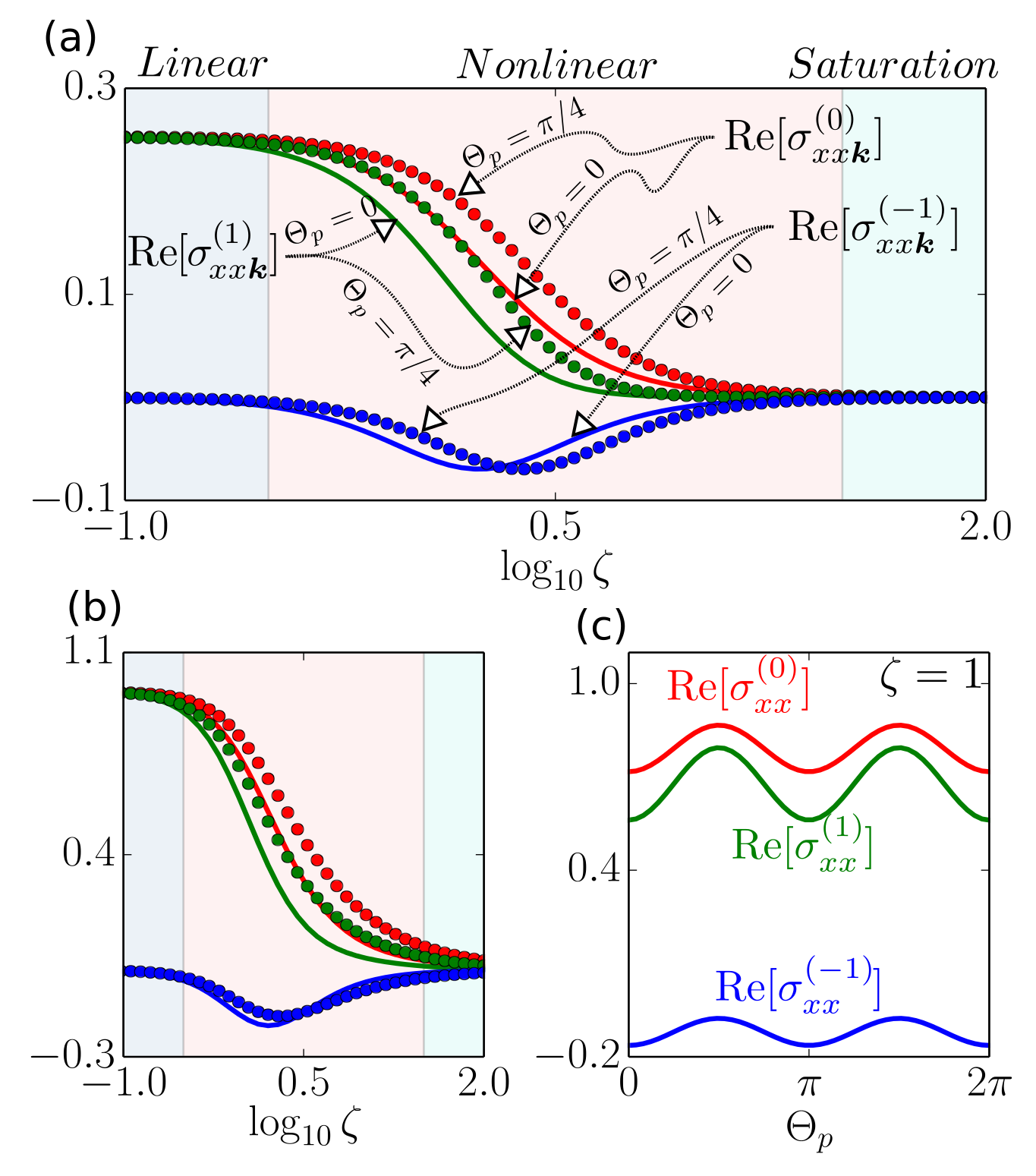
Figure 2: (a) Real part of the momentum resolved conductivity kernel corresponding to the pump ($\sigma^{(0)}_{xx\boldsymbol{k}}$ - in red), probe ($\sigma^{(1)}_{xx\boldsymbol{k}}$ - in green) and the newly generated sideband ($\sigma^{(-1)}_{xx\boldsymbol{k}}$ - in blue) as a function of $\log_{10}\zeta$ for $\Theta_{p}=0$ (solid curve) and $\Theta_{p}=\pi/4$ (dotted curve). Here $\omega_{\boldsymbol{k}}=0.8\omega_{p}$ and $\hat{\boldsymbol{k}}=(0,1)$. (b) The corresponding integrated optical conductivities (in units of $\sigma_{0}=e^{2}/{4\hbar})$ as a function of $\log_{10}\zeta$. As expected, both $\sigma^{(0)}_{xx}$ and $\sigma^{(1)}_{xx}$ display linear response behaviour ($\to\sigma_{0}$) as $\zeta\to 0$. However, the newly generated $\sigma^{(-1)}_{xx}$ is finite only after the onset of the nonlinear response regime ($\zeta\approx 1$). (c) The polarization angle dependence of longitudinal conductivities for $\zeta=1$. Other parameters are: $\omega_{p}=5\times 10^{14}s^{-1}$, $\gamma_{1}=1\times 10^{12}s^{-1}$, $\gamma_{2}=5\times 10^{13}s^{-1}$ and $\mu=0$.

IV Optical conductivity

The optical conductivity at different frequencies can now be obtained via the calculation of the charge current response in the frequency domain: ${\bf J}=\sum_{\boldsymbol{k}}{\rm Trace}(\rho_{\boldsymbol{k}}{\bf M}_{\boldsymbol{k}})=\sigma^{(0)}E_{p}+\sigma^{(1)}E_{s}+\sigma^{(-1)}E_{s}$, where ${\bf M}_{\boldsymbol{k}}/e$ is the effective velocity operator. Here $\sigma^{(0)}$ and $\sigma^{(\pm 1)}$ are non-linear functions of $E_{p}$, capturing the response at frequencies $\omega_{p}$ and $\omega_{p}\pm\omega_{s}$, respectively. The corresponding optical conductivity matrix can be expressed as a Brillouin zone sum of the momentum resolved conductivity matrix: ${\boldsymbol{\sigma}}^{(i)}=(2\pi)^{-d}\int_{\rm BZ}{d\boldsymbol{k}}~{}\sigma^{(i)}_{\boldsymbol{k}}$, with $i=0,\pm 1$ and $d$ denoting the dimensionality of the system. The momentum resolved optical conductivity matrix corresponding to the pump frequency $\omega_{p}$ is given by

$${\boldsymbol{\sigma}}^{(0)}_{{\boldsymbol{k}}}=\frac{in^{(0)}_{{\boldsymbol{k}}}}{\hbar\omega_{\boldsymbol{k}}}\frac{{\bf M}^{vc}_{\boldsymbol{k}}{\otimes}{\bf M}^{cv}_{\boldsymbol{k}}}{\omega_{\boldsymbol{k}}-\omega^{\prime}_{p}}.$$ (10)

Here, $\omega_{p}^{\prime}\equiv\omega_{p}+i\gamma_{2}$ and ${\otimes}$ denotes the outer product of the optical matrix element vectors. The momentum resolved optical conductivity corresponding to the probe frequency $(\omega_{p}+\omega_{s})$ sideband is

$${\boldsymbol{\sigma}}^{(1)}_{{\boldsymbol{k}}}={\boldsymbol{\sigma}}^{(0)}_{{\boldsymbol{k}}}\frac{1+|{\bf E}_{p}\cdot{\bf M}^{cv}_{\boldsymbol{k}}|^{2}\xi_{\bf k}}{[\omega_{\boldsymbol{k}}-(\omega_{p}+\omega_{s})^{{}^{\prime}}][\omega_{\boldsymbol{k}}-\omega^{\prime}_{p}]^{-1}}~{}.$$ (11)

Equation (11) clearly emphasizes the gain in the optical response at the probe frequency $\omega_{p}+\omega_{s}$. As stated earlier, the response at frequencies $\omega_{p}$ and $(\omega_{p}+\omega_{s})$ interfere leading to a sideband generation at the frequency $\omega_{-1}=\omega_{p}-\omega_{s}$. The details of the calculations are presented in Appendix A and B.

The momentum resolved optical conductivity due to the newly generated sideband is given by,

$${\boldsymbol{\sigma}}^{(-1)}_{{\boldsymbol{k}}}={\boldsymbol{\sigma}}^{(0)}_{{\boldsymbol{k}}}\frac{\left({\bf M}^{vc}_{\boldsymbol{k}}{\otimes}{\bf M}^{cv}_{\boldsymbol{k}}\right)^{-1}\left({\bf M}^{vc}_{\boldsymbol{k}}{\otimes}{\bf M}^{vc}_{\boldsymbol{k}}\right)\left({\bf E}_{p}\cdot{\bf M}^{cv}_{\boldsymbol{k}}\right)^{2}\xi^{*}_{\bf k}}{[\omega_{\boldsymbol{k}}-(\omega_{p}-\omega_{s})^{{}^{\prime}}][\omega_{\boldsymbol{k}}-\omega^{\prime}_{p}]^{-1}}~{}.$$ (12)

Equation (12) highlights the optical response generated at the new sideband frequency $\omega_{p}-\omega_{s}$, and is one of the significant finding of this work. This new sideband response originates from the third order non-linearity in graphene. The dependence of the longitudinal optical conductivities on the non-linearity parameter $\zeta\propto|{\bf E}_{p}|$ and the pump polarization angle $\Theta_{p}$ is shown in Fig. 2. The transverse component of the optical conductivity are presented in Fig. 7. As expected, both $\sigma_{xx}^{(0)}$ and $\sigma_{xx}^{(1)}$ reduce to the universal optical conductivity of graphene, $\sigma_{0}=e^{2}/(4\hbar)$, in the linear response regime of $\zeta\to 0$. However, the new sideband contribution $\sigma_{xx}^{(-1)}$ is finite only in the non-linear regime of $\zeta\approx 1$, and vanishes in the linear response as well as in the saturation regime ($\zeta\gg 1$).

Table 1: The reflection coefficients in two dimensional materials in terms of optical conductivities Yoshino (2013); Singh et al. (2018b). Here we have defined, ${\tilde{\sigma}}_{ij}={\sigma}_{ij}/\sigma_{0}$, $\sigma_{0}=e^{2}/(4\hbar)$, and $\tilde{Z}=2/(\pi\alpha_{F}\tilde{\sigma}_{d})$ where $\alpha_{F}\approx 1/137$ is the fine structure constant, and $\tilde{\sigma}_{d}=\left(2/{\pi\alpha_{F}}+{\tilde{\sigma}}_{xx}\right)\left(2/{\pi\alpha_{F}}+{\tilde{\sigma}}_{yy}\right)-{\tilde{\sigma}}_{xy}^{2}$ Note (2).

Coefficient	Exact expression	${\cal O}(\alpha_{F})$
$r_{ss}$	$\tilde{Z}\left(\tilde{Z}\tilde{\sigma}_{d}+{\tilde{\sigma}}_{yy}\right)-1$	$-{\tilde{\sigma}}_{xx}/(\tilde{Z}\tilde{\sigma}_{d})$
$r_{pp}$	$1-\tilde{Z}\left(\tilde{Z}\tilde{\sigma}_{d}+\tilde{\sigma}_{xx}\right)$	${\tilde{\sigma}}_{yy}/(\tilde{Z}\tilde{\sigma}_{d})$
$r_{sp}$	$-\tilde{Z}{\tilde{\sigma}}_{xy}$	$-{\tilde{\sigma}}_{xy}/(\tilde{Z}\tilde{\sigma}_{d})$
$\chi_{s\rm Kerr}$	$-r_{ps}/r_{ss}$	${\sigma}_{xy}/{\sigma}_{xx}$
$\chi_{p\rm Kerr}$	$r_{sp}/r_{pp}$	$-{\sigma}_{xy}/{\sigma}_{yy}$

V Experimental implications of the new sideband

The generated sideband would leave its signature in a range of optical and photo-conductivity measurements Prechtel et al. (2012). Here, we focus on its impact in optical reflectivity, In particular, we explore the pump power and polarization angle dependence of the reflectivity (amplitude and phase in $r=\sqrt{\cal R}e^{i\Phi}$), and the Kerr angle $\Theta_{\rm Kerr}$ Yoshino (2013); Singh et al. (2018b). For graphene, though small, the reflectivity is routinely measured Nair et al. (2008); Mak et al. (2008); Singh et al. (2017, 2018b), while the phase of the reflection coefficient can be measured using a generic interference setup. Thus ${\cal R}$, $\Phi$ and $\Theta_{\rm Kerr}$ can be probed as a function of the probe laser power and polarization angle (see Fig. 1). The dependence of the $s$ and $p$ components of the reflection coefficients on the respective optical conductivities in graphene are tabulated in Table 1 .

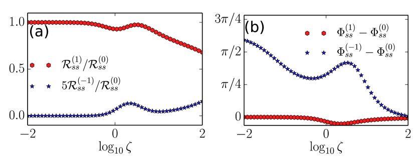
Figure 3: Variation of (a) reflection probability (b) and its phase as a function of the pump field strength ($\log_{10}\zeta$), for the probe, and $\omega_{-1}$ frequencies. The nonlinear $\omega_{-1}$ sideband can also be probed via the interference experiments sensitive to the phase of the reflection coefficient. We have chosen $\Theta_{p}=\pi/4$ for both panels, and other parameters are identical to those of Fig. 2.

To compare the reflection amplitude and phase of the sideband with that of the pump beam, we define the following:

$$\frac{\mathcal{R}^{(\lambda)}_{ss}}{\mathcal{R}^{(0)}_{ss}}=\frac{|r^{(\lambda)}_{ss}|^{2}}{|r^{(0)}_{ss}|^{2}}~{},~{}~{}~{}~{}\tan\Phi^{(\lambda)}=\frac{{\rm Im}[r^{(\lambda)}_{ss}]}{{\rm Re}[r^{(\lambda)}_{ss}]}~{},$$ (13)

where $\lambda=\pm 1$ for reflectance measured at the sideband frequencies $\omega_{p}\pm\omega_{s}$. The dependence of the ratios of the reflectance and $\Phi$ defined in Eq. 13, is shown in Fig. 3 as a function of the pump beam intensity ($\propto\zeta^{2}$). Clearly the $\omega_{-1}$ sideband response at manifests only in the non-linear regime of $\zeta\approx 1$. In the optical regime (say $\omega_{p}=5\times 10^{14}{\rm s^{-1}}$), the estimated damping constants in graphene Zhang and Voss (2011) are $\gamma_{1}\approx 10^{12}{\rm s^{-1}},\gamma_{2}\approx 5\times 10^{13}{\rm s^{-1}}$. Using these values, the $\zeta\approx 1$ condition in graphene corresponds to a CW laser intensity $\approx 10^{5}~{}{\rm Wcm^{-2}}$, which is reasonable Prechtel et al. (2012). Furthermore, at reasonable CW powers we also observe non-linear phase shifts in excess of $\pi/2$ for the new sideband. Such large non-linear phase shifts is of great interest in a range of switching applications in THz and optical domains. The polarization angle $\Theta_{p}$ dependence of the reflection probability and its phase is shown in Fig. 4(a)-(b).

Non-linear optical response in graphene also generates a finite $\sigma_{xy}$, which in turn leads to Kerr rotation (polarization rotation of the reflected beam)Yoshino (2013); Singh et al. (2018b). The Kerr rotation angle for $s-$ and $p-$ polarized incident pump beam is given by Yoshino (2013); Singh et al. (2018b),

$$\Theta^{(\lambda)}_{s/p{\rm Kerr}}=\frac{1}{2}\tan^{-1}\left(\frac{2{{\rm Re}[\chi^{(\lambda)}_{s/p{\rm Kerr}}]}}{1-|\chi^{(\lambda)}_{s/p{\rm Kerr}}|^{2}}\right)~{},$$ (14)

where $\chi_{s/p{\rm Kerr}}$ can be expressed in terms of the reflection coefficients (see Table 1). The variation of the Kerr angle for the $s$ and $p$ components for pump, probe and the new sideband beam as a function of $\Theta_{p}$ is shown in Fig. 4 (c)-(d). The polarization rotation of the $\omega_{-1}$ sideband seems to be significantly large and different from that corresponding to the pump and probe frequencies.

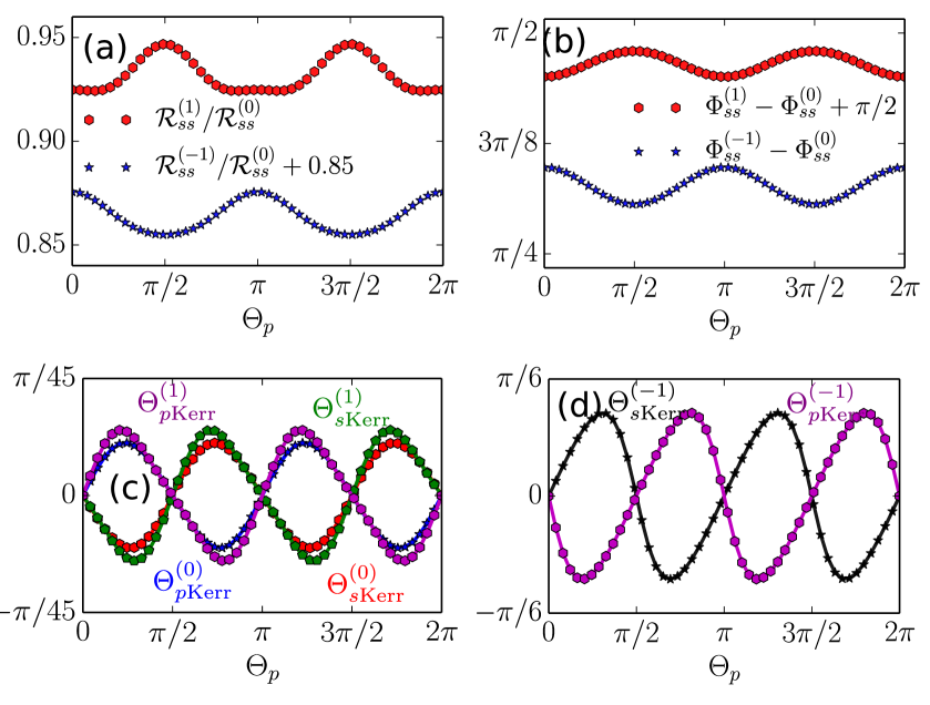
Figure 4: Dependence of (a) the probability and (b) the phase of the reflection coefficient for the probe and $\omega_{-1}$ sideband as a function of $\Theta_{p}$. The polarization rotation of the reflected beam (Kerr angle) for $s-$ and $p-$ polarized beams as a function of $\Theta_{p}$ are shown in c) for the pump and probe frequencies and in d) for the $\omega_{-1}$ frequency. Here $\zeta=1$ and other parameters are identical to those of Fig. 2.

VI Summary

In summary, we predict generation of a new modulated optical sideband in graphene in presence of a CW frequency shifted pump-probe setup. Physically, the ‘slushing’ of the inter-band coherence due to interference of the pump and the probe results in the generated sideband that carries unique signature of the third order non-linear response in graphene. Experimentally, this manifests in the polarization, reflectivity, and in the phase of the reflection coefficient (see Fig. 3) at the sideband frequencies. In particular, the peak of the sideband gain occurs at a thereshold, characterized by a single parameter $\zeta$ set by system decay rates and the pump power. A careful characterization of generated sideband gain can thereby provide a direct method of characterizing non-linear response of two-band systems with CW fields, in contrast to traditional, technologically involved time domain measurements. It also suggests a range of applications that include switching of frequency sidebands using non-linear phase shifts and generation of frequency combs.

Appendix A Steady state density matrix in presence of pump and probe fields

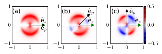
Figure 5: Real part of population inversion corresponding to probe frequency ($\Re[n_{\bf k}^{(1)}]$) for, (a) $\hat{\bf e}_{p}=\hat{\boldsymbol{x}}$, $\hat{\bf e}_{s}=\hat{\boldsymbol{x}}$, (b) $\hat{\bf e}_{p}=(\hat{\boldsymbol{x}}+\hat{\boldsymbol{y}})/\sqrt{2}$, $\hat{\bf e}_{s}=\hat{\boldsymbol{x}}$ and (c) $\hat{\bf e}_{p}=\hat{\boldsymbol{y}}$, $\hat{\bf e}_{s}=\hat{\boldsymbol{x}}$. Other parameters are: $\omega_{p}=5\times 10^{14}s^{-1}$, $\gamma_{1}=1\times 10^{12}s^{-1}$, $\gamma_{2}=5\times 10^{13}s^{-1}$ and the chemical potential $\mu=0$.

In this section we obtain analytical results for the steady state density matrix as a solution of the optical Bloch equations (OBEs) in the presence of a pump as well as a probe field. The OBEs, including phenomenological damping terms are given by Chaves et al. (2016); Singh et al. (2017, 2018a, 2018b),

$$\partial_{t}n_{\boldsymbol{k}} = 4~{}{\rm Im}\left[{\Omega}^{cv}_{\boldsymbol{k}}p_{\boldsymbol{k}}\right]-\gamma_{1}\left(n_{\boldsymbol{k}}-n^{\rm eq}_{\boldsymbol{k}}\right),$$ (15)

$$\partial_{t}p_{\boldsymbol{k}} = i\omega_{\boldsymbol{k}}p_{\boldsymbol{k}}-i{\Omega}^{vc}_{\boldsymbol{k}}n_{\boldsymbol{k}}-\gamma_{2}p_{\boldsymbol{k}}~{}.$$ (16)

The ansatz for the solution of population inversion, $n_{\boldsymbol{k}}$ and the inter-band coherence $p_{\boldsymbol{k}}$ is motivated by the fact that the relatively weak probe field has only perturbative impact on the steady state population inversion achieved under the action of the pump field alone. Following BoydBoyd (2008), we can express $n_{\boldsymbol{k}}$ and $p_{\boldsymbol{k}}$ as,

$$n_{\boldsymbol{k}} = n^{(0)}_{\boldsymbol{k}}+n^{(1)}_{\boldsymbol{k}}e^{-i\omega_{s}t}+n^{(-1)}_{\boldsymbol{k}}e^{i\omega_{s}t}~{},$$ (17)

$$p_{\boldsymbol{k}} = \left(p^{(0)}_{\boldsymbol{k}}+p^{(1)}_{\boldsymbol{k}}e^{-i\omega_{s}t}+p^{(-1)}_{\boldsymbol{k}}e^{i\omega_{s}t}\right)e^{i\omega_{p}t}~{},$$

where $n^{(0)}_{\boldsymbol{k}},n^{(1)}_{\boldsymbol{k}}$ and $n^{(-1)}_{\boldsymbol{k}}$ are time independent in the steady state. Here we assume that $\omega_{s}\ll\omega_{p}$ and we ignore the second order terms like $n^{(1)}p^{(1)}_{\boldsymbol{k}},n^{(1)}p^{(-1)}_{\boldsymbol{k}}$ and so on. Since the total population inversion $n_{\boldsymbol{k}}$ has to be a real physical quantity, we have $({n^{(1)}_{\boldsymbol{k}}})^{*}=n^{(-1)}_{\boldsymbol{k}}$.

The time derivative of the population inversion and the inter-band polarization are given by,

$$\dot{n}_{\boldsymbol{k}} = -i\omega_{s}~{}n^{(1)}_{\boldsymbol{k}}e^{-i\omega_{s}t}+i\omega_{s}~{}n^{(-1)}_{\boldsymbol{k}}e^{i\omega_{s}t}~{},$$ (18)

$$\dot{p}_{\boldsymbol{k}} = i\omega_{p}~{}p^{(0)}_{\boldsymbol{k}}e^{i\omega_{p}t}+i(\omega_{p}-\omega_{s})~{}p^{(1)}_{\boldsymbol{k}}e^{i(\omega_{p}-\omega_{s})t}$$ (19)

$$+ i(\omega_{p}+\omega_{s})~{}p^{(-1)}_{\boldsymbol{k}}e^{i(\omega_{p}+\omega_{s})t}~{}.$$

Using the expression for $\Omega^{vc}_{\boldsymbol{k}}$ and the full form of the applied pump and probe electric field, a straightforward calculation yields,

$$-i\Omega^{vc}_{\boldsymbol{k}}{n}_{\boldsymbol{k}} = \Bigg{[}\frac{{\bf E}_{p}\cdot{\bf M}^{vc}_{\boldsymbol{k}}}{{2\hbar\omega_{\boldsymbol{k}}}}n^{(0)}_{\boldsymbol{k}}e^{-i\omega_{p}t}+\frac{{\bf E}^{*}_{p}\cdot{\bf M}^{vc}_{\boldsymbol{k}}}{{2\hbar\omega_{\boldsymbol{k}}}}n^{(0)}_{\boldsymbol{k}}e^{i\omega_{p}t}$$ (20)

$$+ \Big{(}\frac{{\bf E}_{p}\cdot{\bf M}^{vc}_{\boldsymbol{k}}}{{2\hbar\omega_{\boldsymbol{k}}}}n^{(1)}_{\boldsymbol{k}}+\frac{{\bf E}_{s}\cdot{\bf M}^{vc}_{\boldsymbol{k}}}{{2\hbar\omega_{\boldsymbol{k}}}}n^{(0)}_{\boldsymbol{k}}\Big{)}e^{-i(\omega_{p}+\omega_{s})t}$$

$$+ \Big{(}\frac{{\bf E}^{*}_{s}\cdot{\bf M}^{vc}_{\boldsymbol{k}}}{{2\hbar\omega_{\boldsymbol{k}}}}n^{(0)}_{\boldsymbol{k}}+\frac{{\bf E}^{*}_{p}\cdot{\bf M}^{vc}_{\boldsymbol{k}}}{{2\hbar\omega_{\boldsymbol{k}}}}n^{(-1)}_{\boldsymbol{k}}\Big{)}e^{i(\omega_{p}+\omega_{s})t}$$

$$+ \frac{{\bf E}_{p}\cdot{\bf M}^{vc}_{\boldsymbol{k}}}{{2\hbar\omega_{\boldsymbol{k}}}}n^{(-1)}_{\boldsymbol{k}}e^{-i(\omega_{p}-\omega_{s})t}$$

$$+ \frac{{\bf E}^{*}_{p}\cdot{\bf M}^{vc}_{\boldsymbol{k}}}{{2\hbar\omega_{\boldsymbol{k}}}}n^{(1)}_{\boldsymbol{k}}e^{i(\omega_{p}-\omega_{s})t}\Bigg{]}.$$

Ignoring the counter rotating terms in Eq. (20) and using Eq. (19), we obtain

$$p^{(0)}_{\boldsymbol{k}}=\frac{i}{2\hbar\omega_{\boldsymbol{k}}}\left[\frac{n^{(0)}_{\boldsymbol{k}}\left({\bf E}^{*}_{p}\cdot{\bf M}^{vc}_{\boldsymbol{k}}\right)}{\omega_{\boldsymbol{k}}-\omega_{p}+i\gamma_{2}}\right],$$ (21)

$$p^{(1)}_{\boldsymbol{k}}=\frac{i}{2\hbar\omega_{\boldsymbol{k}}}\left[\frac{n^{(1)}_{\boldsymbol{k}}\left({\bf E}^{*}_{p}\cdot{\bf M}^{vc}_{\boldsymbol{k}}\right)}{\omega_{\boldsymbol{k}}-(\omega_{p}-\omega_{s})+i\gamma_{2}}\right],$$ (22)

and,

$$p^{(-1)}_{\boldsymbol{k}}=\frac{i}{2\hbar\omega_{\boldsymbol{k}}}\left[\frac{\left({\bf E}^{*}_{p}\cdot{\bf M}^{vc}_{\boldsymbol{k}}\right)n^{(-1)}_{\boldsymbol{k}}+\left({\bf E}^{*}_{s}\cdot{\bf M}^{vc}_{\boldsymbol{k}}\right)n^{(0)}_{\boldsymbol{k}}}{\omega_{\boldsymbol{k}}-(\omega_{p}+\omega_{s})+i\gamma_{2}}\right].$$ (23)

Note that we have done the calculations keeping the counter-rotating terms as well, and explicitly checked that the results are qualitatively in very good agreement to the ones reproduced here.

Similar to Eq. (20), we have,

$$\Omega^{cv}_{\boldsymbol{k}}p_{\boldsymbol{k}} = -i\frac{{\bf E}_{p}\cdot{\bf M}^{cv}_{\boldsymbol{k}}}{2\hbar\omega_{\boldsymbol{k}}}p^{(0)}_{\boldsymbol{k}}-i\frac{{\bf E}_{p}\cdot{\bf M}^{cv}_{\boldsymbol{k}}}{2\hbar\omega_{\boldsymbol{k}}}p^{(-1)}_{\boldsymbol{k}}e^{i\omega_{s}t}$$

$$- i\left(\frac{{\bf E}_{p}\cdot{\bf M}^{cv}_{\boldsymbol{k}}}{2\hbar\omega_{\boldsymbol{k}}}p^{(1)}_{\boldsymbol{k}}+\frac{{\bf E}_{s}\cdot{\bf M}^{cv}_{\boldsymbol{k}}}{2\hbar\omega_{\boldsymbol{k}}}p^{(0)}_{\boldsymbol{k}}\right)e^{-i\omega_{s}t}~{}.$$

Substituting Eq. (A) in Eq. (15) we obtain,

$$\gamma_{1}\left(n^{(0)}_{\boldsymbol{k}}-n^{\rm eq}_{\boldsymbol{k}}\right)=-\frac{{\bf E}_{p}\cdot{\bf M}^{cv}_{\boldsymbol{k}}}{\hbar\omega_{\boldsymbol{k}}}p^{(0)}_{\boldsymbol{k}}-\frac{{\bf E}^{*}_{p}\cdot{\bf M}^{vc}_{\boldsymbol{k}}}{\hbar\omega_{\boldsymbol{k}}}{p^{(0)}_{\boldsymbol{k}}}^{*}.$$ (25)

Combining this with Eq. (21), we obtain

$$\frac{n^{(0)}_{\boldsymbol{k}}}{n^{\rm eq}_{\boldsymbol{k}}}=\left[1+\frac{\gamma_{2}}{\gamma_{1}}\frac{1}{\hbar^{2}\omega_{\boldsymbol{k}}^{2}}\frac{|{\bf E}_{p}\cdot{\bf M}^{cv}_{\boldsymbol{k}}|^{2}}{(\omega_{\boldsymbol{k}}-\omega_{p})^{2}+\gamma_{2}^{2}}\right]^{-1}.$$ (26)

Similarly, the population inversion corresponding to the probe frequency can be obtained to be

$$(\gamma_{1}-i\omega_{s})n^{(1)}_{\boldsymbol{k}} = -\frac{{\bf E}_{p}\cdot{\bf M}^{cv}_{\boldsymbol{k}}}{\hbar\omega_{\boldsymbol{k}}}p^{(1)}_{\boldsymbol{k}}-\frac{{\bf E}_{s}\cdot{\bf M}^{cv}_{\boldsymbol{k}}}{\hbar\omega_{\boldsymbol{k}}}p^{(0)}_{\boldsymbol{k}}$$ (27)

$$- \frac{{\bf E}^{*}_{p}\cdot{\bf M}^{vc}_{\boldsymbol{k}}}{\hbar\omega_{\boldsymbol{k}}}{p^{(-1)}_{\boldsymbol{k}}}^{*}.$$

Combining this with Eq. (21), Eq. (22) and Eq. (23), leads to

$$n^{(1)}_{\boldsymbol{k}}=n^{(0)}_{\boldsymbol{k}}\left({\bf E}_{s}\cdot{\bf M}^{cv}_{\boldsymbol{k}}\right)\left({\bf E}^{*}_{p}\cdot{\bf M}^{vc}_{\boldsymbol{k}}\right)\xi_{\boldsymbol{k}}~{}.$$ (28)

Here we have defined

$$\xi_{\boldsymbol{k}}=\frac{\mathcal{P}_{\boldsymbol{k}}}{2\hbar^{2}\omega^{2}_{\boldsymbol{k}}(\omega_{s}+i\gamma_{1})+|{\bf E}_{p}\cdot{\bf M}^{cv}_{\boldsymbol{k}}|^{2}~{}\mathcal{Q}_{\boldsymbol{k}}}~{},$$ (29)

$$\mathcal{P}_{\boldsymbol{k}}=\left(\frac{1}{\omega_{\boldsymbol{k}}-\omega_{p}+i\gamma_{2}}-\frac{1}{\omega_{\boldsymbol{k}}-(\omega_{p}+\omega_{s})-i\gamma_{2}}\right),$$ (30)

and

$$\mathcal{Q}_{\boldsymbol{k}}=\left(\frac{1}{\omega_{\boldsymbol{k}}-(\omega_{p}+\omega_{s})-i\gamma_{2}}-\frac{1}{\omega_{\boldsymbol{k}}-(\omega_{p}-\omega_{s})+i\gamma_{2}}\right).$$ (31)

The real part of the obtained $n^{(1)}_{\boldsymbol{k}}$ is shown in Fig. 5, for different orientation of the polarization angles of the pump beam.

Appendix B Pump, probe and the sideband current density

In this section we calculate the inter-band current density corresponding to the pump, probe and the newly generated sideband frequencies. In presence of a frequency modulated CW light beam, a steady state situation is achieved where a quasi stationary population inversion is obtained as shown explicitly in the previous section. During this period, a non-vanishing steady state inter-band current is maintained because of the finite inter-band coherence or polarization. The momentum resolved current density, at any time $t$ can be expressed in terms of microscopic polarization $p_{\boldsymbol{k}}$ and the optical matrix element ${\bf M}^{cv}_{\boldsymbol{k}}$ as,

$${\bf J}_{\boldsymbol{k}}(t)=-2{\rm Re}[p_{\boldsymbol{k}}(t){\bf M}^{cv}_{\boldsymbol{k}}]~{}.$$ (32)

The total current is given as the sum of all the momentum modes over the Brillouin zone (BZ),

$${\bf J}(t)=\frac{g_{s}g_{v}}{4\pi^{2}}\int{\bf J}_{\boldsymbol{k}}(t)d{\boldsymbol{k}},$$ (33)

where $g_{s}$ and $g_{v}$ represents the spin and valley degeneracy respectively. While using a tight-binding model, this summation is restricted to the first Brillouin zone. On using an effective low energy model, the integral limit is fixed to some cut-off value where the integral kernel is almost zero. In the presence of the probe sideband at $\omega_{p}+\omega_{s}$ frequency, we need to make a similar ansatz for the total current as we did for the components of the density matrix. Thus the total current can be expressed as,

$${\bf J}_{\boldsymbol{k}}(t)=\frac{1}{2}\left[{\boldsymbol{J}}_{\boldsymbol{k}}e^{-i\omega_{p}t}+c.c\right],$$ (34)

where ${\boldsymbol{J}}_{\boldsymbol{k}}={\boldsymbol{J}}^{(0)}_{\boldsymbol{k}}+{\boldsymbol{J}}^{(1)}_{\boldsymbol{k}}e^{-i\omega_{s}t}+{\boldsymbol{J}}^{(-1)}_{\boldsymbol{k}}e^{i\omega_{s}t}.$ Note that the different time dependence of these currents will lead to the generation of electromagnetic fields at different optical frequencies: $\omega_{p}$ and $\omega_{p}\pm\omega_{s}$. Once again, matching the coefficient of $e^{0},e^{i\omega_{s}t}$ and $e^{-i\omega_{s}t}$ terms, we obtain ${\boldsymbol{J}}^{(0)}_{\boldsymbol{k}}=-2~{}{p^{(0)}_{\boldsymbol{k}}}^{*}{\bf M}^{vc}_{\boldsymbol{k}},{\boldsymbol{J}}^{(1)}_{\boldsymbol{k}}=-2~{}{p^{(-1)}_{\boldsymbol{k}}}^{*}{\bf M}^{vc}_{\boldsymbol{k}}$ and ${\boldsymbol{J}}^{(0)}_{\boldsymbol{k}}=-2~{}{p^{(1)}_{\boldsymbol{k}}}^{*}{\bf M}^{vc}_{\boldsymbol{k}}$. This implies that,

$${\boldsymbol{J}}^{(0)}_{\boldsymbol{k}}=\frac{in^{(0)}_{\boldsymbol{k}}}{\hbar\omega_{\boldsymbol{k}}}\frac{{\left({\bf E}_{p}\cdot{\bf M}^{cv}_{\boldsymbol{k}}\right){\bf M}^{vc}_{\boldsymbol{k}}}}{\omega_{\boldsymbol{k}}-\omega_{p}-i\gamma_{2}}~{},$$ (35)

$${\boldsymbol{J}}^{(1)}_{\boldsymbol{k}}=\frac{{\left({\bf E}_{s}\cdot{\bf M}^{cv}_{\boldsymbol{k}}\right){\bf M}^{vc}_{\boldsymbol{k}}}}{\hbar\omega_{\boldsymbol{k}}}\left[\frac{in^{(0)}_{\boldsymbol{k}}\left(1+\xi_{\boldsymbol{k}}|{\bf E}_{p}\cdot{\bf M}^{cv}_{\boldsymbol{k}}|^{2}\right)}{\omega_{\boldsymbol{k}}-(\omega_{p}+\omega_{s})-i\gamma_{2}}\right]~{},$$ (36)

and,

$${\boldsymbol{J}}^{(-1)}_{\boldsymbol{k}}=\frac{in^{(0)}_{\boldsymbol{k}}}{\hbar\omega_{\boldsymbol{k}}}\left[\frac{\left({\bf E}^{*}_{s}\cdot{\bf M}^{vc}_{\boldsymbol{k}}\right){\bf M}^{vc}_{\boldsymbol{k}}{\left({\bf E}_{p}\cdot{\bf M}^{cv}_{\boldsymbol{k}}\right)^{2}}\xi^{*}_{\boldsymbol{k}}}{\omega_{\boldsymbol{k}}-(\omega_{p}-\omega_{s})-i\gamma_{2}}\right]~{}.$$ (37)

We consider the optical electric field associated with the pump and probe beams to be real i.e., ${\bf E}_{p}=|{\bf E}_{p}|\left(\cos\Theta_{p},\sin\Theta_{p}\right)$, and ${\bf E}_{s}=|{\bf E}_{s}|\left(\cos\Theta_{s},\sin\Theta_{s}\right)$, where $|{\bf E}_{p}|$ and $|{\bf E}_{s}|$ are the magnitudes and, $\Theta_{p}$ and $\Theta_{s}$ are the polarization direction of the respective beams.

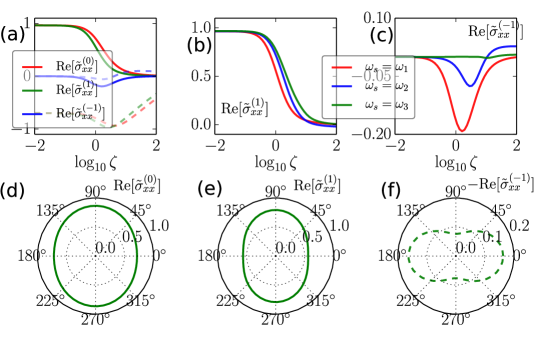
Figure 6: Longitudinal optical conductivities (scaled with $\sigma_{0}=e^{2}/(4\hbar)$) as a function of electric field dependend dimensionless parameter $\zeta$ and polarization. (a) Real (shown in solid) and imaginary part (shown in dashed) corresponding to the pump ($\sigma^{(0)}_{xx}$), probe ($\sigma^{(1)}_{xx}$) and the newly generated sideband ($\sigma^{(-1)}_{xx}$) as a function of $\log_{10}\zeta$ for $\Theta_{p}=0$. (b) and (c) demonstrate the response of $\sigma^{(1)}_{xx}$ and $\sigma^{(-1)}_{xx}$ for three different values of the sideband frequencies, $10^{11}{\rm s^{-1}}$, $5\times 10^{12}{\rm s^{-1}}$ and $5\times 10^{13}{\rm s^{-1}}$, showing that the former increases while the latter decreases with increase in $\omega_{s}$. In (d), (e), and (f) we have shown the dependence of $\sigma^{(0)}_{xx}$, $\sigma^{(1)}_{xx}$ and $\sigma^{(-1)}_{xx}$ w.r.t. $\Theta_{p}$ for $\zeta=1$. Please note that we have shown ${\rm Re}[\sigma^{(-1)}_{xx}]$ in dashed in Fig. 6(f), because of -ve sign, as can also be seen from Fig. 6(c). Other parameters are same as those of Fig. 5.

The Hamiltonian of Graphene in the Fourier space is given as Katsnelson (2012)

$$H=\begin{pmatrix}0&&tf({\boldsymbol{k}})\\ tf^{*}({\boldsymbol{k}})&&0\\ \end{pmatrix}~{},$$ (38)

where the hopping parameter $t$ is roughly equal to $2.7$ eV, $f({\boldsymbol{k}})=e^{i{\boldsymbol{k}}\cdot{\boldsymbol{\delta}_{1}}}+e^{i{\boldsymbol{k}}\cdot{\boldsymbol{\delta}_{2}}}+e^{i{\boldsymbol{k}}\cdot{\boldsymbol{\delta}_{3}}}$,  $\boldsymbol{\delta}_{1}=\frac{a}{2}\left(1,\sqrt{3}\right)$, $\boldsymbol{\delta}_{2}=\frac{a}{2}\left(1,-\sqrt{3}\right)$, $\boldsymbol{\delta}_{3}=a\left(-1,0\right)$, $f^{*}({\boldsymbol{k}})$ is the complex conjugate of $f({\boldsymbol{k}})$ and ${\boldsymbol{k}}=(k_{x},k_{y})$. Thus we have,

$$f({\boldsymbol{k}})=\cos\left[k_{x}a\right]+2\cos\left[{k_{x}a}/{2}\right]\cos\left[{\sqrt{3}k_{y}a}/{2}\right]$$

$$-i\left(\sin\left[k_{x}a\right]-2\sin\left[{k_{x}a}/{2}\right]\cos\left[{\sqrt{3}k_{y}a}/{2}\right]\right).$$ (39)

The energy eigenvalues of Eq. (38) are given by $\varepsilon^{\pm}_{\boldsymbol{k}}=\pm E_{\boldsymbol{k}}$, where $E_{\boldsymbol{k}}=t|f({\boldsymbol{k}})|$. The bandstructure of graphene apparently has 6 Dirac points. However out of these six points, only a pair of Dirac points are not equivalent and are usually referred as ${\bf K}$ and ${\bf K}^{\prime}$ points. Generally these are chosen to be located at

$${\bf K}=\left(\frac{2\pi}{3a},-\frac{2\pi}{3\sqrt{3}a}\right),~{}~{}{\rm and}~{}~{}{\bf K}^{\prime}=\left(\frac{2\pi}{3a},\frac{2\pi}{3\sqrt{3}a}\right)~{}.$$ (40)

The low energy dispersion of graphene close to either of these two Dirac points is given by,

$$H\approx\begin{pmatrix}0&&\hbar v_{F}\left(k_{x}-ik_{y}\right)\\ \hbar v_{F}\left(k_{x}+ik_{y}\right)&&0\\ \end{pmatrix}.$$ (41)

Here, $k$ is measured from either of the Dirac points. For this effective low energy Hamiltonian, the energy eigenvalue is given by $E_{\boldsymbol{k}}=\hbar v_{F}|{\boldsymbol{k}}|$, where the Fermi velocity is known to be $v_{F}=10^{6}{\rm ms^{-1}}$ and $|{\boldsymbol{k}}|=\sqrt{k_{x}^{2}+k_{y}^{2}}$ .

The optical matrix element responsible for the inter-band transition in the generic two band model is Singh et al. (2017),

$${\bf M}_{\boldsymbol{k}}^{vc} = -\frac{e}{\hbar g_{\boldsymbol{k}}h_{\boldsymbol{k}}}\Big{(}-h_{\boldsymbol{k}}^{2}\nabla_{\boldsymbol{k}}h_{3{\boldsymbol{k}}}+(h_{1{\boldsymbol{k}}}h_{3{\boldsymbol{k}}}-ih_{2{\boldsymbol{k}}}g_{{\boldsymbol{k}}})\nabla_{\boldsymbol{k}}h_{1{\boldsymbol{k}}}$$ (42)

$$+ (h_{2{\boldsymbol{k}}}h_{3{\boldsymbol{k}}}+ih_{1{\boldsymbol{k}}}g_{{\boldsymbol{k}}})\nabla_{\boldsymbol{k}}h_{2{\boldsymbol{k}}}~{}\Big{)}.$$

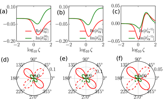
Figure 7: Real and imaginary parts of transverse optical conductivities (scaled with $\sigma_{0}=e^{2}/(4\hbar)$) as a function of electric field dependent dimensionless parameter $\zeta$ and polarization. We have shown (a) Re[$\sigma^{(0)}_{xy}$] and Im[$\sigma^{(0)}_{xy}$], (b) Re[$\sigma^{(1)}_{xy}$] and Im[$\sigma^{(1)}_{xy}$] and (c) Re[$\sigma^{(-1)}_{xy}$] and Im[$\sigma^{(-1)}_{xy}$] as a function of $\log_{10}\zeta$ for $\Theta_{p}=\pi/4$ whereas in (d), (e), and (f) we have shown the same set of variables w.r.t. $\Theta_{p}$ for $\zeta=1$. Please note that the dashed curves represent the negative values of the variables. Other parameters are same as those of Fig. 5.

Specifically for graphene, we have $h_{1{\boldsymbol{k}}}=\hbar v_{F}k_{x}$, $h_{2{\boldsymbol{k}}}=\hbar v_{F}k_{y}$ and $h_{3{\boldsymbol{k}}}=0$. Therefore, the optical matrix element for the low energy Hamiltonian of graphene in Eq. (41) is,

$${\bf M}_{\boldsymbol{k}}^{vc}=iev_{F}\left(\sin\phi_{\boldsymbol{k}},-\cos\phi_{\boldsymbol{k}},0\right),$$ (43)

where the azimuthal angle is given by $\phi_{\boldsymbol{k}}=\tan^{-1}(k_{y}/k_{x})$. Therefore, we have, ${\bf E}_{p}\cdot{\bf M}^{vc}_{\boldsymbol{k}}=-{\bf E}_{p}\cdot{\bf M}^{cv}_{\boldsymbol{k}}=iev_{F}|{\bf E}_{p}|\sin(\phi_{\boldsymbol{k}}-\Theta_{p})$. This leads to

$$\frac{n^{(0)}_{\boldsymbol{k}}}{n^{\rm eq}_{\boldsymbol{k}}}=\left[1+\zeta^{2}\frac{\tilde{\gamma}_{2}^{2}}{\tilde{\omega}^{2}_{\boldsymbol{k}}}\frac{\sin^{2}\left(\phi_{\boldsymbol{k}}-\Theta_{p}\right)}{(\tilde{\omega}_{\boldsymbol{k}}-1)^{2}+\tilde{\gamma}_{2}^{2}}\right]~{}.$$ (44)

where $\zeta=ev_{F}|{\bf E}_{p}|/(\hbar\omega_{p}\sqrt{\gamma_{1}\gamma_{2}})$, $\tilde{\omega}_{\boldsymbol{k}}=\omega_{\boldsymbol{k}}/\omega_{p}$ and $\tilde{\gamma}_{2}=\gamma_{2}/\omega_{p}$. Accordingly we obtain,

$$\sigma^{(0)}_{xx\boldsymbol{k}}=\frac{\sigma_{0}}{\pi^{2}}\frac{in^{(0)}_{\boldsymbol{k}}}{\tilde{\omega}_{\boldsymbol{k}}}\left[\frac{\sin^{2}\phi_{\boldsymbol{k}}}{\tilde{\omega}_{\boldsymbol{k}}-1-i\tilde{\gamma}_{2}}\right],$$ (45)

The total conductivity is obtained by summing the momentum resolved conductivity over the BZ,

$$\sigma^{(0)}_{xx}=\int\tilde{\omega}_{\boldsymbol{k}}d\tilde{\omega}_{\boldsymbol{k}}d\phi_{\boldsymbol{k}}\sigma^{(0)}_{xx\boldsymbol{k}}~{}.$$ (46)

Similarly we obtain,

$$\sigma^{(1)}_{xx\boldsymbol{k}}=\frac{\sigma_{0}}{\pi^{2}}\frac{in^{(0)}_{\boldsymbol{k}}}{\tilde{\omega}_{\boldsymbol{k}}}\left[\frac{\sin^{2}\phi_{\boldsymbol{k}}\left(1+\tilde{\xi}_{\bf k}\sin^{2}\left(\phi_{\boldsymbol{k}}-\Theta_{p}\right)\right)}{\tilde{\omega}_{\boldsymbol{k}}-(1+\tilde{\omega}_{1})-i\tilde{\gamma}_{2}}\right].$$ (47)

Here, we have defined

$$\tilde{\xi}_{\bf k}=\frac{\zeta^{2}\tilde{\gamma_{1}}\tilde{\gamma_{2}}\tilde{\mathcal{P}}_{\boldsymbol{k}}}{2\tilde{\omega}^{2}_{\boldsymbol{k}}(\tilde{\omega}_{1}+i\tilde{\gamma}_{1})+\zeta^{2}\tilde{\gamma_{1}}\tilde{\gamma_{2}}\sin^{2}\left(\phi_{\boldsymbol{k}}-\Theta_{p}\right)\tilde{\mathcal{Q}}_{\boldsymbol{k}}},$$ (48)

$\tilde{\mathcal{P}}_{\boldsymbol{k}}={\mathcal{P}}_{\boldsymbol{k}}/\omega_{p}$ and $\tilde{\mathcal{Q}}_{\boldsymbol{k}}={\mathcal{Q}}_{\boldsymbol{k}}/\omega_{p}$. Finally we have

$$\sigma^{(-1)}_{xx\boldsymbol{k}}=\frac{\sigma_{0}}{\pi^{2}}\frac{in^{(0)}_{\boldsymbol{k}}}{\tilde{\omega}_{\boldsymbol{k}}}\left[\frac{\tilde{\xi}^{*}_{\bf k}\sin^{2}\phi_{\boldsymbol{k}}\sin^{2}\left(\phi_{\boldsymbol{k}}-\Theta_{p}\right)}{\tilde{\omega}_{\boldsymbol{k}}-(1-\tilde{\omega}_{1})-i\tilde{\gamma}_{2}}\right].$$ (49)

The dependence of the longitudinal conductivities defined above, on the optical field strength of the pump and its polarization dependence is shown in Fig. 6.

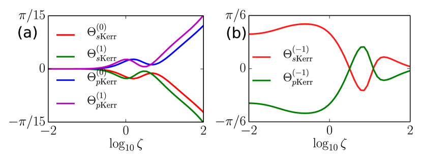
Figure 8: Kerr angle for $s$ and $p$ component of pump, probe and the new sideband, as a function of $\log_{10}\zeta$. Other parameters are same as those of Fig. 5.

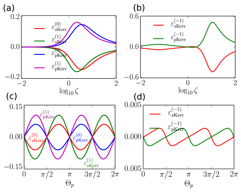
Figure 9: Ellipticity for $s$ and $p$ component as a function of $\log_{10}\zeta$ for (a) the pump and probe frequencies, and (b) the new sideband. Dependence of ellipticity for $s$ and $p$ component as a function of $\Theta_{p}$ for (c) the pump and probe frequencies, and (d) the new sideband. Here $\Theta_{p}=\pi/4$ for (a) and (b) and $\zeta=1$ for (c) and (d). Other parameters are same as those of Fig. 5.

In the non-linear response regime of $\zeta\geq 1$, we also find the transverse optical conductivity ($\sigma_{xy}$) to be finite depending on the value of $\Theta_{p}$. The expressions for $\sigma_{xy\boldsymbol{k}}$ for pump, probe and the new sideband can be obtained directly from Eq. (45), Eq. (47) and Eq. (49), respectively, by replacing $\sin^{2}{\phi_{\boldsymbol{k}}}\to-\sin{\phi_{\boldsymbol{k}}}\cos{\phi_{\boldsymbol{k}}}$. The pump field intensity and polarization dependence of the transverse optical conductivity for graphene is shown in Fig. 7. Note that these are in general smaller than the corresponding longitudinal counterparts.

The presence of a finite optical conductivity also leads to polarization rotation in the reflected and transmitted optical beams. In particular, for the reflected beam, the Kerr angle is given by given by Yoshino (2013); Singh et al. (2018b),

$$\Theta^{(\lambda)}_{s/p{\rm Kerr}}=\frac{1}{2}\tan^{-1}\left(\frac{2{{\rm Re}[\chi^{(\lambda)}_{s/p{\rm Kerr}}]}}{1-|\chi^{(\lambda)}_{s/p{\rm Kerr}}|^{2}}\right).$$ (50)

Here, $\lambda$ takes value $0$, $1$ and $-1$ for pump, probe and the new sideband frequencies, respectively. The explicit expressions for the $\chi_{s/p{\rm Kerr}}$ are given in Table I of the main manuscript. The dependence of the polarization rotation angle on the intensity of the pump beam is shown in Fig. 8. Evidently, the polarization angle of the newly generated optical sideband is significantly larger than the polarization rotation of the pump and probe fields.

The corresponding ellipticity of the reflected beam is expressed as,

$$\varepsilon^{(\lambda)}_{s/p{\rm Kerr}}=\tan\left[\frac{1}{2}\sin^{-1}\left(\frac{2{{\rm Im}[\chi^{(\lambda)}_{s/p{\rm Kerr}}]}}{1+|\chi^{(\lambda)}_{s/p{\rm Kerr}}|^{2}}\right)\right].$$ (51)

The pump field and polarization angle dependence of the ellipticity of the reflected optical fields at pump, probe and sideband frequencies is shown in Fig. 9.

References

- Hafez et al. (2018) Hassan A. Hafez, Sergey Kovalev, Jan-Christoph Deinert, Zoltán Mics, Bertram Green, Nilesh Awari, Min Chen, Semyon Germanskiy, Ulf Lehnert, Jochen Teichert, Zhe Wang, Klaas-Jan Tielrooij, Zhaoyang Liu, Zongping Chen, Akimitsu Narita, Klaus Müllen, Mischa Bonn, Michael Gensch, and Dmitry Turchinovich, “Extremely efficient terahertz high-harmonic generation in graphene by hot dirac fermions,” Nature 561, 507–511 (2018).
- Yoshikawa et al. (2017) Naotaka Yoshikawa, Tomohiro Tamaya, and Koichiro Tanaka, “Optics: High-harmonic generation in graphene enhanced by elliptically polarized light excitation,” Science 356, 736–738 (2017).
- Prechtel et al. (2012) Leonhard Prechtel, Li Song, Dieter Schuh, Pulickel Ajayan, Werner Wegscheider, and Alexander W. Holleitner, “Time-resolved ultrafast photocurrents and terahertz generation in freely suspended graphene,” Nature Communications 3, 646 (2012).
- Jiang et al. (2018) Tao Jiang, Di Huang, Jinluo Cheng, Xiaodong Fan, Zhihong Zhang, Yuwei Shan, Yangfan Yi, Yunyun Dai, Lei Shi, Kaihui Liu, Changgan Zeng, Jian Zi, J. E. Sipe, Yuen Ron Shen, Wei Tao Liu, and Shiwei Wu, “Gate-tunable third-order nonlinear optical response of massless Dirac fermions in graphene,” Nature Photonics 12, 430–436 (2018).
- Gu et al. (2012) T. Gu, N. Petrone, J. F. McMillan, A. Van Der Zande, M. Yu, G. Q. Lo, D. L. Kwong, J. Hone, and C. W. Wong, “Regenerative oscillation and four-wave mixing in graphene optoelectronics,” Nature Photonics 6, 554–559 (2012).
- Hendry et al. (2010) E. Hendry, P. J. Hale, J. Moger, A. K. Savchenko, and S. A. Mikhailov, “Coherent nonlinear optical response of graphene,” Phys. Rev. Lett. 105, 097401 (2010).
- Yang et al. (2011) Hongzhi Yang, Xiaobo Feng, Qian Wang, Han Huang, Wei Chen, Andrew T. S. Wee, and Wei Ji, “Giant two-photon absorption in bilayer graphene,” Nano Letters 11, 2622–2627 (2011).
- Zhang et al. (2012) Han Zhang, Stéphane Virally, Qiaoliang Bao, Loh Kian Ping, Serge Massar, Nicolas Godbout, and Pascal Kockaert, “Z-scan measurement of the nonlinear refractive index of graphene,” Opt. Lett. 37, 1856–1858 (2012).
- Kumar et al. (2013) Nardeep Kumar, Jatinder Kumar, Chris Gerstenkorn, Rui Wang, Hsin-Ying Chiu, Arthur L. Smirl, and Hui Zhao, “Third harmonic generation in graphene and few-layer graphite films,” Phys. Rev. B 87, 121406 (2013).
- Hong et al. (2013) Sung-Young Hong, Jerry I. Dadap, Nicholas Petrone, Po-Chun Yeh, James Hone, and Richard M. Osgood, “Optical third-harmonic generation in graphene,” Phys. Rev. X 3, 021014 (2013).
- Mikhailov and Ziegler (2008) S. A. Mikhailov and K. Ziegler, “Nonlinear electromagnetic response of graphene: frequency multiplication and the self-consistent-field effects,” Journal of Physics: Condensed Matter 20, 384204 (2008).
- Glazov and Ganichev (2014) M. M. Glazov and S. D. Ganichev, “High frequency electric field induced nonlinear effects in graphene,” Physics Reports 535, 101–138 (2014).
- Cheng et al. (2014) J L Cheng, N Vermeulen, and J E Sipe, “Third order optical nonlinearity of graphene,” New Journal of Physics 16, 053014 (2014).
- Al-Naib et al. (2014) Ibraheem Al-Naib, J. E. Sipe, and Marc M. Dignam, “High harmonic generation in undoped graphene: Interplay of inter- and intraband dynamics,” Phys. Rev. B 90, 245423 (2014).
- Tamaya et al. (2016a) T. Tamaya, A. Ishikawa, T. Ogawa, and K. Tanaka, “Diabatic mechanisms of higher-order harmonic generation in solid-state materials under high-intensity electric fields,” Phys. Rev. Lett. 116, 016601 (2016a).
- Cheng et al. (2015) J. L. Cheng, N. Vermeulen, and J. E. Sipe, “Third-order nonlinearity of graphene: Effects of phenomenological relaxation and finite temperature,” Phys. Rev. B 91, 235320 (2015).
- Mikhailov (2016) S. A. Mikhailov, “Quantum theory of the third-order nonlinear electrodynamic effects of graphene,” Phys. Rev. B 93, 085403 (2016).
- Rostami and Polini (2016) Habib Rostami and Marco Polini, “Theory of third-harmonic generation in graphene: A diagrammatic approach,” Phys. Rev. B 93, 161411 (2016).
- Gullans et al. (2013) M. Gullans, D. E. Chang, F. H. L. Koppens, F. J. G. de Abajo, and M. D. Lukin, “Single-photon nonlinear optics with graphene plasmons,” Phys. Rev. Lett. 111, 247401 (2013).
- Yao et al. (2014) Xianghan Yao, Mikhail Tokman, and Alexey Belyanin, “Efficient nonlinear generation of thz plasmons in graphene and topological insulators,” Phys. Rev. Lett. 112, 055501 (2014).
- Crosse et al. (2014) J. A. Crosse, Xiaodong Xu, Mark S. Sherwin, and R. B. Liu, “Theory of low-power ultra-broadband terahertz sideband generation in bi-layer graphene,” Nature Communications 5, 4854 (2014).
- Cox et al. (2017) Joel D. Cox, Andrea Marini, and F. Javier Garcia de Abajo, “Plasmon-assisted high-harmonic generation in graphene,” Nature Communications 8, 14380 (2017).
- Bonaccorso et al. (2010) F. Bonaccorso, Z. Sun, T. Hasan, and A. C. Ferrari, “Graphene photonics and optoelectronics,” Nature Photonics 4, 611–622 (2010).
- Bao and Loh (2012) Qiaoliang Bao and Kian Ping Loh, “Graphene photonics, plasmonics, and broadband optoelectronic devices,” ACS Nano 6, 3677–3694 (2012).
- Tamaya et al. (2016b) T. Tamaya, A. Ishikawa, T. Ogawa, and K. Tanaka, “Higher-order harmonic generation caused by elliptically polarized electric fields in solid-state materials,” Phys. Rev. B 94, 241107 (2016b).
- Dawlaty et al. (2008) Jahan M. Dawlaty, Shriram Shivaraman, Mvs Chandrashekhar, Farhan Rana, and Michael G. Spencer, “Measurement of ultrafast carrier dynamics in epitaxial graphene,” Applied Physics Letters 92, 042116 (2008).
- Johannsen et al. (2013) Jens Christian Johannsen, Søren Ulstrup, Federico Cilento, Alberto Crepaldi, Michele Zacchigna, Cephise Cacho, I. C. Edmond Turcu, Emma Springate, Felix Fromm, Christian Raidel, Thomas Seyller, Fulvio Parmigiani, Marco Grioni, and Philip Hofmann, “Direct view of hot carrier dynamics in graphene,” Phys. Rev. Lett. 111, 027403 (2013).
- Boyd (2008) R.W. Boyd, Nonlinear Optics, Nonlinear Optics Series (Elsevier Science, 2008).
- Schubert et al. (2014) O. Schubert, M. Hohenleutner, F. Langer, B. Urbanek, C. Lange, U. Huttner, D. Golde, T. Meier, M. Kira, S. W. Koch, and R. Huber, “Sub-cycle control of terahertz high-harmonic generation by dynamical Bloch oscillations,” Nature Photonics 8, 119–123 (2014).
- Zhang and Voss (2011) Zheshen Zhang and Paul L. Voss, “Full-band quantum-dynamical theory of saturation and four-wave mixing in graphene,” Opt. Lett. 36, 4569–4571 (2011).
- Burghoff et al. (2014) David Burghoff, Tsung-Yu Kao, Ningren Han, Chun Wang Ivan Chan, Xiaowei Cai, Yang Yang, Darren J. Hayton, Jian-Rong Gao, John L. Reno, and Qing Hu, “Terahertz laser frequency combs,” Nature Photonics 8, 462–467 (2014).
- Aversa and Sipe (1995) Claudio Aversa and J. E. Sipe, “Nonlinear optical susceptibilities of semiconductors: Results with a length-gauge analysis,” Phys. Rev. B 52, 14636–14645 (1995).
- Singh et al. (2017) Ashutosh Singh, Kirill I. Bolotin, Saikat Ghosh, and Amit Agarwal, “Nonlinear optical conductivity of a generic two-band system with application to doped and gapped graphene,” Phys. Rev. B 95, 155421 (2017).
- Singh et al. (2018a) Ashutosh Singh, Saikat Ghosh, and Amit Agarwal, “Nonlinear, anisotropic, and giant photoconductivity in intrinsic and doped graphene,” Phys. Rev. B 97, 045402 (2018a).
- Singh et al. (2018b) Ashutosh Singh, Saikat Ghosh, and Amit Agarwal, “Nonlinear and anisotropic polarization rotation in two-dimensional dirac materials,” Phys. Rev. B 97, 205420 (2018b).
- Chaves et al. (2016) A. J. Chaves, N. M. R. Peres, and Tony Low, “Pumping electrons in graphene to the point in the brillouin zone: Emergence of anisotropic plasmons,” Phys. Rev. B 94, 195438 (2016).
- Note (1) Strictly speaking, there is an additional term of the form on the right hand side of Eq. (16\@@italiccorr). However this term can be safely neglected as it 1) oscillates with a frequency Singh et al. (2017) and 2) its impact on the final steady state dynamics turns out to be very small Singh et al. (2018b).
- Semnani et al. (2018) Behrooz Semnani, Roland Jago, Safieddin Safavi-Naeini, Amir Hamed Majedi, Ermin Malic, and Philippe Tassin, “Anomalous optical saturation of low-energy Dirac states in graphene and its implication for nonlinear optics,” arXiv e-prints , arXiv:1806.10123 (2018), arXiv:1806.10123 [cond-mat.mes-hall] .
- Yoshino (2013) Toshihiko Yoshino, “Theory for oblique-incidence magneto-optical faraday and kerr effects in interfaced monolayer graphene and their characteristic features,” J. Opt. Soc. Am. B 30, 1085–1091 (2013).
- Note (2) The simplified expressions in the last column are obtained using , along with – which works in the case of graphene.
- Nair et al. (2008) R. R. Nair, P. Blake, A. N. Grigorenko, K. S. Novoselov, T. J. Booth, T. Stauber, N. M. R. Peres, and A. K. Geim, “Fine structure constant defines visual transparency of graphene,” Science 320, 1308 (2008).
- Mak et al. (2008) Kin Fai Mak, Matthew Y. Sfeir, Yang Wu, Chun Hung Lui, James A. Misewich, and Tony F. Heinz, “Measurement of the optical conductivity of graphene,” Phys. Rev. Lett. 101, 196405 (2008).
- Note (3) Reflectivity and polarization rotation for the newly generated sideband are defined in reference to the amplitude of backward propagating field , and its polarization relative to the polarization of the incident pump beam.
- Katsnelson (2012) M. I. Katsnelson, Graphene: Carbon in Two Dimensions (Cambridge University Press, 2012).