On the Termination Problem
for Probabilistic Higher-Order Recursive Programs

Abstract.

In the last two decades, there has been much progress on model checking of both probabilistic systems and higher-order programs. In spite of the emergence of higher-order probabilistic programming languages, not much has been done to combine those two approaches. In this paper, we initiate a study on the probabilistic higher-order model checking problem, by giving some first theoretical and experimental results. As a first step towards our goal, we introduce PHORS, a probabilistic extension of higher-order recursion schemes (HORS), as a model of probabilistic higher-order programs. The model of PHORS may alternatively be viewed as a higher-order extension of recursive Markov chains. We then investigate the probabilistic termination problem — or, equivalently, the probabilistic reachability problem. We prove that almost sure termination of order-2 PHORS is undecidable. We also provide a fixpoint characterization of the termination probability of PHORS, and develop a sound (although possibly incomplete) procedure for approximately computing the termination probability. We have implemented the procedure for order-2 PHORS, and confirmed that the procedure works well through preliminary experiments.

1. Introduction

Computer science has interacted with probability theory in many fruitful ways, since the very early days [dLMSS56]. Probability theory enables state abstraction, reducing in this way the state space’s cardinality. It has also led to a new model of computation, used for instance in randomized computation [MR95] or in cryptography [GM84]. The trend of a rise of probability theory’s importance in computer science has been followed by the programming language community, up to the point that probabilistic programming is nowadays a very active research area. Probabilistic choice can be modeled in various ways in programming, and fair binary probabilistic choice is for instance perfectly sufficient to obtain universality if the underlying programming language is universal itself [San69, DZ12]. This has been the path followed in probabilistic $\lambda$-calculi [Sah78, JP89, DH02, DZ12, ETP14, DSA14, HKSY17].

In the present paper, we are interested in the analysis of probabilistic, higher-order recursive programs. Model checking of probabilistic finite state systems has been a very active research field (see [BK08, CHVB18] for a survey). Over the last two decades, there has also been much interest and progress in model checking of probabilistic recursive programs [EY09, EY15, BEKK13, BBFK14], which cannot be modeled as finite state systems, and thus escape the classic model checking framework and algorithms. None of the proposals in the literature on probabilistic model checking, however, is capable of handling higher-order functions, which are a natural feature in functional languages. This is in sharp contrast with what happens for non-probabilistic higher-order programs, for which model checking techniques can be fruitfully employed for proving both reachability and safety properties, as shown in the extensive literature on the subject (e.g. [Ong06, HMOS08, Kob13, KO09, KSU11, GM15b, GM15a, TO14, SW11]). There have been some studies on the termination of probabilistic higher-order programs [DLG17], but to our knowledge, they have not provided a procedure for precisely computing the termination probability, nor discussed whether it is possible at all: see Section 7 for more details. Summing up, little has been known about the decidability and complexity of model checking of probabilistic higher-order programs, and even less about the existence of practical procedures for approximately solving model checking problems.

One may think that probabilistic and higher-order computation is rather an exotic research topic, but it is important for precisely modeling and verifying any higher-order functional programs that interact with a probabilistic environment. As a simple example, consider the following (non-higher-order) OCaml-like program, which uses a primitive flip for generating true or false with probability $\frac{1}{2}$.

⬇

let rec f() = if flip() then () else f() in f()

The program almost surely terminates (i.e., terminates with probability 1), but if we ignore the probabilistic aspects and model flip() as a non-deterministic (rather than probabilistic) primitive, then we would conclude that the program can may diverge. The following program makes use of an interesting combination of probabilistic choice and higher-order functions:

⬇

let boolgen() = flip()

let rec listgen f () =

if flip() then [] else f()::listgen f ()

in listgen (listgen boolgen) ()

The function listgen above takes a generator f of elements as an argument, and creates a list of elements, each of them obtained by calling $f$. Thus, the whole program generates a list of lists of Booleans. The length of such a list of lists is randomized, and distributed according to the geometric distribution. We may then wish to ask, for example, (i) whether it almost surely terminates, and (ii) what is the probability that a list of even length is generated. Generating random data structures like the one produced by listgen is not an artificial task, being central to, e.g., random test generation [PF17, MRH18].

As a model of probabilistic higher-order programs, we first introduce PHORS, a probabilistic extension of higher-order recursion schemes (HORS) [KNU02, Ong06]. Our model of PHORS is expressive enough to accurately model probabilistic higher-order functions, but the underlying non-probabilistic language (i.e., HORS, obtained by removing probabilistic choice) is not Turing-complete; thus, we can hope for the existence of algorithmic solutions to some of the verification problems. As an example, we can decide indeed whether the termination probability of PHORS is $0$, by reduction to a model checking problem for non-probabilistic HORS.

Through the well-known correspondence between HORS and (collapsible) higher-order pushdown automata [KNU02, HMOS08], PHORS can be considered a higher-order extension of probabilistic pushdown systems [BEKK13, BBFK14] and of recursive Markov chains [YE05], the computation models used in previous work on model checking of probabilistic recursive programs. We can also view PHORS as an extension of the $\lambda Y$-calculus [Sta04] with probabilities, just like HORS can be viewed as an alternative presentation of the $\lambda Y$-calculus. The correspondence between HORS and the $\lambda Y$-calculus has been useful for transferring techniques for typed $\lambda$-calculi (most notably, game semantics [Ong06], intersection types [Kob09b, KO09] and Krivine machines [SW11]) to HORS; thus, we expect similar benefits in using PHORS (rather than probabilistic higher-order pushdown automata) as models of probabilistic higher-order programs.

As a first step towards understanding the nature of the model checking problem for probabilistic higher-order programs, the present paper studies the problem of computing the termination (or equivalently, reachability) probabilities of PHORS. Note that, as in a non-probabilistic setting, one can easily reduce a safety property verification problem to a may-termination problem (i.e. the problem of checking whether a program may terminate), by encoding safety violation as termination. We can also verify certain liveness properties, by encoding a good event as a termination and checking that the termination probability is $1$. As we will see in Section 2, the two questions (i) and (ii) mentioned earlier on the listgen program can also be reduced to the problem of computing the termination probability of a PHORS. Note also that computing the termination (or equivalently, reachability) probability has been a key to solving more general model checking problems (such as LTL/CTL model checking) for recursive programs [YE05, BBFK14].

As the first result on the problem of computing termination probabilities, we prove that the almost sure termination problem, i.e., whether a given PHORS terminates with probability $1$, is undecidable at order-2 or higher. This contrasts with the case of recursive Markov chains, for which the almost sure termination problem can be decided in PSPACE [EY09]. The proof of undecidability is based on a reduction from the undecidability of Hilbert’s tenth problem (i.e. unsolvability of Diophantine equations) [Mat93]. The undecidability result also implies that it is not possible to compute the exact termination probability. More precisely, for any rational number $r\in(0,1]$, the set $\{\mathcal{G}\mid\Pr(\mathcal{G})\geq r\}$ (where $\Pr(\mathcal{G})$ denotes the termination probability of $\mathcal{G}$) is not recursively enumerable (in other words, the set is $\Pi^{0}_{\_}1$-hard in the arithmetical hierarchy). Note, however, that this negative result does not preclude the possibility to compute the termination probability with arbitrary precision; there may exist an algorithm that, given a PHORS $\mathcal{G}$ and $\epsilon>0$ as inputs, finds $r$ such that the termination probability of $\mathcal{G}$ belongs to $(r,r+\epsilon)$. The existence of such an approximation algorithm remains open.

As a positive result towards approximately computing the termination probability, we show that the termination probability of order-$n$ PHORS can be characterized by fixpoint equations on order-($n-1$) functions on real numbers. The fixpoint characterization of the termination probability of recursive Markov chains [EY09] can be viewed as a special case of our result where $n=1$. The fixpoint characterization immediately provides a semi-algorithm for the lower-bound problem: “Given a PHORS $\mathcal{G}$ and a rational number $r\in[0,1]$, does $\Pr(\mathcal{G})>r$ hold?” Recall, however, that $\{\mathcal{G}\mid\Pr(\mathcal{G})\geq r\}$ is not recursively enumerable, so there is no semi-algorithm for the variation: “Given a PHORS $\mathcal{G}$ and a rational number $r\in[0,1]$, does $\Pr(\mathcal{G})\geq r$ hold?”

The remaining question is whether an upper-bound on the termination probability can be computed with arbitrary precision. We have not settled this question yet, but propose a procedure for soundly estimating an upper-bound of the termination probability of order-2 PHORS by using the fixpoint characterization above, à la FEM (finite element method). We have implemented the procedure, and conducted preliminary experiments to confirm that the procedure works fairly well in practice: combined with the lower-bound computation based on the fixpoint characterization, the procedure was able to instantly compute the termination probabilities of (small but) non-trivial examples with precision $10^{-2}$. We also briefly discuss how to generalize the procedure to deal with PHORS of arbitrary orders.

The contributions of this article can thus be summarized as follows:

1. A formalization of probabilistic higher-order recursion schemes (PHORS) and their termination probabilities. This is in Section 2.

2. A proof of undecidability of the almost sure termination problem for PHORS (of order 2 or higher), which can be found in Section 3.

3. A fixpoint characterization of the termination probability of PHORS, which immediately yields the semi-decidability of the lower-bound problem. This is in Section 4.

4. A sound procedure for computing an upper-bound to the termination probability of order-2 PHORS (which is described in Section 5) accompanied by an implementation and preliminary experiments with promising results, reported in Section 6.

We also discuss related work in Section 7, and conclude the article in Section 8. A preliminary summary of this article appeared in Proceedings of LICS 2019 [KDLG19].

2. Probabilistic Higher-Order Recursion Schemes (PHORS) and Termination Probabilities

This section introduces probabilistic higher-order recursion schemes (PHORS), an extension of higher-order recursion schemes [KNU02, Ong06] in which programs can at any evaluation step perform a discrete probabilistic choice, then proceeding according to its outcome. Higher-order recursion schemes are usually treated as generators of infinite trees, but as we are only interested in the termination probability, we consider only nullary tree constructors $\mathtt{e}$ and $\Omega$, which represent termination and divergence respectively.

We first define types and applicative terms. The set of types, ranged over by $\kappa$, is given by:

$$\kappa::=\mathtt{o}\mid\kappa_{\_}1\to\kappa_{\_}2.$$

Intuitively, $\mathtt{o}$ describes the unit value, and $\kappa_{\_}1\to\kappa_{\_}2$ describes functions from $\kappa_{\_}1$ to $\kappa_{\_}2$. As usual, the order of a type $\kappa$ is defined by:

$$\mathit{order}(\mathtt{o}) =0$$

$$\mathit{order}(\kappa_{\_}1\to\kappa_{\_}2) =\max(\mathit{order}(\kappa_{\_}1)+1,\mathit{order}(\kappa_{\_}2)).$$

We often write $\mathtt{o}^{\ell}\to\mathtt{o}$ for $\underbrace{\mathtt{o}\to\cdots\to\mathtt{o}}_{\_}\ell\to\mathtt{o}$, and abbreviate $\kappa_{\_}1\to\cdots\to\kappa_{\_}k\to\kappa$ to $\widetilde{\kappa}\to\kappa$. The set of applicative terms, ranged over by $t$, is given by:

$$t::=\mathtt{e}\ \;\;\mbox{\Large{$\mid$}}\;\;\Omega\;\;\mbox{\Large{$\mid$}}\;\;\ x\ \;\;\mbox{\Large{$\mid$}}\;\;\ t_{\_}1t_{\_}2,$$

where $\mathtt{e}$ and $\Omega$ are (the only) constants of type $\mathtt{o}$ and $x$ ranges over a set of variables. Intuitively, $\mathtt{e}$ and $\Omega$ denote termination and divergence respectively (the latter can be defined as a derived form, but assuming it as a primitive is convenient for Section 4). We consider the following standard simple type system for applicative terms, where $\mathcal{K}$, called a type environment, is a map from a finite set of variables to the set of types.

$$\mathcal{K}\vdash\mathtt{e}:\mathtt{o}\qquad\qquad\mathcal{K}\vdash\Omega:\mathtt{o}\qquad\qquad\mathcal{K}\vdash x\mathbin{:}\kappa\mathcal{K}(x)=\kappa\qquad\qquad\mathcal{K}\vdash t_{\_}1t_{\_}2:\kappa\mathcal{K}\vdash t_{\_}1:\kappa_{\_}2\to\kappa\quad\quad\mathcal{K}\vdash t_{\_}2:\kappa_{\_}2$$

Definition (PHORS).

A probabilistic higher-order recursion scheme (PHORS) is a triple $\mathcal{G}=(\mathcal{N},\mathcal{R},S)$, where:

1. $\mathcal{N}$ is a map from a finite set of variables (called non-terminals and typically denoted $F,\,G,\,\ldots$) to the set of types.

2. $\mathcal{R}$ is a map from $\mathit{dom}(\mathcal{N})$ to terms of the form $\lambda x_{\_}1.\cdots\lambda x_{\_}k.t_{\_}L\,\oplus_{p}\,t_{\_}R$, where $p\in[0,1]$ is a rational number, and $t_{\_}L,\,t_{\_}R$ are applicative terms. If $\mathcal{N}(F)=\kappa_{\_}1\to\cdots\to\kappa_{\_}k\to\mathtt{o}$, $\mathcal{R}(F)$ must be of the form $\lambda x_{\_}1.\cdots\lambda x_{\_}k.t_{\_}L\,\oplus_{p}\,t_{\_}R$, where $\mathcal{N},x_{\_}1\mathbin{:}\kappa_{\_}1,\ldots,x_{\_}k\mathbin{:}\kappa_{\_}k\vdash t_{\_}L:\mathtt{o}$ and $\mathcal{N},x_{\_}1\mathbin{:}\kappa_{\_}1,\ldots,x_{\_}k\mathbin{:}\kappa_{\_}k\vdash t_{\_}R:\mathtt{o}$.

3. $S\in\mathit{dom}(\mathcal{N})$, called the start symbol, is a distinguished non-terminal that satisfies $\mathcal{N}(S)=\mathtt{o}$.

The order of a PHORS $(\mathcal{N},\mathcal{R},S)$ is $\max_{\_}{F\in\mathit{dom}(\mathcal{N})}\mathit{order}(\mathcal{N}(F))$, i.e., the highest order of the types of its non-terminals. We write $\mathcal{P}_{\_}k$ for the set of order-$k$ PHORS.

When $\mathcal{R}(F)=\lambda x_{\_}1.\cdots\lambda x_{\_}k.t_{\_}L\,\oplus_{p}\,t_{\_}R$, we often write $F\,x_{\_}1\,\cdots\,x_{\_}k=t_{\_}L\,\oplus_{p}\,t_{\_}R$, and specify $\mathcal{R}$ as a set of such equations. The rule $F\,x_{\_}1\,\cdots\,x_{\_}k=t_{\_}L\,\oplus_{p}\,t_{\_}R$ intuitively means that $F\,t_{\_}1\,\cdots\,t_{\_}k$ is reduced to $[t_{\_}1/x_{\_}1,\ldots,t_{\_}k/x_{\_}k]t_{\_}L$ and $[t_{\_}1/x_{\_}1,\ldots,t_{\_}k/x_{\_}k]t_{\_}R$ with probabilities $p$ and $1-p$, respectively. We often write just $F\,x_{\_}1\,\cdots\,x_{\_}k=t_{\_}L$ for $F\,x_{\_}1\,\cdots\,x_{\_}k=t_{\_}L\,\oplus_{1}\,t_{\_}R$.

Definition (Operational Semantics and Termination Probability of PHORS).

Given a PHORS $\mathcal{G}=(\mathcal{N},\mathcal{R},S)$, the rewriting relation $\xrightarrow{d,p}_{\mathcal{G}}$ (where $d\in\{L,R\}$ and $p\in[0,1]$) is defined by:

$$F\,t_{\_}1\,\cdots\,t_{\_}k\xrightarrow{L,p}_{\mathcal{G}}[t_{\_}1/x_{\_}1,\ldots,t_{\_}k/x_{\_}k]t_{\_}{L}\mathcal{R}(F)=\lambda x_{\_}1.\cdots\lambda x_{\_}k.t_{\_}L\,\oplus_{p}\,t_{\_}R\qquad\qquad F\,t_{\_}1\,\cdots\,t_{\_}k\xrightarrow{R,1-p}_{\mathcal{G}}[t_{\_}1/x_{\_}1,\ldots,t_{\_}k/x_{\_}k]t_{\_}{R}\mathcal{R}(F)=\lambda x_{\_}1.\cdots\lambda x_{\_}k.t_{\_}L\,\oplus_{p}\,t_{\_}R$$

We write $\ext@arrow 0359\Rightarrowfill@{}{\pi,p}_{\mathcal{G}}$ for the relational composition of $\xrightarrow{d_{\_}1,p_{\_}1}_{\mathcal{G}},\ldots,\xrightarrow{d_{\_}n,p_{\_}n}_{\mathcal{G}}$, when $\pi=d_{\_}1\cdots d_{\_}n$ and $p=\prod_{\_}{i=1}^{n}p_{\_}i$. Note that $n$ may be $0$, so that we have $t_{\_}1\ext@arrow 0359\Rightarrowfill@{}{\epsilon,1}_{\mathcal{G}}t_{\_}2$ iff $t_{\_}1=t_{\_}2$. By definition, for each $\pi\in\{L,R\}^{*}$, there exists at most one $p$ such that $S\ext@arrow 0359\Rightarrowfill@{}{\pi,p}_{\mathcal{G}}\ \!\mathtt{e}$. For an applicative term $t$, we define $\mathcal{P}(\mathcal{G},t,\pi)$ by:

$$\mathcal{P}(\mathcal{G},t,\pi)=\left\{\begin{array}[]{ll}p&\mbox{if $t\ext@arrow 0359\Rightarrowfill@{}{\pi,p}_{\mathcal{G}}\mathtt{e}$}\\ 0&\mbox{if $t\ext@arrow 0359\Rightarrowfill@{}{\pi,p}_{\mathcal{G}}\mathtt{e}$ does not hold for any $p$}\end{array}\right..$$

The partial and full termination probabilities, written $\mathcal{P}(\mathcal{G},t,n)$ and $\mathcal{P}(\mathcal{G},t)$, are defined by:

$$\mathcal{P}(\mathcal{G},t,n)=\displaystyle\sum_{\_}{\pi\in\{L,R\}^{\leq n}}\ \ \mathcal{P}(\mathcal{G},t,\pi)\qquad\text{and}\qquad\mathcal{P}(\mathcal{G},t)=\displaystyle\sum_{\_}{\pi\in\{L,R\}^{*}}\ \ \mathcal{P}(\mathcal{G},t,\pi).$$

Finally, we set $\mathcal{P}(\mathcal{G},n)\,=\,\mathcal{P}(\mathcal{G},S,n)$ and $\mathcal{P}(\mathcal{G})\,=\,\mathcal{P}(\mathcal{G},S)$.

We often omit the subscript $\mathcal{G}$ below and just write $\xrightarrow{d,p}$ and $\ext@arrow 0359\Rightarrowfill@{}{\pi,p}$ for $\xrightarrow{d,p}_{\mathcal{G}}$ and $\ext@arrow 0359\Rightarrowfill@{}{\pi,p}_{\mathcal{G}}$ respectively. The termination probability of $\mathcal{G}$ refers to its full termination probability $\mathcal{P}(\mathcal{G})$.

Example 2.1.

Let $\mathcal{G}_{\_}1$ be the order-1 PHORS $(\mathcal{N}_{\_}1,\mathcal{R}_{\_}1,S)$, where:

$$\begin{array}[]{l}\mathcal{N}_{\_}1=\{S\mapsto\mathtt{o},F\mapsto\mathtt{o}\to\mathtt{o}\}\\ \mathcal{R}_{\_}1=\{S\ =\ F\,\mathtt{e}\,\oplus_{1}\,\Omega,\quad F\,x\ =\ x\,\oplus_{p}\,F(F\,x)\}.\end{array}$$

The start symbol $S$ can be reduced, for example, as follows.

$$S\xrightarrow{L,1}F(\mathtt{e})\xrightarrow{R,1-p}F(F\,\mathtt{e})\xrightarrow{L,p}F\,\mathtt{e}\xrightarrow{L,p}\mathtt{e}.$$

Thus, we have $S\ext@arrow 0359\Rightarrowfill@{}{LRLL,p^{2}(1-p)}_{\,}\!\mathtt{e}$. As we will see in Section 4, the termination probability $\mathcal{P}(\mathcal{G}_{\_}1)$ is the least solution for $r$ of the fixpoint equation: $r=p+(1-p)r^{2}$. Therefore, $\mathcal{P}(\mathcal{G}_{\_}1)=\frac{p}{1-p}$ if $0\leq p<\frac{1}{2}$ and $\mathcal{P}(\mathcal{G}_{\_}1)=1$ if $\frac{1}{2}\leq p$. The corresponding example of a recursive Markov chain is shown in Figure 1, using the notational conventions from [EY09]. $\mathcal{G}_{\_}1$ can be seen as realizing a binary, random walk on the natural numbers, starting from $1$. ∎

Figure 1. A Recursive Markov Chain Modeling $\mathcal{G}_{\_}1$.

As the previous example suggests, there is a mutual translation between recursive Markov chains and order-1 PHORS; see the Appendix A.1 for details.

Example 2.2.

Let $\mathcal{G}_{\_}2$ be the order-2 PHORS $(\mathcal{N}_{\_}2,\mathcal{R}_{\_}2,S)$ where:

$$\mathcal{N}_{\_}2= \;\{S\mapsto\mathtt{o},H\mapsto\mathtt{o}\to\mathtt{o},F\mapsto(\mathtt{o}\to\mathtt{o})\to\mathtt{o},$$

$$\hskip 8.00003ptD\mapsto(\mathtt{o}\to\mathtt{o})\to\mathtt{o}\to\mathtt{o}\}$$

$$\mathcal{R}_{\_}2= \;\{S=\ (F\,H)\,\oplus_{1}\,\mathtt{e},\ H\,x=x\,\oplus_{\frac{1}{2}}\,\Omega,$$

$$\hskip 8.00003ptF\,g=(g\,\mathtt{e})\,\oplus_{\frac{1}{2}}\,(F(D\,g)),\ D\,g\,x=(g\,(g\,x))\,\oplus_{1}\,\Omega\}.$$

The start symbol $S$ can be reduced, for example, as follows.

$$S \xrightarrow{L,1}F\,H\xrightarrow{R,\frac{1}{2}}F(D\,H)\xrightarrow{L,\frac{1}{2}}D\,H\,\mathtt{e}\xrightarrow{L,1}H(H\,\mathtt{e})$$

$$\xrightarrow{L,\frac{1}{2}}H\,\mathtt{e}\xrightarrow{L,\frac{1}{2}}\mathtt{e}.$$

Contrary to $\mathcal{G}_{\_}1$, it is quite hard to find an RMC which models the behavior of $\mathcal{G}_{\_}2$. In fact, this happens for very good reasons, as we will see in Section 3. ∎

The following result is obvious from the definition of $\mathcal{P}(\mathcal{G})$.

Theorem 2.2.

For any rational number $r\in[0,1]$, the set $\{\mathcal{G}\mid\mathcal{P}(\mathcal{G})>r\}$ is recursively enumerable.

Proof 2.3.

This follows immediately from the facts that $\mathcal{P}(\mathcal{G})>r$ if and only if $\mathcal{P}(\mathcal{G},n)=\sum_{\_}{\pi\in\{L,R\}^{\leq n}}\,\mathcal{P}(\mathcal{G},S,\pi)>r$ for some $n$, and that $\mathcal{P}(\mathcal{G},n)$ is computable.

In other words, whether $\mathcal{P}(\mathcal{G})>r$ is semi-decidable, i.e., there exists a procedure that eventually answers “yes” whenever $\mathcal{P}(\mathcal{G})>r$. As we will see in Section 3, however, for every $r\in(0,1]$, $\{\mathcal{G}\mid\mathcal{P}(\mathcal{G})\geq r\}$ is not recursively enumerable.

Remark 2.4.

Given a PHORS $\mathcal{G}$, replacing each probabilistic operator $\,\oplus_{p}\,$ s.t. $0<p<1$ with a binary tree constructor br and replacing $t_{\_}L\,\oplus_{1}\,t_{\_}R$ ($t_{\_}L\,\oplus_{0}\,t_{\_}R$, resp.) with $t_{\_}L$ ($t_{\_}R$, resp.), we obtain an ordinary HORS $\mathcal{G}^{\mathit{ND}}$. Then $\mathcal{P}(\mathcal{G})=0$ if and only if the tree generated by $\mathcal{G}^{\mathit{ND}}$ has no finite path to $\mathtt{e}$. Thus, by [KO11] (see the paragraph below the proof of Theorem 4.5 about the complexity of the reachability problem), whether $\mathcal{P}(\mathcal{G})=0$ is decidable, and $(n-1)$-EXPTIME complete. Note, on the other hand, that there is no clear correspondence between the almost sure termination problem $\mathcal{P}(\mathcal{G})\stackrel{{\scriptstyle?}}{{=}}1$ and a model checking problem for $\mathcal{G}^{\mathit{ND}}$. If the tree of $\mathcal{G}^{\mathit{ND}}$ has neither $\Omega$ nor an infinite path (which is decidable), then $\mathcal{P}(\mathcal{G}){=}1$, but the converse does not hold.

Remark 2.5.

The restriction that a probabilistic choice may occur only at the top-level of each rule is not a genuine restriction. Indeed, whenever we wish to write a rule of the form $F\;\widetilde{x}=C[t_{\_}L\,\oplus_{p}\,t_{\_}R]$, we can normalize it to $F\;\widetilde{x}=C[G\;\widetilde{x}]$, where $G$ is defined by $G\;\widetilde{x}=t_{\_}L\,\oplus_{p}\,t_{\_}R$. Keeping this in mind, we sometimes allow probabilistic choices to occur inside terms. In fact, a PHORS can be considered as a term (of type $\mathtt{o}$) of a probabilistic extension of the (call-by-name) $\lambda Y$-calculus [Sta04]. We define the set of probabilistic $\lambda Y$ terms by:

$$s::=\mathtt{e}\;\;\mbox{\Large{$\mid$}}\;\;\Omega\;\;\mbox{\Large{$\mid$}}\;\;x\;\;\mbox{\Large{$\mid$}}\;\;\lambda x.s\;\;\mbox{\Large{$\mid$}}\;\;s_{\_}1s_{\_}2\;\;\mbox{\Large{$\mid$}}\;\;Y(\lambda f.\lambda x.s)\;\;\mbox{\Large{$\mid$}}\;\;s_{\_}1\,\oplus_{p}\,s_{\_}2.$$

Here, $\,\oplus_{p}\,$ is a probabilistic choice operator of type $\mathtt{o}\to\mathtt{o}\to\mathtt{o}$, and other terms are simply-typed in the usual way. Then, PHORS and probabilistic $\lambda Y$ terms can be converted to each other. We use PHORS in the present paper for the convenience of the fixpoint characterizations discussed in Section 4.

Remark 2.6.

We adopt the call-by-name semantics, and allow probabilistic choices only on terms of type $\mathtt{o}$. The call-by-value semantics, as well as probabilistic choices at higher-order types can be modeled by applying a standard CPS transformation. Moreover, a PHORS does not have data other than functions, but as in ordinary HORS [Kob13], elements of a finite set (such as Booleans) can be modeled by using Church encoding.

We provide a few more examples of PHORS below.

Example 2.7.

Recall the list generator example in Section 1, whose termination is equivalent to that of the following program, obtained by replacing the output of each function with the unit value ().

⬇

let boolgen() = flip() in

let rec listgen f ()=

if flip() then () else (f(); listgen f ())

in listgen (listgen boolgen) ()

With a kind of CPS transformation, termination of the above program is reduced to that of the following PHORS $\mathcal{G}_{\_}3$:

$$S =\textit{Listgen}\;(\textit{Listgen}\,\textit{Boolgen})\;\mathtt{e}$$

$$\textit{Boolgen}\;k =k$$

$$\textit{Listgen}\;f\;k =k\,\oplus_{\frac{1}{2}}\,f(\textit{Listgen}\,f\,k)$$

It is not difficult to confirm that $\mathcal{P}(\mathcal{G}_{\_}3)=1$ (using the fixpoint characterization given in Section 4).

Example 2.8.

The following is a variation of the list generator example (Example 2.7), which generates ternary trees instead of lists:

⬇

let boolgen() = flip() in

let rec treegen f =

if flip() then Leaf

else Node(f(), treegen f, treegen f, treegen f) in

treegen(boolgen)

The following PHORS $\mathcal{G}_{\_}4$ captures the termination probability of the aforementioned program:

$$S =\textit{Treegen}\;\textit{Boolgen}\;\mathtt{e}$$

$$\textit{Boolgen}\;k =k$$

$$\textit{Treegen}\;f\;k =k\,\oplus_{\frac{1}{2}}\,(f(\textit{Treegen}\,f\,(\textit{Treegen}\,f\,(\textit{Treegen}\,f\,k))))$$

Interestingly, $\mathcal{G}_{\_}4$ is not almost surely terminating, since $\mathcal{P}(\mathcal{G}_{\_}4)=\frac{\sqrt{5}-1}{2}$.

To increase the chance of termination, let us change the original program as follows:

⬇

let boolgen() = flip() in

let rec treegen p f =

if flipp(p) then Leaf

else Node(f(), treegen $\frac{\texttt{p}+1}{2}$ f, treegen $\frac{\texttt{p}+1}{2}$ f, treegen $\frac{\texttt{p}+1}{2}$ f) in

treegen $\frac{1}{2}$ boolgen

where flipp is the natural generalization of flip. Here, treegen is parameterized with probability p, which is increased upon each recursive call. We assume that flipp(p) returns $\mathtt{true}$ with probability p and $\mathtt{false}$ with $1-\texttt{p}$. The corresponding PHORS $\mathcal{G}_{\_}5$ is:

$$S =\textit{Treegen}\;H\;\textit{Boolgen}\;\mathtt{e}$$

$$\textit{Boolgen}\;k =k$$

$$H\;x\;y =x\,\oplus_{\frac{1}{2}}\,y$$

$$G\;p\;x\;y =x\,\oplus_{\frac{1}{2}}\,(p\;x\;y)$$

$$\textit{Treegen}\;p\;f\;k =p\;k\;(f(\textit{Treegen}\,(G\;p)\,f\,(\textit{Treegen}\,(G\;p)\,f\,(\textit{Treegen}\,(G\;p)\,f\,k))))$$

The function Treegen is parameterized by a probabilistic choice function $p$, which is initially set to the function $H$ (that chooses the first argument with probability $\frac{1}{2}$). The function $G$ takes a probabilistic choice function $p$, and returns a probabilistic function $\lambda x.\lambda y.x\,\oplus_{\frac{1}{2}}\,(p\;x\;y)$, which chooses the first argument with probability $\frac{\texttt{p}+1}{2}$ where p is the probability that $p$ chooses the first argument. As expected, $\mathcal{G}_{\_}5$ is almost surely terminating. ∎

Example 2.9.

Recall the list generator example again. Suppose that we wish to compute the probability that listgen(boolgen) generates a list of even length. It can be reduced to the problem of computing the termination probability of the following program:

⬇

let boolgen() = flip() in

let rec loop() = loop() in

let rec listgenE f () =

if flip() then () else (f();listgenO f ())

and listgenO f () =

if flip() then loop() else (f();listgenE f ()) in

listgenE boolgen ()

Here, we have duplicated listgen to listgenE and listgenO, which are expected to simulate the generation of even and odd lists respectively. Thus, the then-branches of listgenE and listgenO have been replaced by termination and divergence respectively. As in the previous example, the above program can further be translated to the following PHORS $\mathcal{G}_{\_}6$:

$$S =\textit{ListgenE}\;\textit{Boolgen}\;\mathtt{e}$$

$$\textit{Boolgen}\;k =k$$

$$\textit{ListgenE}\;f\;k =k\,\oplus_{\frac{1}{2}}\,(f(\textit{ListgenO}\,f\,k))$$

$$\textit{ListgenO}\;f\;k =\Omega\,\oplus_{\frac{1}{2}}\,(f(\textit{ListgenE}\,f\,k)).$$

The termination probability of the PHORS is

$$\frac{1}{2}+\frac{1}{2}\cdot\frac{1}{4}+\frac{1}{2}\cdot\left(\frac{1}{4}\right)^{2}+\cdots=\frac{1}{2}\cdot\sum_{\_}{i=0}^{\infty}\frac{1}{4^{i}}=\frac{2}{3}.$$

Thus, the probability that the original program generates an even list is also $\frac{2}{3}$.

Let us also consider the problem of computing the probability that listgen(boolgen) generates a list containing an even number of $\mathtt{true}$’s. It can be reduced to the termination probability of the following PHORS.

$$S =\textit{ListgenE}\;\textit{Boolgen}\;\mathtt{e}$$

$$\textit{Boolgen}\;k_{\_}1\;k_{\_}2 =k_{\_}1\,\oplus_{\frac{1}{2}}\,k_{\_}2$$

$$\textit{ListgenE}\;f\;k =k\,\oplus_{\frac{1}{2}}\,(f(\textit{ListgenO}\,f\,k)(\textit{ListgenE}\,f\,k))$$

$$\textit{ListgenO}\;f\;k =\Omega\,\oplus_{\frac{1}{2}}\,(f(\textit{ListgenE}\,f\,k)(\textit{ListgenO}\,f\,k)).$$

The function Boolgen now takes two continuations $k_{\_}1$ and $k_{\_}2$ as arguments, and calls $k_{\_}1$ or $k_{\_}2$ according to whether $\mathtt{true}$ or $\mathtt{false}$ is generated in the original program. The function ListgenE (ListgenO, resp.) is called when the number of $\mathtt{true}$’s generated so far is even (odd, resp.). The termination probability of the PHORS above is $\frac{3}{4}$. ∎

In the following example, a standard program transformation for randomized algorithms is captured as a PHORS. More specifically, a higher-order function is defined, which turns any Las-Vegas algorithm that sometimes declares not to be able to provide the correct answer into one that always produces the correct answer. (For more details about the use of the scheme above, please refer to [Hro05]).

Example 2.10.

Consider a probabilistic function $f$, which takes a value of type $A$, and returns a value of type $B$ with probability $p$ and Unknown with probability $1-p$, where $p>0$. The following higher-order function determinize takes such a function $f$ as an argument, and generates a function from $A$ to $B$.

⬇

type ’b pans = Ans of ’b | Unknown

let rec determinize(f:’a->’b pans)(x:’a)=

match f x with

Ans(r) -> r

| Unknown -> determinize f x

To confirm that $\texttt{determinize}\ f$ almost surely terminates and returns a value of type $B$, it suffices to check that the PHORS term $\textit{Determinize}\;g$ almost surely terminates for $g=\lambda y.\lambda z.y\,\oplus_{p}\,z$, where Determinize is defined by:

$$\textit{Determinize}\;g=g\;\mathtt{e}\;(\textit{Determinize}\;g).$$

Here, the first argument of $g$ corresponds to the body of the clause $\texttt{Ans(r)->}\cdots$, while the second argument corresponds to that of the clause $\texttt{Unknown->}\cdots$. Almost sure termination of $\textit{Determinize}(\lambda y.\lambda z.y\,\oplus_{p}\,z)$ for any $p>0$ can further be encoded as that of the following PHORS $\mathcal{G}_{\_}7$:

$$S =(\textit{Determinize}\;\textit{One})\,\oplus_{\frac{1}{2}}\,(\textit{ForallP}\;\textit{Zero}\;\textit{One})$$

$$\textit{One}\;y\;z =y$$

$$\textit{Zero}\;y\;z =z$$

$$\textit{Avg}\;p\;q\;y\;z =(p\;y\;z)\,\oplus_{\frac{1}{2}}\,(q\;y\;z)$$

$$\textit{ForallP}\;p\;q =(\textit{Determinize}\;(\textit{Avg}\;p\;q))\,\oplus_{\frac{1}{2}}\,$$

$$\qquad((\textit{ForallP}\;p\;(\textit{Avg}\;p\;q))\,\oplus_{\frac{1}{2}}\,(\textit{ForallP}\;(\textit{Avg}\;p\;q)\;q))$$

It runs $\textit{Determinize}\;(\lambda y.\lambda z.y\,\oplus_{p}\,z)$ for every $p\;(0<p\leq 1)$ of the form $\frac{k}{2^{n}}$ with non-zero probability. Thus, $\mathcal{P}(\mathcal{G}_{\_}7)=1$ if $\textit{Determinize}(\lambda y.\lambda z.y\,\oplus_{p}\,z)$ almost surely terminates for every $p>0$. Conversely, by the continuity of the termination probability of $\textit{Determinize}\;(\lambda y.\lambda z.y\,\oplus_{p}\,z)$ except at $p=0$ (which we omit to discuss formally), $\mathcal{P}(\mathcal{G}_{\_}7)=1$ implies that $\textit{Determinize}(\lambda y.\lambda z.y\,\oplus_{p}\,z)$ almost surely terminates for every $p>0$. ∎

Remark 2.11.

Although PHORS do not have probabilities as first-class values, as demonstrated in the examples above, certain operations on probabilities can be realized by encoding a probability $p$ into a probabilistic function $\lambda x.\lambda y.x\,\oplus_{p}\,y$. The function Avg in Example 2.10 realizes the average operation $\frac{p_{\_}1+p_{\_}2}{2}$. The multiplication $p_{\_}1p_{\_}2$ can be represented by $\textit{Mult}\;p_{\_}1\;p_{\_}2$, where $\textit{Mult}\;p_{\_}1\;p_{\_}2\;x\,y=p_{\_}1\;(p_{\_}2\;x\;y)\;y$.

3. Undecidability of Almost Sure Termination of Order-2 PHORS

We prove in this section that the almost sure termination problem, i.e., whether the termination probability $\mathcal{P}(\mathcal{G})$ of a given PHORS $\mathcal{G}$ is $1$, is undecidable even for order-2 PHORS. The proof is by reduction from the undecidability of Hilbert’s 10th problem [Mat93] (i.e. unsolvability of Diophantine equations). Note that almost sure termination of an order-1 PHORS is decidable, as order-1 PHORS are essentially equi-expressive with probabilistic pushdown systems and recursive Markov chains [EY09, EY15, BEKK13, BBFK14]. In fact, by the fixpoint characterization given in Section 4.3, the termination probability of an order-1 PHORS can be expressed as the least solution of fixpoint equations over reals, which can be solved as discussed in [EY09]. Thus, our undecidability result for order-2 PHORS is optimal.

We start by giving an easy reformulation of the unsolvability of Diophantine equations in terms of polynomials with non-negative coefficients, which follows immediately from the original result.

Lemma 3.1.

Given two polynomials $P(x_{\_}1,\ldots,x_{\_}k)$ and $Q(x_{\_}1,\ldots,x_{\_}k)$ with non-negative integer coefficients, whether $P(x_{\_}1,\ldots,x_{\_}k)<Q(x_{\_}1,\ldots,x_{\_}k)$ for some $x_{\_}1,\ldots,x_{\_}k\in\mathbf{Nat}$ is undecidable. More precisely, the set of pairs of polynomials: $\{(P(x_{\_}1,\ldots,x_{\_}k),Q(x_{\_}1,\ldots,x_{\_}k))\mid\exists x_{\_}1,\ldots,x_{\_}k\in\mathbf{Nat}.P(x_{\_}1,\ldots,x_{\_}k)<Q(x_{\_}1,\ldots,x_{\_}k)\}$ is $\Sigma^{0}_{\_}1$-complete in the arithmetical hierarchy.

Proof 3.2.

Let $D(x_{\_}1,\ldots,x_{\_}k)$ be a multivariate polynomial with integer coefficients. Then, for all natural numbers $x_{\_}1,\ldots,x_{\_}k\in\mathbf{Nat}$, $D(x_{\_}1,\ldots,x_{\_}k)=0$ if and only if $(D(x_{\_}1,\ldots,x_{\_}k))^{2}-1<0$. Any such polynomial $(D(x_{\_}1,\ldots,x_{\_}k))^{2}-1$ may be rewritten as $P(x_{\_}1,\ldots,x_{\_}k)-Q(x_{\_}1,\ldots,x_{\_}k)$, where $P(x_{\_}1,\ldots,x_{\_}k)$ and $Q(x_{\_}1,\ldots,x_{\_}k)$ have only non-negative integer coefficients. Then, $D(x_{\_}1,\ldots,x_{\_}k)=0$ if and only if $P(x_{\_}1,\ldots,x_{\_}k)<Q(x_{\_}1,\ldots,x_{\_}k)$. Since whether $D(x_{\_}1,\ldots,x_{\_}k)=0$ for some $x_{\_}1,\ldots,x_{\_}k\in\mathbf{Nat}$ is undecidable [Mat93], it is also undecidable whether $P(x_{\_}1,\ldots,x_{\_}k)<Q(x_{\_}1,\ldots,x_{\_}k)$ for some $x_{\_}1,\ldots,x_{\_}k\in\mathbf{Nat}$. Furthermore, since the set of sastisfiable Diophantine equations is $\Sigma^{0}_{\_}1$-complete, the set $\{(P(x_{\_}1,\ldots,x_{\_}k),Q(x_{\_}1,\ldots,x_{\_}k))\mid\exists x_{\_}1,\ldots,x_{\_}k\in\mathbf{Nat}.P(x_{\_}1,\ldots,x_{\_}k)<Q(x_{\_}1,\ldots,x_{\_}k)\}$ is $\Sigma^{0}_{\_}1$-hard. The set is also obviously recursively enumerable, hence belongs to $\Sigma^{0}_{\_}1$.

Roughly, the idea of our undecidability proof is to show that for every $P$ and $Q$ as above, one can effectively construct an order-$2$ PHORS that does not almost surely terminate if and only if $P(x_{\_}1,\ldots,x_{\_}k)<Q(x_{\_}1,\ldots,x_{\_}k)$ for some $x_{\_}1,\ldots,x_{\_}k$. Henceforth, we say $t$ is non-AST if $t$ is not almost surely terminating. For ease of understanding, we first construct an order-$3$ PHORS $\mathcal{G}^{P,Q}_{3}$ that satisfies the property above in Section 3.1 and then refine the construction to obtain an order-$2$ PHORS $\mathcal{G}^{P,Q}_{2}$ with the same property in Section 3.2.

3.1. Construction of the Order-3 PHORS $\mathcal{G}^{P,Q}_{3}$

Let $P(x_{\_}1,\ldots,x_{\_}k)$ and $Q(x_{\_}1,\ldots,x_{\_}k)$ be, as above, polynomials with non-negative coefficients. We give the construction of $\mathcal{G}^{P,Q}_{3}$ in a top-down manner. We let $\mathcal{G}^{P,Q}_{3}$ enumerate all the tuples of natural numbers $(n_{\_}1,\ldots,n_{\_}k)$, and for each tuple, spawn a process $\mathit{Lt}\,(P(n_{\_}1,\ldots,n_{\_}k))\,(Q(n_{\_}1,\ldots,n_{\_}k))$ with non-zero probability, where $\mathit{Lt}\,m_{\_}1\,m_{\_}2$ is a process that is non-AST if and only if $m_{\_}1<m_{\_}2$. Thus, we define the start symbol $S$ of $\mathcal{G}^{P,Q}_{3}$ by:

$$S= \;\mathit{Loop}\;Zero\;\cdots\;Zero.$$

$$\mathit{Loop}\,x_{\_}1\,\cdots\,x_{\_}k= \;(\mathit{Lt}\,(P\,x_{\_}1\,\cdots\,x_{\_}k)\,(Q\,x_{\_}1\,\cdots\,x_{\_}k))$$

$$\vspace{-20pt}\,\oplus_{\frac{1}{2}}\,(\mathit{Loop}\,(\mathit{Succ}\,x_{\_}1)\,\cdots\,x_{\_}k)\,\oplus_{\frac{1}{2}}\,\cdots \vspace{-20pt}\,\oplus_{\frac{1}{2}}\,(\mathit{Loop}\,x_{\_}1\,\cdots\,(\mathit{Succ}\,x_{\_}k)).$$

Here, for readability, we have extended the righthand sides of rules to $n$-ary probabilistic choices:

$$t_{\_}1\,\oplus_{p_{\_}1}\,t_{\_}2\,\oplus_{p_{\_}2}\,\cdots\,\oplus_{p_{\_}{n-1}}\,t_{\_}n.$$

These can be expressed as $t_{\_}1\,\oplus_{p_{\_}1}\,(F_{\_}2\,x_{\_}1\,\cdots\,x_{\_}k)$, where auxiliary non-terminals are defined by:

$$F_{\_}2\,x_{\_}1\,\cdots\,x_{\_}k=t_{\_}2\,\oplus_{p_{\_}2}\,(F_{\_}3\,x_{\_}1\,\cdots\,x_{\_}k)\qquad\cdots\qquad F_{\_}{n-1}\,x_{\_}1\,\cdots\,x_{\_}k=t_{\_}{n-1}\,\oplus_{p_{\_}{n-1}}\,t_{\_}n.$$

We can express natural numbers and operations on them by using Church encoding:

$$Zero\;s\;z =z \mathit{Succ}\;n\;s\;z =s\;(n\;s\;z)$$

$$\mathit{Add}\;n\;m\;s\;z =n\;s\;(m\;s\;z) \mathit{Mult}\;n\;m\;s\;z =n\;(m\;s)\;z.$$

Here, the types of non-terminals above are given by:

$$\mathcal{N}(Zero) =\mathsf{CT}$$

$$\qquad\qquad\mathcal{N}(\mathit{Succ}) =\mathsf{CT}\to\mathsf{CT}$$

$$\mathcal{N}(\mathit{Add})=\mathcal{N}(\mathit{Mult}) =\mathsf{CT}\to\mathsf{CT}\to\mathsf{CT},$$

where $\mathsf{CT}=(\mathtt{o}\to\mathtt{o})\to\mathtt{o}\to\mathtt{o}$ is the usual type of Church numerals. Note that the order of $\mathsf{CT}$ is $2$, while that of $\mathcal{N}(\mathit{Succ})$, $\mathcal{N}(\mathit{Add})$, and $\mathcal{N}(\mathit{Mult})$ is $3$. By using the just introduced operators, we can easily define $P$ and $Q$ as order-3 non-terminals. By abuse of notation, we often use symbols $P$ and $Q$ to denote both polynomials and the representations of them as non-terminals; similarly for natural numbers.

It remains to define an order-3 non-terminal $\mathit{Lt}$, so that $\mathit{Lt}\,m_{\_}1\,m_{\_}2$ is non-AST if and only if $m_{\_}1<m_{\_}2$. Since $\mathcal{G}^{P,Q}_{3}$ runs $\mathit{Lt}\,(P\,n_{\_}1\,\cdots\,n_{\_}k)\,(Q\,n_{\_}1\,\cdots\,n_{\_}k)$ for each tuple of Church numerals $(n_{\_}1,\ldots,n_{\_}k)$ with non-zero probability, $\mathcal{G}^{P,Q}_{3}$ is non-AST if and only if $P(n_{\_}1,\ldots,n_{\_}k)<Q(n_{\_}1,\ldots,n_{\_}k)$ for some natural numbers $n_{\_}1,\ldots,n_{\_}k$. The key ingredient used for the construction of $\mathit{Lt}$ is the function $\mathit{CheckHalf}$ of type $(\mathtt{o}\to\mathtt{o}\to\mathtt{o})\to\mathtt{o}$, defined as follows:

$$\mathit{CheckHalf}\;g=F^{\prime}\;g\;\mathtt{e}\qquad F^{\prime}\;g\;x=g\;x\;(F^{\prime}\,g\,(F^{\prime}\,g\,x)).$$

Here, $F^{\prime}$ above is a parameterized version of $F$ from Example 2.1: $F^{\prime}\;\,\oplus_{p}\,$ (where $\,\oplus_{p}\,$ is treated as a function of type $\mathtt{o}\to\mathtt{o}\to\mathtt{o}$, which chooses the first argument with probability $p$ and the second one with $1-p$) corresponds to $F$. As discussed in Example 2.1, $F\,\mathtt{e}$ is non-AST if and only if $p<\frac{1}{2}$. Thus, $\mathit{CheckHalf}\;g=F^{\prime}\;g\;\mathtt{e}$ (which is equivalent to $F\,\mathtt{e}$ when $g=\,\oplus_{p}\,$) is non-AST if and only if the probability that $g$ chooses the first argument is smaller than $\frac{1}{2}$. Let $\mathit{CheckLt}$ (which will be defined shortly) be a function which takes Church numerals $m_{\_}1$ and $m_{\_}2$, and returns a function of type $\mathtt{o}\to\mathtt{o}\to\mathtt{o}$ that chooses the first argument with probability smaller than $\frac{1}{2}$ if and only if $m_{\_}1<m_{\_}2$. Then, $\mathit{Lt}$ can be defined as:

$$\mathit{Lt}\;m_{\_}1\;m_{\_}2=\mathit{CheckHalf}(\mathit{CheckLt}\;m_{\_}1\;m_{\_}2).$$

Finally, $\mathit{CheckLt}$ can be defined by:

$$\mathit{CheckLt}\;m_{\_}1\;m_{\_}2\;x\;y=(\mathit{NatToPr}\;m_{\_}1\;x\;y)\,\oplus_{\frac{1}{2}}\,(\mathit{NatToPr}\;m_{\_}2\;y\;x).$$

$$\mathit{NatToPr}\;m\;x\;y=m\;(H\;x)\;y.\qquad H\;x\;y=x\,\oplus_{\frac{1}{2}}\,y.$$

Let us write $[m]$ for the natural number represented by a Church numeral $m$. For a Church numeral $m$, $\mathit{NatToPr}\;m\;x\;y$ (which is equivalent to $(H\,x)^{[m]}y$) chooses $x$ with probability $1-\frac{1}{2^{[m]}}$ and $y$ with probability $\frac{1}{2^{[m]}}$. Thus, the probability that $\mathit{CheckLt}\;m_{\_}1\;m_{\_}2\;x\;y$ chooses $x$ is

$$\frac{1}{2}\cdot\left(1-\frac{1}{2^{[m_{\_}1]}}\right)+\frac{1}{2}\cdot\frac{1}{2^{[m_{\_}2]}}=\frac{1}{2}+\frac{1}{2}\cdot\left(\frac{1}{2^{[m_{\_}2]}}-\frac{1}{2^{[m_{\_}1]}}\right),$$

which is smaller than $\frac{1}{2}$ if and only if $[m_{\_}1]<[m_{\_}2]$, as required. This completes the construction of $\mathcal{G}^{P,Q}_{3}$. See Figure 2 for the whole rules of $\mathcal{G}^{P,Q}_{3}$. From the discussion above, it should be trivial that $\mathcal{G}^{P,Q}_{3}$ is non-AST if and only if $P(x_{\_}1,\ldots,x_{\_}k)<Q(x_{\_}1,\ldots,x_{\_}k)$ holds for some $x_{\_}1,\ldots,x_{\_}k\in\mathbf{Nat}$.

$\displaystyle S$ $\displaystyle=\mathit{Loop}\;Zero\;\cdots\;Zero.$ $\displaystyle\mathit{Loop}\,x_{\_}1\,\cdots\,x_{\_}k$ $\displaystyle=(\mathit{Lt}\,(P\,x_{\_}1\,\cdots\,x_{\_}k)\,(Q\,x_{\_}1\,\cdots\,x_{\_}k))$ $\displaystyle\,\oplus_{\frac{1}{2}}\,(TestAll\,(\mathit{Succ}\,x_{\_}1)\,\cdots\,x_{\_}k)\,\oplus_{\frac{1}{2}}\,\cdots\,\oplus_{\frac{1}{2}}\,(TestAll\,x_{\_}1\,\cdots\,(\mathit{Succ}\,x_{\_}k)).$ $\displaystyle\mathit{Lt}\;m_{\_}1\;m_{\_}2$ $\displaystyle=\mathit{CheckHalf}(\mathit{CheckLt}\;m_{\_}1\;m_{\_}2).$ $\displaystyle\mathit{CheckHalf}\;y$ $\displaystyle=F^{\prime}\;y\;\mathtt{e}.$ $\displaystyle F^{\prime}\;g\;x$ $\displaystyle=g\;x\;(F^{\prime}\,g\,(F^{\prime}\,g\,x)).$ $\displaystyle\mathit{CheckLt}\;m_{\_}1\;m_{\_}2\;x\;y$ $\displaystyle=(\mathit{NatToPr}\;m_{\_}1\;x\;y)\,\oplus_{\frac{1}{2}}\,(\mathit{NatToPr}\;m_{\_}2\;y\;x).$ $\displaystyle\mathit{NatToPr}\;m\;x\;y$ $\displaystyle=m\;(H\;x)\;y.$ $\displaystyle H\;x\;y$ $\displaystyle=x\,\oplus_{\frac{1}{2}}\,y.$ $\displaystyle Zero\,s\,z$ $\displaystyle=z.$ $\displaystyle\mathit{Succ}\,n\,s\,z$ $\displaystyle=s\,(n\,s\,z).$ $\displaystyle\mathit{Add}\,n\,m\,s\,z$ $\displaystyle=n\,s\,(m\,s\,z).$ $\displaystyle\mathit{Mult}\,n\,m\,s\,z$ $\displaystyle=n\,(m\,s)\,z.$ $\displaystyle P\,x_{\_}1\,\cdots\,x_{\_}k$ $\displaystyle=t_{\_}P.$ $\displaystyle Q\,x_{\_}1\,\cdots\,x_{\_}k$ $\displaystyle=t_{\_}Q.$

Figure 2. The rules of $\mathcal{G}^{P,Q}_{3}$, where $t_{\_}P$ and $t_{\_}Q$ are terms encoding the polynomials $P$ and $Q$ by way of $Zero$, $\mathit{Succ}$, $\mathit{Add}$, and $\mathit{Mult}$.

3.2. Decreasing the Order

We now refine the construction of $\mathcal{G}^{P,Q}_{3}$ to obtain an order-2 PHORS $\mathcal{G}^{P,Q}_{2}$ that satisfies the same property. The idea is, instead of passing around a Church numeral $m$, to pass a probabilistic function equivalent to $\mathit{NatToPr}\,m$, which takes two arguments and chooses the first and second arguments with probabilities $1-\frac{1}{2^{[m]}}$ and $\frac{1}{2^{[m]}}$, respectively. Note that a Church numeral $m$ has an order-2 type $\mathsf{CT}=(\mathtt{o}\to\mathtt{o})\to\mathtt{o}\to\mathtt{o}$, whereas $\mathit{NatToPr}\,m$ has an order-1 type $\mathtt{o}\to\mathtt{o}\to\mathtt{o}$. This ultimately allows us to decrease the order of the PHORS.

Based on the idea above, we replace $\mathit{Lt}$ with $\mathit{LtPr}$, which now takes probabilistic functions of type $\mathtt{o}\to\mathtt{o}\to\mathtt{o}$ as arguments:

$$\mathit{LtPr}\;g_{\_}1\;g_{\_}2 =\mathit{CheckHalf}(\mathit{CheckLtPr}\;g_{\_}1\;g_{\_}2).$$

$$\mathit{CheckLtPr}\;g_{\_}1\;g_{\_}2\;x\;y =(g_{\_}1\;x\;y)\,\oplus_{\frac{1}{2}}\,(g_{\_}2\;y\;x).$$

Here, $\mathit{CheckLtPr}$ is an analogous version of $\mathit{CheckLt}$, and $\mathit{CheckHalf}$ is as before: $\mathit{CheckHalf}\;g$ is non-AST if and only if the probability that $g$ chooses the first argument is smaller than $\frac{1}{2}$. Then, $\mathit{LtPr}\;(\mathit{NatToPr}\;(P\,n_{\_}1\,\cdots\,n_{\_}k))\;(\mathit{NatToPr}\;(Q\,n_{\_}1\,\cdots\,n_{\_}k))$ is non-AST if and only if $P(n_{\_}1,\ldots,n_{\_}k)<Q(n_{\_}1,\ldots,n_{\_}k)$.

It remains to modify the top-level loop $\mathit{Loop}$, so that we can enumerate (terms equivalent to) $\mathit{LtPr}\;(\mathit{NatToPr}\;(P\,n_{\_}1\,\cdots\,n_{\_}k))\;(\mathit{NatToPr}\;(Q\,n_{\_}1\,\cdots\,n_{\_}k))$ for all $n_{\_}1,\ldots,n_{\_}k\in\mathbf{Nat}$, without explicitly constructing Church numerals. Instead of using Church encodings, we can encode natural numbers and operations on them (except multiplication) into probabilistic functions as follows.

$$\mathit{ZeroPr}\;x\;y =y \mathit{SuccPr}\;g\;x\;y =x\,\oplus_{\frac{1}{2}}\,(g\;x\;y)$$

$$\mathit{OnePr}\;x\;y =x\,\oplus_{\frac{1}{2}}\,y \mathit{AddPr}\;g_{\_}1\;g_{\_}2\;x\;y =g_{\_}1\;x\;(g_{\_}2\;x\;y).$$

Basically, a natural number $m$ is encoded as a probabilistic function of type $\mathtt{o}\to\mathtt{o}\to\mathtt{o}$, which chooses the first and second arguments with probabilities $1-\frac{1}{2^{m}}$ and $\frac{1}{2^{m}}$ respectively. Notice that $\mathit{AddPr}\;(\mathit{NatToPr}\;m_{\_}1)\;(\mathit{NatToPr}\;m_{\_}2)$ is equivalent to $\mathit{NatToPr}\;(\mathit{Add}\;m_{\_}1\;m_{\_}2)$, because the probability that $\mathit{AddPr}\;(\mathit{NatToPr}\;m_{\_}1)\;(\mathit{NatToPr}\;m_{\_}2)\;x\;y$ chooses $y$ is $\frac{1}{2^{[m_{\_}1]}}\cdot\frac{1}{2^{[m_{\_}2]}}=\frac{1}{2^{[m_{\_}1]+[m_{\_}2]}}$. We call this encoding the probabilistic function encoding, or PF encoding for short.

The multiplication cannot, however, be directly encoded. To compensate for the lack of the multiplication operator, instead of passing around just $n_{\_}1,\ldots,n_{\_}k$ in the top-level loop, we pass around the PF encodings of the values of $n_{\_}1^{i_{\_}1}\cdots n_{\_}k^{i_{\_}k}$ for each $i_{\_}1\leq d_{\_}1,\ldots,i_{\_}k\leq d_{\_}k$, where $d_{\_}1,\ldots,d_{\_}k$ respectively are the largest degrees of $P(x_{\_}1,\ldots,x_{\_}k)+Q(x_{\_}1,\ldots,x_{\_}k)$ in $x_{\_}1,\ldots,x_{\_}k$. We thus define the start symbol $S$ of $\mathcal{G}^{P,Q}_{2}$ by:

$$S =\mathit{LoopPr}\;\mathit{OnePr}\;\underbrace{\mathit{ZeroPr}\,\cdots\,\mathit{ZeroPr}}_{\_}{(d_{\_}1+1)\cdots(d_{\_}k+1)-1\mbox{ times}}.$$

$$\mathit{LoopPr}\;\widetilde{x} =(\mathit{LtPr}\;(P^{\prime}\;\widetilde{x})\;\;(Q^{\prime}\;\widetilde{x}))$$

$$\,\oplus_{\frac{1}{2}}\,(\mathit{LoopPr}\,(\mathit{Inc}_{\_}{1,(0,\ldots,0)}\,\widetilde{x})\,\cdots\,(\mathit{Inc}_{\_}{1,(d_{\_}1,\ldots,d_{\_}k)}\,\widetilde{x}))\,\oplus_{\frac{1}{2}}\,\cdots$$

$$\,\oplus_{\frac{1}{2}}\,(\mathit{LoopPr}\,(\mathit{Inc}_{\_}{k,(0,\ldots,0)}\,\widetilde{x})\,\cdots\,(\mathit{Inc}_{\_}{k,(d_{\_}1,\ldots,d_{\_}k)}\,\widetilde{x})).$$

Here, $\widetilde{x}$ denotes the sequence of $(d_{\_}1+1)\cdots(d_{\_}k+1)$ variables $x_{\_}{(0,\ldots,0)},\ldots,x_{\_}{(d_{\_}1,\ldots,d_{\_}k)}$, consisting of $x_{\_}{(i_{\_}1,\ldots,i_{\_}k)}$ for each $i_{\_}1\in\{0,\ldots,d_{\_}1\},\ldots,i_{\_}k\in\{0,\ldots,d_{\_}k\}$. Each variable $x_{\_}{(i_{\_}1,\ldots,i_{\_}k)}$ holds (the PF encoding of) the value of $n_{\_}1^{i_{\_}1}\cdots n_{\_}k^{i_{\_}k}$.

Moreover, the functions $P^{\prime}$ and $Q^{\prime}$ are the PF encodings of the polynomials $P$ and $Q$. Since $P$ and $Q$ can be represented as linear combinations of monomials $x_{\_}1^{i_{\_}1}\cdots x_{\_}k^{i_{\_}k}$ for $i_{\_}1\leq d_{\_}1,\ldots,i_{\_}k\leq d_{\_}k$, $P^{\prime}$ and $Q^{\prime}$ can be defined using $\mathit{ZeroPr}$ and $\mathit{AddPr}$. For example, if $P(x_{\_}1,x_{\_}2)=x_{\_}1^{2}+2x_{\_}1x_{\_}2$, then $P^{\prime}$ is defined by: $P^{\prime}\;\widetilde{x}\;y\;z=\mathit{AddPr}\;x_{\_}{(2,0)}\;(\mathit{AddPr}\;x_{\_}{(1,1)}\;x_{\_}{(1,1)})\;y\;z$.

The function $\mathit{Inc}_{\_}{j,(i_{\_}1,\ldots,i_{\_}k)}\,\widetilde{x}$ represents the PF encoding of $n_{\_}1^{i_{\_}1}\cdots(n_{\_}j+1)^{i_{\_}j}\cdots n_{\_}k^{i_{\_}k}$, assuming that $\widetilde{x}$ represents (the PF encoding of) the values $n_{\_}1^{0}\cdots n_{\_}k^{0},\ldots,n_{\_}1^{d_{\_}1}\cdots n_{\_}k^{d_{\_}k}$. Note that $\mathit{Inc}_{\_}{j,(i_{\_}1,\ldots,i_{\_}k)}$ can also be defined by using $\mathit{ZeroPr}$ and $\mathit{AddPr}$, since $x_{\_}1^{i_{\_}1}\cdots(x_{\_}j+1)^{i_{\_}j}\cdots x_{\_}k^{i_{\_}k}$ can be expressed as a linear combination of monomials $x_{\_}1^{0}\cdots x_{\_}k^{0},\ldots,x_{\_}1^{d_{\_}1}\cdots x_{\_}k^{d_{\_}k}$. For example, if $k=2$, then $\mathit{Inc}_{\_}{2,(1,2)}$ can be defined by $\mathit{Inc}_{\_}{2,(1,2)}\,\widetilde{x}\,y\,z=\mathit{AddPr}\;x_{\_}{(1,2)}\;(\mathit{AddPr}\;x_{\_}{(1,1)}\;(\mathit{AddPr}\;x_{\_}{(1,1)}\;x_{\_}{(1,0)}))\,y\,z$, because $x_{\_}1(x_{\_}2+1)^{2}=x_{\_}1x_{\_}2^{2}+2x_{\_}1x_{\_}2+x_{\_}1$. ∎

This completes the construction of $\mathcal{G}^{P,Q}_{2}$. See Figure 3 for the list of all rules of $\mathcal{G}^{P,Q}_{2}$.

$\displaystyle S$ $\displaystyle=\mathit{LoopPr}\;\mathit{OnePr}\;\underbrace{\mathit{ZeroPr}\,\cdots\,\mathit{ZeroPr}}_{\_}{(d_{\_}1+1)\cdots(d_{\_}k+1)-1}.$ $\displaystyle\mathit{LoopPr}\;\widetilde{x}$ $\displaystyle=(\mathit{LtPr}\;(P^{\prime}\;\widetilde{x})\;\;(Q^{\prime}\;\widetilde{x}))$ $\displaystyle\,\oplus_{\frac{1}{2}}\,(\mathit{LoopPr}\,(\mathit{Inc}_{\_}{1,(0,\ldots,0)}\,\widetilde{x})\,\cdots\,(\mathit{Inc}_{\_}{1,(d_{\_}1,\ldots,d_{\_}k)}\,\widetilde{x}))$ $\displaystyle\,\oplus_{\frac{1}{2}}\,\cdots\,\oplus_{\frac{1}{2}}\,(\mathit{LoopPr}\,(\mathit{Inc}_{\_}{k,(0,\ldots,0)}\,\widetilde{x})\,\cdots\,(\mathit{Inc}_{\_}{k,(d_{\_}1,\ldots,d_{\_}k)}\,\widetilde{x})).$ $\displaystyle\mathit{LtPr}\;g_{\_}1\;g_{\_}2$ $\displaystyle=\mathit{CheckHalf}(\mathit{CheckLtPr}\;g_{\_}1\;g_{\_}2).$ $\displaystyle\mathit{CheckLtPr}\;g_{\_}1\;g_{\_}2\;x\;y$ $\displaystyle=(g_{\_}1\;x\;y)\,\oplus_{\frac{1}{2}}\,(g_{\_}2\;y\;x).$ $\displaystyle\mathit{CheckHalf}\;y$ $\displaystyle=F^{\prime}\;y\;\mathtt{e}.$ $\displaystyle F^{\prime}\;g\;x$ $\displaystyle=g\;x\;(F^{\prime}\,g\,(F^{\prime}\,g\,x)).$ $\displaystyle\mathit{ZeroPr}\;x\;y$ $\displaystyle=y.$ $\displaystyle\mathit{OnePr}\;x\;y$ $\displaystyle=x\,\oplus_{\frac{1}{2}}\,y.$ $\displaystyle\mathit{SuccPr}\;g\;x\;y$ $\displaystyle=x\,\oplus_{\frac{1}{2}}\,(g\;x\;y).$ $\displaystyle\mathit{AddPr}\;g_{\_}1\;g_{\_}2\;x\;y$ $\displaystyle=g_{\_}1\;x\;(g_{\_}2\;x\;y).$ $\displaystyle P^{\prime}\,\widetilde{x}$ $\displaystyle=t^{\prime}_{\_}P$ $\displaystyle Q^{\prime}\,\widetilde{x}$ $\displaystyle=t^{\prime}_{\_}Q$ $\displaystyle\mathit{Inc}_{\_}{j,(i_{\_}1,\ldots,i_{\_}k)}$ $\displaystyle=t_{\_}\mathit{Inc}^{j(i_{\_}1,\ldots,i_{\_}k)}$

Figure 3. The rules of $\mathcal{G}^{P,Q}_{2}$, where the terms $t^{\prime}_{\_}P$, $t^{\prime}_{\_}Q$ and $t_{\_}\mathit{Inc}^{j,(i_{\_}1,\ldots,i_{\_}k)}$ are defined based on $\mathit{ZeroPr}$, $\mathit{OnePr}$, and $\mathit{SuccPr}$ and $\mathit{AddPr}$.

By the discussion above, we have:

Theorem 3.2.

The almost sure termination of order-2 PHORS is undecidable. More precisely, the set $\{\mathcal{G}\mid\mathcal{P}(\mathcal{G})=1,\mbox{$\mathcal{G}$ is an order-2 PHORS{}}\}$ is $\Pi^{0}_{\_}1$-hard.

Proof 3.3.

By the construction of $\mathcal{G}^{P,Q}_{2}$ above, $\mathcal{P}(\mathcal{G}^{P,Q}_{2})=1$ if and only if $P(x_{\_}1,\ldots,x_{\_}k)\geq Q(x_{\_}1,\ldots,x_{\_}k)$ holds for all $x_{\_}1,\ldots,x_{\_}k\in\mathbf{Nat}$. By Lemma 3.1, the set of pairs $(P,Q)$ that satisfy the latter is $\Pi^{0}_{\_}1$-complete, hence the set $\{\mathcal{G}\mid\mathcal{P}(\mathcal{G})=1,\mbox{$\mathcal{G}$ is an order-2 PHORS{}}\}$ is $\Pi^{0}_{\_}1$-hard.

As a corollary, we also have:

Theorem 3.3.

For any rational number $r\in(0,1]$, the followings are undecidable:

1. whether a given order-2 PHORS $\mathcal{G}$ satisfies $\Pr(\mathcal{G}){\geq}r$.

2. whether a given order-2 PHORS $\mathcal{G}$ satisfies $\Pr(\mathcal{G}){=}r$.

More precisely, the sets $\{\mathcal{G}\in\mathcal{P}_{\_}2\mid\Pr(\mathcal{G}){\geq}r\}$ and $\{\mathcal{G}\in\mathcal{P}_{\_}2\mid\Pr(\mathcal{G}){=}r\}$ are $\Pi^{0}_{\_}1$-hard.

Proof 3.4.

Let $\mathcal{G}$ be an order-2 PHORS with the start symbol $S$. Define $\mathcal{G}^{\prime}$ as the PHORS obtained by replacing the start symbol with $S^{\prime}$ and adding the rules $S^{\prime}=S\,\oplus_{r}\,\Omega$. Then $\Pr(\mathcal{G}^{\prime})\geq r$ if and only if $\Pr(\mathcal{G}^{\prime})=r$ if and only if $\Pr(\mathcal{G})=1$. Thus, the result follows from Theorem 2.

Remark 3.5.

Let us write $\Psi_{\_}{\sim r}$ for the set of order-2 PHORS $\mathcal{G}$ such that $\Pr(\mathcal{G})\sim r$ where $\mathord{\sim}\in\{<,\leq,=,\geq,>\}$. By Theorem 1 and Theorem 2, we have:

1. For any rational number $r\in[0,1]$, $\Psi_{\_}{>r}$ is recursively enumerable (or, belongs to $\Sigma^{0}_{\_}1$).

2. For any rational number $r\in(0,1]$, $\Psi_{\_}{\geq r}$ is $\Pi^{0}_{\_}1$-hard (whereas $\Psi_{\_}{\geq 0}$ is obviously recursive).

3. For any rational number $r\in(0,1]$, $\Psi_{\_}{=r}$ is $\Pi^{0}_{\_}1$-hard (whereas $\Psi_{\_}{=0}$ is recursive; recall Remark 2.4).

It is open whether the following propositions hold or not.

1. $\Psi_{\_}{<r}$ is recursively enumerable for every rational number $r$.

2. $\Psi_{\_}{\leq r}$ is recursively enumerable for every rational number $r$.

3. There exists an algorithm that takes an order-2 PHORS $\mathcal{G}$ and a rational number $\epsilon>0$ as inputs, and returns a rational number $r$ such that $|\Pr(\mathcal{G})-r|<\epsilon$.

Statements (iv) and (vi) are equivalent. In fact, if (iv) is true, we can construct an algorithm for (vi) as follows. First, test whether $\Pr(\mathcal{G})=0$ (which is decidable). If so, output $r=0$. Otherwise, pick a natural number $m$ such that $\frac{1}{m}<\frac{1}{2}\epsilon$, and divide the interval $(0,1+\frac{1}{2}\epsilon)$ to $m$ (overlapping) intervals

$$\begin{array}[]{l}\left(0,\frac{1}{m}+\frac{1}{2}\epsilon\right),\left(\frac{1}{m},\frac{2}{m}+\frac{1}{2}\epsilon\right),\ldots,\left(\frac{m-2}{m},\frac{m-1}{m}+\frac{1}{2}\epsilon\right),\left(\frac{m-1}{m},1+\frac{1}{2}\epsilon\right).\end{array}$$

By using procedures for (i) and (iv), one can enumerate all the order-2 PHORS whose termination probabilities belong to each interval. Thus, $\mathcal{G}$ is eventually enumerated for one of the intervals $(\frac{i}{m},\frac{i+1}{m}+\frac{1}{2}\epsilon)$; one can then output $\frac{i}{m}$ as $r$. Conversely, suppose that we have an algorithm for (vi). For each order-2 PHORS $\mathcal{G}$, repeatedly run the algorithm for $\epsilon=\frac{1}{2},\frac{1}{4},\frac{1}{8},\ldots$, and output $\mathcal{G}$ if the output $r^{\prime}$ for $(\mathcal{G},\epsilon)$ satisfies $r^{\prime}+\epsilon<r$. Then, $\mathcal{G}$ is eventually output just if $\Pr(\mathcal{G})<r$ (note that if $\Pr(\mathcal{G})<r$, then $\epsilon$ eventually becomes smaller than $\frac{1}{2}(r-\Pr(\mathcal{G}))$; at that point, the output $r^{\prime}$ satisfies $r^{\prime}+\epsilon<(\Pr(\mathcal{G})+\epsilon)+\epsilon<r$).

Proposition (v) implies (iv) (and hence also (vi)). If there is a procedure for (v), one can enumerate all the elements of $\Psi_{\_}{<r}$ by running the procedure for enumerating $\Psi_{\_}{\leq r-\epsilon}$ for $\epsilon=\frac{1}{2},\frac{1}{4},\frac{1}{8},\ldots$ ∎

Remark 3.6.

Table 1 summarizes the hardness of termination problems in terms of the arithmetical hierarchy for recursive Markov chains (RMC), PHORS, and a probabilistic language whose underlying (non-probabilistic) language is Turing-complete. The results for RMC and the Turing-complete language come from [EY09] and [MMKK18]. As seen in the table, the results on PHORS are not tight, except for the problem $\mathcal{P}(\mathcal{G})>0$. Since the expressive power of PHORS is between those of RMC and the Turing complete language, the hardness of each problem is between those of the two models. Theorem 3 shows $\Sigma^{0}_{\_}1$-hardness of $\mathcal{P}(\mathcal{G})<r$, but we do not know yet whether the problem is $\Sigma^{0}_{\_}1$-complete or $\Sigma^{0}_{\_}2$-complete, or lies between the two classes.

Table 1. Hardness of the termination problems in terms of the arithmetical hierarchy. For recursive sets (i.e. those in $\Delta^{0}_{\_}1=\Sigma^{0}_{\_}1\cap\Pi^{0}_{\_}1$), more precise computational complexities of the membership problems are given. “PHORS” means order-$k$ PHORS where $k\geq 2$.

Models		$\Psi_{\_}{>0}$	$\Psi_{\_}{>r}$ ($r\in(0,1)$)	$\Psi_{\_}{<r}$ ($r\in(0,1]$)
RMC		P	PSPACE	PSPACE
PHORS	Hardness	$(k-1)$-EXPTIME	$(k-1)$-EXPTIME	$\Sigma^{0}_{\_}1$
	Containment	$(k-1)$-EXPTIME	$\Sigma^{0}_{\_}1$	$\Sigma^{0}_{\_}2$
Turing-complete language		$\Sigma^{0}_{\_}1$-complete	$\Sigma^{0}_{\_}1$-complete	$\Sigma^{0}_{\_}2$-complete

Remark 3.7.

Theorem 2 implies that, in contrast to the decidability of LTL model checking of recursive Markov chains [BEKK13, EY12], the corresponding problem for order-2 PHORS (of computing the probability that an infinite transition sequence satisfies a given LTL property) is undecidable and there are even no precise approximation algorithms. Let us extend terms with events:

$$t::=\cdots\;\;\mbox{\Large{$\mid$}}\;\;\mathtt{event}\ a;t$$

where $\mathtt{event}\ a;{t}$ raises an event $a$ and evaluates $t$. Consider the problem of, given an order-2 PHORS $\mathcal{G}$, computing the probability $\mathcal{P}_{\_}{a^{\omega}}(\mathcal{G})$ that $a$ occurs infinitely often. Then there is no algorithm to compute $\mathcal{P}_{\_}{a^{\omega}}(\mathcal{G})$ with arbitrary precision, in the sense of (vi) of Remark 3.5. To see this, notice that by parametric $\mathcal{G}^{P,Q}_{2}$ with $\mathtt{e}$, we can define a nonterminal $F\mathbin{:}\mathtt{o}\to\mathtt{o}$ such that $F\;x$ almost surely reduces to $x$ if and only if there exist no $n_{\_}1,\ldots,n_{\_}k$ such that $P(n_{\_}1,\ldots,n_{\_}k)<Q(n_{\_}1,\ldots,n_{\_}k)$. Consider the (extended) PHORS $\mathcal{G}^{P,Q,a^{\omega}}$ whose start symbol $S$ is defined by $S=\mathtt{event}\ a;{F(S)}$. Then

$$\mathcal{P}_{\_}{a^{\omega}}(\mathcal{G}^{P,Q,a^{\omega}})=\left\{\begin{array}[]{ll}0&\mbox{if there exists $n_{\_}1,\ldots,n_{\_}k$}\mbox{ such that $P(n_{\_}1,\ldots,n_{\_}k)<Q(n_{\_}1,\ldots,n_{\_}k)$}\\ 1&\mbox{otherwise}.\end{array}\right.$$

Thus, there is no algorithm to approximately compute $\mathcal{P}_{\_}{a^{\omega}}(\mathcal{G})$ even within the precision of $\epsilon=\frac{1}{2}$. ∎

Remark 3.8.

The PHORS $\mathcal{G}^{P,Q}_{2}$ obtained above satisfies the so called “safety” restriction [KNU01, KS15]. Thus, based on the correspondence between safe grammars and pushdown systems [KNU01], the undecidability result above would also hold for probabilistic second-order pushdown systems (without collapse operations [HMOS08]).

4. Fixpoint Characterization of Termination Probability

Although, as observed in the previous section, there is no general algorithm for exactly computing the termination probability of PHORS, there is still hope that we can approximately compute the termination probability. As a possible route towards this goal, this section shows that the termination probability of any PHORS $\mathcal{G}$ can be characterized as the least solution of fixpoint equations on higher-order functions over $[0,1]$. As mentioned in Section 1, the fixpoint characterization immediately yields a procedure for computing lower-bounds of termination probabilities, and also serves as a justification for the method for computing upper-bounds discussed in Section 5. We first introduce higher-order fixpoint equations in Section 4.1. We then characterize the termination probability of an order-$n$ PHORS in terms of fixpoint equations on order-$n$ functions over $[0,1]$ (Section 4.2), and then improve the result by characterizing the same probability in terms of order-($n-1$) fixpoint equations for the case $n\geq 1$ (Section 4.3). The latter characterization can be seen as a generalization of the characterization of termination probabilities of recursive Markov chains as polynomial equations [EY09], which served as a key step in the analysis of recursive Markov chains (or probabilistic pushdown systems) [EY09, EY15, BEKK13, BBFK14].

4.1. Higher-order Fixpoint Equations

We define the syntax and semantics of fixpoint equations that are commonly used in Sections 4.2 and 4.3. We first define the syntax of fixpoint equations.

$$\begin{array}[]{l}\mathcal{E}\mbox{ (equations)}::=\{f_{\_}1\,(\widetilde{x}_{\_}{1,1})\,\cdots\,(\widetilde{x}_{\_}{1,\ell_{\_}1})=e_{\_}1,\ldots,f_{\_}m\,(\widetilde{x}_{\_}{m,1})\,\cdots\,(\widetilde{x}_{\_}{m,\ell_{\_}m})=e_{\_}m\};\\ e\mbox{ (expressions)}::=r\;\;\mbox{\Large{$\mid$}}\;\;x\;\;\mbox{\Large{$\mid$}}\;\;f\;\;\mbox{\Large{$\mid$}}\;\;e_{\_}1+e_{\_}2\;\;\mbox{\Large{$\mid$}}\;\;e_{\_}1\cdot e_{\_}2\;\;\mbox{\Large{$\mid$}}\;\;e_{\_}1e_{\_}2\mid(e_{\_}1,\ldots,e_{\_}k).\end{array}$$

Here, $r$ ranges over the set of real numbers in $[0,1]$, and $(\widetilde{x})$ represents a tuple of variables $(x_{\_}1,\ldots,x_{\_}k)$. In the set $\mathcal{E}$ of equations, we require that each function symbol occurs at most once on the lefthand side. The expression $e_{\_}1\cdot e_{\_}2$ represents the multiplication of the values of $e_{\_}1$ and $e_{\_}2$, whereas $e_{\_}1e_{\_}2$ represents a function application; however, we sometimes omit $\cdot$ when there is no confusion (e.g., we write $0.5x$ for $0.5\cdot x$). Expressions must be well-typed under the type system given in Figure 4. The order of a system of fixpoint equations $\mathcal{E}$ is the largest order of the types of functions in $\mathcal{E}$, where the order of the type $\mathtt{R}$ of reals is $0$, and the order of a function type is defined analogously to the order of types for PHORS in Section 2.

Example 4.1.

The following is a system of order-2 fixpoint equations:

$$\begin{array}[]{c}\{f_{\_}1=f_{\_}2\;f_{\_}3\;(0.5,0.5),f_{\_}2\;g\;(x_{\_}1,x_{\_}2)=g(x_{\_}1+x_{\_}2),f_{\_}3\,x=0.3\,x+0.7f_{\_}3(f_{\_}3\,x)\}.\end{array}$$

It is well-typed under $f_{\_}1\mathbin{:}\mathtt{R},f_{\_}2\mathbin{:}(\mathtt{R}\to\mathtt{R})\to(\mathtt{R}\times\mathtt{R})\to\mathtt{R},f_{\_}3\mathbin{:}\mathtt{R}\to\mathtt{R}$. ∎

$$\tau\mbox{ (types)}::=\mathtt{R}\mid\tau_{\_}1\to\tau_{\_}2\mid\tau_{\_}1\times\cdots\times\tau_{\_}n.$$ $$\Gamma\vdash r:\mathtt{R}r\in\mathbf{R}\qquad\qquad\Gamma\vdash e_{\_}1+e_{\_}2:\mathtt{R}\Gamma\vdash e_{\_}1:\mathtt{R}\quad\quad\Gamma\vdash e_{\_}2:\mathtt{R}\qquad\qquad\Gamma\vdash e_{\_}1\cdot e_{\_}2:\mathtt{R}\Gamma\vdash e_{\_}1:\mathtt{R}\quad\quad\Gamma\vdash e_{\_}2:\mathtt{R}$$ $$\Gamma\vdash x\mathbin{:}\tau\Gamma(x)=\tau\qquad\quad\Gamma\vdash e_{\_}1e_{\_}2:\tau\Gamma\vdash e_{\_}1:\tau_{\_}2\to\tau\quad\quad\Gamma\vdash e_{\_}2:\tau_{\_}2\qquad\quad\Gamma\vdash(e_{\_}1,\ldots,e_{\_}k):\tau_{\_}1\times\cdots\times\tau_{\_}k\Gamma\vdash e_{\_}i:\tau_{\_}i\mbox{ for each $i\in\{1,\ldots,k\}$}$$ $$\Gamma\vdash\{f_{\_}i\,(\widetilde{x}_{\_}{i,1})\,\cdots\,(\widetilde{x}_{\_}{i,\ell_{\_}i})=e_{\_}i\mid i\in\{1,\ldots,m\}\}\lx@proof@logical@and\Gamma,(\widetilde{x}_{\_}{i,1})\mathbin{:}\tau_{\_}{i,1},\ldots,(\widetilde{x}_{\_}{i,\ell_{\_}i})\mathbin{:}\tau_{\_}{i,\ell_{\_}ii}\vdash e_{\_}i\Gamma(f_{\_}i)=\tau_{\_}{i,1}\to\cdots\to\tau_{\_}{i,\ell_{\_}i}\to\mathtt{R}\mbox{ (for each $i\in\{1,\ldots,m\}$)}$$

Figure 4. Type system for fixpoint equations, where $(x_{\_}1,\ldots,x_{\_}k)\mathbin{:}\tau$ denotes $x_{\_}1\mathbin{:}\tau_{\_}1,\ldots,x_{\_}k\mathbin{:}\tau_{\_}k$ whenever $\tau=\tau_{\_}1\times\cdots\times\tau_{\_}k$.

The semantics of fixpoint equations is defined in an obvious manner. Let $\mathbf{R}_{\infty}$ be the set consisting of non-negative real numbers and $\infty$. We extend addition and multiplication by: $x+\infty=\infty+x=\infty$, $0\cdot\infty=\infty\cdot 0=0$, and $x\cdot\infty=\infty\cdot x=\infty$ if $x\neq 0$. Note that $(\mathbf{R}_{\infty},\leq,0)$ forms an $\omega$-cpo, where $\leq$ is the extension of the usual inequality on reals with $x\leq\infty$ for every $x\in\mathbf{R}_{\infty}$. For each type $\tau$, we interpret $\tau$ as the cpo $\llbracket{\tau}\rrbracket=(X_{\_}\tau,\sqsubseteq_{\_}\tau,\bot_{\_}\tau)$, defined by induction on $\tau$:

$$X_{\_}\mathtt{R} =\mathbf{R}_{\infty}$$

$$\sqsubseteq_{\_}\mathtt{R} =\mathord{\leq}$$

$$\bot_{\_}\mathtt{R} =0$$

$$X_{\_}{\tau_{\_}1\to\tau_{\_}2} =\{f\in X_{\_}{\tau_{\_}1}\to X_{\_}{\tau_{\_}2}\mid\mbox{ $f$ is monotonic and $\omega$-continuous}\}$$

$$\sqsubseteq_{\_}{\tau_{\_}1\to\tau_{\_}2} =\{(f_{\_}1,f_{\_}2)\in X_{\_}{\tau_{\_}1\to\tau_{\_}2}\times X_{\_}{\tau_{\_}1\to\tau_{\_}2}\mid\forall x\in X_{\_}{\tau_{\_}1}.f_{\_}1(x)\sqsubseteq_{\_}{\tau_{\_}2}f_{\_}2(x)\}$$

$$\ \bot_{\_}{\tau_{\_}1\to\tau_{\_}2} =\mathop{\hbox to0.0pt{$\lambda$\hss}\mkern 2.0mu\raisebox{1.18399pt}{$\lambda$}}x\in X_{\_}{\tau_{\_}1}.\bot_{\_}{\tau_{\_}2}$$

$$X_{\_}{\tau_{\_}1\times\cdots\times\tau_{\_}k} =X_{\_}{\tau_{\_}1}\times\cdots\times X_{\_}{\tau_{\_}k}$$

$$\sqsubseteq_{\_}{\tau_{\_}1\times\cdots\times\tau_{\_}k} =\{((x_{\_}1,\ldots,x_{\_}k),(y_{\_}1,\ldots,y_{\_}k))\mid x_{\_}i\sqsubseteq_{\_}{\tau_{\_}i}y_{\_}i\mbox{ for each $i\in\{1,\ldots,k\}$}\}$$

$$\bot_{\_}{\tau_{\_}1\times\cdots\times\tau_{\_}k} =(\bot_{\_}{\tau_{\_}1},\ldots,\bot_{\_}{\tau_{\_}k}).$$

By abuse of notation, we often write $\llbracket{\tau}\rrbracket$ also for $X_{\_}\tau$. We also often omit the subscript $\tau$ and just write $\sqsubseteq$ and $\bot$ for $\sqsubseteq_{\_}\tau$ and $\bot_{\_}\tau$ respectively. The interpretation of base type $\mathtt{R}$ can actually be restricted to $[0,1]$, but for technical convenience (to make the existence of a fixpoint trivial) we have defined $X_{\_}{\mathtt{R}}$ as $\mathbf{R}_{\infty}$.

For a type environment $\Gamma$, we write $\llbracket{\Gamma}\rrbracket$ for the set of functions that map each $x\in\mathit{dom}(\Gamma)$ to an element of $\llbracket{\Gamma(x)}\rrbracket$. Given $\rho\in\llbracket{\Gamma}\rrbracket$ and $e$ such that $\Gamma\vdash e:\tau$, its semantics $\llbracket{e}\rrbracket_{\rho}\in\llbracket{\tau}\rrbracket$ is defined by:

$$\llbracket{r}\rrbracket_{\rho} =r$$

$$\llbracket{x}\rrbracket_{\rho} =\rho(x)$$

$$\llbracket{f}\rrbracket_{\rho} =\rho(f)$$

$$\llbracket{e_{\_}1+e_{\_}2}\rrbracket_{\rho} =\llbracket{e_{\_}1}\rrbracket_{\rho}+\llbracket{e_{\_}2}\rrbracket_{\rho}$$

$$\llbracket{e_{\_}1\cdot e_{\_}2}\rrbracket_{\rho} =\llbracket{e_{\_}1}\rrbracket_{\rho}\cdot\llbracket{e_{\_}2}\rrbracket_{\rho}$$

$$\llbracket{e_{\_}1e_{\_}2}\rrbracket_{\rho} =(\llbracket{e_{\_}1}\rrbracket_{\rho})(\llbracket{e_{\_}2}\rrbracket_{\rho})$$

$$\llbracket{(e_{\_}1,\ldots,e_{\_}k)}\rrbracket_{\rho} =(\llbracket{e_{\_}1}\rrbracket_{\rho},\ldots,\llbracket{e_{\_}k}\rrbracket_{\rho}).$$

Given $\mathcal{E}$ such that $\Gamma\vdash\mathcal{E}$, we write $\rho_{\_}{\mathcal{E}}$ for the least solution of $\mathcal{E}$, i.e., the least $\rho\in\llbracket{\Gamma}\rrbracket$ such that $\llbracket{f(\widetilde{x}_{\_}1)\cdots(\widetilde{x}_{\_}\ell)}\rrbracket_{\rho\{\widetilde{x}_{\_}{1}\mapsto\widetilde{\bf y}_{\_}{1},\ldots,\widetilde{x}_{\_}{\ell}\mapsto\widetilde{\bf y}_{\_}{\ell}\}}=\llbracket{e}\rrbracket_{\rho\{\widetilde{x}_{\_}{1}\mapsto\widetilde{\bf y}_{\_}{1},\ldots,\widetilde{x}_{\_}{\ell}\mapsto\widetilde{\bf y}_{\_}{\ell}\}}$ for every equation $f(\widetilde{x}_{\_}1)\cdots(\widetilde{x}_{\_}\ell)=e\in\mathcal{E}$ and $(\widetilde{\bf y}_{\_}1)\in\llbracket{\tau_{\_}1}\rrbracket,\ldots,(\widetilde{\bf y}_{\_}\ell)\in\llbracket{\tau_{\_}\ell}\rrbracket$ with $\Gamma(f)=\tau_{\_}1\to\cdots\to\tau_{\_}\ell\to\mathtt{R}$. Note that $\rho_{\_}{\mathcal{E}}$ always exists, and is given by: $\rho_{\_}{\mathcal{E}}=\mathbf{lfp}(\mathcal{F}_{\_}\mathcal{E})=\bigsqcup_{\_}{i\in\omega}\mathcal{F}_{\_}\mathcal{E}^{i}(\bot_{\_}{\llbracket{\Gamma}\rrbracket})$, where $\mathcal{F}_{\_}\mathcal{E}\in\llbracket{\Gamma}\rrbracket\to\llbracket{\Gamma}\rrbracket$ is defined as the map such that

$$\mathcal{F}_{\_}\mathcal{E}(\rho)(f)=\mathop{\hbox to0.0pt{$\lambda$\hss}\mkern 2.0mu\raisebox{1.18399pt}{$\lambda$}}(\widetilde{\bf y}_{\_}{1})\in\llbracket{\tau_{\_}1}\rrbracket.\ldots\mathop{\hbox to0.0pt{$\lambda$\hss}\mkern 2.0mu\raisebox{1.18399pt}{$\lambda$}}(\widetilde{\bf y}_{\_}{\ell})\in\llbracket{\tau_{\_}\ell}\rrbracket.\llbracket{e}\rrbracket_{\rho\{\widetilde{x}_{\_}{1}\mapsto\widetilde{\bf y}_{\_}{1},\ldots,\widetilde{x}_{\_}{\ell}\mapsto\widetilde{\bf y}_{\_}{\ell}\}}$$

for each $f(\widetilde{x}_{\_}1)\cdots(\widetilde{x}_{\_}\ell)=e\in\mathcal{E}$ with $\Gamma(f)=\tau_{\_}1\to\cdots\to\tau_{\_}\ell\to\mathtt{R}$. Note that $\mathcal{F}_{\_}\mathcal{E}$ is continuous in the $\omega$-cpo $\llbracket{\Gamma}\rrbracket$.

Example 4.2.

Let $\mathcal{E}$ be the system of equations in Example 4.1. Then, $\rho_{\_}{\mathcal{E}}$ is:

$$\left\{f_{\_}1\mapsto\frac{3}{7},f_{\_}2\mapsto\mathop{\hbox to0.0pt{$\lambda$\hss}\mkern 2.0mu\raisebox{1.18399pt}{$\lambda$}}g\in\mathbf{R}\to\mathbf{R}.\mathop{\hbox to0.0pt{$\lambda$\hss}\mkern 2.0mu\raisebox{1.18399pt}{$\lambda$}}(x_{\_}1,x_{\_}2)\in\mathbf{R}\times\mathbf{R}.g(x_{\_}1+x_{\_}2),f_{\_}3\mapsto\mathop{\hbox to0.0pt{$\lambda$\hss}\mkern 2.0mu\raisebox{1.18399pt}{$\lambda$}}x\in\mathbf{R}.\frac{3}{7}x\right\}.$$

4.2. Order-$n$ Fixpoint Characterization

We now give a translation from an order-$n$ PHORS $\mathcal{G}$ to a system of order-$n$ fixpoint equations $\mathcal{E}$, so that $\mathcal{P}(\mathcal{G},S)=\rho_{\_}{\mathcal{E}}(S)$. The translation is actually straightforward: we just need to replace $\mathtt{e}$ and $\Omega$ with the termination probabilities $1$ and $0$, and probabilistic choices with summation and multiplication of probabilities. The translation function ${(\cdot)}^{\#}$ is defined by:

$${(\mathcal{N},\mathcal{R},S)}^{\#} =({\mathcal{R}}^{\#},S)$$

$$\mathcal{R}^{\#} =\{F\,\widetilde{x}=p\cdot(t_{\_}L)^{\#}+(1-p)\cdot(t_{\_}R)^{\#}\mid\mathcal{R}(F)=\lambda\widetilde{x}.t_{\_}L\,\oplus_{p}\,t_{\_}R\}$$

$$\mathtt{e}^{\#} =1\qquad\Omega^{\#}=0\qquad x^{\#}=x\qquad(st)^{\#}=s^{\#}t^{\#}.$$

We write $\mathcal{E}_{\_}\mathcal{G}$ for $\mathcal{R}^{\#}$. We define the translation of types and type environments by:

$$\mathtt{o}^{\#} =\mathtt{R}$$

$$(\kappa_{\_}1\to\kappa_{\_}2)^{\#} =\kappa_{\_}1^{\#}\to\kappa_{\_}2^{\#}$$

$$(x_{\_}1\mathbin{:}\kappa_{\_}1,\ldots,x_{\_}n\mathbin{:}\kappa_{\_}n)^{\#} =x_{\_}1\mathbin{:}\kappa_{\_}1^{\#},\ldots,x_{\_}n\mathbin{:}\kappa_{\_}n^{\#}.$$

The following lemma states that the output of the translation is well-typed.

Lemma 4.3.

Let $\mathcal{G}=(\mathcal{N},\mathcal{R},S)$ be an order-$n$ PHORS. Then $\mathcal{N}^{\#}\vdash\mathcal{E}_{\_}{\mathcal{G}}$ and $\mathcal{N}^{\#}\vdash S:\mathtt{R}$.

By the above lemma and the definition of the translation of type environments, it follows that for an order-$n$ PHORS $\mathcal{G}$, the order of $\mathcal{E}_{\_}{\mathcal{G}}$ is also $n$. The following theorem states the correctness of the translation (see Appendix B.1 for a proof).

Theorem 4.3.

Let $\mathcal{G}$ be an order-$n$ PHORS. Then $\mathcal{P}(\mathcal{G})=\rho_{\_}{\mathcal{E}_{\_}{\mathcal{G}}}(S)$.

Example 4.4.

Recall $\mathcal{G}_{\_}1=(\mathcal{N}_{\_}1,\mathcal{R}_{\_}1,S)$ from Example 2.1:

$$\mathcal{N}_{\_}1 =\{S\mapsto\mathtt{o},F\mapsto\mathtt{o}\to\mathtt{o}\};$$

$$\mathcal{R}_{\_}1 =\{S\ =\ F\,\mathtt{e}\,\oplus_{1}\,\Omega,\quad F\,x\ =\ x\,\oplus_{p}\,F(F\,x)\}.$$

$\mathcal{N}_{\_}1^{\#}=\{S\mapsto\mathbf{R},F\mapsto\mathbf{R}\to\mathbf{R}\}$, and $\mathcal{E}_{\_}{\mathcal{G}_{\_}1}$ consists of: $S=1\cdot F(1)$ and $F\,x=p\cdot x+(1-p)\cdot F(F\,x)$. The least solution $\rho_{\_}{\mathcal{E}_{\_}{\mathcal{G}_{\_}1}}$ is

$$\begin{array}[]{l}S=\left\{\begin{array}[]{ll}\frac{p}{1-p}&\mbox{if $0\leq p<\frac{1}{2}$}\\ 1&\mbox{if $\frac{1}{2}\leq p\leq 1$}\end{array}\right.\qquad F=\mathop{\hbox to0.0pt{$\lambda$\hss}\mkern 2.0mu\raisebox{1.18399pt}{$\lambda$}}{\bf x}.\left\{\begin{array}[]{ll}\frac{p}{1-p}\cdot{\bf x}&\mbox{if $0\leq p<\frac{1}{2}$}\\ {\bf x}&\mbox{if $\frac{1}{2}\leq p\leq 1$.}\end{array}\right.\end{array}$$

Example 4.5.

Recall $\mathcal{G}_{\_}3$ from Example 2.7:

$$\begin{array}[]{l}S=\textit{Listgen}\;(\textit{Listgen}\,\textit{Boolgen})\;\mathtt{e}\quad\textit{Boolgen}\;k=k\quad\textit{Listgen}\;f\;k=k\,\oplus_{\frac{1}{2}}\,(f(\textit{Listgen}\,f\,k)).\end{array}$$

The corresponding fixpoint equations are:

$$S =\textit{Listgen}\;(\textit{Listgen}\,\textit{Boolgen})\;1$$

$$\textit{Boolgen}\;k =k$$

$$\textit{Listgen}\;f\;k =\frac{1}{2}k+\frac{1}{2}(f(\textit{Listgen}\,f\,k)).$$

By specializing Listgen for the cases $f=\textit{Listgen}\,\textit{Boolgen}$ and $f=\textit{Boolgen}$, we obtain:

$$S =\textit{ListgenList}\;1$$

$$\textit{Boolgen}\;k =k$$

$$\textit{ListgenList}\;k =\frac{1}{2}k+\frac{1}{2}(\textit{ListgenBool}(\textit{ListgenList}\,k))$$

$$\textit{ListgenBool}\;k =\frac{1}{2}k+\frac{1}{2}(\textit{Boolgen}(\textit{ListgenBool}\,k)).$$

The least solution is:

$$S=1\quad\textit{Boolgen}\;k=\textit{ListgenList}\;k=\textit{ListgenBool}\;k=k.$$

4.3. Order-($n-1$) Fixpoint Characterization

We now characterize the termination probability of order-$n$ PHORS (where $n>0$) in terms of order-($n-1$) equations, so that the fixpoint equations are easier to solve. When $n=1$, the characterization yields polynomial equations on probabilities; thus the result below may be considered as a generalization of the now classic result on the reachability problem for recursive Markov chains [EY09].

The basic observation (that is also behind the fixpoint characterization for recursive Markov chains [EY09]) is that the termination behavior of an order-1 function of type $\mathtt{o}^{\ell}\to\mathtt{o}$ can be represented by a tuple of probabilities $(p_{\_}0,p_{\_}1,\ldots,p_{\_}\ell)$, where (i) $p_{\_}0$ is the probability that the function terminates without using any of its arguments, and (ii) $p_{\_}i$ is the probability that the function uses the $i$-th argument. To see why, consider a term $f\,t_{\_}1\,\cdots\,t_{\_}\ell$ of type $\mathtt{o}$, where $f$ is an order-1 function of type $\mathtt{o}^{\ell}\to\mathtt{o}$. In order for $f\,t_{\_}1\,\cdots\,t_{\_}\ell$ to terminate, the only possibilities are: (i) $f$ terminates without calling any of the arguments, or (ii) $f$ calls $t_{\_}i$ for some $i\in\{1,\ldots,\ell\}$, and $t_{\_}i$ terminates (notice, in this case, that none of the other $t_{\_}j$’s are called: since $t_{\_}i$ is of type $\mathtt{o}$, once $t_{\_}i$ is called from $f$, the control cannot go back to $f$). Thus, the probability that $f\,t_{\_}1\,\cdots\,t_{\_}\ell$ terminates can be calculated by $p_{\_}0+p_{\_}1q_{\_}1+\cdots p_{\_}\ell q_{\_}\ell$, where each $q_{\_}i$ denotes the probability that $t_{\_}i$ terminates. The termination probability is, therefore, independent of the precise internal behavior of $f$; only $(p_{\_}0,p_{\_}1,\ldots,p_{\_}\ell)$ matters. Thus, information about an order-1 function can be represented as a tuple of real numbers, which is order 0. By generalizing this observation, we can represent information about an order-$n$ function as an order-($n-1$) function on (tuples of) real numbers. Since the general translation is quite subtle and requires a further insight, however, let us first confirm the above idea by revisiting Example 2.1.

Example 4.6.

Recall $\mathcal{G}_{\_}1$ from Example 2.1, consisting of: $S=F\;\mathtt{e}$ and $F\,x=x\,\oplus_{p}\,F(F\,x)$. Here, we have two functions: $S$ of type $\mathtt{o}$ and $F$ of type $\mathtt{o}\to\mathtt{o}$. Based on the observation above, their behaviors can be represented by $S_{\_}0$ and $(F_{\_}0,F_{\_}1)$ respectively, where $S_{\_}0$ ($F_{\_}0$, resp.) denotes the probability that $S$ ($F$, resp.) terminates, and $F_{\_}1$ represents the probability that $F$ uses the argument. Those values are obtained as the least solutions for the following system of equations.

$$S_{\_}0 =F_{\_}0+F_{\_}1\cdot 1$$

$$F_{\_}0 =p\cdot 0+(1-p)(F_{\_}0+F_{\_}1\cdot F_{\_}0)$$

$$F_{\_}1 =p\cdot 1+(1-p)(F_{\_}1\cdot F_{\_}1\cdot 1).$$

To understand the last equation, note that the possibilities that $x$ is used are: (i) $F$ chooses the left branch (with probability $p$) and then uses $x$ with probability $1$, or (ii) $F$ chooses the right branch (with probability $1-p$), the outer call of $F$ uses the argument $F\,x$ (with probability $F_{\_}1$), and the inner call of $F$ uses the argument $x$. By simplifying the equations, we obtain:

$$S_{\_}0 =F_{\_}0+F_{\_}1$$

$$F_{\_}0 =(1-p)(F_{\_}0+F_{\_}1F_{\_}0)$$

$$F_{\_}1 =p+(1-p)F_{\_}1^{2}.$$

The least solution is the following:

$$F_{\_}0=0\qquad S_{\_}0=F_{\_}1=\left\{\begin{array}[]{ll}\frac{p}{1-p}&\mbox{if $0\leq p<\frac{1}{2}$}\\ 1&\mbox{if $\frac{1}{2}\leq p\leq 1$.}\end{array}\right.$$

The translation for general orders is more involved. For technical convenience in formalizing the translation, we assume below that the rules of PHORS do not contain $\mathtt{e}$; instead, the start symbol $S$ (which is now a non-terminal of type $\mathtt{o}\to\mathtt{o}$) takes $\mathtt{e}$ from the environment. Thus, the termination probability we consider is $\mathcal{P}(\mathcal{G},S\,\mathtt{e})$, where $\mathtt{e}$ does not occur in $\mathcal{R}$. This is without any loss of generality, since $\mathtt{e}$ can be passed around as an argument without increasing the order of the underlying PHORS, if it is higher than $0$.

To see how we can generalize the idea above to deal with higher-order functions, let us now consider the following example of an order-2 PHORS:

$$S\,x =F\,(H\,x)\,x$$

$$F\,f\,y =f(f\,y)$$

$$H\,x\,y =x\,\oplus_{\frac{1}{2}}\,(y\,\oplus_{\frac{1}{2}}\,\Omega).$$

Suppose we wish to characterize the termination probability of $S\;\mathtt{e}$, i.e., the probability that $S$ uses the first argument. (In this particular case, one can easily compute the termination probability by unfolding all the functions, but we wish to find a compositional translation which works well in presence of recursion.) We need to compute the probability that $F\;(H\;x)\;x$ reaches (i.e., reduces to) $x$, which is the probability $p_{\_}1$ that $F\;(H\;x^{(1)})\;x^{(2)}$ reaches $x^{(1)}$, plus the probability $p_{\_}2$ that $F\;(H\;x^{(1)})\;x^{(2)}$ reaches $x^{(2)}$; we have added annotations to distinguish between the two occurrences of $x$. What information on $F$ is required for computing it? To compute $p_{\_}2$, we need to obtain the probability that $F$ uses the formal argument $y$. Since it depends on $f$, we represent it as a function $F_{\_}1$ defined by:

$$F_{\_}1\;f_{\_}1=f_{\_}1\cdot f_{\_}1.$$

Here, $f_{\_}1$ represents the probability that the original argument $f$ uses its first argument. We can thus represent $p_{\_}2$ as $F_{\_}1(H_{\_}2)$, where $H_{\_}2$ is $\frac{1}{4}$, the probability that $f=H\,x$ uses the first argument, i.e., the probability that $H$ uses the second argument. Now let us consider how to represent $p_{\_}1$, the probability that $F\,(H\,x^{(1)})\,x^{(2)}$ reaches $x^{(1)}$. We construct another function $F_{\_}0$ from the definition of $F$ for this purpose. A challenge is that the variable $x$ is not visible in (the definition of) $F$; only the caller of $F$ knows the reachability target $x$. Thus, we pass to $F_{\_}0$, in addition to $f_{\_}1$ above, another argument $f_{\_}0$, which represents the probability that the argument $f$ reaches the current target (which is $x$ in this case). Therefore, $p_{\_}1$ is represented as $F_{\_}0\,(H_{\_}1,H_{\_}2)$, where

$$F_{\_}0\,(f_{\_}0,f_{\_}1)=f_{\_}0+f_{\_}1\cdot f_{\_}0\qquad H_{\_}1=\frac{1}{2}.$$

In $f_{\_}0+f_{\_}1\cdot f_{\_}0$, the occurrence of $f_{\_}0$ on the lefthand side represents the probability that the outer call of $f$ in $f(f\,x)$ reaches the target (without using $(f\,x)$), and $f_{\_}1\cdot f_{\_}0$ represents the probability that the outer call of $f$ uses the argument $f\,x$, and then the inner call of $f$ reaches the target. Now, the whole probability that $S$ uses its argument is represented as $S_{\_}1$, where

$$S_{\_}1=F_{\_}0(H_{\_}1,H_{\_}2)+F_{\_}1(H_{\_}2),$$

with the functions $F_{\_}0,F_{\_}1,H_{\_}1$ and $H_{\_}2$ being as defined above. Note that the order of the resulting equations is one. In summary, as information about an order-1 argument $f$ of arity $k$, we pass around a tuple of real numbers $(f_{\_}0,f_{\_}1,\ldots,f_{\_}k)$ where $f_{\_}i\;(i>0)$ represents the probability that the $i$-th argument is reached, and $f_{\_}0$ represents the probability that the “current target” (which is chosen by a caller) is reached.

A further twist is required in the case of order-3 or higher. Consider an order-3 function $G$ defined by:

$$G\;h\;z=h\,(H\,z)\,z$$

where $G\mathbin{:}((\mathtt{o}\to\mathtt{o})\to\mathtt{o}\to\mathtt{o})\to\mathtt{o}\to\mathtt{o}$, and $H$ is as defined above. Following the definition of $F_{\_}1$ above, one may be tempted to define $G_{\_}1$ (for computing the reachability probability to $z$) as $G_{\_}1\;h_{\_}1=\cdots$, where $h_{\_}1$ is a function to be used for computing the probability that $h$ uses its order-0 argument. However, $h_{\_}1$ is not sufficient for computing the reachability probability to $z$; passing the reachability probability to the current target (like $f_{\_}0$ above) does not help either, since a caller of $G$ does not know the current target $z$. We thus need to add an additional argument $h_{\_}2$ for computing the probability to a target that is yet to be set by a caller of $h$. Thus, the definition of $G_{\_}1$ is:

$$G_{\_}1\;(h_{\_}1,h_{\_}2)=h_{\_}2(H_{\_}1,H_{\_}2)+h_{\_}1(1).$$

Here, $h_{\_}2(H_{\_}1,H_{\_}2)$ and $h_{\_}1(1)$ respectively represent the probabilities that $G\,(H\,z^{(1)})\,z^{(2)}$ reaches $z^{(1)}$, and $z^{(2)}$. The first argument of $h_{\_}2$ (i.e., $H_{\_}1$) represents the probability that $H\,z$ reaches $z$, and the second argument of $h_{\_}2$ (i.e., $H_{\_}2$) represents the probability that $H\,z$ reaches its argument (the second argument of $H$).

We can now formalize the general translation based on the intuitions above. We often write $\kappa_{\_}1\to\cdots\to\kappa_{\_}k\Rightarrow\mathtt{o}^{\ell}\to\mathtt{o}$ for $\kappa_{\_}1\to\cdots\to\kappa_{\_}k\to\mathtt{o}^{\ell}\to\mathtt{o}$ when either $\mathit{order}(\kappa_{\_}k)>0$ or $k=0$. We define $\mathtt{ar}(\kappa)$ as the number of the last order-0 arguments, i.e., $\mathtt{ar}(\kappa_{\_}1\to\cdots\to\kappa_{\_}k\Rightarrow\mathtt{o}^{\ell}\to\mathtt{o})=\ell$.

Given a rule $F\,z_{\_}1\,\ldots\,z_{\_}m=t_{\_}L\,\oplus_{p}\,t_{\_}R$ of PHORS, we uniquely decompose $z_{\_}1,\ldots,z_{\_}m$ into two (possibly empty) subsequences $z_{\_}1,\ldots,z_{\_}\ell$ and $z_{\_}{\ell+1},\ldots,z_{\_}{m}$ so that the order of $z_{\_}\ell$ is greater than $0$ if $\ell>0$ (note, however, that the orders of $z_{\_}1,\ldots,z_{\_}{\ell-1}$ may be $0$), and $z_{\_}{\ell+1},\ldots,z_{\_}{m}$ are order-0 variables (in other words, $z_{\_}{\ell+1},\ldots,z_{\_}{m}$ is the maximal postfix of $z_{\_}1,\ldots,z_{\_}m$ consisting of only order-0 variables). Since (the last consecutive occurrences of) order-0 arguments will be treated in a special manner, as a notational convenience, when we write $F\;\widetilde{y}\;\widetilde{x}=t_{\_}L\,\oplus_{p}\,t_{\_}R$ for a rule of PHORS, we implicitly assume that $\widetilde{x}$ is the maximal postfix of the sequence $\widetilde{y}\;\widetilde{x}$ consisting of only order-0 variables. Similarly, when we write $F\,\widetilde{s}\,\widetilde{t}$ for a fully-applied term (of order 0), we implicitly assume that $\widetilde{t}$ is the maximal postfix of the sequence of arguments, consisting of only order-0 terms.

Consider a function definition of the form:

$$F\;y_{\_}1\;\cdots\;y_{\_}m\;x_{\_}1\;\cdots\;x_{\_}k=t_{\_}L\,\oplus_{p}\,t_{\_}R$$

where (following the notational convention above) the sequence $x_{\_}1,\ldots,x_{\_}k$ is the maximal postfix of $y_{\_}1,\ldots,y_{\_}m,x_{\_}1,\ldots,x_{\_}k$ consisting of only order-0 variables. We transform each subterm $t$ of the righthand side $t_{\_}L\,\oplus_{p}\,t_{\_}R$ by using the translation relation of the form:

$$\mathcal{K};x_{\_}1,\ldots,x_{\_}k\vdash_{\mathcal{N}}t:\kappa\leadsto(e_{\_}0,e_{\_}1,\ldots,e_{\_}{\ell+k+1})$$

where $\mathcal{N}$ and $\mathcal{K}$ are type environments for the underlying non-terminals and $y_{\_}1,\ldots,y_{\_}m$ respectively, and $\kappa$ is the type of $t$ with $\mathtt{ar}(\kappa)=\ell$. We often omit the subscript $\mathcal{N}$. The output of the translation, $(e_{\_}0,e_{\_}1,\ldots,e_{\_}{\ell+k+1})$, can be interpreted as capturing the following information.

• $e_{\_}0$: the reachability probability (or a function that returns the probability, given appropriate arguments; similarly for the other $e_{\_}i$’s below) to the current target (set by a caller of $F$).

• $e_{\_}{i}\;(i\in\{1,\ldots,\ell\})$: the reachability probability to $t$’s $i$-th order-0 argument.

• $e_{\_}{\ell+i}\;(i\in\{1,\ldots,k\})$: the reachability probability to $x_{\_}i$.

• $e_{\_}{\ell+k+1}$: the reachability probability to a “fresh” target (that can be set by a caller of $t$); this is the component that should be passed as $h_{\_}2$ in the discussion above. In a sense, this component represents the reachability probability to a variable $x_{\_}{k+1}$ that is “fresh” for $t$ (in that it does not occur in $t$).

In the translation, each variable $y$ (including non-terminals) of type $\widetilde{\kappa}\Rightarrow\mathtt{o}^{m}\to\mathtt{o}$ is replaced by $(y_{\_}0,y_{\_}1,\ldots,y_{\_}m,y_{\_}{m+1})$, which represents information analogous to $(e_{\_}0,e_{\_}1,\ldots,e_{\_}\ell,e_{\_}{\ell+k+1})$: $y_{\_}0$ represents (a function for computing) the reachability probability to the current target, $y_{\_}i\;(i\in\{1,\ldots,m\})$ represents the reachability probability to the $i$-th order-0 argument (among the last $m$ argument), and $y_{\_}{m+1}$ (which corresponds to $h_{\_}2$ in the explanation above) represents the reachability probability to a fresh target (to be set later). In contrast, the variables $x_{\_}1,\ldots,x_{\_}k$ will be removed by the translation.

The translation rules are given in Figure 5. In the rules, to clarify the correspondence between source terms and target expressions, we use metavariables $s,t,\ldots$ (with subscripts) also for target expressions (instead of $e$). We write $e^{k}$ for the $k$ repetitions of $e$.

$\displaystyle\frac{\begin{array}[]{@{}c@{}}\end{array}}{\begin{array}[]{@{}c@{}}\mathcal{K};x_{\_}1,\ldots,x_{\_}k\vdash_{\mathcal{N}}\Omega:\mathtt{o}\leadsto(0^{k+2})\end{array}}$ (Tr-Omega) $\displaystyle\frac{\begin{array}[]{@{}c@{}}\end{array}}{\begin{array}[]{@{}c@{}}\mathcal{K};x_{\_}1,\ldots,x_{\_}k\vdash_{\mathcal{N}}x_{\_}i:\mathtt{o}\leadsto(0^{i},1,0^{k-i+1})\end{array}}$ (Tr-GVar) $\displaystyle\frac{\begin{array}[]{@{}c@{}}\mathcal{K}(y)=\widetilde{\kappa}\Rightarrow\mathtt{o}^{\ell}\to\mathtt{o}\end{array}}{\begin{array}[]{@{}c@{}}\mathcal{K};x_{\_}1,\ldots,x_{\_}k\vdash_{\mathcal{N}}y:\widetilde{\kappa}\Rightarrow\mathtt{o}^{\ell}\to\mathtt{o}\leadsto(y_{\_}0,y_{\_}1,\ldots,y_{\_}\ell,(y_{\_}{\ell+1})^{k+1})\end{array}}$ (Tr-Var) $\displaystyle\frac{\begin{array}[]{@{}c@{}}\mathcal{N}(F)=\widetilde{\kappa}\Rightarrow\mathtt{o}^{\ell}\to\mathtt{o}\end{array}}{\begin{array}[]{@{}c@{}}\mathcal{K};x_{\_}1,\ldots,x_{\_}k\vdash_{\mathcal{N}}F:\widetilde{\kappa}\Rightarrow\mathtt{o}^{\ell}\to\mathtt{o}\leadsto(F_{\_}0,F_{\_}1,\ldots,F_{\_}\ell,(F_{\_}{0})^{k+1})\end{array}}$ (Tr-NT) $\displaystyle\frac{\begin{array}[]{@{}c@{}}\mathcal{K};x_{\_}1,\ldots,x_{\_}k\vdash_{\mathcal{N}}s:\kappa_{\_}1\to\widetilde{\kappa}\Rightarrow\mathtt{o}^{\ell}\to\mathtt{o}\leadsto(s_{\_}0,\ldots,s_{\_}{\ell+k+1})\\ \mathcal{K};x_{\_}1,\ldots,x_{\_}k\vdash_{\mathcal{N}}t:\kappa_{\_}1\leadsto(t_{\_}0,\ldots,t_{\_}{\ell^{\prime}+k+1})\quad\quad\mathtt{ar}(\kappa_{\_}1)=\ell^{\prime}\end{array}}{\begin{array}[]{@{}c@{}}\mathcal{K};\widetilde{x}\vdash_{\mathcal{N}}st:\widetilde{\kappa}\Rightarrow\mathtt{o}^{\ell}\to\mathtt{o}\leadsto(s_{\_}0(t_{\_}0,\ldots,t_{\_}{\ell^{\prime}},t_{\_}{\ell^{\prime}+k+1}),s_{\_}1(t_{\_}1,\ldots,t_{\_}{\ell^{\prime}},t_{\_}{\ell^{\prime}+k+1}),\ldots,s_{\_}\ell(t_{\_}1,\ldots,t_{\_}{\ell^{\prime}},t_{\_}{\ell^{\prime}+k+1}),\\ \hfill s_{\_}{\ell+1}(t_{\_}{\ell^{\prime}+1},t_{\_}1,\ldots,t_{\_}{\ell^{\prime}},t_{\_}{\ell^{\prime}+k+1})\ldots,s_{\_}{\ell+k+1}(t_{\_}{\ell^{\prime}+k+1},t_{\_}1,\ldots,t_{\_}{\ell^{\prime}},t_{\_}{\ell^{\prime}+k+1}))\end{array}}$ (Tr-App) $\displaystyle\frac{\begin{array}[]{@{}c@{}}\mathcal{K};x_{\_}1,\ldots,x_{\_}k\vdash_{\mathcal{N}}s:\mathtt{o}^{\ell+1}\to\mathtt{o}\leadsto(s_{\_}0,\ldots,s_{\_}{k+\ell+2})\quad\quad\mathcal{K};x_{\_}1,\ldots,x_{\_}k\vdash_{\mathcal{N}}t:\mathtt{o}\leadsto(t_{\_}0,\ldots,t_{\_}{k+1})\end{array}}{\begin{array}[]{@{}c@{}}\mathcal{K};x_{\_}1,\ldots,x_{\_}k\vdash_{\mathcal{N}}st:\mathtt{o}^{\ell}\to\mathtt{o}\leadsto(s_{\_}0+s_{\_}1\cdot t_{\_}0,s_{\_}2,\ldots,s_{\_}{\ell+1},s_{\_}{\ell+2}+s_{\_}1\cdot t_{\_}1,\ldots,s_{\_}{\ell+k+2}+s_{\_}1\cdot t_{\_}{k+1})\end{array}}$ (Tr-AppG) $\displaystyle\frac{\begin{array}[]{@{}c@{}}y_{\_}1\mathbin{:}\kappa_{\_}1,\ldots,y_{\_}\ell\mathbin{:}\kappa_{\_}\ell;x_{\_}1,\ldots,x_{\_}k\vdash_{\mathcal{N}}t_{\_}d:\mathtt{o}\leadsto(t_{\_}{d,0},\ldots,t_{\_}{d,k+1})\mbox{ for each $d\in\{L,R\}$}\\ \widetilde{y_{\_}i}=(y_{\_}{i,0},\ldots,y_{\_}{i,\mathtt{ar}(\kappa_{\_}i)+1})\quad\quad\widetilde{y_{\_}i}^{\prime}=(y_{\_}{i,1},\ldots,y_{\_}{i,\mathtt{ar}(\kappa_{\_}i)+1})\end{array}}{\begin{array}[]{@{}c@{}}\mathcal{N}\vdash(F\,\widetilde{y}\;x_{\_}1\,\cdots\,x_{\_}k=t_{\_}L\,\oplus_{p}\,t_{\_}R)\leadsto\\ \qquad\{F_{\_}i\,\widetilde{y_{\_}1}^{\prime}\,\cdots\,\widetilde{y_{\_}\ell}^{\prime}=pt_{\_}{L,i}+(1-p)t_{\_}{R,i}\mid i\in\{1,\ldots,k\}\}\cup\{F_{\_}0\,\widetilde{y_{\_}1}\,\cdots\,\widetilde{y_{\_}\ell}=pt_{\_}{L,0}+(1-p)t_{\_}{R,0}\}\end{array}}$ (Tr-Rule) $\displaystyle\frac{\begin{array}[]{@{}c@{}}\mathcal{E}=\bigcup\{\mathcal{E}_{\_}i\mid\mathcal{N}\vdash(F\,\widetilde{y}\;x_{\_}1\,\cdots\,x_{\_}k=t_{\_}L\,\oplus_{p}\,t_{\_}R)\leadsto\mathcal{E}_{\_}i,(F\,\widetilde{y}\;x_{\_}1\,\cdots\,x_{\_}k=t_{\_}L\,\oplus_{p}\,t_{\_}R)\in\mathcal{R}\}\end{array}}{\begin{array}[]{@{}c@{}}(\mathcal{N},\mathcal{R},S)\leadsto(\mathcal{E},S_{\_}1)\end{array}}$ (Tr-Gram)

Figure 5. Translation rules for the order-$(n-1)$ fixpoint characterization

We now explain the translation rules. In rule Tr-Omega for the constant $\Omega$, all the components are $0$ because $\Omega$ represents divergence. There is no rule for $\mathtt{e}$; this is due to the assumption that $\mathtt{e}$ never occurs in the rules. Rule Tr-GVar is for order-0 variables, for which only one component is 1 and all the others are 0. The ($i+1$)-th component is $1$, because it represents the probability that $x_{\_}i$ is reached. In rule Tr-Var for variables, the first $\ell+1$ components are provided by the environment. Since $y$ (that is provided by the environment) does not “know” the local variables $x_{\_}1,\ldots,x_{\_}k$ (in other words, $y$ cannot be instantiated to a term that contains $x_{\_}i$), the default parameter $y_{\_}{\ell+1}$ (for computing the reachability probability to a “fresh” target) is used for all of those components. The rule Tr-NT for non-terminals is almost the same as Tr-Var, except that $F_{\_}0$ is used instead of $F_{\_}{\ell+1}$. This is because $F$ does not contain any free variables; the reachability target for $F$ is not set yet, hence $F_{\_}0$ can be used for computing the reachability probability to a fresh target. Rule Tr-App is for applications. Basically, the output of the translation of $t$ is passed to $s_{\_}i$; note however that $t_{\_}0$ is passed only to $s_{\_}0$; since $s_{\_}1,\ldots,s_{\_}{\ell+k}$ should provide the reachability probability to order-0 arguments of $s$ or local variables, the reachability probability to the current target (that is represented by $t_{\_}0$) is irrelevant for them. For $s_{\_}{\ell+1},\ldots,s_{\_}{\ell+k}$, the reachability targets are $x_{\_}1,\ldots,x_{\_}k$; thus, information about how $t$ reaches those variables is passed as the first argument of $s_{\_}{\ell+1},\ldots,s_{\_}{\ell+k}$. For the last component, $s_{\_}{\ell+k+1}$ and $t_{\_}{\ell^{\prime}+k+1}$ are used so that the reachability target can be set later. In rule Tr-AppG, the reachability probability to the current target (expressed by the first component) is computed by $s_{\_}0+s_{\_}1\cdot t_{\_}0$, because the current target is reached without using $t$ (as represented by $s_{\_}0$), or $t$ is used (as represented by $s_{\_}1$) and $t$ reaches the current target (as represented by $t_{\_}0$); similarly for the reachability probability to local variables. Tr-Rule is the rule for translating a function definition. From the definition for $F$, we generate definitions for functions $F_{\_}0,\ldots,F_{\_}{k}$. For $i\in\{1,\ldots,k\}$, $t_{\_}{d,i}$ is chosen as the body of $F_{\_}i$, since it represents the reachability probability to $x_{\_}i$. Rule Tr-Gram is the translation for the whole PHORS; we just collect the output of the translation for each rule.

For a PHORS $\mathcal{G}=(\mathcal{N},\mathcal{R},S)$ (where $\mathcal{N}(S)=\mathtt{o}\to\mathtt{o}$), we write $\mathcal{E}^{\mathtt{ref}}_{\mathcal{G}}$ for $\mathcal{E}$ such that $(\mathcal{N},\mathcal{R},S)\leadsto(\mathcal{E},S_{\_}1)$. Such an $\mathcal{E}$ is actually unique (up to $\alpha$-equivalence), given $\mathcal{N}$ and $\mathcal{R}$. Note also that by definition of the translation relation, the output of the translation always exists.

Example 4.7.

Recall the order-2 PHORS $\mathcal{G}_{\_}2$ in Example 2.2:

$$S\ =\ F\,H$$

$$H\,x =x\,\oplus_{\frac{1}{2}}\,\Omega$$

$$F\,g =(g\,\mathtt{e})\,\oplus_{\frac{1}{2}}\,(F(D\,g))$$

$$D\,g\,x =g\,(g\,x).$$

It can be modified to the following rules so that $\mathtt{e}$ does not occur.

$$S\,z =F\,H\,z$$

$$H\,x =x\,\oplus_{\frac{1}{2}}\,\Omega$$

$$F\,g\,z =(g\,z)\,\oplus_{\frac{1}{2}}\,(F(D\,g)\,z)$$

$$D\,g\,x =g\,(g\,x).$$

Here, $\mathtt{e}$ can be passed around through the variable $z$. Consider the body $F\,H\,z$ of $S$. $F$ and $H$ are translated as follows.

$$\begin{array}[]{l}\emptyset;z\vdash_{\mathcal{N}}F:(\mathtt{o}\to\mathtt{o})\to\mathtt{o}\to\mathtt{o}\leadsto(F_{\_}0,F_{\_}1,F_{\_}0,F_{\_}0)\\ \emptyset;z\vdash_{\mathcal{N}}H:\mathtt{o}\to\mathtt{o}\leadsto(H_{\_}0,H_{\_}1,H_{\_}0,H_{\_}0)\\ \end{array}$$

By applying Tr-App, we obtain:

$$\begin{array}[]{l}\emptyset;z\vdash_{\mathcal{N}}F\,H:\mathtt{o}\to\mathtt{o}\leadsto(F_{\_}0(H_{\_}0,H_{\_}1,H_{\_}0),F_{\_}1(H_{\_}1,H_{\_}0),F_{\_}0(H_{\_}0,H_{\_}1,H_{\_}0),F_{\_}0(H_{\_}0,H_{\_}1,H_{\_}0)).\end{array}$$

Using Tr-GVar, $z$ can be translated as follows.

$$\emptyset;z\vdash_{\mathcal{N}}z:\mathtt{o}\leadsto(0,1,0).$$

Thus, by applying Tr-AppG, we obtain:

$$\begin{array}[]{l}\emptyset;z\vdash_{\mathcal{N}}F\,H\,z:\mathtt{o}\leadsto\\ \qquad(F_{\_}0(H_{\_}0,H_{\_}1,H_{\_}0)+F_{\_}1(H_{\_}1,H_{\_}0)\cdot 0,\\ \qquad\;F_{\_}0(H_{\_}0,H_{\_}1,H_{\_}0)+F_{\_}1(H_{\_}1,H_{\_}0)\cdot 1,F_{\_}0(H_{\_}0,H_{\_}1,H_{\_}0)+F_{\_}1(H_{\_}1,H_{\_}0)\cdot 0).\end{array}$$

By simplifying the output, we obtain:

$$\begin{array}[]{l}\emptyset;z\vdash_{\mathcal{N}}F\,H\,z:\mathtt{o}\leadsto(F_{\_}0(H_{\_}0,H_{\_}1,H_{\_}0),F_{\_}0(H_{\_}0,H_{\_}1,H_{\_}0)+F_{\_}1(H_{\_}1,H_{\_}0),F_{\_}0(H_{\_}0,H_{\_}1,H_{\_}0)).\end{array}$$

Thus, we have the following equations for $S_{\_}0$ and $S_{\_}1$.

$$\begin{array}[]{l}S_{\_}0=F_{\_}0(H_{\_}0,H_{\_}1,H_{\_}0)\qquad S_{\_}1=F_{\_}0(H_{\_}0,H_{\_}1,H_{\_}0)+F_{\_}1(H_{\_}1,H_{\_}0).\end{array}$$

The following equations are obtained for the other non-terminals.

$$H_{\_}0 =0\qquad\qquad H_{\_}1=\frac{1}{2}$$

$$F_{\_}0\,(g_{\_}0,g_{\_}1,g_{\_}2) =\frac{1}{2}g_{\_}0+F_{\_}0(D_{\_}0(g_{\_}0,g_{\_}1,g_{\_}2),D_{\_}1(g_{\_}1,g_{\_}2),D_{\_}0(g_{\_}2,g_{\_}1,g_{\_}2))$$

$$F_{\_}1\,(g_{\_}1,g_{\_}2) =\frac{1}{2}(g_{\_}1+g_{\_}2)+\frac{1}{2}(F_{\_}0(D_{\_}0(g_{\_}2,g_{\_}1,g_{\_}2),D_{\_}1(g_{\_}1,g_{\_}2),D_{\_}0(g_{\_}2,g_{\_}1,g_{\_}2))$$

$$\qquad+F_{\_}1(D_{\_}1(g_{\_}1,g_{\_}2),D_{\_}0(g_{\_}2,g_{\_}1,g_{\_}2))$$

$$D_{\_}0(g_{\_}0,g_{\_}1,g_{\_}2) =g_{\_}0+g_{\_}1g_{\_}0$$

$$D_{\_}1(g_{\_}1,g_{\_}2) =g_{\_}2+g_{\_}1(g_{\_}1+g_{\_}2).$$

We can observe that the values of the variables $g_{\_}0$ and $g_{\_}2$ are always $0$. Thus, by removing redundant arguments, we obtain:

$$S_{\_}0 =F_{\_}0(\frac{1}{2})$$

$$S_{\_}1 =F_{\_}0(\frac{1}{2})+F_{\_}1(\frac{1}{2})$$

$$F_{\_}0(g_{\_}1) =F_{\_}0(D_{\_}1(g_{\_}1))$$

$$F_{\_}1(g_{\_}1) =\frac{1}{2}g_{\_}1+\frac{1}{2}(F_{\_}0(D_{\_}1(g_{\_}1))+F_{\_}1(D_{\_}1(g_{\_}1)))$$

$$D_{\_}0(g_{\_}1) =0$$

$$D_{\_}1(g_{\_}1) =g_{\_}1^{2}.$$

By further simplification (noting that the least solution for $F_{\_}0$ is $\lambda g_{\_}1.0$), we obtain:

$$\begin{array}[]{c}S_{\_}1=F_{\_}1(\frac{1}{2})\qquad\qquad F_{\_}1(g_{\_}1)=\frac{1}{2}g_{\_}1+\frac{1}{2}F_{\_}1(g_{\_}1^{2}).\end{array}$$

The least solution of $S_{\_}1$ is $\Sigma_{\_}{i\geq 0}\frac{1}{2^{2^{i}+i+1}}=0.3205\cdots$. ∎

Example 4.8.

Consider the following order-3 PHORS:

$$S\,x=F(C\,x)\quad F\,g=g\,H\quad C\,x\,f=f\,x\quad H\,x=x\,\oplus_{\frac{1}{2}}\,\Omega,$$

where

$$\begin{array}[]{l}S\mathbin{:}\mathtt{o}\to\mathtt{o},F\mathbin{:}((\mathtt{o}\to\mathtt{o})\to\mathtt{o})\to\mathtt{o},C\mathbin{:}\mathtt{o}\to(\mathtt{o}\to\mathtt{o})\to\mathtt{o},H\mathbin{:}\mathtt{o}\to\mathtt{o}.\end{array}$$

This is a tricky example, where in the body of $S$, $x$ is embedded into the closure $C\,x$ and passed to another function $F$; so, in order to compute how $S$ uses $x$, we have to take into account how $F$ uses the closure passed as the argument. The PHORS is translated to:

$$S_{\_}0 =F_{\_}0(C_{\_}0(0,0),C_{\_}0(0,0))$$

$$S_{\_}1 =F_{\_}0(C_{\_}0(1,0),C_{\_}0(0,0))$$

$$F_{\_}0\,(g_{\_}0,g_{\_}1) =g_{\_}0(H_{\_}0,H_{\_}1,H_{\_}0)$$

$$C_{\_}0\,(x_{\_}0,x_{\_}1)\,(f_{\_}0,f_{\_}1,f_{\_}2) =f_{\_}0+f_{\_}1\cdot x_{\_}0$$

$$H_{\_}0 =0\qquad H_{\_}1=\frac{1}{2},$$

where

$$S_{\_}0 \mathbin{:}\mathtt{R},S_{\_}1\mathbin{:}\mathtt{R},$$

$$F_{\_}0 \mathbin{:}(\mathtt{R}\times\mathtt{R}\times\mathtt{R}\to\mathtt{R})\times(\mathtt{R}\times\mathtt{R}\times\mathtt{R}\to\mathtt{R})\to\mathtt{R},$$

$$C_{\_}0 \mathbin{:}(\mathtt{R}\times\mathtt{R})\to(\mathtt{R}\times\mathtt{R}\times\mathtt{R})\to\mathtt{R},$$

$$H_{\_}0 \mathbin{:}\mathtt{R},H_{\_}1\mathbin{:}\mathtt{R}.$$

The order of the equations is $2$ (where the largest order is that of the type of $F_{\_}0$). We have:

$$S_{\_}1=F_{\_}0(C_{\_}0(1,0),C_{\_}0(0,0))=C_{\_}0(1,0)(H_{\_}0,H_{\_}1,H_{\_}0)=H_{\_}0+H_{\_}1\cdot 1=\frac{1}{2}.$$

In fact, the probability that $S\,\mathtt{e}$ reaches $\mathtt{e}$ is $\frac{1}{2}$. ∎

Example 4.9.

Recall PHORS $\mathcal{G}_{\_}5$ from Example 2.8:

$$S\;x =\textit{Treegen}\;H\;\textit{Boolgen}\;x$$

$$\textit{Boolgen}\;k =k$$

$$H\;x\;y =x\,\oplus_{\frac{1}{2}}\,y$$

$$G\;p\;x\;y =x\,\oplus_{\frac{1}{2}}\,(p\;x\;y)$$

$$\textit{Treegen}\;p\;f\;k =p\;k\;(f(\textit{Treegen}\,(G\;p)\,f\,(\textit{Treegen}\,(G\;p)\,f\,(\textit{Treegen}\,(G\;p)\,f\,k)))).$$

(Here, we have slightly modified the original PHORS so that $S$ is parameterized with $\mathtt{e}$.) As the output of the translation as defined above is too complex, we show below a hand-optimized version of the fixpoint equations.

$$S_{\_}1 =\textit{Treegen}_{\_}1\;(H_{\_}1,H_{\_}2)$$

$$H_{\_}1 =H_{\_}2=\frac{1}{2}$$

$$G_{\_}1\;(p_{\_}1,p_{\_}2) =\frac{1}{2}+\frac{1}{2}p_{\_}1$$

$$G_{\_}2\;(p_{\_}1,p_{\_}2) =\frac{1}{2}p_{\_}2$$

$$\textit{Treegen}_{\_}1\;(p_{\_}1,p_{\_}2) =p_{\_}1+p_{\_}2\cdot(\textit{Treegen}_{\_}1\;(G_{\_}1(p_{\_}1,p_{\_}2),G_{\_}2(p_{\_}1,p_{\_}2)))^{3}.$$

Here, $\textit{Treegen}_{\_}1$ is the function that returns the probability that $\textit{Treegen}\;p\;\textit{Boolgen}\;x$ reaches $x$, where the parameters $p_{\_}1$ and $p_{\_}2$ represent the probabilities that $p$ chooses the first and second branches respectively. Let $\rho$ be the least solution of the fixpoint equations above. We can find $\rho(S_{\_}1)=1$ based on the following reasoning (which is also confirmed by the experiment reported in Section 6). Let us define an $m$-th approximation $\textit{Treegen}_{\_}1^{(m)}$ of $\rho(\textit{Treegen}_{\_}1)$ by

$$\textit{Treegen}_{\_}1^{(0)}\;(p_{\_}1,p_{\_}2) =0$$

$$\textit{Treegen}_{\_}1^{(m+1)}\;(p_{\_}1,p_{\_}2) =p_{\_}1+p_{\_}2\cdot(\textit{Treegen}_{\_}1^{(m)}\;(G_{\_}1(p_{\_}1,p_{\_}2),G_{\_}2(p_{\_}1,p_{\_}2)))^{3}.$$

Then $\rho(\textit{Treegen}_{\_}1)\;(p_{\_}1,p_{\_}2)\geq\textit{Treegen}_{\_}1^{(m)}\;(p_{\_}1,p_{\_}2)$ for every $m\geq 0$. We show $\textit{Treegen}_{\_}1^{(m)}\;(1-\frac{1}{2^{n}},\frac{1}{2^{n}})\geq 1-\frac{1}{2^{n+m-1}}$ for every $n\geq 2$, $m\geq 1$ by induction on $n$. When $m=1$, we have:

$$\textit{Treegen}_{\_}1^{(1)}\;\left(1-\frac{1}{2^{n}},\frac{1}{2^{n}}\right)=\left(1-\frac{1}{2^{n}}\right)+\frac{1}{2^{n}}\cdot 0=1-\frac{1}{2^{n}}=1-\frac{1}{2^{n+m-1}}.$$

About the inductive step, we have

$$\textit{Treegen}_{\_}1^{(m+1)}\;\left(1-\frac{1}{2^{n}},\frac{1}{2^{n}}\right) =1-\frac{1}{2^{n}}+\frac{1}{2^{n}}\cdot\left(\textit{Treegen}_{\_}1^{(m)}\;\left(1-\frac{1}{2^{n+1}},\frac{1}{2^{n+1}}\right)\right)^{3}$$

$$\geq 1-\frac{1}{2^{n}}+\frac{1}{2^{n}}\cdot\left(1-\frac{1}{2^{n+m}}\right)^{3}$$

$$\geq 1-\frac{1}{2^{n}}+\frac{1}{2^{n}}\cdot\left(1-3\frac{1}{2^{n+m}}\right)$$

$$\geq 1-\frac{1}{2^{2n+m-2}}\geq 1-\frac{1}{2^{n+(m+1)-1}}$$

as required. Thus,

$$\textit{Treegen}_{\_}1^{(m)}\left(\frac{1}{2},\frac{1}{2}\right)=\frac{1}{2}+\frac{1}{2}\left(\textit{Treegen}_{\_}1^{(m-1)}\left(1-\frac{1}{2^{2}},\frac{1}{2^{2}}\right)\right)^{3}\geq\frac{1}{2}+\frac{1}{2}\left(1-\frac{1}{2^{(2+(m-1)-1)}}\right)^{3}$$

for every $m\geq 2$. Thus, $\rho(S_{\_}1)=\rho(\textit{Treegen}_{\_}1)(\frac{1}{2},\frac{1}{2})$ (which should be no less than $\textit{Treegen}_{\_}1^{(m)}\;(\frac{1}{2},\frac{1}{2})$ for every $m$) must be $1$. ∎

Correctness of the Translation

To state the well-formedness of the output of the translation, we define the translation of types as follows.

$$\begin{array}[]{l}{(\kappa_{\_}1\to\cdots\to\kappa_{\_}k\Rightarrow\mathtt{o}^{\ell}\to\mathtt{o})}^{\dagger}\\ =({\kappa_{\_}1}^{\dagger}\to\cdots\to{\kappa_{\_}k}^{\dagger}\to\mathtt{R})\times({\kappa_{\_}1}^{\dagger^{\prime}}\to\cdots\to{\kappa_{\_}k}^{\dagger^{\prime}}\to\mathtt{R})^{\ell}\times({\kappa_{\_}1}^{\dagger}\to\cdots\to{\kappa_{\_}k}^{\dagger}\to\mathtt{R})\\ {(\kappa_{\_}1\to\cdots\to\kappa_{\_}k\Rightarrow\mathtt{o}^{\ell}\to\mathtt{o})}^{\dagger^{\prime}}\\ =({\kappa_{\_}1}^{\dagger^{\prime}}\to\cdots\to{\kappa_{\_}k}^{\dagger^{\prime}}\to\mathtt{R})^{\ell}\times({\kappa_{\_}1}^{\dagger}\to\cdots\to{\kappa_{\_}k}^{\dagger}\to\mathtt{R}).\end{array}$$

We also write ${(\kappa_{\_}1\to\cdots\to\kappa_{\_}k\Rightarrow\mathtt{o}^{\ell}\to\mathtt{o})}^{\dagger+{m}}$ for

$$\begin{array}[]{l}({\kappa_{\_}1}^{\dagger}\to\cdots\to{\kappa_{\_}k}^{\dagger}\to\mathtt{R})\times({\kappa_{\_}1}^{\dagger^{\prime}}\to\cdots\to{\kappa_{\_}k}^{\dagger^{\prime}}\to\mathtt{R})^{\ell}\times({\kappa_{\_}1}^{\dagger}\to\cdots\to{\kappa_{\_}k}^{\dagger}\to\mathtt{R})^{m+1}.\end{array}$$

It represents the type of the tuple $(e_{\_}0,\ldots,e_{\_}{\ell+m+1})$ obtained by translating a term of type $\kappa_{\_}1\to\cdots\to\kappa_{\_}k\Rightarrow\mathtt{o}^{\ell}\to\mathtt{o}$ with order-0 variables $x_{\_}1,\ldots,x_{\_}m$. The distinction between ${\kappa_{\_}i}^{\dagger}$ and ${\kappa_{\_}i}^{\dagger^{\prime}}$ reflects the fact that in the output $(e_{\_}0,e_{\_}1,\ldots,e_{\_}\ell,e_{\_}{\ell+1},\ldots,e_{\_}{\ell+m+1})$ of the translation, $e_{\_}1,\ldots,e_{\_}\ell$ take one less argument (recall Tr-App). The translation of the type environment $\mathcal{N}$ for non-terminals is defined by:

$$\begin{array}[]{l}(F_{\_}1\mathbin{:}\kappa_{\_}1,\ldots,F_{\_}k\mathbin{:}\kappa_{\_}k)^{\dagger}=(F_{\_}{1,0},\ldots,F_{\_}{1,\mathtt{ar}(\kappa_{\_}1)})\mathbin{:}{\kappa_{\_}1}^{\dagger-1},\ldots,(F_{\_}{k,0},\ldots,F_{\_}{k,\mathtt{ar}(\kappa_{\_}k)})\mathbin{:}\kappa_{\_}k^{\dagger-1}.\end{array}$$

The following lemma states that the output of the translation is well-typed.

Lemma 4.10 (Well-typedness of the output of transformation).

Let $\mathcal{G}=(\mathcal{N},\mathcal{R},S)$ be a PHORS. If $\mathcal{G}\leadsto(\mathcal{E},S_{\_}1)$, then ${\mathcal{N}}^{\dagger}\vdash\mathcal{E}$ and ${\mathcal{N}}^{\dagger}(S_{\_}1)=\mathtt{R}$.

As a corollary, it follows that for any order-$n$ PHORS  $\mathcal{G}$ (where $n>0$), the order of $\mathcal{E}^{\mathtt{ref}}_{\mathcal{G}}$ is $n-1$.

The following result is the main theorem of this section, which states the correctness of the translation.

Theorem 4.10.

Let $\mathcal{G}=(\mathcal{N},\mathcal{R},S)$ be an order-$n$ PHORS, Then, $\mathcal{P}(\mathcal{G},S\,\mathtt{e})=\rho_{\_}{\mathcal{E}^{\mathtt{ref}}_{\mathcal{G}}}(S_{\_}1)$.

A proof of the theorem is found in Appendix B.2. Here we only sketch the proof. We first prove the theorem for recursion-free PHORS (so that any term is strongly normalizing; see Appendix B.1 for the precise definition), and extend it to general PHORS $\mathcal{G}$ by using finite approximations of $\mathcal{G}$, obtained by unfolding each non-terminal a finite number of times. To show the theorem for recursion-free PHORS, we prove that the translation relation is preserved by reductions in a certain sense; this is, however, much more involved than the corresponding proof for Section 4.2: we introduce an alternative operational semantics for PHORS that uses explicit substitutions. See Appendix B.2 for details.

5. Computing Upper-Bounds of Termination Probability

Theorems 4 and 5 immediately provide procedures for computing lower-bounds of the termination probability as precisely as we need The termination probability, in other words, is a recursively enumerable real number (see, e.g. [Cal02]), but it is still open whether it is a recursive one. Indeed, computing good upper-bounds is non-trivial. For example, an upper-bound for the greatest solution of $\mathcal{E}^{\mathtt{ref}}_{\mathcal{G}}$ can be easily computed, but it does not provide a good upper-bound for the least solution of $\mathcal{E}^{\mathtt{ref}}_{\mathcal{G}}$, unless the solution is unique. Take, as an example, the trivial PHORS consisting of a single equation $S=S$: the greatest solution is $1$, while the least is $0$.

In this section, we will describe how upper approximations to the termination probability can be computed in practice. We focus our attention mainly on order-2 PHORS, which yield equations over first-order functions on real numbers. Order-$n$ case is only briefly discussed in Section 5.3.

5.1. Properties of the Fixpoint Equations Obtained from PHORS

Before discussing how to compute an upper-bound of the termination probability, we first summarize several important properties of the (order-1) fixpoint equations obtained from an order-2 PHORS (by the translation in Section 4.3), which are exploited in computing upper-bounds.

1. The fixpoint equations can be written in the form:

   $$f_{\_}1(x_{\_}1,\ldots,x_{\_}{\ell_{\_}1})=e_{\_}1,\qquad\cdots\qquad f_{\_}k(x_{\_}1,\ldots,x_{\_}{\ell_{\_}k})=e_{\_}k,$$ (1)

   where each $e_{\_}i$ consists of (i) non-negative constants, (ii) additions, (iii) multiplications, and (iv) function applications. Each variable $x_{\_}i$ ranges over $[0,1]$.

2. The formal arguments $x_{\_}1,\ldots,x_{\_}{\ell_{\_}i}$ of each function $f_{\_}i$ can be partitioned into several groups of variables $(x_{\_}1,\ldots,x_{\_}{d_{\_}{i,1}}),(x_{\_}{d_{\_}{i,1}+1},\ldots,x_{\_}{d_{\_}{i,2}}),\ldots,(x_{\_}{d_{\_}{g_{\_}{i}-1}+1},\ldots,x_{\_}{\ell_{\_}i})$, so that the relevant input values are those such that the sum of the values of the variables in each group ranges over $[0,1]$. This is because each group of variables $(x_{\_}{d_{\_}{i,j-1}+1},\ldots,x_{\_}{d_{\_}{i,h}})$ either corresponds to an order-$0$ argument (and has thus length $1$) or to an order-$1$ argument of an order-2 function $F_{\_}i$ of the original PHORS, where one of the variables represents the probability that $F_{\_}i$ terminates without using any arguments, and each of the other variables represents the probability that $F_{\_}i$ uses each argument of $F_{\_}i$. Since these events are mutually exclusive, the sum of those values ranges over $[0,1]$.

3. The functions $f_{\_}1,\ldots,f_{\_}k$ can also be partitioned into several groups of functions $(f_{\_}1,\ldots,f_{\_}{j_{\_}1}),(f_{\_}{j_{\_}1+1},\ldots,f_{\_}{j_{\_}2}),\ldots,(f_{\_}{j_{\_}{\ell-1}+1},\ldots,f_{\_}{j_{\_}\ell})$, so that the sum $f_{\_}{j_{\_}{m-1}+1}(\widetilde{x})+\cdots+f_{\_}{j_{\_}m}(\widetilde{x})$ of the return values of the functions in each group ranges over $[0,1]$ (assuming that the arguments $\widetilde{x}$ are in the valid domain, i.e., the sum of $\widetilde{x}$ ranges over $[0,1]$). This is because an order-2 function $F_{\_}i$ is translated to a tuple of order-1 functions $(F_{\_}{i,0},\ldots,F_{\_}{i,j})$, and the components of the tuple return the probabilities to reach mutually different targets. We write $\mathtt{fgrp}(f)$ for the partition that $f$ belongs to, i.e., $\mathtt{fgrp}(f_{\_}i)=\{f_{\_}{j_{\_}{m-1}+1},\ldots,f_{\_}{j_{\_}m}\}$ if $j_{\_}{m-1}+1\leq i\leq j_{\_}m$.

4. Suppose that $(x_{\_}1,\ldots,x_{\_}{\ell_{\_}i})$ ranges over the valid domain of $f_{\_}i$. Then, the value of each subexpression of $e_{\_}i$ ranges over $[0,1]$; this is because each subexpression represents some probability. This invariant is not necessarily preserved by simplifications like $\frac{1}{2}x+\frac{1}{2}y=\frac{1}{2}(x+y)$; the value of $x+y$ may not belong to $[0,1]$. We apply simplifications only so that the invariant is maintained.

The properties above can be easily verified by inspecting the translations from Section 4.3.

Finally, another important property is pointwise convexity. The least solution $f$ of the fixpoint equations, as well as any finite approximations obtained from $\bot$ by Kleene iterations, are pointwise convex, i.e., convex on each variable, i.e., $f(x_{\_}1,\ldots,(1-p)x+py,\ldots,x_{\_}n)\leq(1-p)f(x_{\_}1,\ldots,x,\ldots,x_{\_}n)+pf(x_{\_}1,\ldots,y,\ldots,x_{\_}n)$ whenever $0\leq p\leq 1$ and $0\leq x,y$. Note, however, that $f$ is not necessarily convex in the usual sense: $f((1-p)\vec{x}+p\vec{y})\leq(1-p)f(\vec{x})+pf(\vec{y})$ may not hold for some $\vec{0}\leq\vec{x},\vec{y}$ and $0\leq p\leq 1$. For example, let $f(x_{\_}1,x_{\_}2)$ be $x_{\_}1\cdot x_{\_}2$. Then, $\frac{1}{4}=f\left(\frac{1}{2},\frac{1}{2}\right)=f\left(\frac{1}{2}(0,1)+\frac{1}{2}(1,0)\right)>\frac{1}{2}f(0,1)+\frac{1}{2}f(1,0)=0$. Recall that $\mathcal{F}_{\_}{\mathcal{E}^{\mathtt{ref}}_{\mathcal{G}}}$ is the functional associated with the fixpoint equations $\mathcal{E}^{\mathtt{ref}}_{\mathcal{G}}$; we simply write $\mathcal{F}$ for $\mathcal{F}_{\_}{\mathcal{E}^{\mathtt{ref}}_{\mathcal{G}}}$ below.

Lemma 5.1.

$\mathcal{F}^{m}(\bot)$ and $\mathbf{lfp}(\mathcal{F})$ are both pointwise convex. They are also monotonic.

Proof 5.2.

The pointwise convexity and monotonicity of $\mathcal{F}^{m}(\bot)$ follow from the fact that, following our first observation, it is (a tuple of) multi-variate polynomials with non-negative integer coefficients. The pointwise convexity of $\mathbf{lfp}(\mathcal{F})$ follows from the fact that, for every $m$, when $\vec{x}$ and $\vec{y}$ differ by at most one coordinate,

$$\begin{array}[]{lcl}(1-p)\mathbf{lfp}(\mathcal{F})(\vec{x})+p\mathbf{lfp}(\mathcal{F})(\vec{y})&\geq&(1-p)\mathcal{F}^{m}(\bot)(\vec{x})+p\mathcal{F}^{m}(\bot)(\vec{y})\\ &\geq&\mathcal{F}^{m}(\bot)((1-p)\vec{x}+p\vec{y})\end{array}$$

and we can then take the supremum to conclude. The monotonicity of $\mathbf{lfp}(\mathcal{F})$ also follows from a similar argument.

5.2. Computing an Upper-Bound by Discretization

Given fixpoint equations as in (1), we can compute an upper-bound of the least solution of the equations, by overapproximating the values of $f_{\_}1,\ldots,f_{\_}k$ at a finite number of discrete points, à la “Finite Element Method”. To clarify the idea, we first describe a method for the simplest case of a single equation $f(x)=e$ on a unary function in Section 5.2.1. We then extend it to deal with a binary function in Section 5.2.2, and discuss the general case (where we need to deal with multiple equations on multi-variate functions) in Section 5.2.3.

5.2.1. Computing an Upper-Bound for a Unary Function

Suppose that we are given a PHORS $\mathcal{G}$ and that $\mathcal{E}^{\mathtt{ref}}_{\mathcal{G}}$ consists of a single equation $f(x)=e$, where $f$ is a function $f$ from $[0,1]$ to $[0,1]$, and where $e$ consists of non-negative real constants, the variable $x$, additions, multiplications, and applications of $f$. We abstract $f$ to a sequence of real numbers $(r_{\_}0,\ldots,r_{\_}n)\in[0,1]^{n+1}$, where $r_{\_}i$ represents the value of $f(\frac{i}{n})$. Thus, the abstraction function $\alpha$ mapping any function $f:[0,1]\rightarrow[0,1]$ to its abstract form $[0,1]^{n+1}$ is defined by

$$\alpha(f)=\left(f\left(\frac{0}{n}\right),f\left(\frac{1}{n}\right),\ldots,f\left(\frac{n}{n}\right)\right).$$

We write $\gamma$ for any concretization function, mapping any element of $[0,1]^{n+1}$ back to a function in $[0,1]\rightarrow[0,1]$. The idea here is that if $\gamma$ satisfies certain assumptions, to be given later in Lemma 5.3, then we can obtain an upper-bound of the least solution of $f=\mathcal{F}(f)$ by solving the following system of inequalities on the real numbers $\vec{r}=(r_{\_}0,\ldots,r_{\_}n)$:

$$\vec{r}\geq\alpha(\mathcal{F}(\gamma(\vec{r}))).$$ (2)

Let $\widehat{\mathcal{F}}$ be the functional $\mathop{\hbox to0.0pt{$\lambda$\hss}\mkern 2.0mu\raisebox{1.18399pt}{$\lambda$}}\vec{s}.\alpha(\mathcal{F}(\gamma(\vec{s})))$. Notice that solutions to (2) are precisely the pre-fixpoints of $\widehat{\mathcal{F}}$, and we will thus call them abstract pre-fixpoints of $\mathcal{F}$.

There are at least two degrees of freedom here:

1. How could we define the concretization function? Here we have at least two choices (see Figure 6):

   • $\gamma(\vec{r})$ could be the step function $\hat{f}$ such that $\hat{f}(0)=r_{\_}0$ and $\hat{f}(x)=r_{\_}i$ if $x\in(\frac{i-1}{n},\frac{i}{n}]$.

   • $\gamma(\vec{r})$ could be the piecewise linear function $\hat{f}$ such that $\hat{f}(x)=r_{\_}i+\frac{x-\frac{i}{n}}{\frac{1}{n}}(r_{\_}{i+1}-r_{\_}i)(=(i+1-nx)r_{\_}i+(nx-i)r_{\_}{i+1})$ if $x\in[\frac{i}{n},\frac{i+1}{n}]$.

   The discussion above on abstract pre-fixpoints suggests that it is natural to require that $(\alpha,\gamma)$ satisfies a Galois connection-like property. The first choice indeed turns $(\alpha,\gamma)$ into a Galois connection between the set of monotonic functions and that of non-decreasing sequences of real numbers. The second choice of $(\alpha,\gamma)$ is not exactly a Galois connection (because $\alpha(f)\leq\vec{r}$ does not imply $f\leq\gamma(\vec{r})$ if $f$ is not convex), but is quite close: if an abstraction $\vec{r}$ majorizes $\alpha(f)$ for some pointwise convex function $f$, we immediately have $\gamma(\vec{r})\geq f$. This way, $\gamma$ satisfies the assumption of Lemma 5.3 below.

2. How could we solve inequalities? Again, we have at least two choices.

   • Use the decidability of theories of real arithmetic (e.g., minimize $\sum_{\_}ir_{\_}i$ so that all the inequalities are satisfied).

   • Abstract also the values of $\vec{r}$ so that they can take only finitely many discrete values, say, $0,\frac{1}{m},\ldots,\frac{m-1}{m},1$. The inequality (2) is then replaced by:

     $$\vec{s}\geq\alpha_{\_}h(\alpha(\mathcal{F}(\gamma(\vec{s})))),$$

     where every $s_{\_}i$ is the “discretized version” of $r_{\_}i$, and the abstraction function $\alpha_{\_}h$, given a tuple of reals as an input, replaces each element $r\in[0,1]$ with $\frac{\lceil{rm}\rceil}{m}$. Since they are now inequalities over a finite domain, we can obtain the least solution by a finite number of Kleene iterations, starting from $\vec{s}=\vec{0}$.

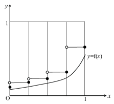
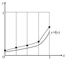
Figure 6. Overapproximation by a step-function (left) and a stepwise linear function (right)

The following lemma ensures that the inequality (2) is indeed a sufficient condition for $\gamma(\vec{r})$ to be an upper-bound on $\mathbf{lfp}(\mathcal{F})$. Note that both step functions and stepwise linear functions satisfy the assumption of the lemma below.

Lemma 5.3.

Suppose that the concretization function $\gamma$ is monotonic, and that $\vec{r}\geq\alpha(f)$ implies $\gamma(\vec{r})\geq f$ for every pointwise convex $f$. Then, any abstract pre-fixpoint of $\mathcal{F}$ is an upper bound of $\mathbf{lfp}(\mathcal{F})$.

Proof 5.4.

First, we show that $\gamma(\widehat{\mathcal{F}}^{m}(\bot))\geq\mathcal{F}^{m}(\bot)$ holds for every $m$, by induction on $m$. The base case $m=0$ is trivial, since $\mathcal{F}^{0}(\bot)=\bot$. If $m>0$, then we have

$$\begin{array}[]{l}\widehat{\mathcal{F}}^{m}(\bot)=\alpha(\mathcal{F}(\gamma(\widehat{\mathcal{F}}^{m-1}(\bot))))\geq\alpha(\mathcal{F}(\mathcal{F}^{m-1}(\bot)))=\alpha(\mathcal{F}^{m}(\bot)).\end{array}$$

Since, by hypothesis, $\vec{r}\geq\alpha(\mathcal{F}^{m}(\bot))$ implies that $\gamma(\vec{r})\geq\mathcal{F}^{m}(\bot)$ (since $\mathcal{F}^{m}(\bot)$ is pointwise convex), we can conclude that $\gamma(\widehat{\mathcal{F}}^{m}(\bot))\geq\mathcal{F}^{m}(\bot)$. Now, suppose $\vec{r}$ is an abstract pre-fixpoint of $\mathcal{F}$. Then $\gamma(\vec{r})\geq\gamma(\widehat{\mathcal{F}}^{m}(\vec{r}))\geq\gamma(\widehat{\mathcal{F}}^{m}(\bot))\geq\mathcal{F}^{m}(\bot)$, and as $\mathcal{F}$ is $\omega$-continuous, we have $\gamma(\vec{r})\geq\sup_{\_}{m\in\omega}\mathcal{F}^{m}(\bot)=\mathbf{lpf}(\mathcal{F})$ as required.

Below we consider the combination of (b) and (d). Figure 7 shows a pseudo code for computing an upper-bound of $f(c)$ for the least solution $f$ of $f(x)=e$ and $c\in[0,1]$. In the figure, $\alpha_{\_}h(x)=\frac{\lceil{mx}\rceil}{m}$. The algorithm terminates under the assumptions that (i) $e$ consists of non-negative constants, $x$, $+$, $\cdot$, and applications of $f$, and (ii) every subexpression of $e$ evaluates to a value in $[0,1]$ (if $x\in[0,1]$ and $f\in[0,1]\to[0,1]$), which are satisfied by the fixpoint equations obtained from a PHORS (recall Section 5.1).

main($e$, $c$){
  $r$ := $[0,\ldots,0]$;  $r^{\prime}$ := $[1,\ldots,1]$ (* dummy *);
  while not($r$=$r^{\prime}$) do {
    $r^{\prime}$ := $r$; (* copy the contents of array $r$ to $r^{\prime}$ *)
    for each $i\in\{0,\ldots,n\}$ do $r^{\prime}[i]$ := $\alpha_h$(eval($e$, $\{f\mapsto r,x\mapsto\frac{i}{n}\}$))};
  return apply($r$, $c$); }
apply($r$, $c$) { (* apply the function represented by array $r$ to $c$ *)
  $i$ := $\lfloor{nc}\rfloor$; (* $\frac{i}{n}\leq c<\frac{i+1}{n}$ *)
  return $(i+1-nc)r[i]+(nc-i)r[i+1]$; }
eval($e$, $\rho$){
  match $e$ with
     $x$ $\to$ return $\rho(x)$ |  $c$ $\to$ return $c$
   | $f(e^{\prime})$ $\to$ return apply($\rho(f)$, eval($e^{\prime}$, $\rho$))
   | $e_1+e_2$ $\to$ return eval($e_1$,$\rho$)+eval($e_2$,$\rho$)
   | $e_1\cdot{}e_2$ $\to$ return eval($e_1$,$\rho$)$\cdot$eval($e_2$,$\rho$) }

Figure 7. Pseudo code for computing an upper-bound of $f(c)$ where $f(x)=e$ (unary function case)

Example 5.5.

Consider $f(x)=\frac{1}{4}x+\frac{3}{4}f(f(x))$ and let $n=2$ and $m=4$. The value $r^{(j)}$ of $r$ after the $j$-th iteration is given by:

$$r^{(0)}=[0,0,0];\qquad r^{(1)}=[0,0.25,0.25];\qquad r^{(2)}=[0,0.25,0.5];\qquad r^{(3)}=[0,0.25,0.5].$$

Thus, the upper-bound obtained for $f(1)$ is $0.5$. The exact value of $f(1)=\frac{1}{3}$. A more precise upper-bound is obtained by increasing the values of $n$ and $m$. For example, if $n=16$ and $m=256$, the upper-bound (obtained by running the tool reported in a later section) is $0.3398\cdots$. ∎

5.2.2. Computing an upper-bound for a binary function

We now consider a fixpoint equation of the form $f(x_{\_}1,x_{\_}2)=e$, where $x_{\_}1$ and $x_{\_}2$ are such that $0\leq x_{\_}1,x_{\_}2$, and $x_{\_}1+x_{\_}2\leq 1$. Such an equation is obtained from an order-2 PHORS by using the fixpoint characterization in the previous section. A new difficulty compared with the unary case is that $f(x_{\_}1,x_{\_}2)$ may take a value outside $[0,1]$, or may even be undefined for $(x_{\_}1,x_{\_}2)\in[0,1]\times[0,1]$ such that $x_{\_}1+x_{\_}2>1$. Figure 8 shows how we discretize the domain of $f$. The grey-colored and red-colored areas show the valid domain of $f$, for which we wish to approximate $f(x_{\_}1,x_{\_}2)$ using the values at discrete points. An upper-bound of the value of $f$ at a point $(x_{\_}1,x_{\_}2)$ in the grey area can be obtained by (pointwise) linear interpolations from (upper-bounds of) the values at the surrounding four points, i.e., $(\frac{i_{\_}1}{n},\frac{i_{\_}2}{n}),(\frac{i_{\_}1}{n},\frac{i_{\_}2+1}{n}),(\frac{i_{\_}1+1}{n},\frac{i_{\_}2}{n}),(\frac{i_{\_}1+1}{n},\frac{i_{\_}2+1}{n})$ where $x_{\_}1\in[\frac{i_{\_}1}{n},\frac{i_{\_}1+1}{n}]$ and $x_{\_}2\in[\frac{i_{\_}2}{n},\frac{i_{\_}2+1}{n}]$, as follows.

$$\begin{array}[]{l}\hat{f}(x_{\_}1,x_{\_}2)\\ =(i_{\_}2+1-nx_{\_}2)\hat{f}(x_{\_}1,\frac{i_{\_}2}{n})+(nx_{\_}2-i_{\_}2)\hat{f}(x_{\_}1,\frac{i_{\_}2+1}{n})\\ =(i_{\_}2+1-nx_{\_}2)(i_{\_}1+1-nx_{\_}1)\hat{f}(\frac{i_{\_}1}{n},\frac{i_{\_}2}{n})\\ \qquad+(i_{\_}2+1-nx_{\_}2)(nx_{\_}1-i_{\_}1)\hat{f}(\frac{i_{\_}1+1}{n},\frac{i_{\_}2}{n})\\ \qquad+(nx_{\_}2-i_{\_}2)(i_{\_}1+1-nx_{\_}1)\hat{f}(\frac{i_{\_}1}{n},\frac{i_{\_}2+1}{n})\\ \qquad+(nx_{\_}2-i_{\_}2)(nx_{\_}1-i_{\_}1)\hat{f}(\frac{i_{\_}1+1}{n},\frac{i_{\_}2+1}{n}).\end{array}$$

Note that $\hat{f}(x,y)\geq f(x,y)$ at the four points imply that $\hat{f}(x_{\_}1,x_{\_}2)\geq f(x_{\_}1,x_{\_}2)$, because $f(x,y)$ is convex on each of $x$ and $y$ (recall Section 5.1).

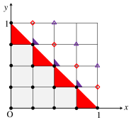
Figure 8. Discretization in the case of a binary function $f(x,y)$, whose domain is $\{(x,y)\mid 0\leq x,0\leq y,x+y\leq 1\}$ (i.e., the grey and red areas). Outside the domain, the value of $f(x,y)$ may not belong to $[0,1]$, or may be even undefined. The value at a point in the grey area can be estimated by using those at discrete points $\bullet$. To estimate the value at a point in the red area, we also need the value of $f(x,y)$ at a point marked by ${\color[rgb]{1,0,0}\Diamond}$.

A difficulty is that to estimate the value of $f$ at a point in the red area, we need the value at a red point $\Diamond$, but the value of $f$ at the red point may be greater than 1 or even $\infty$, being outside $f$’s domain. To this end, we discretize the codomain of $f$ to $\{0,\frac{1}{m},\ldots,\frac{mh-1}{m},h,\infty\}$ (instead of $\{0,\frac{1}{m},\ldots,\frac{m-1}{m},1\}$) for some $h\geq 1$. Any value greater than $h$ is approximated to $\infty$. The value at a point in the red area is then approximated in the same way as for the case of a point in the grey area, except that if $\hat{f}(\frac{i_{\_}1+1}{m},\frac{i_{\_}2+1}{m})=\infty$, then $\hat{f}(x_{\_}1,x_{\_}2)=1$.

A further complication arises when the equation contains function compositions, as in $f(x_{\_}1,x_{\_}2)=E[f(f(x_{\_}1,x_{\_}2),x_{\_}2)]$ where $E$ denotes some context. In this case, the point $(\hat{f}(x_{\_}1,x_{\_}2),x_{\_}2)$ may even be outside the area surrounded by $\Diamond$ and $\bullet$-points either if $(x_{\_}1,x_{\_}2)$ is a $\Diamond$-point or if $(x_{\_}1,x_{\_}2)$ is a $\bullet$-point but $\hat{f}(x_{\_}1,x_{\_}2)+x_{\_}2$ is too large due to an overapproximation. In such a case, $(\hat{f}(x_{\_}1,x_{\_}2),x_{\_}2)$ belongs to the purple area (lower left triangles) in the figure. To this end, we also compute (upper-bounds of) the values at points marked by $\triangle$ and use them to estimate the value at a point in the purple area. If the point $(\hat{f}(x_{\_}1,x_{\_}2),x_{\_}2)$ is even outside the area surrounded by $\bullet$, $\Diamond$, or $\triangle$, then we use $\infty$ as an upper-bound of $f(f(x_{\_}1,x_{\_}2),x_{\_}2)$ if $(x_{\_}1,x_{\_}2)$ is a $\Diamond$-, or $\triangle$-point, and $1$ if $(x_{\_}1,x_{\_}2)$ is a $\bullet$-point.

Except the above differences, the overall algorithm is similar to the unary case in Figure 7, and essentially the same soundness argument as Lemma 5.3 applies.

Example 5.6.

Consider $f(x_{\_}1,x_{\_}2)=x_{\_}1+x_{\_}2(f(x_{\_}1,x_{\_}2))^{2}$, and let $n=m=2$. The value of $r=\left(\begin{array}[]{ccc}r_{\_}{0,2}&r_{\_}{1,2}&r_{\_}{2,2}\\ r_{\_}{0,1}&r_{\_}{1,1}&r_{\_}{2,1}\\ r_{\_}{0,0}&r_{\_}{1,0}&r_{\_}{2,0}\end{array}\right)$, where $r_{\_}{i,j}$ is an upper-bound of the value of $f(\frac{i}{2},\frac{j}{2})$, changes as follows.

$$\begin{array}[]{l}\left(\begin{array}[]{ccc}0&0&0\\ 0&0&0\\ 0&0&0\end{array}\right)\longrightarrow\left(\begin{array}[]{ccc}0&0.5&1\\ 0&0.5&1\\ 0&0.5&1\end{array}\right)\longrightarrow\left(\begin{array}[]{ccc}0&1&\infty\\ 0&1&\infty\\ 0&0.5&1\end{array}\right)\longrightarrow\left(\begin{array}[]{ccc}0&\infty&\infty\\ 0&1&\infty\\ 0&0.5&1\end{array}\right)\end{array}$$

Thus, for example, $f(0,0.5)$ and $f(0.3,0.3)$ are overapproximated respectively by $0$ and $0.36\hat{f}(0.5,0.5)+0.24\hat{f}(0.5,0)+0.24\hat{f}(0,0.5)+0.16\hat{f}(0,0)=0.48$. The exact values for $f(0,0)$ and $f(0.3,0.3)$ are $0$ and $\frac{1}{3}$; so the upper-bound for $f(0.3,0.3)$ is sound but imprecise. By choosing $n=16$ and $m=256$, we obtain $0.3359\cdots$ as an upper-bound of $f(0.3,0.3)$.

This is an example where the values of $f$ at red points in Figure 8 are $\infty$. The exact value of $f(x_{\_}1,x_{\_}2)$ for general $x_{\_}1$ and $x_{\_}2$ is given by:

$$f(x_{\_}1,x_{\_}2)=\left\{\begin{array}[]{ll}x_{\_}1&\mbox{if $x_{\_}2=0$}\\ \frac{1-\sqrt{1-4x_{\_}1x_{\_}2}}{2x_{\_}2}&\mbox{if $x_{\_}1>0$}\end{array}\right.$$

Thus, $f(0.5,0.5)=1$, but $f(x_{\_}1,x_{\_}2)$ is undefined whenever $x_{\_}1x_{\_}2>0.25$; in particular $f(0.5,1)$ and $f(1,0.5)$ (the values of red points in Figure 8 for the case $n=2$) are undefined. ∎

5.2.3. Computing an Upper-Bound: General Case

The binary case discussed above can be easily extended to handle the general case, where the goal is to estimate the value of $f_{\_}1(c_{\_}1,\ldots,c_{\_}{\ell_{\_}1})$ for the least solution of the fixpoint equations:

$$f_{\_}1(x_{\_}1,\ldots,x_{\_}{\ell_{\_}1})=e_{\_}1\qquad\cdots\qquad f_{\_}k(x_{\_}1,\ldots,x_{\_}{\ell_{\_}k})=e_{\_}k.$$

Here, the formal arguments $x_{\_}1,\ldots,x_{\_}{\ell_{\_}i}$ of each function $f_{\_}i$ are partitioned into several groups $(x_{\_}1,\ldots,x_{\_}{d_{\_}{i,1}}),(x_{\_}{d_{\_}{i,1}+1},\ldots,x_{\_}{d_{\_}{i,2}}),\ldots,(x_{\_}{d_{\_}{g_{\_}{i}-1}+1},\ldots,x_{\_}{\ell_{\_}i})$, so that the sum of the values of the variables in each group ranges over $[0,1]$. Following the binary case, we discretize the domain so that each variable ranges over $\{0,\frac{1}{n},\ldots,\frac{n-1}{n},1\}$, where the variables in each group $(x_{\_}{d_{\_}{i,j-1}+1},\ldots,x_{\_}{d_{\_}{i,j}})$ are constrained by $x_{\_}{d_{\_}{i,j-1}+1}+\cdots+x_{\_}{d_{\_}{i,j}}\leq\frac{n+2}{n}$. Note that we choose $\frac{n+2}{n}$ instead of $1$ as the upper-bound of the sum, to include the points $\Diamond$ and $\triangle$ in Figure 8. We write $D_{\_}i$ for the discretized domain of function $f_{\_}i$, and $D_{\_}i^{\prime}$ for the subset of $D_{\_}i$ where the variables in each group are constrained by $x_{\_}{d_{\_}{i,j-1}+1}+\cdots+x_{\_}{d_{\_}{i,j}}\leq 1$; note that $f_{\_}i(x_{\_}1,\ldots,x_{\_}{\ell_{\_}i})\in[0,1]$ for $(x_{\_}1,\ldots,x_{\_}{\ell_{\_}i})\in D_{\_}i^{\prime}$, but $f_{\_}i(x_{\_}1,\ldots,x_{\_}{\ell_{\_}i})$ may be greater than $1$ or undefined for $(x_{\_}1,\ldots,x_{\_}{\ell_{\_}i})\in D_{\_}i\setminus D_{\_}i^{\prime}$. We also write $\overline{D_{\_}i}$ for the set $\{(x_{\_}1,\ldots,x_{\_}{\ell_{\_}i})\mid(\lceil{nx_{\_}1}\rceil/n,\ldots,\lceil{nx_{\_}{\ell_{\_}i}}\rceil/n)\in D_{\_}i\}$ (i.e., the set of points for which the value of $f_{\_}i$ can be approximated by using values at points in $D_{\_}i$).

The pseudo code for computing an upper-bound of $f_{\_}1(c_{\_}1,\ldots,c_{\_}{\ell_{\_}1})$ is given in Figure 9. On the 9th line (“$\texttt{if }\vec{v}\in D_{\_}i^{\prime}\texttt{ then ...}$”), we also make use of the constraint that $\Sigma_{\_}{f^{\prime}\in\mathtt{fgrp}(f_{\_}i)}f^{\prime}(\widetilde{v})$ ranges over $[0,1]$ if $\widetilde{v}$ belongs to the valid domain $D_{\_}i^{\prime}$ (recall the 3rd property in Section 5.1). We assume that the procedure $\texttt{lb}(f^{\prime},\widetilde{v})$ returns a sound lower-bound of $f^{\prime}(\widetilde{v})$, e.g., by using Kleene iteration. See Remark 5.7 to understand the need for this additional twist.

main($e_1,\ldots,e_k$, $\vec{c}$){
  $\rho$ := $[f_1\mapsto[\vec{0}],\ldots,f_k\mapsto[\vec{0}]]$;
      (* $\rho(f_i)$ is an array indexed by each element of $D_i$ *)
  $\rho^{\prime}$ := $[f_1\mapsto[\vec{1}],\ldots,f_k\mapsto[\vec{1}]]$; (* dummy *)
  while not($\rho$=$\rho^{\prime}$) do {
    $\rho^{\prime}$ := $\rho$; (* copy the contents *)
    for each $i\in\{0,\ldots,k\}$ do
       for each $\vec{v}\in{}D_i$ do
          let r = eval($e_i$, $\rho\{\vec{x}\mapsto\vec{v}\}$, $\vec{v}\stackrel{{\scriptstyle?}}{{\in}}D^{\prime}_i$) in
            if $\vec{v}\in D^{\prime}_i$ then $\rho^{\prime}(f_i)[\vec{v}]$ := $\alpha_h$(min(r, $1-\Sigma_{f^{\prime}\in\mathtt{fgrp}(f_i)\setminus\{f\}}$ lb($f^{\prime}$, $\vec{v}$)))
            else $\rho^{\prime}(f_i)[\vec{v}]$ := $\alpha_h$(r);
  return apply($\rho(f_1)$, $\vec{c}$); }

eval($e$, $\rho$, $b$){
 (* $b$ represents whether we are computing the value of $f_i$ in the valid
    domain; in that case, the value of $e$ should range over $[0,1]$. *)
  let $r$ =
    match $e$ with
       $x$ $\to$ $\rho(x)$ | $c$ $\to$ $c$
     | $f_i(\vec{e^{\prime}})$ $\to$ let $\vec{v}$ = eval($\vec{e^{\prime}}$,$\rho$,$b$) in
                 if $\vec{v}\not\in\overline{D_i}$ then $\infty$ else apply($\rho(f_i)$, $\vec{v}$)
     | $e_1+e_2$ $\to$ eval($e_1$, $\rho$, $b$)+eval($e_2$, $\rho$, $b$)
     | $e_1\cdot{}e_2$ $\to$ eval($e_1$, $\rho$, $b$)$\cdot$eval($e_2$, $\rho$, $b$)
  in if $b$ then return min($r$,1) else return $r$ }

Figure 9. Pseudo code for computing an upper-bound for the general case

The function $\alpha_{\_}h$ takes a real value (or $\infty$) $x$, and returns the least element in $\{0,\frac{1}{n},\ldots,\frac{mh-1}{m},h,\infty\}$ that is no less than $x$. The function apply in the figure takes the current approximations of values of $f_{\_}i$ at the points $D_{\_}i$ and the arguments $\vec{v}\in\overline{D_{\_}i}$, and returns an approximation of $f_{\_}i(\vec{v})$. It is given by $\hat{f}(\vec{v})$, where:

$$\begin{array}[]{l}\hat{f_{\_}i}(x_{\_}1,\ldots,x_{\_}{\ell_{\_}i})=\sum_{\_}{b_{\_}1,\ldots,b_{\_}{\ell_{\_}i}\in\{0,1\}}p_{\_}1^{b_{\_}1}(1-p_{\_}1)^{1-b_{\_}1}\cdots p_{\_}{\ell_{\_}i}^{b_{\_}{\ell_{\_}i}}(1-p_{\_}{\ell_{\_}i})^{1-b_{\_}{\ell_{\_}i}}\hat{f_{\_}i}\left(\frac{i_{\_}1+b_{\_}1}{n},\ldots,\frac{i_{\_}{\ell_{\_}i}+b_{\_}{\ell_{\_}i}}{n}\right)\end{array}$$

Here, $i_{\_}j=\lfloor{nx_{\_}j}\rfloor$, $p_{\_}j=nx-i_{\_}j$, and $\hat{f_{\_}i}(\frac{i_{\_}1+b_{\_}1}{n},\ldots,\frac{i_{\_}m+b_{\_}m}{n})$ is the current approximation of the value of $f_{\_}i$ at $(\frac{i_{\_}1+b_{\_}1}{n},\ldots,\frac{i_{\_}m+b_{\_}m}{n})\in D_{\_}i$. The function $\hat{f}$ above is obtained by applying linear interpolations coordinate-wise.

Remark 5.7.

To see the motivation for the 9th line in Figure 9, consider the following fixpoint equations:

$$S =f_{\_}1()$$

$$f_{\_}1() =0.5\cdot(f_{\_}1()\cdot f_{\_}1()+f_{\_}2()\cdot f_{\_}2())$$

$$f_{\_}2() =0.5+f_{\_}1()\cdot f_{\_}2().$$

They are obtained from the following order-1 PHORS $\mathcal{G}_{\_}{\mathtt{treeeven}}$:

$$S\,z =F\,z\,\Omega$$

$$F\;x_{\_}1\;x_{\_}2 =x_{\_}2\,\oplus_{p}\,F\;(F\;x_{\_}1\;x_{\_}2)\;(F\;x_{\_}2\;x_{\_}1),$$

where $p=0.5$, and $f_{\_}1()$ ($f_{\_}2()$, resp.) represents the probability that $x_{\_}1$ ($x_{\_}2$, resp.) is used by $F$. This PHORS is actually a variation of $\mathcal{G}_{\_}6$ from Example 2.9 (with manual optimization), whose termination probability represents the probability that a program that randomly generates binary trees (instead of lists, unlike in the case of Example 2.9) contains an even number of leaves. Since the events that $F$ uses the first and second arguments are mutually exclusive, we have the constraint $f_{\_}1()+f_{\_}2()\leq 1$. The exact solution for the equations above is $f_{\_}1()=1-\frac{1}{\sqrt{2}}$ and $f_{\_}2()=\frac{1}{\sqrt{2}}$. Since their lower-bounds can be computed with arbitrary precision, thanks to the part $1-\Sigma_{\_}{f^{\prime}\in\mathtt{fgrp}(f_{\_}i)\setminus\{f\}}$ lb($f^{\prime}$, $\vec{v}$) of the 9th line of Figure 9, we can also compute upper-bounds with arbitrary precision (as upper-bounds of $f_{\_}1()$ and $f_{\_}2()$ are respectively provided by $1-\texttt{lb}(f_{\_}2,())$ and $1-\texttt{lb}(f_{\_}1,())$).

If the then-clause were the same as the else-clause on the 10th line, then we would not get a precise upper-bound for the following reason. When the main loop in Figure 9 stops, upper-bounds $\overline{f}_{\_}1()$ and $\overline{f}_{\_}2()$ must either have reached the maximal value $1$, or satisfy:

$$\begin{array}[]{l}\overline{f}_{\_}1()\geq 0.5\cdot(\overline{f}_{\_}1()\cdot\overline{f}_{\_}1()+\overline{f}_{\_}2()\cdot\overline{f}_{\_}2())\\ \overline{f}_{\_}2()\geq 0.5+\overline{f}_{\_}1()\cdot\overline{f}_{\_}2().\end{array}$$

These conditions imply that:

$$\overline{f}_{\_}1()+\overline{f}_{\_}2()\geq 0.5\cdot(\overline{f}_{\_}1()\cdot\overline{f}_{\_}1()+\overline{f}_{\_}2()\cdot\overline{f}_{\_}2())+0.5+\overline{f}_{\_}1()\cdot\overline{f}_{\_}2(),$$

i.e.,

$$0\geq(\overline{f}_{\_}1()+\overline{f}_{\_}2()-1)^{2},$$

which is equivalent to $\overline{f}_{\_}1()+\overline{f}_{\_}2()=1$. Thus, unless the co-domain of $\alpha_{\_}h$ contains the exact values $1-\frac{1}{\sqrt{2}}$ and $\frac{1}{\sqrt{2}}$, the main loop would only return the imprecise upper-bound $\overline{f}_{\_}1()=\overline{f}_{\_}2()=1$. ∎

5.3. Order-$n$ Case

We now briefly discuss how to extend the method discussed above to obtain a sound (but incomplete) method for overapproximating the termination probability of PHORS of order greater than 2. Recall that by the fixpoint characterization given in Section 4.3, it suffices to overapproximate the least solution of equations of the form $\vec{f}={\mathcal{F}}(\vec{f})$ where $\vec{f}$ is a tuple of order-($n-1$) functions on reals.

The abstract interpretation framework [Cou97] provides a sound but incomplete methodology: the reason why we decided to slightly divert from it in Section 5.2 is that this allows us to use piecewise linear functions, which are more precise. We first recall a basic principle of abstract interpretation. Let $(C,\sqsubseteq_{\_}C,\bot_{\_}C)$ and $(A,\sqsubseteq_{\_}A,\bot_{\_}A)$ be $\omega$-cpos. Suppose that $\alpha:(C,\sqsubseteq_{\_}C)\to(A,\sqsubseteq_{\_}A)$ and $\gamma:(A,\sqsubseteq_{\_}A)\to(C,\sqsubseteq_{\_}C)$ are continuous (hence also monotonic) such that $\alpha(\gamma(a))=a$ for every $a\in A$, and $c\sqsubseteq_{\_}C\gamma(\alpha(c))$ for every $c\in C$. Suppose also that $\mathcal{F}$ is a continuous function from $(C,\sqsubseteq_{\_}C,\bot_{\_}C)$ to $(C,\sqsubseteq_{\_}C,\bot_{\_}C)$. Let $\widehat{\mathcal{F}}:(A,\sqsubseteq_{\_}A,\bot_{\_}A)\to(A,{\sqsubseteq_{\_}A},\bot_{\_}A)$ be $\lambda x\in A.\alpha(\mathcal{F}(\gamma(x)))$, which is an “abstract version” of $\mathcal{F}$. Note that $\widehat{\mathcal{F}}$ is also continuous. Then, we have:

Proposition 5.8.

$\mathbf{lfp}(\mathcal{F})\sqsubseteq_{\_}C\gamma(\mathbf{lfp}(\widehat{\mathcal{F}}))$.

This result is standard (see, e.g., [Cou97], Proposition 18) but we provide a proof for the convenience of the reader.

Proof 5.9 (Proof of Proposition 5.8).

By the monotonicity of $\mathcal{F}$ and $\widehat{\mathcal{F}}$, we have: $\bot_{\_}C\sqsubseteq_{\_}C\mathcal{F}(\bot_{\_}C)\sqsubseteq_{\_}C\mathcal{F}^{2}(\bot_{\_}C)\sqsubseteq_{\_}C\cdots$ and $\bot_{\_}A\sqsubseteq_{\_}A\widehat{\mathcal{F}}(\bot_{\_}A)\sqsubseteq_{\_}A{\widehat{\mathcal{F}}}^{2}(\bot_{\_}A)\sqsubseteq_{\_}A\cdots$; hence both ${\bigsqcup_{\_}C}\{\mathcal{F}^{i}(\bot_{\_}C)\mid{i\in\omega}\}$ and ${\bigsqcup_{\_}A}\{{\widehat{\mathcal{F}}}^{i}(\bot_{\_}A)\mid i\in\omega\}$ exist, and by the $\omega$-continuity of $\mathcal{F}$ and $\widehat{\mathcal{F}}$, they are the least fixpoints of $\mathcal{F}$ and $\widehat{\mathcal{F}}$ respectively. Therefore, it suffices to show that $\mathcal{F}^{i}(\bot_{\_}C)\sqsubseteq_{\_}C\gamma({\widehat{\mathcal{F}}}^{i}(\bot_{\_}C))$. The proof proceeds by induction on $i$. The base case $i=0$ is trivial. If $i>0$, we have:

$$\gamma({\widehat{\mathcal{F}}}^{i}(\bot_{\_}C)) =\gamma(\alpha(\mathcal{F}(\gamma({\widehat{\mathcal{F}}}^{i-1}(\bot_{\_}C))))) \widehat{\mathcal{F}}$$ (by the definition of )

$$\sqsupseteq_{\_}C\mathcal{F}(\gamma({\widehat{\mathcal{F}}}^{i-1}(\bot_{\_}C))) \gamma(\alpha(x))\sqsupseteq_{\_}Cx$$ (by )

$$\sqsupseteq_{\_}C\mathcal{F}(\mathcal{F}^{i-1}(\bot_{\_}C))$$ (by induction hypothesis)

$$=\mathcal{F}^{i}(\bot_{\_}C).$$

By the proposition above, to overapproximate the least fixpoint of $\mathcal{F}$, it suffices to find an appropriate abstract domain $(A,\sqsubseteq_{\_}A,\bot_{\_}A)$ and $\alpha,\gamma$ that satisfy the conditions above, so that the least fixpoint of $\widehat{\mathcal{F}}$ is easily computable. In the case of overapproximation of the termination probability of order-$n$ PHORS, we need to set up an abstract domain $(A,\sqsubseteq_{\_}A,\bot_{\_}A)$ for a tuple of order-($n-1$) functions on reals. A simple solution (that is probably too naive in practice) is to use the abstract domain consisting of higher-order step functions, inductively defined by:

$$A^{\mathtt{R}} =\{\frac{0}{m},\frac{1}{m},\ldots,\frac{m-1}{m},\frac{m}{m},\infty\}$$

$$\sqsubseteq_{\_}{A^{\mathtt{R}}} =\{(\frac{i}{m},\frac{j}{m})\mid 0\leq i\leq j\leq m\}\cup\{(\frac{i}{m},\infty)\mid 0\leq i\leq m\}$$

$$\alpha^{\mathtt{R}}(x) =\left\{\begin{array}[]{ll}\frac{i}{m}&\mbox{if $\frac{i-1}{m}\leq x\leq\frac{i}{m}$}\\ \infty&\mbox{if $x>1$}\end{array}\right.$$

$$\gamma^{\mathtt{R}}(x) =x$$

$$A^{\tau_{\_}1\to\tau_{\_}2} =\{f\in A^{\tau_{\_}1}\to A^{\tau_{\_}2}\mid\mbox{$f$ is monotonic}\}$$

$$\sqsubseteq_{\_}{A^{\tau_{\_}1\to\tau_{\_}2}} =\{(f_{\_}1,f_{\_}2)\in A^{\tau_{\_}1\to\tau_{\_}2}\times A^{\tau_{\_}1\to\tau_{\_}2}\mid\forall x\in A^{\tau_{\_}1\to\tau_{\_}2}.f_{\_}1\,x\sqsubseteq_{\_}{A^{\tau_{\_}2}}f_{\_}2\,x\}$$

$$\alpha^{\tau_{\_}1\to\tau_{\_}2}(f) =\{(y,\alpha^{\tau_{\_}2}(f(\gamma^{\tau_{\_}1}(y))))\mid y\in A^{\tau_{\_}1}\}$$

$$\gamma^{\tau_{\_}1\to\tau_{\_}2}(f^{\prime}) =\{(x,\gamma^{\tau_{\_}2}(f^{\prime}(\alpha^{\tau_{\_}1}(x))))\mid x\in C^{\tau_{\_}1}\}.$$

Here, the concrete domain $C^{\tau}$ denotes $\llbracket{\tau}\rrbracket$ in Section 4.1. Then, $\alpha^{\tau}$ and $\beta^{\tau}$ satisfy the required conditions ($\alpha(\gamma(a))=a$ and $c\sqsubseteq_{\_}C\gamma(\alpha(c))$). Since $A^{\tau}$ is finite, we can effectively compute $\mathbf{lfp}(\widehat{\mathcal{F}})$.

We note, however, that the above approach has the following shortcomings. First, although $A^{\tau}$ is finite, its size is too large: $k$-fold exponential for order-$k$ type $\tau$. As in the case of non-probabilistic HORS model checking [Kob09a, BK13, RNO14], therefore, we need a practical algorithm that avoids eager enumeration of abstract elements. Second, due to the use of step functions, the obtained upper-bound will be too imprecise. To see why step functions suffer from the incompleteness, consider the equations: $s=f(\frac{1}{2})$ and $f(x)=\frac{1}{2}x+f(\frac{1}{2}x)$. The exact least solution is $s=\frac{1}{2}$ and $f(x)=x$. With step functions (where $\frac{1}{n}$ is the size of each interval), however, the abstract value $\hat{f}(\frac{1}{n})$ must be no less than $\frac{1}{2}\frac{1}{n}+f(\frac{1}{2}\cdot\frac{1}{n})$, but $f(\frac{1}{2}\cdot\frac{1}{n})$ is overapproximated as $\hat{f}(\frac{1}{n})$ (because $\frac{1}{2n}$ belongs to the interval $(0,\frac{1}{n}]$). Therefore, $\hat{f}(\frac{1}{n})$ should be no less than $\frac{1}{2n}+\hat{f}(\frac{1}{n})$, which is impossible. Thus, the computation diverges and $1$ is obtained as an obvious upper bound.

The step functions only use monotonicity of the least solution of fixpoint equations. As in the use of stepwise multilinear functions in the case of order-1 equations (for order-2 PHORS), exploiting an additional property like convexity would be important for obtaining a more precise method; this is left for future work.

6. Experiments

We have implemented a prototype tool to compute lower/upper bounds of the least solution of order-1 fixpoint equations (that are supposed to have been obtained from order-2 or order-1 PHORS by using the translations in Section 4 modulo some simplifications; we have not yet implemented the translators from PHORS to fixpoint equations, which is easy but tedious). The computation of a lower bound is based on naive Kleene iterations, and that of an upper-bound is based on the method discussed in Section 5.2. The tool uses floating point arithmetic, and ignores rounding errors.

We have tested the tool on several small but tricky examples. The experimental results are summarized in Table 2. The column “equations” lists the names of systems of equations. The column “#iter” shows the number of Kleene iterations used for computing a lower-bound. The columns “#dom” and “#codom” show the numbers of partitions of the interval $[0,1]$ for the domain and codomain of a function respectively. The default values for them were set to 12, 16, and 512, respectively in the experiment; they were, however, adjusted for some of the equations. The columns “l.b.” and “u.b.” are lower/upper bounds computed by the tool. The lower (upper, resp.) bounds shown in the table have been obtained by rounding down (up, resp.) the outputs of the tool to 3-decimal places. The column “step” shows the upper-bounds obtained by using step functions instead of piecewise linear functions; this column has been prepared to confirm the advantage of piecewise linear functions over step functions. The column “exact” shows the exact value of the least solution when we know it. The column “time” shows the total time for computing both lower and upper bounds (excluding the time for “step”).

Table 2. Experimental results (times are in seconds).

equations	#iter	#dom	#codom	l.b.	u.b.	step	exact	time
Ex2.3-1	12	16	512	0.333	0.336	1.0	$\frac{1}{3}$	0.010
Ex2.3-0	12	16	512	0.333	0.334	0.334	$\frac{1}{3}$	0.008
Ex2.3-v1	12	16	512	0.312	0.315	0.365	-	0.005
Ex2.3-v2	12	16	512	0.262	0.266	0.321	-	0.022
Ex2.3-v3	12	16	512	0.263	0.266	0.309	-	0.01
Ex2.4	12	16	512	0.320	0.323	0.329	-	0.011
Double	12	16	512	0.649	0.653	1.0	-	0.010
Listgen	15	16	512	0.999	1.0	1.0	1.0	0.009
Treegen	15	64	4096	0.618	0.619	1.0	$\frac{\sqrt{5}-1}{2}$	0.471
Treegenp	12	16	512	1.0	1.0	1.0	1.0	0.011
ListEven	12	32	1024	0.666	0.667	0.667	$\frac{2}{3}$	0.009
ListEven2	12	16	512	0.749	0.75	0.75	$\frac{3}{4}$	0.013
Determinize	12	16	512	0.993	1.0	1.0	1.0	9.64
TreeEven(0.5)	15	64	4096	0.286	0.299	0.300	$1-\frac{1}{\sqrt{2}}$	0.050
TreeEven(0.49)	15	64	4096	0.276	0.280	0.280	0.2774$\cdots$	0.052
TreeEven(0.51)	15	64	4096	0.287	0.290	0.290	0.2887$\cdots$	0.055
Ex5.4(0,0)	12	16	512	0.0	0.0	0.0	0	0.008
Ex5.4(0.3,0.3)	12	16	512	0.333	0.336	0.35	$\frac{1}{3}$	0.007
Ex5.4(0.5,0.5)	10000	16	512	0.999	1.0	1.0	1	0.010
Discont(0,1)	12	16	512	0.0	0.0	0.0	0	0.006
Discont(0.01,0.99)	1000	16	512	0.999	1.0	1.0	1	0.006
Incomp	10000	16	512	0.299	1.0	1.0	0.3	0.003
Incomp	10000	10	100	0.299	0.3	0.3	0.3	0.003
Incomp2	12	16	512	0.249	1.0	1.0	0.25	0.003
Incomp2	12	256	65536	0.249	1.0	1.0	0.25	2.87

The equations “Ex2.3-1” and “Ex2.3-0” are order-1 and order-0 equations obtained from the PHORS in Example 2.1 (see also Examples 4.4 and 4.6) by using the translations in Sections 4.2 and 4.3 respectively; specifically, “Ex2.3-1” consists of $s=f(1)$ and $f(x)=0.25x+0.75f(f(x))$. The equations “Ex2.3-v1”, “Ex2.3-v2”, and “Ex2.3-v3” are variations of them, where the equation on $f$ is replaced by $f(x)=0.25x+0.75f(f(x^{2}))$, $f(x)=0.25x+0.75f(f(f(x^{2})))$, and $f(x)=0.25x+0.75(f(x))^{2}$, respectively. “Ex2.4” is the equations obtained from the order-2 PHORS in Example 2.2 (see also Example 4.7). The equations “Double” are those obtained from the following order-2 PHORS:

$$S\ =\ F\,H$$

$$H\,x\,y =x\,\oplus_{\frac{1}{2}}\,y$$

$$F\,g =g\,\mathtt{e}\,(F(D\,g))$$

$$D\,g\,x\,y =g\,(g\,x\,y)\,y,$$

with manual simplifications. The equations “Listgen”, “Treegen”, and “Treegenp” are from Example 2.7, corresponding to $\mathcal{G}_{\_}3$, $\mathcal{G}_{\_}4$ and $\mathcal{G}_{\_}5$, respectively. The equations “ListEven” and “ListEven2” are from Example 2.9, and “Determinize” is from Example 2.10. “TreeEven($p$)” (for $p\in\{0.5,0.49,0.51\}$) is from Remark 5.7. If we disable the trick (the one on line 9 in Figure 7) we discussed in the remark, the tool returns an imprecise upper-bound of $1.0$ for $p=0.5$ (for $p=0.49$ and $p=0.51$, however, the tool can compute a precise upper-bound even without the trick). The equations “Ex5.4($x$,$y$)” (for $(x,y)\in\{(0,0),(0.3,0.3),(0.5,0.5)\}$) are from Example 5.6. The equations “Discont($p$,$1-p$)” consist of: $s=f(p,1-p)$ and $f(x_{\_}0,x_{\_}1)=x_{\_}0+x_{\_}1f(x_{\_}0,x_{\_}1)$, which is obtained from PHORS:

$$S=F\,G\qquad F\,g=g\,\mathtt{e}\,(F\,g)\qquad G\,x_{\_}0\,x_{\_}1=x_{\_}0\,\oplus_{p}\,x_{\_}1.$$

Interestingly, $f$ is discontinuous at $(0,1)$ (in the usual sense of analysis in mathematics; it is still $\omega$-continuous as functions on $\omega$-cpo’s): the exact value of $f$ is given by:

$$f(x_{\_}0,x_{\_}1)=\left\{\begin{array}[]{ll}0&\mbox{if $x_{\_}0=0$}\\ \frac{x_{\_}0}{1-x_{\_}1}&\mbox{if $x_{\_}0>0$}.\end{array}\right.$$

The equations “Incomp” and “Incomp2” consist of:

$$s=f(s)\qquad\qquad f\,x=x^{2}+0.4x+0.09,$$

and

$$s=f(s)\qquad\qquad f\,x=0.5x^{2}+2f(0.5x)$$

respectively. They do not correspond to any PHORS — in fact, the value of $f(1)$ for Incomp is $1.49$, which does not make sense as a probability. We have included them since they show a source of the possible incompleteness of our method. Indeed, the tool fails to find precise upper bounds. To see why the tool does not work for Incomp1 (with the the default values of #dom and #codom), note that since $s=f(s)=s^{2}+0.4s+0.09$, $\hat{s}\geq\hat{s}^{2}+0.4\hat{s}+0.09$ must be satisfied for any valid upper-bound $\hat{s}$. However, $\hat{s}\geq\hat{s}^{2}+0.4\hat{s}+0.09$ is equivalent to $0\geq(\hat{s}-0.3)^{2}$, which is satisfied only by $\hat{s}=0.3$. So, the only valid upper-bound for $s$ is actually the exact one $0.3$. But then an upper-bound $\hat{f}$ of $f$ must satisfy $\hat{f}(0.3)=0.3$, which can be found only if the set of discrete values (used for abstracting the domain and codomain) contains $0.3$. That is why the tool returns $1$ (which is the largest value, assuming that $s$ represents a probability) for the default values of #dom and #codom. When we adjust them to $10$ and $100$ (so that $0.3$ belongs to the sets of abstract values of domains and codomains), the precise upper-bound (i.e., $0.3$) is obtained; this is, however, impossible in general, without knowing the exact solution a priori.

The reason for “Incomp2” is more subtle. Notice that the least solution for

$$s=f(s)\qquad f\,x=0.5x^{2}+2f(0.5x)$$

is $f(x)=x^{2}$. Let $\frac{1}{n}$ be the size of each interval used for abstracting the domain. Suppose that, at some point, an upper-bound of $f(\frac{1}{n})$ becomes $\frac{c}{n^{2}}$. Due to the linear interpolation (and since the value at $x=0$ converges to $0$), the value of $f$ at $0.5r$ (which belongs to the domain $(0,\frac{1}{n})$) is overapproximated by $0.5\cdot\frac{c}{n^{2}}$. Thus, at the next iteration, the upper-bound at $\frac{1}{n}$ is further updated to a value greater than $0.5\frac{1}{n^{2}}+2\cdot 0.5\cdot\frac{c}{n^{2}}=\frac{c+0.5}{n^{2}}$. Thus, the computation of an upper-bound for the value at $x=\frac{1}{n}$ never converges. In this case, changing the parameters #dom and #codom does not help. We do not know, however, whether such situations occur in the fixpoint equations that arise from actual order-2 PHORS; it is left for future work to see whether our method (or a minor modification of it) is actually complete (in the sense that upper-bounds can always be computed with arbitrary precision by increasing the parameters #dom and #codom).

To summarize, for all the valid inputs (i.e., except “Incomp” and “Incomp2”, which are invalid in the sense that they do not correspond to PHORS), our tool (with piecewise linear functions) could properly compute lower/upper bounds. In contrast, from the column “step”, we can observe that the replacement of piecewise (multi)linear functions with step functions not only worsens the precision (as in “Ex2.3-v1”, “Ex2.3-v2”, and “Ex2.3-v3”) significantly, but also makes the procedure obviously incomplete, as in “Ex2.3-1” and “Double” (recall the discussion on the incompleteness of step functions in Section 5.3).

7. Related Work

As already mentioned in Section 1, this work is intimately related to both probabilistic model checking, and higher-order model checking. Let us give some hints on how our work is related to the two aforementioned research areas, without any hope to be exhaustive.

Model checking of probabilistic recursive systems. Model checking of probabilistic systems with recursion (but not higher-order functions), such as recursive Markov chains and probabilistic pushdown systems, has been actively studied [EY09, EY15, BBFK14]. Our PHORS are strictly more expressive than those models, as witnessed by the undecidability result from Section 3, and the encoding of recursive Markov chains into order-1 PHORSs given in Appendix A.1. Our fixpoint characterization of the termination probability of PHORS is a generalization of the fixpoint characterization of the termination probability for recursive Markov models [EY09] to arbitrary orders. Various methods have been studied for solving the order-0 fixpoint equations (or, polynomial equations) obtained from recursive Markov chains [EY09, KLE07, EGK10]. Interestingly, also in those methods, computing an upper-bound of the least solution is more involved than computing a lower-bound. It is left for future work to investigate whether some of the ideas in those methods can be used also for solving order-1 fixpoint equations.

Termination of probabilistic infinite-data programs. Methods for computing the termination probabilities of infinite-data programs (with real-valued variables, but without higher-order recursion) have also been actively studied, mainly in the realm of imperative programs (see, as an example, [BG05, EGK12, FH15, CNZ17, MMKK18, ADLY18, CS13]); to the best of our knowledge, none of those methods deal with higher-order programs, at least directly. All these pieces of work present sound but incomplete methodologies for checking almost sure termination of programs. Incompleteness is of course inevitable due to the Turing completeness of the underlying language considered. In fact, Kaminsiki and Katoen [KK15] have shown that almost sure termination of probabilistic imperative programs is $\Pi_{\_}2^{0}$-complete. Since their proof relies on Turing completeness of the underlying language, it does not apply to the setting of our model PHORS, which is a probabilistic extension of a Turing-incomplete language, namely that of HORS.

Model checking of higher-order programs. Model checking of (non-probabilistic) higher-order programs has been an active topic of research in the last fifteen years, with many positive results [KNU02, Ong06, HMOS08, Kob13, KO09, KSU11, GM15b, GM15a, TO14, SW11, Par18]. Strikingly, not only termination, but also a much larger class of properties (those expressible in the modal $\mu$-calculus) are known to be decidable for ordinary (i.e. non-probabilistic) HORS. This is in stark contrast with our undecidability result from Section 3: already at order-2 and for a very simple property like termination, verification cannot be effectively solved.

Probabilistic functional programs. Probabilistic functional programs have recently attracted the attention of the programming language community, although probabilistic $\lambda$-calculi have been known for forty years now [Sah78, JP89]. Most of the work in this field is concerned with operational semantics [DZ12], denotational semantics (see, e.g., [JT98, DH02, ETP14, SYW⁺16, BFK⁺18]), or program equivalence (see, e.g., [DSA14, CDL14, SV16]), which sometimes becomes decidable (e.g. [MO05]), but only when higher-order recursion is forbidden. The interest in probabilistic higher-order functional languages stems from their use as a way of writing probabilistic graphical models, as in languages like Church [GMR⁺08] or Anglican [WMM14]. There are some studies to analyze the termination behavior of probabilistic higher-order programs (with infinite data) by using types. Dal Lago and Grellois [DLG17] generalized sized types [HPS96, BFG⁺04] to obtain a sound but highly incomplete technique. Breuvart and Dal Lago [BL18] developed systems of intersection types from which the termination probability of higher-order programs can be inferred from (infinitely many) type derivations. This however does not lead to any practical verification methodology.

Relevant proof techniques. Our technique (of using the undecidability of Hilbert’s 10th problem) for proving the undecidability of almost sure termination of order-2 PHORS has been inspired by Kobayashi’s proof of undecidability of the inclusion between order-2 (non-probabilistic) word languages and the Dyck language [Kob19]. Other undecidability results on probabilistic systems include the undecidability of the emptiness of probabilistic automata [GO10]. Their proof is based on the reduction from Post correspondence problem. The technique does not seem applicable to our context.

8. Conclusion

We have introduced PHORS, a probabilistic extension of higher-order recursion schemes, and studied the problem of computing their termination probability. We have shown that almost sure termination is undecidable. As positive results, we have also shown that the termination probability of order-$n$ PHORS can be characterized by order-($n-1$) fixpoint equations, which immediately yields a method for computing a precise lower-bound of the termination probability. Based on the fixpoint characterization, we have proposed a sound procedure for computing an upper-bound of the termination probability, which worked well on preliminary experiments.

It is left for future work to settle the question of whether it is possible to compute the termination probability with arbitrary precision, which seems to be a difficult problem. Another direction of future work is to develop a (sound but incomplete) model checking procedure for PHORS, using the procedure for computing the termination probability as a backend.

Acknowledgments

We would like to thank Kazuyuki Asada and Takeshi Tsukada for discussions on the topic, and anonymous referees for useful comments. This work was supported by JSPS KAKENHI Grant Number JP15H05706, JP20H00577, and JP20H05703, and by ANR PPS Grant Number 19-CE48-0014, and by ERC CoG DIAPASoN Grant Agreement 818616.

Appendix

Appendix A Relationship between PHORS and Recursive Markov Chains

In this section, we provide mutual translations between order-1 PHORS and recursive Markov chains.

A.1. Encoding Recursive Markov Chains into Order-1 PHORS

In this section, we will give a sketch of a proof that any recursive Markov chain (RMC in the following) can be faithfully encoded as an order-1 PHORS. In doing that, we will closely follow the notational conventions and definitions from [EY09], Section 2.

Let us first of all fix an RMC $A=(A_{\_}1,\ldots,A_{\_}k)$, where each component graph is $A_{\_}i=(N_{\_}i,B_{\_}i,Y_{\_}i,\mathit{En}_{\_}i,\mathit{Ex}_{\_}i,\delta_{\_}i)$. We fix a reachability problem, given in the form of a triple $(i_{\_}I,s_{\_}I,q_{\_}I)$ where $i_{\_}I\in\{1,\ldots,k\}$, $s_{\_}I$ is a vertex of $A_{\_}{i_{\_}I}$, and $q_{\_}I\in\mathit{Ex}_{\_}{i_{\_}I}$, where a vertex of each $A_{\_}i$ is defined as an element of

$$N_{\_}i\cup\bigcup_{\_}{b\in B_{\_}i}\mathit{Call}_{\_}b\cup\bigcup_{\_}{b\in B_{\_}i}\mathit{Return}_{\_}b.$$

Here, $\mathit{Call}_{\_}b=\{(b,\mathit{en})\mid\mathit{en}\in\mathit{En}_{\_}{Y_{\_}i(b)}\}$ and $\mathit{Return}_{\_}b=\{(b,\mathit{ex})\mid\mathit{ex}\in\mathit{Ex}_{\_}{Y_{\_}i(b)}\}$ The reachability problem $(i_{\_}I,s_{\_}I,q_{\_}I)$ specifies $\langle\epsilon,s_{\_}I\rangle$ as the initial state, where $s_{\_}I$ is a vertex of the component graph $i_{\_}I$, and $\langle\epsilon,q_{\_}I\rangle$ as the reachability target (cf. Section 2.2 of [EY09]). The PHORS $\mathcal{G}_{\_}A=(\mathcal{N}_{\_}A,\mathcal{R}_{\_}A,S_{\_}A)$ is defined as follows:

• Nonterminals are defined as symbols of the form $F_{\_}{i,s}$ where $i\in\{1,\ldots,k\}$, and $s$ is a vertex $A_{\_}{i}$. The type $\mathcal{N}_{\_}A(F_{\_}{i,s})$ is $\mathtt{o}^{|\mathit{Ex}_{\_}i|}\to\mathtt{o}$. There is also a nonterminal $S_{\_}A$ of type $\mathtt{o}$, which is taken to be $(i_{\_}I,s_{\_}I,q_{\_}I)$. The start symbol is $S_{\_}A$.

• Rules in $\mathcal{R}_{\_}A$ are of four kinds:

  • There is a rule

    $$(i_{\_}I,s_{\_}I,q_{\_}I)=S_{\_}A=F_{\_}{i_{\_}I,s_{\_}I}(\underbrace{\Omega,\ldots,\Omega}_{\_}{\mbox{$j-1$ times}},\mathtt{e},\Omega,\ldots,\Omega)$$

    where $\mathit{Ex_{\_}i}=\{s_{\_}1,\ldots,s_{\_}{|\mathit{Ex_{\_}i}|}\}$ and $q_{\_}I=s_{\_}j$.

  • For every $i$ and for every exit node $s_{\_}j\in\mathit{Ex_{\_}i}=\{s_{\_}1,\ldots,s_{\_}{|\mathit{Ex_{\_}i}}|\}$, there is a rule

    $$F_{\_}{i,s_{\_}j}(x_{\_}1,\ldots,x_{\_}{|\mathit{Ex}_{\_}i|})=x_{\_}j$$

  • For each $i$ and for each non-exit node or return port $s$ of $A_{\_}i$, there is a rule

    $$F_{\_}{i,s}(x_{\_}1,\ldots,x)=\bigoplus_{\_}{j}p_{\_}{s,q}F_{\_}{i,q}(x_{\_}1,\ldots,x)$$

    where $p_{\_}{s,q}$ is the probability to go from $s$ to $q$, as given by the transition function $\delta_{\_}i$.

  • For every $i$ and for every call port $s=(b,\mathit{en})$ of $A_{\_}i$ which is in $\mathit{Call}_{\_}b$, there is a rule

    $$F_{\_}{i,s}(\vec{x})=F_{\_}{Y_{\_}i(b),\mathit{en}}(F_{\_}{i,(b,{\mathit{ex}_{\_}1})}(\vec{x}),\ldots,F_{\_}{i,(b,{\mathit{ex}_{\_}v})}(\vec{x}))$$

    and $\mathit{Ex}_{\_}{Y_{\_}i(b)}=\{\mathit{ex}_{\_}1,\ldots,\mathit{ex}_{\_}v\}$.

The next step is to put any global state in $M_{\_}A$ in correspondence to a term of $\mathcal{G}_{\_}A$. This is actually quite easy, once one realizes that:

• $\mathcal{G}_{\_}A$ is designed so that every term to which $S_{\_}A$ reduces can be seen as a complete ordered tree.

• The rules in $\mathcal{R}_{\_}A$ have been designed so as to closely mimick the four inductive clauses by which the transition relation $\Delta$ of the Markov chain $M_{\_}A$ is defined. In particular, any such pair $\langle\beta,u\rangle$ is such that the length of $\beta$ corresponds to the height of the corresponding term to which $S_{\_}A$ reduces. The only caveat is that the first such inductive clause needs to be restricted, because in PHORS, contrarily to Markov chains, one needs to fix one initial state.

• $(\langle\beta,u\rangle,p,\langle\beta^{\prime},u^{\prime}\rangle)\in\Delta$ if and only if the term corresponding to $\langle\beta,u\rangle$ rewrites to the term corresponding to $\langle\beta^{\prime},u^{\prime}\rangle$ with probability $p$ in one step.

As a consequence, one easily derive that $\mathcal{P}(\mathcal{G}_{\_}A)$ is precisely the probability, in $M_{\_}A$, to reach $\langle{\epsilon,q_{\_}I}\rangle$ starting from $\langle{\epsilon,s_{\_}I}\rangle$.

A.2. Encoding Order-1 PHORS into Recursive Markov Chains

In this section, we show that any order-1 PHORS can be encoded into a recursive Markov chain that has the same termination probability.

First, we can normalize any order-1 PHORS to the one consisting of the rewriting rules of the form:

$$\begin{array}[]{l}S=F_{\_}1\,\mathtt{e}\,\cdots\,\mathtt{e}\\ F_{\_}1\,x_{\_}1\,\cdots\,x_{\_}k=t_{\_}{1,L}\,\oplus_{p_{\_}1}\,t_{\_}{1,R}\\ \cdots\\ F_{\_}m\,x_{\_}1\,\cdots\,x_{\_}k=t_{\_}{m,L}\,\oplus_{p_{\_}1}\,t_{\_}{m,R},\end{array}$$

where each $t_{\_}{i,d}$ ($i\in\{1,\ldots,m\},d\in\{L,R\}$) is a variable $x_{\_}j\ (j\in\{1,\ldots,k\})$, or is of the form:

$$F_{\_}i\,(F_{\_}{j_{\_}1}\,x_{\_}1\,\cdots\,x_{\_}k)\,\cdots\,(F_{\_}{j_{\_}k}\,x_{\_}1\,\cdots\,x_{\_}k).$$

Note that $\Omega$ on the righthand side can be replaced by $F\,x_{\_}1\,\cdots\,x_{\_}k$ where $F$ is defined by

$$F\,x_{\_}1,\cdots\,x_{\_}k=F(F\,x_{\_}1,\cdots\,x_{\_}k)\cdots(F\,x_{\_}1,\cdots\,x_{\_}k).$$

Given the normalized order-1 HORS above, let $M$ be a recursive Markov chain consisting of a single component $A_{\_}1=(N_{\_}1,B_{\_}1,Y_{\_}1,\mathit{En}_{\_}1,\mathit{Ex}_{\_}1,\delta_{\_}1)$ where:

• $B_{\_}1$ is the set of terms of the form $F_{\_}i\,(F_{\_}{j_{\_}1}\,x_{\_}1\,\cdots\,x_{\_}k)\,\cdots\,(F_{\_}{j_{\_}k}\,x_{\_}1\,\cdots\,x_{\_}k)$ on the righthand side.

• $Y_{\_}1(b)=1$ for every $b\in B_{\_}1$.

• $\mathit{En}_{\_}1=\{F_{\_}1,\ldots,F_{\_}m\}$.

• $\mathit{Ex}_{\_}1=\{x_{\_}1,\ldots,x_{\_}k\}$.

• $N_{\_}1=\mathit{En}_{\_}1\cup\mathit{Ex}_{\_}1$.

• $\delta_{\_}1$ is the least set of the transitions that satisfies:

  • $(F_{\_}i,p,x_{\_}j)\in\delta_{\_}1$ for each transition rule $F_{\_}i\,x_{\_}1,\cdots\,x_{\_}k\xrightarrow{d,p}x_{\_}j$
    (recall that we write $F\,x_{\_}1,\cdots\,x_{\_}k\xrightarrow{L,p}t_{\_}L$ and $F\,x_{\_}1,\cdots\,x_{\_}k\xrightarrow{R,1-p}t_{\_}R$ if there is a rule $F\,x_{\_}1,\cdots\,x_{\_}k=t_{\_}L\,\oplus_{p}\,t_{\_}R$).

  • $(F_{\_}i,p,(t,F_{\_}j))\in\delta_{\_}1$
    if $F_{\_}i\,x_{\_}1,\cdots\,x_{\_}k\xrightarrow{d,p}t$ and $t$ is of the form $F_{\_}j\,(F_{\_}{j_{\_}1}\,x_{\_}1\,\cdots\,x_{\_}k)\,\cdots\,(F_{\_}{j_{\_}k}\,x_{\_}1\,\cdots\,x_{\_}k)$.

  • $((t,x_{\_}i),p,x_{\_}\ell)\in\delta_{\_}1$
    if $t=F_{\_}j\,(F_{\_}{j_{\_}1}\,x_{\_}1\,\cdots\,x_{\_}k)\,\cdots\,(F_{\_}{j_{\_}k}\,x_{\_}1\,\cdots\,x_{\_}k)$, and $F_{\_}{j_{\_}i}\,x_{\_}1\,\cdots\,x_{\_}k\xrightarrow{d,p}x_{\_}\ell$.

  • $((t,x_{\_}i),p,(t^{\prime},F_{\_}{j^{\prime}}))\in\delta_{\_}1$
    if $t=F_{\_}j\,(F_{\_}{j_{\_}1}\,x_{\_}1\,\cdots\,x_{\_}k)\,\cdots\,(F_{\_}{j_{\_}k}\,x_{\_}1\,\cdots\,x_{\_}k)$ and $F_{\_}{j_{\_}i}\,x_{\_}1\,\cdots\,x_{\_}k\xrightarrow{d,p}t^{\prime}$, where $t^{\prime}=F_{\_}{j^{\prime}}\,(F_{\_}{j^{\prime}_{\_}1}\,x_{\_}1\,\cdots\,x_{\_}k)\,\cdots\,(F_{\_}{j^{\prime}_{\_}k}\,x_{\_}1\,\cdots\,x_{\_}k)$,

Intuitively, a PHORS term of the form $F_{\_}j\,(F_{\_}{j_{\_}1}\,x_{\_}1\,\cdots\,x_{\_}k)\,\cdots\,(F_{\_}{j_{\_}k}\,x_{\_}1\,\cdots\,x_{\_}k)$ is modeled as a call of $F_{\_}j$, where $F_{\_}{j_{\_}i}$ is executed when the call exits from the exit port $x_{\_}i$. That is why, in the third and fourth kinds of transition rules above, the next node is determined by the rule for $F_{\_}{j_{\_}i}$. From this intuition, it should be trivial that the termination probabilities of the RMC and the original PHORS coincide.

Appendix B Proofs for Section 4

B.1. Proofs for Section 4.2

B.1.1. Proof of Lemma 4.3

We first prove the following lemma:

Lemma B.1.

If $\mathcal{K}\vdash t:\kappa$, then $\mathcal{K}^{\#}\vdash t^{\#}:\kappa^{\#}$.

Proof B.2.

This follows by straightforward induction on the derivation of $\mathcal{K}\vdash t:\kappa$.

Proof B.3 (Proof of Lemma 4.3).

$\mathcal{N}^{\#}\vdash S:\mathtt{R}$ follows immediately from $\mathcal{N}(S)=\mathtt{o}$, Lemma B.1, and $\mathtt{o}^{\#}=\mathtt{R}$. Let $\mathcal{R}$ be $\{F_{\_}i\,x_{\_}1\,\cdots,x_{\_}{\ell_{\_}i}=t_{\_}i\mid i\in\{1,\ldots,m\}\}$. Then, by the definition of PHORS, we have $\mathcal{N},x_{\_}1\mathbin{:}\kappa_{\_}{i,1},\ldots,x_{\_}{\ell_{\_}i}\mathbin{:}\kappa_{\_}{i,\ell_{\_}i}\vdash t_{\_}i:\mathtt{o}$, with $\mathcal{N}(F)=\kappa_{\_}{i,1}\to\cdots\to\kappa_{\_}{i,\ell_{\_}i}\to\mathtt{o}$. We need to show that

$$\mathcal{N}^{\#},x_{\_}1\mathbin{:}\kappa_{\_}{i,1}^{\#},\ldots,x_{\_}i\mathbin{:}\kappa_{\_}{i,\ell_{\_}i}^{\#}\vdash t_{\_}i^{\#}:\mathtt{R}$$

for each $i$, but this follows immediately from the typing of $t_{\_}i$ above and Lemma B.1.

B.1.2. Proof of Theorem 4

We call a PHORS $\mathcal{G}$ recursion-free if there is no cyclic dependency on its non-terminals. More precisely, given a PHORS $\mathcal{G}$, we define the relation $\succ_{\_}{\mathcal{G}}$ on its non-terminals by: $F_{\_}i\succ_{\_}{\mathcal{G}}F_{\_}j$ iff $F_{\_}j$ occurs on the righthand side of the rule for $F_{\_}i$. A PHORS $\mathcal{G}$ is defined to be recursion-free if the transitive closure of $\succ_{\_}{\mathcal{G}}$ is irreflexive.

Below we write $t^{\#}_{\rho}$ for $\llbracket{t^{\#}}\rrbracket_{\rho}$.

Lemma B.4.

Let $\mathcal{G}=(\mathcal{N},\mathcal{R},S)$ be a recursion-free PHORS, and $\rho$ be the least solution of $\mathcal{E}_{\_}{\mathcal{G}}$. If $\mathcal{N}\vdash t:\mathtt{o}$, then $\mathcal{P}(\mathcal{G},t)=t^{\#}_{\rho}$.

Proof B.5.

Since $\mathcal{G}$ is recursion-free, it follows from the strong normalization of the simply-typed $\lambda$-calculus that $t$ does not have any infinite reduction sequence. Because the reduction relation is finitely branching, by König’s lemma, there are only finitely many reduction sequences from $t$; thus a longest reduction sequence from $t$ exists, and we write $\sharp(t)$ for its length. The proof proceeds by induction on $\sharp(t)$. If $\sharp(t)=0$, then $t$ is either $\mathtt{e}$ (in which case, both sides of the equation are $1$) or $\Omega$ (in which case, both sides of the equation are $0$); thus, the result follows immediately. Otherwise, $t$ must be of the form $F\;s_{\_}1\cdots s_{\_}k$ where $F\,x_{\_}1\cdots x_{\_}k=t_{\_}1\,\oplus_{p}\,t_{\_}2$. Then

$$\begin{array}[]{l}\mathcal{P}(\mathcal{G},t)=p\mathcal{P}(\mathcal{G},[s_{\_}1/x_{\_}1,\ldots,s_{\_}k/x_{\_}k]t_{\_}1)\\ \qquad\qquad+(1-p)\mathcal{P}(\mathcal{G},[s_{\_}1/x_{\_}1,\ldots,s_{\_}k/x_{\_}k]t_{\_}2).\end{array}$$

Since $\sharp(t)>\sharp([s_{\_}1/x_{\_}1,\ldots,s_{\_}k/x_{\_}k]t_{\_}i)$, by the induction hypothesis, the righthand side equals:

$$\begin{array}[]{l}p([s_{\_}1/x_{\_}1,\ldots,s_{\_}k/x_{\_}k]t_{\_}1)^{\#}_{\_}{\rho}+(1-p)([s_{\_}1/x_{\_}1,\ldots,s_{\_}k/x_{\_}k]t_{\_}2)^{\#}_{\_}{\rho}\\ =p(t_{\_}1)^{\#}_{\_}{\rho\{\widetilde{x}\mapsto\widetilde{s}^{\#}_{\_}{\rho}\}}+(1-p)(t_{\_}2)^{\#}_{\_}{\rho\{\widetilde{x}\mapsto\widetilde{s}^{\#}_{\_}{\rho}\}}\\ =(F\;s_{\_}1\cdots s_{\_}k)^{\#}_{\_}{\rho}=t^{\#}_{\_}{\rho},\end{array}$$

as required.

For a PHORS $\mathcal{G}=(\mathcal{N},\mathcal{R},S)$ with $\mathit{dom}(\mathcal{N})=\{F_{\_}1,\ldots,F_{\_}m\}$, we define its $k$-th approximation $\mathcal{G}^{(k)}=(\mathcal{N}^{(k)},\mathcal{R}^{(k)},S^{(k)})$ by:

$$\begin{array}[]{l}\mathcal{N}^{(k)}=\{F_{\_}j^{(i)}\mapsto\mathcal{N}(F_{\_}j)\mid j\in\{1,\ldots,m\},0\leq i\leq k\}\\ \mathcal{R}^{(k)}(F_{\_}j^{(i)})=[F_{\_}1^{(i-1)}/F_{\_}1,\ldots,F_{\_}m^{(i-1)}/F_{\_}m]\mathcal{R}(F_{\_}j)\\ \hfill\mbox{ for each $i\in\{1,\ldots,k\}$}\\ \mathcal{R}^{(k)}(F_{\_}j^{(0)})=\lambda\widetilde{x}.\Omega\,\oplus_{1}\,\Omega.\end{array}$$

The following properties follow immediately from the construction of $\mathcal{G}^{(k)}$. (Recall that $\mathcal{F}_{\_}{\mathcal{E}}$ denotes the function associated with the fixpoint equations $\mathcal{E}$, as defined in Section 4.1.)

Lemma B.6.

1. $\mathcal{G}^{(k)}$ is recursion-free.

2. $\mathcal{P}(\mathcal{G})=\bigsqcup_{\_}{k\in\omega}\mathcal{P}(\mathcal{G}^{(k)})$.

3. $\mathcal{F}_{\_}{\mathcal{E}_{\_}{\mathcal{G}}}^{k}(\bot_{\_}{\llbracket{\mathcal{N}}\rrbracket})(F)=\mathcal{F}_{\_}{\mathcal{E}_{\_}{\mathcal{G}^{(k)}}}^{k}(\bot_{\_}{\llbracket{\mathcal{N}^{(k)}}\rrbracket})(F^{(k)})=\mathbf{lfp}(\mathcal{F}_{\_}{\mathcal{E}_{\_}{\mathcal{G}^{(k)}}})(F^{(k)})$ for each non-terminal $F$ of $\mathcal{G}$.

Proof B.7.

1. This follows immediately from the fact that $F_{\_}\ell^{(i)}\succ_{\_}{\mathcal{G}^{(k)}}F_{\_}{\ell^{\prime}}^{(j)}$ only if $j=i-1$.

2. Let $P$ be the set $\{(\pi,p)\mid S\ext@arrow 0359\Rightarrowfill@{}{\pi,p}_{\mathcal{G}}\mathtt{e}\}$ and $P^{(k)}$ be $\{(\pi,p)\mid S^{(k)}\ext@arrow 0359\Rightarrowfill@{}{\pi,p}_{\mathcal{G}^{(k)}}\mathtt{e}\}$. Then $\mathcal{P}(\mathcal{G})=\sum_{\_}{(\pi,p)\in P}p$ and $\mathcal{P}(\mathcal{G}^{(k)})=\sum_{\_}{(\pi,p)\in P^{(k)}}p$. Note that for any reduction $s\xrightarrow{d,p}_{\mathcal{G}^{(k)}}t$ with $t\neq\Omega$, there exists a corresponding reduction $s^{!}\xrightarrow{d,p}_{\mathcal{G}}t^{!}$ where $s^{!}$ and $t^{!}$ are the terms of $\mathcal{G}$ obtained from $s$ and $t$ respectively, by removing indices, i.e. by replacing each $F^{(i)}$ with $F$. Thus, $P^{(k)}\subseteq P$ for any $k$. Conversely, if $S\xrightarrow{\pi,p}_{\mathcal{G}}\mathtt{e}$, then $S^{(|\pi|)}\xrightarrow{\pi,p}_{\mathcal{G}^{(|\pi|)}}\mathtt{e}$, because non-terminals are unfolded at most $|\pi|$ times in $S\xrightarrow{\pi,p}_{\mathcal{G}}\mathtt{e}$. Therefore, $P=\bigcup_{\_}kP^{(k)}$, from which the result follows.

3. We show that $\mathcal{F}_{\_}{\mathcal{E}_{\_}{\mathcal{G}}}^{k}(\bot_{\_}{\llbracket{\mathcal{N}}\rrbracket})(F)=\mathcal{F}_{\_}{\mathcal{E}_{\_}{\mathcal{G}^{(\ell)}}}^{k}(\bot_{\_}{\llbracket{\mathcal{N}^{(\ell)}}\rrbracket})(F^{(k)})$ holds for any $\ell\geq k$, by induction on $k$, from which the first equality follows. The base case $k=0$ is trivial. For $k>0$, By the definition of the rule for $F^{(k)}$ and the induction hypothesis, we have:

   $$\begin{array}[]{l}\mathcal{F}_{\_}{\mathcal{E}_{\_}{\mathcal{G}^{(\ell)}}}^{k}(\bot_{\_}{\llbracket{\mathcal{N}^{(\ell)}}\rrbracket})(F^{(k)})\\ =\llbracket{([F_{\_}1^{(k-1)}/F_{\_}1,\ldots,F_{\_}m^{(k-1)}/F_{\_}m]\mathcal{R}(F))^{\#}}\rrbracket_{\mathcal{F}_{\_}{\mathcal{E}_{\_}{\mathcal{G}^{(\ell)}}}^{k-1}(\bot_{\_}{\llbracket{\mathcal{N}^{(\ell)}}\rrbracket})}\\ =\llbracket{\mathcal{R}(F)^{\#}}\rrbracket_{\{F_{\_}i\mapsto\mathcal{F}_{\_}{\mathcal{E}_{\_}{\mathcal{G}^{(\ell)}}}^{k-1}(\bot_{\_}{\llbracket{\mathcal{N}^{(\ell)}}\rrbracket})(F_{\_}i^{(k-1)})\mid i\in\{1,\ldots,m\}\}}\\ =\llbracket{\mathcal{R}(F)^{\#}}\rrbracket_{\mathcal{F}_{\_}{\mathcal{E}_{\_}{\mathcal{G}}}^{k-1}(\bot_{\_}{\llbracket{\mathcal{N}}\rrbracket})}\mbox{ (by the induction hypothesis)}\\ =\mathcal{F}_{\_}{\mathcal{E}_{\_}{\mathcal{G}}}^{k}(\bot_{\_}{\llbracket{\mathcal{N}}\rrbracket})(F),\end{array}$$

   as required. (Here, we have extended $(\cdot)^{\#}$ and $\llbracket{t}\rrbracket_{\rho}$ for $\lambda$-terms in the obvious manner.)

   For the second equality, we can show that $\mathcal{F}_{\_}{\mathcal{E}_{\_}{\mathcal{G}^{(\ell)}}}^{k}(\bot_{\_}{\llbracket{\mathcal{N}^{(\ell)}}\rrbracket})(F^{(k)})=\mathbf{lfp}(\mathcal{F}_{\_}{\mathcal{E}_{\_}{\mathcal{G}^{(\ell)}}})(F^{(k)})$ holds for any $\ell\geq k$, by straightforward induction on $k$.

Theorem 4 follows as a corollary of the above lemmas.

Proof B.8 (Proof of Theorem 4).

By Lemmas B.4 and B.6, we have

$$\begin{array}[]{l}\mathcal{P}(\mathcal{G})=\bigsqcup_{\_}k\mathcal{P}(\mathcal{G}^{(k)})=\bigsqcup_{\_}k\mathbf{lfp}(\mathcal{F}_{\_}{\mathcal{E}_{\_}{\mathcal{G}^{(k)}}})(S^{(k)})\\ \qquad=\bigsqcup_{\_}k\mathcal{F}_{\_}{\mathcal{E}_{\_}\mathcal{G}}^{k}(\bot)(S)=\mathbf{lfp}(\mathcal{F}_{\_}{\mathcal{E}_{\_}\mathcal{G}})(S)\end{array}$$

as required.

B.2. Proofs for Section 4.3

B.2.1. Proof of Lemma 4.10

We define the translation for a type environment on variables (other than non-terminals; note that the translation is different from the one for $\mathcal{N}$) by:

$$\begin{array}[]{l}(y_{\_}1\mathbin{:}\kappa_{\_}1,\ldots,y_{\_}k\mathbin{:}\kappa_{\_}k)^{\dagger}=(y_{\_}{1,0},\ldots,y_{\_}{1,\mathtt{ar}(\kappa_{\_}1)+1})\mathbin{:}\kappa_{\_}1^{\dagger},\ldots,(y_{\_}{k,0},\ldots,y_{\_}{k,\mathtt{ar}(\kappa_{\_}k)+1})\mathbin{:}\kappa_{\_}k^{\dagger}.\end{array}$$

Lemma B.9.

If $\mathcal{N}\cup\mathcal{K},\widetilde{x}\mathbin{:}\widetilde{\mathtt{o}}\vdash t:\kappa$ and $\mathcal{K};\widetilde{x}\vdash_{\mathcal{N}}t:\kappa\leadsto e$, then $\mathcal{N}^{\dagger}\cup\mathcal{K}^{\dagger}\vdash e:{\kappa}^{\dagger+|\widetilde{x}|}$.

Proof B.10.

This follows by straightforward induction on the derivation of $\mathcal{N}\cup\mathcal{K},\widetilde{x}\mathbin{:}\widetilde{\mathtt{o}}\vdash t:\kappa$.

We also prepare the following lemma on the syntactic property of the translation result, which is important for Lemma 4.10 and the substitution lemma (Lemma B.22 below) proved later.

Lemma B.11.

Suppose:

$$\mathcal{K};\widetilde{z}\vdash_{\mathcal{N}}t:\kappa\leadsto(t_{\_}0,\ldots,t_{\_}{\mathtt{ar}(\kappa)},t_{\_}{\mathtt{ar}(\kappa)+1},\ldots,t_{\_}{\mathtt{ar}(\kappa)+|\widetilde{z}|+1}).$$

Then, for each $y_{\_}i\in\mathit{dom}(\mathcal{K})$, $y_{\_}{i,0}$ does not occur in $t_{\_}1,\ldots,t_{\_}{\mathtt{ar}(\kappa)+|\widetilde{z}|+1}$.

Proof B.12.

This follows by straightforward induction on the structure of $t$.

Proof B.13 (Proof of Lemma 4.10).

${\mathcal{N}}^{\dagger}(S_{\_}1)=\mathtt{R}$ follows immediately from $\mathcal{N}(S)=\mathtt{o}\to\mathtt{o}$ and the definition of ${\mathcal{N}}^{\dagger}$. To prove ${\mathcal{N}}^{\dagger}\vdash\mathcal{E}$, let $F\,y_{\_}1\,\cdots\,y_{\_}\ell\,x_{\_}1\,\cdots\,x_{\_}k=t_{\_}L\,\oplus_{p}\,t_{\_}R\in\mathcal{R}$, with $\mathcal{N}(F)=\kappa_{\_}1\to\cdots\to\kappa_{\_}\ell\Rightarrow\mathtt{o}^{k}\to\mathtt{o}$. Suppose also

$$y_{\_}1\mathbin{:}\kappa_{\_}1,\ldots,y_{\_}\ell\mathbin{:}\kappa_{\_}\ell;x_{\_}1,\ldots,x_{\_}k\vdash_{\mathcal{N}}t_{\_}d:\mathtt{o}\leadsto(t_{\_}{d,0},\ldots,t_{\_}{d,k+1})$$

for $d\in\{L,R\}$. We need to prove

$$\mathcal{N}^{\dagger},(\widetilde{y_{\_}1})\mathbin{:}{\kappa_{\_}1}^{\dagger},\ldots,(\widetilde{y_{\_}\ell})\mathbin{:}{\kappa_{\_}\ell}^{\dagger}\vdash t_{\_}{d,0}:\mathtt{R}$$

and

$$\mathcal{N}^{\dagger},(\widetilde{y_{\_}1}^{\prime})\mathbin{:}{\kappa_{\_}1}^{\dagger^{\prime}},\ldots,(\widetilde{y_{\_}\ell}^{\prime})\mathbin{:}{\kappa_{\_}\ell}^{\dagger^{\prime}}\vdash t_{\_}{d,i}:\mathtt{R}$$

for $i\in\{1,\ldots,k\}$, where $\widetilde{y_{\_}i}$ and $\widetilde{y_{\_}i}^{\prime}$ are as given in the premises of the rule Tr-Rule. The former follows immediately from Lemma B.9. For the latter, by Lemma B.9, we have

$$\mathcal{N}^{\dagger},(\widetilde{y_{\_}1})\mathbin{:}{\kappa_{\_}1}^{\dagger},\ldots,(\widetilde{y_{\_}\ell})\mathbin{:}{\kappa_{\_}\ell}^{\dagger}\vdash t_{\_}{d,i}:\mathtt{R}.$$

By Lemma B.11, $y_{\_}{i,0}$ does not occur in $t_{\_}{d,i}$. Thus we can remove the type bindings on them and obtain

$$\mathcal{N}^{\dagger},(\widetilde{y_{\_}1}^{\prime})\mathbin{:}{\kappa_{\_}1}^{\dagger^{\prime}},\ldots,(\widetilde{y_{\_}\ell}^{\prime})\mathbin{:}{\kappa_{\_}\ell}^{\dagger^{\prime}}\vdash t_{\_}{d,i}:\mathtt{R}$$

as required.

B.2.2. Proof of Theorem 5

Given two expressions $e_{\_}1,e_{\_}2$ and fixpoint equations $\mathcal{E}^{\mathtt{ref}}_{\mathcal{G}}$, we write $e_{\_}1\cong_{\_}{\mathcal{E}^{\mathtt{ref}}_{\mathcal{G}}}e_{\_}2$ if $\llbracket{e_{\_}1}\rrbracket_{\rho_{\_}{\mathcal{E}^{\mathtt{ref}}_{\mathcal{G}}}}=\llbracket{e_{\_}e}\rrbracket_{\rho_{\_}{\mathcal{E}^{\mathtt{ref}}_{\mathcal{G}}}}$. We often omit the subscript.

As sketched in Section 4.3, we first prove the theorem for recursion-free PHORS. A key property used for showing it is that the translation relation is preserved by reductions, roughly in the sense that if $t\xrightarrow{L,p}t_{\_}L$ and $t\xrightarrow{R,1-p}t_{\_}R$, then $t\leadsto e$ (i.e., $t$ is translated to $e$) implies that there exist $e_{\_}L$ and $e_{\_}R$ such that $t_{\_}L\leadsto e_{\_}L$, $t_{\_}R\leadsto e_{\_}R$ and $e\cong p\cdot e_{\_}L+(1-p)\cdot e_{\_}R$ (where $+$ and $\cdot$ are pointwise extended to operations on tuples). Thus, the property that $e$ represents the termination probability of $t$ follows from the corresponding properties of $e_{\_}L$ and $e_{\_}R$; by induction (note that since we are considering recursion-free PHORS, $\flat(t)>\flat(t_{\_}L),\flat(t_{\_}R)$, where $\flat(t)$ denotes the length of the longest reduction sequence from $t$), it follows that if the initial term is translated to $e_{\_}0$, then $e_{\_}0$ represents the termination probability of the initial term.

Unfortunately, however, the translation relation is not necessarily preserved by the standard reduction relation $\xrightarrow{d,p}_{\mathcal{G}}$ defined in Section 2. We thus introduce another reduction relation that uses explicit substitutions on order-0 variables. To this end, we extend the syntax of terms as follows.

$$\begin{array}[]{l}t\mbox{ (extended terms)}::=\Omega\mid x\mid t_{\_}1t_{\_}2\mid\{t_{\_}1/x_{\_}1,\ldots,t_{\_}k/x_{\_}k\}{t_{\_}0}\end{array}$$

Here, $\{t_{\_}1/x_{\_}1,\ldots,t_{\_}k/x_{\_}k\}{t_{\_}0}$ represents an explicit substitution; the intended meaning is the same as the ordinary substitution $[t_{\_}1/x_{\_}1,\ldots,t_{\_}k/x_{\_}k]{t_{\_}0}$ (which represents the term obtained from $t_{\_}0$ by simultaneously substituting $t_{\_}i$ for $x_{\_}i$), but the substitution is delayed until one of the variables in $x_{\_}1,\ldots,x_{\_}k$ becomes necessary. We often abbreviate $\{t_{\_}1/x_{\_}1,\ldots,t_{\_}k/x_{\_}k\}$ as $\{\widetilde{t}/\widetilde{x}\}$. Note that we have omitted $\mathtt{e}$; we consider an open term $S\,x$ as the initial term instead of $S\,\mathtt{e}$. The type judgment relation for terms is extended by adding the following rule:

$\displaystyle\frac{\begin{array}[]{@{}c@{}}\mathcal{K}\vdash s_{\_}i:\mathtt{o}\mbox{ (for each $i\in\{1,\ldots,k\}$)}\quad\quad\mathcal{K},x_{\_}1\mathbin{:}\mathtt{o},\ldots,x_{\_}k\mathbin{:}\mathtt{o}\vdash t:\mathtt{o}\end{array}}{\begin{array}[]{@{}c@{}}\mathcal{K}\vdash\{s_{\_}1/x_{\_}1,\ldots,s_{\_}k/x_{\_}k\}{t}:\mathtt{o}\end{array}}$

Thus, explicit substitutions are allowed only for order-0 variables.

Reductions with explicit substitutions: 
We now define a reduction relation for extended terms. The set of evaluation contexts, ranged over by $E$, is defined by:

$$E::=[\,]\mid\{\widetilde{t}/\widetilde{x}\}E.$$

The new reduction relation $t\xrightarrow{d,p}_{\texttt{es},\mathcal{G}}t^{\prime}$ (where $d\in\{L,R,\epsilon\}$) is defined as follows.

$\displaystyle\frac{\begin{array}[]{@{}c@{}}z\notin\{x_{\_}1,\ldots,x_{\_}k\}\end{array}}{\begin{array}[]{@{}c@{}}E[\{t_{\_}1/x_{\_}1,\ldots,t_{\_}k/x_{\_}k\}z]\xrightarrow{\epsilon,1}_{\texttt{es},\mathcal{G}}E[z]\end{array}}$

$\displaystyle\frac{\begin{array}[]{@{}c@{}}\end{array}}{\begin{array}[]{@{}c@{}}E[\{t_{\_}1/x_{\_}1,\ldots,t_{\_}k/x_{\_}k\}x_{\_}i]\xrightarrow{\epsilon,1}_{\texttt{es},\mathcal{G}}E[t_{\_}i]\end{array}}$

$\displaystyle\frac{\begin{array}[]{@{}c@{}}\mathcal{R}(F)=\lambda\widetilde{y}.\lambda\widetilde{z}.u_{\_}L\,\oplus_{p}\,u_{\_}R\\ \mathcal{N}(F)=\widetilde{\kappa}\Rightarrow\mathtt{o}^{\ell}\to\mathtt{o}\quad\quad\ell=|\widetilde{z}|=|\widetilde{t}|\quad\quad|\widetilde{y}|=|\widetilde{s}|\\ \mbox{$\widetilde{z}$ do not occur in $E[F\,\widetilde{s}\,\widetilde{t}]$}\end{array}}{\begin{array}[]{@{}c@{}}E[F\,\widetilde{s}\,\widetilde{t}]\xrightarrow{L,p}_{\texttt{es},\mathcal{G}}E[\{\widetilde{t}/\widetilde{z}\}[\widetilde{s}/\widetilde{y}]u_{\_}L]\end{array}}$

$\displaystyle\frac{\begin{array}[]{@{}c@{}}\mathcal{R}(F)=\lambda\widetilde{y}.\lambda\widetilde{z}.u_{\_}L\,\oplus_{p}\,u_{\_}R\\ \mathcal{N}(F)=\widetilde{\kappa}\Rightarrow\mathtt{o}^{\ell}\to\mathtt{o}\quad\quad\ell=|\widetilde{z}|=|\widetilde{t}|\quad\quad|\widetilde{y}|=|\widetilde{s}|\\ \mbox{$\widetilde{z}$ do not occur in $E[F\,\widetilde{s}\,\widetilde{t}]$}\end{array}}{\begin{array}[]{@{}c@{}}E[F\,\widetilde{s}\,\widetilde{t}]\xrightarrow{R,1-p}_{\texttt{es},\mathcal{G}}E[\{\widetilde{t}/\widetilde{z}\}[\widetilde{s}/\widetilde{y}]u_{\_}R]\end{array}}$

We call reductions using the first two rules (i.e., reductions labeled by $\xrightarrow{\epsilon,p}_{\texttt{es},\mathcal{G}}$) administrative reductions. In the last two rules, we assume that $\alpha$-conversion is implicitly applied so that $\widetilde{z}$ do not clash with variables that are already used in $E[F\,\widetilde{s}\,\widetilde{t}]$. In those rules, recall also our notational convention that when we write $F\,\widetilde{s}\,\widetilde{t}$, the second sequence $\widetilde{t}$ is the maximal sequence of order-0 terms (that condition is made explicit in the above rules, but below we often omit to state it). As before, we often omit the subscript $\mathcal{G}$.

For an extended term $t$, we write $t^{*}$ for the term obtained by replacing explicit substitutions with ordinary substitutions. For example, $(\{t/x\}(F\,x))^{*}=F\,t$. The following lemma states that the new reduction relation is essentially equivalent to the original reduction relation:

Lemma B.14.

Let $s$ be an extended term.

1. If $s\xrightarrow{\epsilon,1}_{\texttt{es}}{}t$, then $s^{*}=t^{*}$.

2. If $s\xrightarrow{d,p}_{\texttt{es}}{}t$ with $d\in\{L,R\}$, then $s^{*}\xrightarrow{d,p}t^{*}$.

3. If $s^{*}\xrightarrow{d,p}u$, then there exists $t$ such that $s(\xrightarrow{\epsilon,1}_{\texttt{es}})^{*}\xrightarrow{d,p}_{\texttt{es}}t$ and $t^{*}=u$.

Proof B.15.

Immediate from the definitions of $\xrightarrow{d,p}$ and $\xrightarrow{d,p}_{\texttt{es}}{}$.

We define $\stackrel{{\scriptstyle\pi,p}}{{\Longrightarrow}}_{\mathtt{es},\mathcal{G}}$ in an analogous manner to $\ext@arrow 0359\Rightarrowfill@{}{\pi,p}_{\mathcal{G}}$, where the label $\epsilon$ is treated as an empty word. For an extended term $t$ that may contain an order-0 free variable $x$, we write $\mathit{P}_{\_}{\mathtt{es}}(\mathcal{G},t,x)$ for the set $\{(\pi,p)\mid t\stackrel{{\scriptstyle\pi,p}}{{\Longrightarrow}}_{\mathtt{es},\mathcal{G}}x\}$, and write $\mathcal{P}_{\mathtt{es}}(\mathcal{G},t,x)$ for $\sum_{\_}{(\pi,p)\in\mathit{P}_{\_}{\mathtt{es}}(\mathcal{G},t,x)}p$, based on the new reduction relation. The following lemma follows immediately from the above definitions and Lemma B.14.

Lemma B.16.

Let $t$ be a term of PHORS $\mathcal{G}=(\mathcal{N},\mathcal{R},S)$ such that $\mathcal{N},x\mathbin{:}\mathtt{o}\vdash t:\mathtt{o}$ and $t$ does not contain $\mathtt{e}$. Then $\mathcal{P}(\mathcal{G},[\mathtt{e}/x]t)=\mathcal{P}_{\mathtt{es}}(\mathcal{G},t,x)$.

Proof B.17.

By Lemma B.14, $t\ext@arrow 0359\Rightarrowfill@{}{\pi,p}_{\mathtt{es}}x$ if and only if $t^{*}\ext@arrow 0359\Rightarrowfill@{}{\pi,p}x$, if and only if $[\mathtt{e}/x]t^{*}\ext@arrow 0359\Rightarrowfill@{}{\pi,p}\mathtt{e}$ (for the second “if and only if”, recall the assumption that $\mathtt{e}$ does not occur in $\mathcal{R}$), from which the result follows.

We extend the translation relation for terms with the following rule.

$\displaystyle\frac{\begin{array}[]{@{}c@{}}\mathcal{K};x_{\_}1,\ldots,x_{\_}k\vdash_{\mathcal{N}}s_{\_}i:\mathtt{o}\leadsto(s_{\_}{i,0},\ldots,s_{\_}{i,k+1})\mbox{ (for each $i\in\{1,\ldots,\ell\}$)}\\ \mathcal{K};z_{\_}1,\ldots,z_{\_}\ell,x_{\_}1,\ldots,x_{\_}k\vdash_{\mathcal{N}}t:\mathtt{o}\leadsto(t_{\_}0,\ldots,t_{\_}{k+\ell+1})\end{array}}{\begin{array}[]{@{}c@{}}\mathcal{K};x_{\_}1,\ldots,x_{\_}k\vdash_{\mathcal{N}}\{s_{\_}1/z_{\_}1,\ldots,s_{\_}\ell/z_{\_}\ell\}{t}:\mathtt{o}\leadsto\\ \quad(t_{\_}0+\Sigma_{\_}{i=1}^{\ell}t_{\_}{i}\cdot s_{\_}{i,0},t_{\_}{\ell+1}+\Sigma_{\_}{i=1}^{\ell}t_{\_}{i}\cdot s_{\_}{i,1},\ldots,t_{\_}{k+\ell+1}+\Sigma_{\_}{i=1}^{\ell}t_{\_}{i}\cdot s_{\_}{i,k+1})\end{array}}$ (Tr-Sub)

We shall prove that the translation relation is preserved by the new reduction relation (Lemmas B.24, B.26, and B.28 below).

Lemma B.18 (Weakening).

1. If $\mathcal{K};x_{\_}1,\ldots,x_{\_}k\vdash_{\mathcal{N}}t:\kappa\leadsto e$, then $\mathcal{K},y\mathbin{:}\kappa_{\_}y;x_{\_}1,\ldots,x_{\_}k\vdash_{\mathcal{N}}t:\kappa\leadsto e$.

2. If $\mathcal{K};x_{\_}1,\ldots,x_{\_}k\vdash_{\mathcal{N}}t:\kappa\leadsto(t_{\_}0,\ldots,t_{\_}\ell)$, then $\mathcal{K};x_{\_}1,\ldots,x_{\_}k,x_{\_}{k+1}\vdash_{\mathcal{N}}t:\kappa\leadsto(t_{\_}0,\ldots,t_{\_}\ell,t_{\_}\ell)$.

Proof B.19.

This follows by straightforward induction on the structure of $t$.

Lemma B.20 (Exchange).

If $\mathcal{K};x_{\_}1,\ldots,x_{\_}{i},x_{\_}{i+1},\ldots,x_{\_}k\vdash_{\mathcal{N}}t:\kappa\leadsto(t_{\_}0,\ldots,t_{\_}{\mathtt{ar}(\kappa)+i},t_{\_}{\mathtt{ar}(\kappa)+i+1},\ldots,t_{\_}{\mathtt{ar}(\kappa)+k+1})$, then $\mathcal{K};x_{\_}1,\ldots,x_{\_}{i+1},x_{\_}{i},\ldots,x_{\_}k\vdash_{\mathcal{N}}t:\kappa\leadsto(t_{\_}0,\ldots,t_{\_}{\mathtt{ar}(\kappa)+i+1},t_{\_}{\mathtt{ar}(\kappa)+i},\ldots,t_{\_}{\mathtt{ar}(\kappa)+k+1})$.

Proof B.21.

This follows by straightforward induction on the structure of $t$.

As usual, the substitution lemma, stated below, is a critical lemma for proving subject reduction. The statement of our substitution lemma is, however, quite delicate, due to a special treatment of order-0 variables.

Lemma B.22 (Substitution).

Suppose $t$ does not contain any explicit substitutions (i.e., any subterms of the form $\{\widetilde{u}/\widetilde{x}\}s$). If $\widetilde{y}\mathbin{:}\widetilde{\kappa_{\_}y};\widetilde{z}\vdash_{\mathcal{N}}t:\kappa\leadsto(\widetilde{t},t_{\_}{m+1})$ and $\emptyset;x_{\_}1,\ldots,x_{\_}k\vdash_{\mathcal{N}}s_{\_}i:\kappa_{\_}{y,i}\leadsto(\widetilde{s_{\_}i},s_{\_}{i,\ell_{\_}i+1},\ldots,s_{\_}{i,\ell_{\_}i+k+1})$ with $\{x_{\_}1,\ldots,x_{\_}k\}\cap\{\widetilde{z}\}=\emptyset$ and $\ell_{\_}i=\mathtt{ar}(\kappa_{\_}{y,i})$, then:

$$\begin{array}[]{l}\emptyset;\widetilde{z},x_{\_}1,\ldots,x_{\_}k\vdash_{\mathcal{N}}[\widetilde{s}/\widetilde{y}]t:\kappa\leadsto(\theta_{\_}0\widetilde{t},\theta_{\_}{1}t_{\_}{0},\ldots,\theta_{\_}{k}t_{\_}{0},\theta_{\_}0t_{\_}{m+1}),\end{array}$$

where the substitutions $\theta_{\_}j(j\in\{0,\ldots,k\})$ are defined by:

$$\begin{array}[]{l}\theta_{\_}j=\theta_{\_}{1,j}\cdots\theta_{\_}{|\widetilde{s}|,j}\mbox{ for $j\in\{1,\ldots,k\}$}\\ \theta_{\_}{i,0}=[s_{\_}{i,0}/y_{\_}{i,0},\ldots,s_{\_}{i,\ell_{\_}i}/y_{\_}{i,\ell_{\_}i},s_{\_}{i,\ell_{\_}i+k+1}/y_{\_}{i,\ell_{\_}i+1}]\mbox{ for $i\in\{1,\ldots,|\widetilde{s}|\}$}\\ \theta_{\_}{i,j}=[s_{\_}{i,\ell_{\_}i+j}/y_{\_}{i,0},s_{\_}{i,1}/y_{\_}{i,1},\ldots,s_{\_}{i,\ell_{\_}i}/y_{\_}{i,\ell_{\_}i},s_{\_}{i,\ell_{\_}i+k+1}/y_{\_}{i,\ell_{\_}i+1}]\\ \hfill\mbox{ for $i\in\{1,\ldots,|\widetilde{s}|\},j\in\{1,\ldots,k\}$}.\end{array}$$

Here, the part $\theta_{\_}{1}t_{\_}{0},\ldots,\theta_{\_}{k}t_{\_}{0}$ accounts for information about reachability to the newly introduced variables $x_{\_}1,\ldots,x_{\_}k$.

Proof B.23.

Induction on the derivation of $\widetilde{y}\mathbin{:}\widetilde{\kappa_{\_}y};\widetilde{z}\vdash_{\mathcal{N}}t:\kappa\leadsto(\widetilde{t},t_{\_}{m+1})$.

• Case Tr-Omega: In this case, $t=\Omega$ with $\widetilde{t}=\widetilde{0}$ and $t_{\_}{m+1}=0$. Thus, the result follows immediately from the rule Tr-Omega.

• Case Tr-GVar: In this case, $t=z_{\_}i$ and $\kappa=\mathtt{o}$, with $\widetilde{t}=0^{i},1,0^{|z|-i}$ and $t_{\_}{m+1}=0$. By using Tr-GVar, we obtain

  $$\emptyset;\widetilde{z},x_{\_}1,\ldots,x_{\_}k\vdash_{\mathcal{N}}[\widetilde{s}/\widetilde{y}]t(=z_{\_}i):\kappa\leadsto(0^{i},1,0^{|\widetilde{z}|+k-i+1}).$$

  Since

  $$(\theta_{\_}0\widetilde{t},\theta_{\_}{1}t_{\_}{0},\ldots,\theta_{\_}{k}t_{\_}{0},\theta_{\_}0t_{\_}{m+1})=(\widetilde{t},\underbrace{t_{\_}{0},\ldots,t_{\_}{0}}_{\_}k,t_{\_}{m+1})=(0^{i},1,0^{|\widetilde{z}|+k-i+1}),$$

  we have the required result.

• Case Tr-Var: In this case, $t=y_{\_}i$, with $\widetilde{t}=y_{\_}{i,0},\ldots,y_{\_}{i,\ell_{\_}i},y_{\_}{i,\ell_{\_}i+1}^{|\widetilde{z}|}$, and $t_{\_}{m+1}=y_{\_}{i,\ell_{\_}i+1}$. By applying Lemmas B.18 and B.20 to $\emptyset;x_{\_}1,\ldots,x_{\_}k\vdash_{\mathcal{N}}s_{\_}i:\kappa_{\_}{y,i}\leadsto(\widetilde{s_{\_}i},s_{\_}{i,\ell_{\_}i+1},\ldots,s_{\_}{i,\ell_{\_}i+k+1})$, we obtain:

  $$\begin{array}[]{l}\emptyset;\widetilde{z},x_{\_}1,\ldots,x_{\_}k\vdash_{\mathcal{N}}s_{\_}i:\kappa_{\_}{y,i}\leadsto(\widetilde{s_{\_}i},s_{\_}{i,\ell_{\_}i+k+1}^{|\widetilde{z}|},s_{\_}{i,\ell_{\_}i+1},\ldots,s_{\_}{i,\ell_{\_}i+k+1}).\end{array}$$

  Since $\widetilde{t}=y_{\_}{i,0},\ldots,y_{\_}{i,\ell_{\_}i},y_{\_}{i,\ell_{\_}i+1}^{|\widetilde{z}|}$, and $t_{\_}{m+1}=y_{\_}{i,\ell_{\_}i+1}$, we have

  $$\begin{array}[]{l}(\theta_{\_}0\widetilde{t},\theta_{\_}{1}t_{\_}{0},\ldots,\theta_{\_}{k}t_{\_}{0},\theta_{\_}0t_{\_}{m+1})=(\widetilde{s_{\_}i},s_{\_}{i,\ell_{\_}i+k+1}^{|\widetilde{z}|},s_{\_}{i,\ell_{\_}i+1},\ldots,s_{\_}{i,\ell_{\_}i+k+1}).\end{array}$$

  Thus we have the required result.

• Case Tr-App: In this case, we have $t=uv$ and

  $$\begin{array}[]{l}\widetilde{y}\mathbin{:}\widetilde{\kappa_{\_}y};\widetilde{z}\vdash_{\mathcal{N}}u:\kappa_{\_}v\to\kappa\leadsto(u_{\_}0,\widetilde{u},u_{\_}{\ell^{\prime}+1},\ldots,u_{\_}{\ell^{\prime}+|\widetilde{z}|+1})\\ \widetilde{y}\mathbin{:}\widetilde{\kappa_{\_}y};\widetilde{z}\vdash_{\mathcal{N}}v:\kappa_{\_}v\leadsto(v_{\_}0,\widetilde{v},v_{\_}{\ell^{\prime\prime}+1},\ldots,v_{\_}{\ell^{\prime\prime}+|\widetilde{z}|+1})\\ \widetilde{t}=u_{\_}0(v_{\_}0,\widetilde{v},v_{\_}{\ell^{\prime\prime}+|\widetilde{z}|+1}),\widetilde{u}(\widetilde{v},v_{\_}{\ell^{\prime\prime}+|\widetilde{z}|+1}),\\ \qquad\qquad u_{\_}{\ell^{\prime}+1}(v_{\_}{\ell^{\prime\prime}+1},\widetilde{v},v_{\_}{\ell^{\prime\prime}+|\widetilde{z}|+1}),\ldots,u_{\_}{\ell^{\prime}+|\widetilde{z}|}(v_{\_}{\ell^{\prime\prime}+|\widetilde{z}|},\widetilde{v},v_{\_}{\ell^{\prime\prime}+|\widetilde{z}|+1})\\ t_{\_}{m+1}=u_{\_}{\ell^{\prime}+|\widetilde{z}|+1}(v_{\_}{\ell^{\prime\prime}+|\widetilde{z}|+1},\widetilde{v},v_{\_}{\ell^{\prime\prime}+|\widetilde{z}|+1})\\ \ell^{\prime}=|\widetilde{u}|=\mathtt{ar}(\kappa)\quad m=\ell^{\prime}+|\widetilde{z}|\quad\ell^{\prime\prime}=\mathtt{ar}(\kappa_{\_}v)=|\widetilde{v}|.\end{array}$$

  By the induction hypothesis, we have:

  $$\begin{array}[]{l}\emptyset;\widetilde{z},x_{\_}1,\ldots,x_{\_}k\vdash_{\mathcal{N}}[\widetilde{s}/\widetilde{y}]u:\kappa_{\_}v\to\kappa\leadsto\\ \qquad(\theta_{\_}0(u_{\_}0,\widetilde{u},u_{\_}{\ell^{\prime}+1},\ldots,u_{\_}{\ell^{\prime}+|\widetilde{z}|}),\theta_{\_}{1}u_{\_}0\ldots,\theta_{\_}{k}u_{\_}0,\theta_{\_}0u_{\_}{\ell^{\prime}+|\widetilde{z}|+1})\\ \emptyset;\widetilde{z},x_{\_}1,\ldots,x_{\_}k\vdash_{\mathcal{N}}[\widetilde{s}/\widetilde{y}]v:\kappa_{\_}v\leadsto\\ \qquad(\theta_{\_}0(v_{\_}0,\widetilde{v},v_{\_}{\ell^{\prime\prime}+1},\ldots,v_{\_}{\ell^{\prime\prime}+|\widetilde{z}|}),\theta_{\_}{1}v_{\_}0,\ldots,\theta_{\_}{k}v_{\_}{0},\theta_{\_}0v_{\_}{\ell^{\prime\prime}+|\widetilde{z}|+1})\\ \end{array}$$

  By applying Tr-App, we obtain:

  $$\begin{array}[]{l}\emptyset;\widetilde{z},x_{\_}1,\ldots,x_{\_}k\vdash_{\mathcal{N}}([\widetilde{s}/\widetilde{y}]u)([\widetilde{s}/\widetilde{y}]v):\kappa\leadsto\\ \qquad((\theta_{\_}0u_{\_}0)(\theta_{\_}0v_{\_}0,\theta_{\_}0\widetilde{v},\theta_{\_}{0}v_{\_}{\ell^{\prime\prime}+|\widetilde{z}|+1}),(\theta_{\_}0\widetilde{u})(\theta_{\_}0\widetilde{v},\theta_{\_}{0}v_{\_}{\ell^{\prime\prime}+|\widetilde{z}|+1}),\\ \qquad(\theta_{\_}{0}u_{\_}{\ell^{\prime}+1})(\theta_{\_}0v_{\_}{\ell^{\prime\prime}+1},\theta_{\_}0\widetilde{v},\theta_{\_}{0}v_{\_}{\ell^{\prime\prime}+|\widetilde{z}|+1}),\ldots,(\theta_{\_}{0}u_{\_}{\ell^{\prime}+|\widetilde{z}|})(\theta_{\_}0v_{\_}{\ell^{\prime\prime}+|\widetilde{z}|},\theta_{\_}0\widetilde{v},\theta_{\_}{0}v_{\_}{\ell^{\prime\prime}+|\widetilde{z}|+1}),\\ \qquad(\theta_{\_}{1}u_{\_}{0})(\theta_{\_}{1}v_{\_}0,\theta_{\_}0\widetilde{v},\theta_{\_}{0}v_{\_}{\ell^{\prime\prime}+|\widetilde{z}|+1}),\ldots,(\theta_{\_}{k}u_{\_}{0})(\theta_{\_}{k}v_{\_}0,\theta_{\_}0\widetilde{v},\theta_{\_}{0}v_{\_}{\ell^{\prime\prime}+|\widetilde{z}|+1})\\ \qquad(\theta_{\_}{0}u_{\_}{\ell^{\prime}+|\widetilde{z}|+1})(\theta_{\_}{0}v_{\_}{\ell^{\prime}+|\widetilde{z}|+1},\theta_{\_}0\widetilde{v},\theta_{\_}{0}v_{\_}{\ell^{\prime\prime}+|\widetilde{z}|+1}).\end{array}$$

  Since $y_{\_}{i,0}$ does not occur in $\widetilde{v}$ and $v_{\_}{\ell^{\prime\prime}+|\widetilde{z}|+1}$ (Lemma B.11), $\theta_{\_}0\widetilde{v}$ and $\theta_{\_}{0}u_{\_}{\ell^{\prime}+|\widetilde{z}|+1}$ are equivalent to $\theta_{\_}j\widetilde{v}$ and $\theta_{\_}{j}u_{\_}{\ell^{\prime}+|\widetilde{z}|+1}$ respectively for any $j\in\{1,\ldots,k\}$. Therefore, the whole output of transformation is equivalent to:

  $$\begin{array}[]{l}(\theta_{\_}0(u_{\_}0(v_{\_}0,\widetilde{v},v_{\_}{\ell^{\prime\prime}+|\widetilde{z}|+1})),\theta_{\_}0(\widetilde{u}(\widetilde{v},v_{\_}{\ell^{\prime\prime}+|\widetilde{z}|})),\\ \quad\theta_{\_}{0}(u_{\_}{\ell^{\prime}+1}(v_{\_}{\ell^{\prime\prime}+1},\widetilde{v},v_{\_}{\ell^{\prime\prime}+|\widetilde{z}|+1})),\ldots,\theta_{\_}{0}(u_{\_}{\ell^{\prime}+|\widetilde{z}|}(v_{\_}{\ell^{\prime\prime}+|\widetilde{z}|},\widetilde{v},v_{\_}{\ell^{\prime\prime}+|\widetilde{z}|+1})),\\ \quad\theta_{\_}{1}(u_{\_}0(v_{\_}0,\widetilde{v},v_{\_}{\ell^{\prime\prime}+|\widetilde{z}|+1})),\ldots,\theta_{\_}{k}(u_{\_}0(v_{\_}0,\widetilde{v},v_{\_}{\ell^{\prime\prime}+|\widetilde{z}|+1})),\\ \quad\theta_{\_}{0}(u_{\_}{\ell^{\prime}+|\widetilde{z}|+1}(v_{\_}{\ell^{\prime}+|\widetilde{z}|+1},\widetilde{v},v_{\_}{\ell^{\prime\prime}+|\widetilde{z}|+1}))).\\ \end{array}$$

  Thus, we have the required result.

• Case Tr-NT: The result follows immediately from Tr-NT.

• Case Tr-AppG: In this case, we have $t=uv$ and:

  $$\begin{array}[]{l}\widetilde{y}\mathbin{:}\widetilde{\kappa_{\_}y};\widetilde{z}\vdash_{\mathcal{N}}u:\mathtt{o}^{\ell^{\prime}+1}\to\mathtt{o}\leadsto(u_{\_}0,\ldots,u_{\_}{\ell^{\prime}+|\widetilde{z}|+2})\\ \widetilde{y}\mathbin{:}\widetilde{\kappa_{\_}y};\widetilde{z}\vdash_{\mathcal{N}}v:\mathtt{o}\leadsto(v_{\_}0,\ldots,v_{\_}{|\widetilde{z}|+1})\\ (\widetilde{t},t_{\_}{m+1})=(u_{\_}0+u_{\_}1\cdot v_{\_}0,u_{\_}2,\ldots,u_{\_}{\ell^{\prime}+1},u_{\_}{\ell^{\prime}+2}+u_{\_}1\cdot v_{\_}{1},\ldots,u_{\_}{\ell^{\prime}+|\widetilde{z}|+2}+u_{\_}1\cdot v_{\_}{|\widetilde{z}|+1})\\ \kappa=\mathtt{o}^{\ell^{\prime}}\to\mathtt{o}.\end{array}$$

  By the induction hypothesis, we have:

  $$\begin{array}[]{l}\emptyset;\widetilde{z},x_{\_}1,\ldots,x_{\_}k\vdash_{\mathcal{N}}[\widetilde{s}/\widetilde{y}]u:\mathtt{o}^{\ell^{\prime}+1}\to\mathtt{o}\leadsto(\theta_{\_}{0}u_{\_}0,\ldots,\theta_{\_}{0}u_{\_}{\ell^{\prime}+|\widetilde{z}|+1},\theta_{\_}{1}u_{\_}0,\ldots,\theta_{\_}{k}u_{\_}0,\theta_{\_}{0}u_{\_}{\ell^{\prime}+|\widetilde{z}|+k+2})\\ \emptyset;\widetilde{z},x_{\_}1,\ldots,x_{\_}k\vdash_{\mathcal{N}}[\widetilde{s}/\widetilde{y}]v:\mathtt{o}\leadsto(\theta_{\_}{0}v_{\_}0,\ldots,\theta_{\_}{0}v_{\_}{|\widetilde{z}|},\theta_{\_}{1}v_{\_}{0},\ldots,\theta_{\_}{k}v_{\_}0,\theta_{\_}{0}v_{\_}{|\widetilde{z}|+1}).\end{array}$$

  By applying Tr-AppG, we obtain:

  $$\begin{array}[]{l}\emptyset;\widetilde{z},x_{\_}1,\ldots,x_{\_}k\vdash_{\mathcal{N}}([\widetilde{s}/\widetilde{y}]u)([\widetilde{s}/\widetilde{y}]v):\mathtt{o}^{\ell^{\prime}}\to\mathtt{o}\leadsto\\ \qquad(\theta_{\_}0u_{\_}0+\theta_{\_}0u_{\_}1\cdot\theta_{\_}0v_{\_}0,\theta_{\_}0u_{\_}2,\ldots,\theta_{\_}0u_{\_}{\ell^{\prime}+1},\\ \qquad\theta_{\_}0u_{\_}{\ell^{\prime}+2}+\theta_{\_}{0}u_{\_}1\cdot\theta_{\_}{0}v_{\_}1,\ldots,\theta_{\_}{0}u_{\_}{\ell^{\prime}+|\widetilde{z}|+1}+\theta_{\_}0u_{\_}1\cdot\theta_{\_}0v_{\_}{|\widetilde{z}|},\\ \qquad\theta_{\_}{1}u_{\_}0+\theta_{\_}{0}u_{\_}1\cdot\theta_{\_}{1}v_{\_}0,\ldots,\theta_{\_}{k}u_{\_}0+\theta_{\_}{0}u_{\_}1\cdot\theta_{\_}{k}v_{\_}0,\theta_{\_}{0}u_{\_}{\ell^{\prime}+|\widetilde{z}|+2}+\theta_{\_}{0}u_{\_}1\cdot\theta_{\_}{0}v_{\_}{|\widetilde{z}|+1}).\end{array}$$

  Since $u_{\_}1$ does not contain any occurrence of $y_{\_}{i,0}$ (Lemma B.11), $\theta_{\_}0u_{\_}1=\theta_{\_}ju_{\_}1$ for any $j\in\{1,\ldots,k\}$. Therefore, the output of the translation is equivalent to:

  $$\begin{array}[]{l}(\theta_{\_}0(u_{\_}0+u_{\_}1\cdot v_{\_}0),\theta_{\_}0u_{\_}2,\ldots,\theta_{\_}0u_{\_}{\ell^{\prime}+1},\\ \qquad\theta_{\_}0(u_{\_}{\ell^{\prime}+2}+u_{\_}1\cdot v_{\_}1),\ldots,\theta_{\_}{0}(u_{\_}{\ell^{\prime}+|\widetilde{z}|+1}+u_{\_}1\cdot v_{\_}{|\widetilde{z}|}),\\ \qquad\theta_{\_}{1}(u_{\_}0+u_{\_}1\cdot v_{\_}0),\ldots,\theta_{\_}{k}(u_{\_}0+u_{\_}1\cdot v_{\_}0),\theta_{\_}{0}(u_{\_}{\ell^{\prime}+|\widetilde{z}|+2}+u_{\_}1\cdot v_{\_}{|\widetilde{z}|+1})).\end{array}$$

  Thus, we have the required result.

We are now ready to prove that the translation relation is preserved by reductions (Lemmas B.24, B.26, and B.28 below).

Lemma B.24 (Subject Reduction).

If $\emptyset;\widetilde{x}\vdash_{\mathcal{N}}F\,\widetilde{s}\,\widetilde{t}:\mathtt{o}\leadsto(v_{\_}0,\ldots,v_{\_}{|\widetilde{x}|+1})$ and $\mathcal{R}(F)=\lambda\widetilde{y}.\lambda\widetilde{z}.u_{\_}L\,\oplus_{p}\,u_{\_}R$ (where $\{\widetilde{x}\}\cap\{\widetilde{z}\}=\emptyset$), then there exist $w_{\_}{L,i},w_{\_}{R,i}\ (i\in\{0,\ldots,|\widetilde{x}|+1\})$ such that $\emptyset;\widetilde{x}\vdash_{\mathcal{N}}\{\widetilde{t}/\widetilde{z}\}[\widetilde{s}/\widetilde{y}]u_{\_}d\leadsto(w_{\_}{d,0},\ldots,w_{\_}{d,|\widetilde{x}|+1})$ and $v_{\_}i\cong pw_{\_}{L,i}+(1-p)w_{\_}{R,i}$ for each $i\in\{0,\ldots,|\widetilde{x}|+1\}$.

Proof B.25.

By the assumptions, we have:

$$\begin{array}[]{l}\emptyset;\widetilde{x}\vdash_{\mathcal{N}}s_{\_}i:\kappa_{\_}i\leadsto(s_{\_}{i,0},\ldots,s_{\_}{i,\mathtt{ar}(\kappa_{\_}i)+|\widetilde{x}|+1})\hfill\mbox{ for each $i\in\{1,\ldots,|\widetilde{s}|\}$}\\ \emptyset;\widetilde{x}\vdash_{\mathcal{N}}t_{\_}i:\mathtt{o}\leadsto(t_{\_}{i,0},\ldots,t_{\_}{i,|\widetilde{x}|+1})\mbox{ for each $i\in\{1,\ldots,|\widetilde{z}|\}$}\\ v^{\prime}_{\_}0=F_{\_}0(s_{\_}{1,0},\ldots,s_{\_}{1,\mathtt{ar}(\kappa_{\_}1)},s_{\_}{1,\mathtt{ar}(\kappa_{\_}1)+|\widetilde{x}|+1})\cdots(s_{\_}{|\widetilde{s}|,0},\ldots,s_{\_}{|\widetilde{s}|,\mathtt{ar}(\kappa_{\_}{|\widetilde{s}|})},s_{\_}{|\widetilde{s}|,\mathtt{ar}(\kappa_{\_}{|\widetilde{s}|})+|\widetilde{x}|+1})\\ v^{\prime}_{\_}j=F_{\_}j(s_{\_}{1,1},\ldots,s_{\_}{1,\mathtt{ar}(\kappa_{\_}1)},s_{\_}{1,\mathtt{ar}(\kappa_{\_}1)+|\widetilde{x}|+1})\cdots(s_{\_}{|\widetilde{s}|,1},\ldots,s_{\_}{|\widetilde{s}|,\mathtt{ar}(\kappa_{\_}{|\widetilde{s}|})},s_{\_}{|\widetilde{s}|,\mathtt{ar}(\kappa_{\_}{|\widetilde{s}|})+|\widetilde{x}|+1})\\ \hfill\mbox{ for each $j\in\{1,\ldots,|\widetilde{z}|\}$}\\ v^{\prime}_{\_}{|\widetilde{z}|+j}=F_{\_}0(s_{\_}{1,\mathtt{ar}(\kappa_{\_}1)+j},s_{\_}{1,1},\ldots,s_{\_}{1,\mathtt{ar}(\kappa_{\_}1)},s_{\_}{1,\mathtt{ar}(\kappa_{\_}1)+|\widetilde{x}|+1})\cdots\\ \qquad\qquad\quad(s_{\_}{|\widetilde{s}|,\mathtt{ar}(\kappa_{\_}1)+j},s_{\_}{|\widetilde{s}|,1},\ldots,s_{\_}{|\widetilde{s}|,\mathtt{ar}(\kappa_{\_}{|\widetilde{s}|})},s_{\_}{|\widetilde{s}|,\mathtt{ar}(\kappa_{\_}{|\widetilde{s}|})+|\widetilde{x}|+1})\\ \hfill\mbox{ for each $j\in\{1,\ldots,|\widetilde{x}|\}$}\\ v^{\prime}_{\_}{|\widetilde{z}|+|\widetilde{x}|+1}=F_{\_}{0}(s_{\_}{1,\mathtt{ar}(\kappa_{\_}1)+|\widetilde{x}|+1},s_{\_}{1,1},\ldots,s_{\_}{1,\mathtt{ar}(\kappa_{\_}1)},s_{\_}{1,\mathtt{ar}(\kappa_{\_}1)+|\widetilde{x}|+1})\cdots\\ \qquad\qquad\qquad(s_{\_}{|\widetilde{s}|,\mathtt{ar}(\kappa_{\_}{|\widetilde{s}|})+|\widetilde{x}|+1},s_{\_}{|\widetilde{s}|,1}\ldots,s_{\_}{|\widetilde{s}|,\mathtt{ar}(\kappa_{\_}{|\widetilde{s}|})},s_{\_}{|\widetilde{s}|,\mathtt{ar}(\kappa_{\_}{|\widetilde{s}|})+|\widetilde{x}|+1})\\ v_{\_}0\cong v^{\prime}_{\_}0+v^{\prime}_{\_}1\cdot t_{\_}{1,0}+\cdots+v^{\prime}_{\_}{|\widetilde{z}|}\cdot t_{\_}{|\widetilde{z}|,0}\\ v_{\_}{|\widetilde{z}|+i}\cong v^{\prime}_{\_}{|\widetilde{z}|+i}+v^{\prime}_{\_}1\cdot t_{\_}{1,i}+\cdots+v^{\prime}_{\_}{|\widetilde{z}|}\cdot t_{\_}{|\widetilde{z}|,i}\mbox{ for each $i\in\{1,\ldots,|\widetilde{x}|+1\}$}\\ \widetilde{y}\mathbin{:}\widetilde{\kappa};\widetilde{z}\vdash_{\mathcal{N}}u_{\_}d:\mathtt{o}\leadsto(u_{\_}{d,0},\ldots,u_{\_}{d,|\widetilde{z}|+1})\mbox{ for $d\in\{L,R\}$}\end{array}$$

By applying the substitution lemma (Lemma B.22) to the last condition, we obtain:

$$\begin{array}[]{l}\emptyset;\widetilde{z},\widetilde{x}\vdash_{\mathcal{N}}[\widetilde{s}/\widetilde{y}]u_{\_}d:\mathtt{o}\leadsto(w^{\prime}_{\_}{d,0},\ldots,w^{\prime}_{\_}{d,|\widetilde{z}|+|\widetilde{x}|+1})\end{array}$$

where

$$\begin{array}[]{l}(w^{\prime}_{\_}{d,0},\ldots,w^{\prime}_{\_}{d,|\widetilde{z}|+|\widetilde{x}|+1})=(\theta_{\_}0u_{\_}{d,0},\ldots,\theta_{\_}0u_{\_}{d,|\widetilde{z}|},\theta_{\_}1u_{\_}{d,0},\ldots,\theta_{\_}{|\widetilde{x}|}u_{\_}{d,0},\theta_{\_}0u_{\_}{d,|\widetilde{z}|+1})\\ \theta_{\_}j=\theta_{\_}{1,j}\cdots\theta_{\_}{|\widetilde{s}|,j}\mbox{ for $j\in\{0,\ldots,|\widetilde{x}|\}$}\\ \theta_{\_}{i,0}=[s_{\_}{i,0}/y_{\_}{i,0},\ldots,s_{\_}{i,\mathtt{ar}(\kappa_{\_}i)}/y_{\_}{i,\mathtt{ar}(\kappa_{\_}i)},s_{\_}{i,\mathtt{ar}(\kappa_{\_}i)+|\widetilde{x}|+1}/y_{\_}{i,\mathtt{ar}(\kappa_{\_}i)+1}]\mbox{ for $i\in\{1,\ldots,|\widetilde{s}|\}$}\\ \theta_{\_}{i,j}=[s_{\_}{i,\mathtt{ar}(\kappa_{\_}i)+j}/y_{\_}{i,0},\ldots,s_{\_}{i,\mathtt{ar}(\kappa_{\_}i)}/y_{\_}{i,\mathtt{ar}(\kappa_{\_}i)},s_{\_}{i,\mathtt{ar}(\kappa_{\_}i)+|\widetilde{x}|+1}/y_{\_}{i,\mathtt{ar}(\kappa_{\_}i)+1}]\\ \hfill\mbox{ for $i\in\{1,\ldots,|\widetilde{s}|\},j\in\{1,\ldots,|\widetilde{x}|\}$}.\\ \end{array}$$

Then, we have $v_{\_}j^{\prime}\cong pw^{\prime}_{\_}{L,j^{\prime}}+(1-p)w^{\prime}_{\_}{R,j^{\prime}}$. (Here, the only non-trivial case is for $j=|\widetilde{z}|+|\widetilde{x}|+1$, where we need to show that $v_{\_}j^{\prime}\cong p\theta_{\_}{|\widetilde{x}|+1}u_{\_}{L,0}+(1-p)\theta_{\_}{|\widetilde{x}|+1}u_{\_}{R,0}$ is equivalent to $pw^{\prime}_{\_}{L,j^{\prime}}+(1-p)w^{\prime}_{\_}{R,j^{\prime}}$; in this case, by induction on the structure of $u_{\_}d$, it follows that $\theta_{\_}{|\widetilde{x}|+1}u_{\_}{d,0}=\theta_{\_}0u_{\_}{d,|\widetilde{z}|+1}$, which implies the required property) Let $\widetilde{w}_{\_}d$ be $(w_{\_}{d,0},\ldots,w_{\_}{d,|\widetilde{x}|+1})$, where:

$$\begin{array}[]{l}w_{\_}{d,0}=w^{\prime}_{\_}{d,0}+w^{\prime}_{\_}{d,1}\cdot t_{\_}{1,0}+\cdots+w^{\prime}_{\_}{d,{|\widetilde{z}|}}\cdot t_{\_}{|\widetilde{z}|,0}\\ w_{\_}{d,i}=w^{\prime}_{\_}{d,{|\widetilde{z}|+i}}+w^{\prime}_{\_}{d,1}\cdot t_{\_}{1,i}+\cdots+w^{\prime}_{\_}{d,{|\widetilde{z}|}}\cdot t_{\_}{|\widetilde{z}|,i}\\ \hfill\mbox{ for $i\in\{1,\ldots,|\widetilde{x}|+1\}$}.\end{array}$$

Then, the required result is obtained by applying Tr-Sub to

$$\begin{array}[]{l}\emptyset;\widetilde{z},\widetilde{x}\vdash_{\mathcal{N}}[\widetilde{s}/\widetilde{y}]u_{\_}d:\mathtt{o}\leadsto(w^{\prime}_{\_}{d,0},\ldots,w^{\prime}_{\_}{d,|\widetilde{z}|+|\widetilde{x}|+1}).\end{array}$$

Lemma B.26 (Subject Reduction (for administrative steps)).

If $\emptyset;\widetilde{x}\vdash_{\mathcal{N}}\{\widetilde{s}/\widetilde{z}\}x_{\_}i:\mathtt{o}\leadsto(t_{\_}0,\ldots,t_{\_}{|\widetilde{x}|+1})$ with $x_{\_}i\notin\{\widetilde{z}\}$, then $\emptyset;\widetilde{x}\vdash_{\mathcal{N}}x_{\_}i:\mathtt{o}\leadsto(u_{\_}0,\ldots,u_{\_}{|\widetilde{x}|+1})$ for some $u_{\_}j\ (j\in\{0,\ldots,|\widetilde{x}|+1\})$ such that $t_{\_}j\cong u_{\_}j$ for each $j\in\{0,\ldots,|\widetilde{x}|+1\}$.

Proof B.27.

By the assumption $\emptyset;\widetilde{x}\vdash_{\mathcal{N}}\{\widetilde{s}/\widetilde{z}\}x_{\_}i:\mathtt{o}\leadsto(t_{\_}0,\ldots,t_{\_}{|\widetilde{x}|+1})$, we have:

$$\begin{array}[]{l}\emptyset;\widetilde{z},\widetilde{x}\vdash_{\mathcal{N}}x_{\_}i:\mathtt{o}\leadsto({0}^{i+|\widetilde{z}|+1},1,{0}^{|\widetilde{x}|-i+1})\\ \emptyset;\widetilde{x}\vdash_{\mathcal{N}}s_{\_}j:\mathtt{o}\leadsto(s_{\_}{j,0},\ldots,s_{\_}{j,|\widetilde{x}|+1})\mbox{ (for each $j\in\{1,\ldots,|\widetilde{s}|\}$)}\\ t_{\_}i=1+\Sigma_{\_}{j=1}^{|\widetilde{s}|}0\cdot s_{\_}{j,i}\cong 1\qquad t_{\_}{i^{\prime}}\cong 0\mbox{ for $i^{\prime}\neq i$}\end{array}$$

Since $\emptyset;\widetilde{x}\vdash_{\mathcal{N}}x_{\_}i:\mathtt{o}\leadsto(0^{i},1,0^{|\widetilde{x}|-i+1})$, we have the required condition for: $u_{\_}i=1$ and $u_{\_}j=0$ for $j\neq i$.

Lemma B.28 (Subject Reduction (for administrative steps (ii))).

If $\emptyset;\widetilde{x}\vdash_{\mathcal{N}}\{\widetilde{s}/\widetilde{z}\}z_{\_}i:\mathtt{o}\leadsto(t_{\_}0,\ldots,t_{\_}{|\widetilde{x}|+1})$, then $\emptyset;\widetilde{x}\vdash_{\mathcal{N}}s_{\_}i:\mathtt{o}\leadsto(u_{\_}0,\ldots,u_{\_}{|\widetilde{x}|+1})$ for some $u_{\_}j\ (j\in\{0,\ldots,|\widetilde{x}|+1\})$ such that $t_{\_}j\cong u_{\_}j$ for each $j\in\{0,\ldots,|\widetilde{x}|+1\}$.

Proof B.29.

By the assumption $\emptyset;\widetilde{x}\vdash_{\mathcal{N}}\{\widetilde{s}/\widetilde{z}\}z_{\_}i:\mathtt{o}\leadsto(t_{\_}0,\ldots,t_{\_}{|\widetilde{x}|+1})$, we have:

$$\begin{array}[]{l}\emptyset;\widetilde{z},\widetilde{x}\vdash_{\mathcal{N}}z_{\_}i:\mathtt{o}\leadsto(0^{i},1,{0}^{|\widetilde{z}|-i+|\widetilde{x}|+1})\\ \emptyset;\widetilde{x}\vdash_{\mathcal{N}}s:\mathtt{o}\leadsto(s_{\_}0,\ldots,s_{\_}{|\widetilde{x}|+1})\\ t_{\_}j\cong 0+1\cdot s_{\_}j\cong s_{\_}j\mbox{ for each $j\in\{0,\ldots,|\widetilde{x}|+1\}$}.\end{array}$$

Thus, the result holds for $u_{\_}j=s_{\_}j$.

We are now ready to prove Theorem 5, restricted to recursion-free PHORS (the definition of recursion-free PHORS is found in Section B.1).

Lemma B.30.

Let $\mathcal{G}=(\mathcal{N},\mathcal{R},S)$ be a recursion-free PHORS, and $\rho$ be the least solution of $\mathcal{E}^{\mathtt{ref}}_{\mathcal{G}}$. Then, $\mathcal{P}(\mathcal{G},S\,\mathtt{e})=\rho(S_{\_}1)$.

Proof B.31.

By Lemma B.16, it suffices to show that $\emptyset;x\vdash_{\mathcal{N}}t\leadsto(t_{\_}0,t_{\_}1,t_{\_}2)$ implies $\mathcal{P}_{\mathtt{es}}(\mathcal{G},t,x)\cong t_{\_}1$. This follows by induction on $\flat(t)$, the length of the longest reduction sequence from $t$ by $\xrightarrow{d,p}_{\texttt{es}}{}$; note that $\flat(t)$ is well defined because $t$ is finitely branching and strongly normalizing with respect to $\xrightarrow{d,p}_{\texttt{es}}{}$; the strong normalization follows from Lemma B.14 and the fact that there can be no infinite sequence of consecutive administrative reductions (in fact, each administrative reduction consumes one explicit substitution).

Suppose $\flat(t)=0$. Then, $t$ is either $x$ (in which case, $t_{\_}1=1$) or $\Omega$ (in which case, $t_{\_}1=0$). Thus, the result follows immediately.

If $\flat(t)>0$, we perform a case analysis on a reduction of $t$. If $t\xrightarrow{\epsilon,1}_{\texttt{es}}t^{\prime}$, then by Lemmas B.26 and B.28, $\emptyset;x\vdash_{\mathcal{N}}t\leadsto(t^{\prime}_{\_}0,t^{\prime}_{\_}1,t^{\prime}_{\_}2)$ and $t_{\_}1\cong t^{\prime}_{\_}1$ for some $(t^{\prime}_{\_}0,t^{\prime}_{\_}1,t^{\prime}_{\_}2)$. By the induction hypothesis, $\mathcal{P}_{\mathtt{es}}(\mathcal{G},t^{\prime},x)\cong t^{\prime}_{\_}1$. Therefore, we have $\mathcal{P}_{\mathtt{es}}(\mathcal{G},t,x)=\mathcal{P}_{\mathtt{es}}(\mathcal{G},t^{\prime},x)\cong t^{\prime}_{\_}1\cong t_{\_}1$ as required.

If $t\xrightarrow{d,p}_{\texttt{es}}t^{\prime}$ for $d\in\{L,R\}$, then $t$ must be of the form $E[F\,\widetilde{s}\,\widetilde{t}]$, $\mathcal{R}(F)=\lambda\widetilde{y}.\lambda\widetilde{z}.u_{\_}L\,\oplus_{p}\,u_{\_}R$, $t\xrightarrow{L,p}_{\texttt{es}}t_{\_}L$, and $t\xrightarrow{R,1-p}_{\texttt{es}}t_{\_}R$ with $t_{\_}L=E[\{\widetilde{t}/\widetilde{z}\}[\widetilde{s}/\widetilde{y}]u_{\_}L]$ and $t_{\_}R=E[\{\widetilde{t}/\widetilde{z}\}[\widetilde{s}/\widetilde{y}]u_{\_}R]$. By Lemma B.24, there exist $(t_{\_}{L,0},t_{\_}{L,1},t_{\_}{L,2})$ and $(t_{\_}{R,0},t_{\_}{R,1},t_{\_}{R,2})$ such that $\emptyset;x\vdash_{\mathcal{N}}t_{\_}L\leadsto(t_{\_}{L,0},t_{\_}{L,1},t_{\_}{L,2})$ and $\emptyset;x\vdash_{\mathcal{N}}t_{\_}R\leadsto(t_{\_}{R,0},t_{\_}{R,1},t_{\_}{R,2})$ with $t_{\_}1\cong pt_{\_}{L,1}+(1-p)t_{\_}{R,1}$. Thus, we have $\mathcal{P}_{\mathtt{es}}(\mathcal{G},t,x)=p\mathcal{P}_{\mathtt{es}}(\mathcal{G},t_{\_}L,x)+(1-p)\mathcal{P}_{\mathtt{es}}(\mathcal{G},t_{\_}R,x)\cong pt_{\_}{L,1}+(1-p)t_{\_}{R,1}\cong t_{\_}1$ as required.

We are now ready to prove Theorem 5.

Proof B.32 (Proof of Theorem 5).

Consider the finite approximation $\mathcal{G}^{(k)}$ (defined in Section B.1). Then, we have

$$\begin{array}[]{l}\mathcal{P}(\mathcal{G},S\,\mathtt{e})=\bigsqcup_{\_}k\mathcal{P}(\mathcal{G}^{(k)},S^{(k)}\,\mathtt{e})=\bigsqcup_{\_}k\mathbf{lfp}(\mathcal{F}_{\_}{\mathcal{G}^{(k)}})(S_{\_}1^{(k)})\\ =\bigsqcup_{\_}k\mathcal{F}_{\_}{\mathcal{G}}^{k}(\bot)(S_{\_}1)=\mathbf{lfp}(\mathcal{F}_{\_}{\mathcal{G}})(S_{\_}1)=\rho_{\_}{\mathcal{E}^{\mathtt{ref}}_{\mathcal{G}}}(S_{\_}1)\end{array}$$

as required. Here $\mathcal{F}_{\_}\mathcal{G}$ is the functional associated with fixpoint equations $\mathcal{E}^{\mathtt{ref}}_{\mathcal{G}}$, as defined in Section 4.1, and we can use essentially the same reasoning as in the proofs of Lemma B.6 and Theorem 4.

References

- [ADLY18] Martin Avanzini, Ugo Dal Lago, and Akihisa Yamada. On probabilistic term rewriting. In John P. Gallagher and Martin Sulzmann, editors, FLOPS 2018, volume 10818 of LNCS, pages 132–148. Springer, 2018.
- [BBFK14] Tomás Brázdil, Václav Brozek, Vojtech Forejt, and Antonín Kucera. Branching-time model-checking of probabilistic pushdown automata. J. Comput. Syst. Sci., 80(1):139–156, 2014.
- [BEKK13] Tomás Brázdil, Javier Esparza, Stefan Kiefer, and Antonín Kucera. Analyzing probabilistic pushdown automata. Formal Methods in System Design, 43(2):124–163, 2013.
- [BFG+04] Gilles Barthe, Maria João Frade, Eduardo Giménez, Luis Pinto, and Tarmo Uustalu. Type-based termination of recursive definitions. MSCS, 14(1):97–141, 2004.
- [BFK+18] Giorgio Bacci, Robert Furber, Dexter Kozen, Radu Mardare, Prakash Panangaden, and Dana Scott. Boolean-valued semantics for the stochastic -calculus. In LICS 2018, pages 669–678, 2018.
- [BG05] Olivier Bournez and Florent Garnier. Proving positive almost-sure termination. In Jürgen Giesl, editor, RTA 2005, volume 3467 of LNCS, pages 323–337. Springer, 2005.
- [BK08] Christel Baier and Joost-Pieter Katoen. Principles of Model Checking. The MIT Press, 2008.
- [BK13] Christopher H. Broadbent and Naoki Kobayashi. Saturation-based model checking of higher-order recursion schemes. In CSL 2013, volume 23 of LIPIcs, pages 129–148, 2013.
- [BL18] Flavien Breuvart and Ugo Dal Lago. On intersection types and probabilistic lambda calculi. In David Sabel and Peter Thiemann, editors, PPDP 2018, pages 8:1–8:13. ACM, 2018.
- [Cal02] Cristian Calude. Information and Randomness: An Algorithmic Perspective. Springer-Verlag, Berlin, Heidelberg, 2nd edition, 2002.
- [CDL14] Raphaëlle Crubillé and Ugo Dal Lago. On probabilistic applicative bisimulation and call-by-value -calculi. In Zhong Shao, editor, ESOP 2014, volume 8410 of LNCS, pages 209–228. Springer, 2014.
- [CHVB18] Edmund M. Clarke, Thomas A. Henzinger, Helmut Veith, and Roderick Bloem, editors. Handbook of Model Checking. Springer, 2018.
- [CNZ17] Krishnendu Chatterjee, Petr Novotný, and Dorde Zikelic. Stochastic invariants for probabilistic termination. In Giuseppe Castagna and Andrew D. Gordon, editors, POPL 2017, pages 145–160. ACM, 2017.
- [Cou97] Patrick Cousot. Types as abstract interpretations. In Peter Lee, Fritz Henglein, and Neil D. Jones, editors, POPL 1997, pages 316–331. ACM Press, 1997.
- [CS13] Aleksandar Chakarov and Sriram Sankaranarayanan. Probabilistic program analysis with martingales. In Natasha Sharygina and Helmut Veith, editors, CAV 2013, pages 511–526, Berlin, Heidelberg, 2013. Springer Berlin Heidelberg.
- [DH02] Vincent Danos and Russell Harmer. Probabilistic game semantics. ACM Trans. Comput. Log., 3(3):359–382, 2002.
- [DLG17] Ugo Dal Lago and Charles Grellois. Probabilistic termination by monadic affine sized typing. In ESOP 2017, pages 393–419, 2017.
- [dLMSS56] Karel de Leeuw, Edward F. Moore, Claude E. Shannon, and Norman Shapiro. Computability by probabilistic machines. Automata Studies, 34:183–212, 1956.
- [DSA14] Ugo Dal Lago, Davide Sangiorgi, and Michele Alberti. On coinductive equivalences for higher-order probabilistic functional programs. In POPL 2014, pages 297–308, 2014.
- [DZ12] Ugo Dal Lago and Margherita Zorzi. Probabilistic operational semantics for the lambda calculus. RAIRO - Theor. Inf. and Applic., 46(3):413–450, 2012.
- [EGK10] Javier Esparza, Andreas Gaiser, and Stefan Kiefer. Computing least fixed points of probabilistic systems of polynomials. In STACS 2010, volume 5 of LIPIcs, pages 359–370. Schloss Dagstuhl - Leibniz-Zentrum für Informatik, 2010.
- [EGK12] Javier Esparza, Andreas Gaiser, and Stefan Kiefer. Proving termination of probabilistic programs using patterns. In P. Madhusudan and Sanjit A. Seshia, editors, CAV 2012, pages 123–138, Berlin, Heidelberg, 2012. Springer Berlin Heidelberg.
- [ETP14] Thomas Ehrhard, Christine Tasson, and Michele Pagani. Probabilistic coherence spaces are fully abstract for probabilistic PCF. In POPL 2014, pages 309–320, 2014.
- [EY09] Kousha Etessami and Mihalis Yannakakis. Recursive Markov chains, stochastic grammars, and monotone systems of nonlinear equations. J. ACM, 56(1):1:1–1:66, 2009.
- [EY12] Kousha Etessami and Mihalis Yannakakis. Model checking of recursive probabilistic systems. ACM Trans. Comput. Log., 13(2):12:1–12:40, 2012.
- [EY15] Kousha Etessami and Mihalis Yannakakis. Recursive Markov decision processes and recursive stochastic games. J. ACM, 62(2):11:1–11:69, 2015.
- [FH15] Luis María Ferrer Fioriti and Holger Hermanns. Probabilistic termination: Soundness, completeness, and compositionality. In Sriram K. Rajamani and David Walker, editors, POPL 2015, pages 489–501. ACM, 2015.
- [GM84] Shafi Goldwasser and Silvio Micali. Probabilistic encryption. J. Comput. Syst. Sci., 28(2):270–299, 1984.
- [GM15a] Charles Grellois and Paul-André Melliès. Finitary semantics of linear logic and higher-order model-checking. In Italiano et al. [IPS15], pages 256–268.
- [GM15b] Charles Grellois and Paul-André Melliès. Relational semantics of linear logic and higher-order model checking. In CSL 2015, volume 41 of LIPIcs, pages 260–276. Schloss Dagstuhl - Leibniz-Zentrum fuer Informatik, 2015.
- [GMR+08] Noah D. Goodman, Vikash K. Mansinghka, Daniel M. Roy, Keith Bonawitz, and Joshua B. Tenenbaum. Church: A language for generative models. In In UAI, pages 220–229, 2008.
- [GO10] Hugo Gimbert and Youssouf Oualhadj. Probabilistic automata on finite words: Decidable and undecidable problems. In Samson Abramsky, Cyril Gavoille, Claude Kirchner, Friedhelm Meyer auf der Heide, and Paul G. Spirakis, editors, ICALP 2010, volume 6199 of LNCS, pages 527–538. Springer, 2010.
- [HKSY17] Chris Heunen, Ohad Kammar, Sam Staton, and Hongseok Yang. A convenient category for higher-order probability theory. In LICS 2017, pages 1–12. IEEE Computer Society, 2017.
- [HMOS08] Matthew Hague, Andrzej Murawski, C.-H. Luke Ong, and Olivier Serre. Collapsible pushdown automata and recursion schemes. In LICS 2008, pages 452–461. IEEE Computer Society, 2008.
- [HPS96] John Hughes, Lars Pareto, and Amr Sabry. Proving the correctness of reactive systems using sized types. In Hans-Juergen Boehm and Guy L. Steele Jr., editors, POPL 1996, pages 410–423. ACM Press, 1996.
- [Hro05] Juraj Hromkovic. Design and Analysis of Randomized Algorithms - Introduction to Design Paradigms. Texts in Theoretical Computer Science. An EATCS Series. Springer, 2005.
- [IPS15] Giuseppe F. Italiano, Giovanni Pighizzini, and Donald Sannella, editors. MFCS 2015, volume 9234 of LNCS. Springer, 2015.
- [JP89] C. Jones and Gordon D. Plotkin. A probabilistic powerdomain of evaluations. In LICS 1989, pages 186–195. IEEE Computer Society, 1989.
- [JT98] Achim Jung and Regina Tix. The troublesome probabilistic powerdomain. ENTCS, 13:70 – 91, 1998. Comprox III, Third Workshop on Computation and Approximation.
- [KDLG19] Naoki Kobayashi, Ugo Dal Lago, and Charles Grellois. On the termination problem for probabilistic higher-order recursive programs. In Proceedings of LICS 2019. IEEE, 2019.
- [KK15] Benjamin Lucien Kaminski and Joost-Pieter Katoen. On the hardness of almost-sure termination. In Italiano et al. [IPS15], pages 307–318.
- [KLE07] Stefan Kiefer, Michael Luttenberger, and Javier Esparza. On the convergence of newton’s method for monotone systems of polynomial equations. In STOC 2007, pages 217–226. ACM, 2007.
- [KNU01] Teodor Knapik, Damian Niwinski, and Pawel Urzyczyn. Deciding monadic theories of hyperalgebraic trees. In TLCA 2001, volume 2044 of LNCS, pages 253–267. Springer, 2001.
- [KNU02] Teodor Knapik, Damian Niwinski, and Pawel Urzyczyn. Higher-order pushdown trees are easy. In FoSSaCS 2002, volume 2303 of LNCS, pages 205–222. Springer, 2002.
- [KO09] Naoki Kobayashi and C.-H. Luke Ong. A type system equivalent to the modal mu-calculus model checking of higher-order recursion schemes. In LICS 2009, pages 179–188. IEEE Computer Society Press, 2009.
- [KO11] Naoki Kobayashi and C.-H. Luke Ong. Complexity of model checking recursion schemes for fragments of the modal mu-calculus. LMCS, 7(4), 2011.
- [Kob09a] Naoki Kobayashi. Model-checking higher-order functions. In PPDP 2009, pages 25–36. ACM Press, 2009.
- [Kob09b] Naoki Kobayashi. Types and higher-order recursion schemes for verification of higher-order programs. In POPL 2009, pages 416–428. ACM Press, 2009.
- [Kob13] Naoki Kobayashi. Model checking higher-order programs. J. ACM, 60(3), 2013.
- [Kob19] Naoki Kobayashi. Inclusion between the frontier language of a non-deterministic recursive program scheme and the dyck language is undecidable. Theor. Comput. Sci., 777:409–416, 2019.
- [KS15] Gregory M. Kobele and Sylvain Salvati. The IO and OI hierarchies revisited. Inf. Comput., 243:205–221, 2015.
- [KSU11] Naoki Kobayashi, Ryosuke Sato, and Hiroshi Unno. Predicate abstraction and CEGAR for higher-order model checking. In PLDI 2011, pages 222–233. ACM Press, 2011.
- [Mat93] Yuri V. Matiyasevich. Hilbert’s Tenth Problem. The MIT Press, 1993.
- [MMKK18] Annabelle McIver, Carroll Morgan, Benjamin Lucien Kaminski, and Joost-Pieter Katoen. A new proof rule for almost-sure termination. POPL 2018, pages 33:1–33:28, 2018.
- [MO05] Andrzej S. Murawski and Joël Ouaknine. On probabilistic program equivalence and refinement. In CONCUR 2005, pages 156–170, 2005.
- [MR95] Rajeev Motwani and Prabhakar Raghavan. Randomized Algorithms. CUP, New York, NY, USA, 1995.
- [MRH18] Agustín Mista, Alejandro Russo, and John Hughes. Branching processes for quickcheck generators. CoRR, abs/1808.01520, 2018.
- [Ong06] C.-H. Luke Ong. On model-checking trees generated by higher-order recursion schemes. In LICS 2006, pages 81–90. IEEE Computer Society Press, 2006.
- [Par18] Pawel Parys. Recursion schemes and the WMSO+U logic. In STACS 2018, volume 96 of LIPIcs, pages 53:1–53:16, 2018.
- [PF17] Simon M. Poulding and Robert Feldt. Automated random testing in multiple dispatch languages. In ICST 2017, pages 333–344. IEEE Computer Society, 2017.
- [RNO14] Steven Ramsay, Robin Neatherway, and C.-H. Luke Ong. An abstraction refinement approach to higher-order model checking. In POPL 2014, pages 61–72. ACM, 2014.
- [Sah78] N. Saheb-Djahromi. Probabilistic LCF. In Józef Winkowski, editor, MFCS 1978, volume 64 of LNCS, pages 442–451. Springer, 1978.
- [San69] Eugene S. Santos. Probabilistic Turing machines and computability. Proc. of the AMS, 22(3):704–710, 1969.
- [Sta04] Richard Statman. On the lambdaY calculus. APAL, 130(1-3):325–337, 2004.
- [SV16] Davide Sangiorgi and Valeria Vignudelli. Environmental bisimulations for probabilistic higher-order languages. In POPL 2016, pages 595–607, 2016.
- [SW11] Sylvain Salvati and Igor Walukiewicz. Krivine machines and higher-order schemes. In ICALP 2011, volume 6756 of LNCS, pages 162–173. Springer, 2011.
- [SYW+16] Sam Staton, Hongseok Yang, Frank D. Wood, Chris Heunen, and Ohad Kammar. Semantics for probabilistic programming: higher-order functions, continuous distributions, and soft constraints. In LICS 2016, pages 525–534, 2016.
- [TO14] Takeshi Tsukada and C.-H. Luke Ong. Compositional higher-order model checking via -regular games over Böhm trees. In CSL-LICS 2014, pages 78:1–78:10. ACM, 2014.
- [WMM14] Frank Wood, Jan Willem Meent, and Vikash Mansinghka. A new approach to probabilistic programming inference. In Samuel Kaski and Jukka Corander, editors, Int. Conf. on Artificial Intelligence and Statistics, volume 33 of Proc. of Machine Learning Research, pages 1024–1032, Reykjavik, Iceland, 22–25 Apr 2014. PMLR.
- [YE05] Mihalis Yannakakis and Kousha Etessami. Checking LTL properties of recursive Markov chains. In QEST 2005, pages 155–165. IEEE Computer Society, 2005.