Blind Two-Dimensional Super-Resolution and Its Performance Guarantee (Extended Version)

Abstract

We study the problem of identifying the parameters of a linear system from its response to multiple unknown waveforms. We assume that the system response is a scaled superposition of time-delayed and frequency-shifted versions of the unknown waveforms. Such kind of problem is severely ill-posed and does not yield a unique solution without introducing further constraints. To fully characterize the system, we assume that the unknown waveforms lie in a common known low-dimensional subspace that satisfies certain properties. Then, we develop a blind two-dimensional (2D) super-resolution framework that applies to a large number of applications. In this framework, we show that under a minimum separation between the time-frequency shifts, all the unknowns that characterize the system can be recovered precisely and with high probability provided that a lower bound on the number of the observed samples is satisfied. The proposed framework is based on a 2D atomic norm minimization problem, which is shown to be reformulated and solved via semidefinite programming. Simulation results that confirm the theoretical findings of the paper are provided.

I Introduction

I-A Background

Throughout the years, researchers have paid close attention to acquire various ways of breaking the physical limits in sensing systems with the aim of enhancing their resolution. Generally speaking, super-resolution techniques are those mechanisms that address the problem of recovering high-resolution information from coarse-scale data. Interests in such field come from the fact that those techniques afford colossal performance improvement in many applications such as radar imaging [2], medical imaging [3], microscopy [4], astronomy [5], and communication systems, to mention a few.

In this paper, we study the problem of identifying the parameters of a linear system from its response to multiple unknown signals. More precisely, we consider a continuous-time linear system in which the observed signal $y\left(t\right)$ is a weighted sum of $R$ different versions of time-delayed and frequency-shifted unknown signals $s_{j}\left(t\right),j=1,\dots,R$. i.e.,

$$y\left(t\right)=\sum_{j=1}^{R}c_{j}s_{j}\left(t-\tilde{\tau}_{j}\right)e^{i2\pi\tilde{f}_{j}t}.$$ (1)

Here, the unknown scaling factor $c_{j}\in\mathbb{C}$ has an amplitude $|c_{j}|>0$ and phase $[0,2\pi)$ while the pair $\left(\tilde{\tau}_{j},\tilde{f}_{j}\right)$ represents the unknown continuous time-frequency shift. Finally, we assume that both $R$ and $\{s_{j}\left(t\right)\}_{j=1}^{R}$ are unknown. Thus, our question is given the received signal $y\left(t\right)$ can we retrieve precisely the unknown quintuple $\left(R,c_{j},\tilde{\tau}_{j},\tilde{f}_{j},s_{j}\left(t\right)\right)$.

The formulation in (1) arises in various signal and image processing and communication applications. In passive indoor source localization, as [6] shows, the transmitted waveforms $s_{j}\left(t\right)$ by the $R$ unknown moving objects are unknown. The locations of such objects are obtained by estimating $\tilde{\tau}_{j}$ and $\tilde{f_{j}})$, which refer to the time delay and Doppler shift, respectively. Following that, we integrate this information with the base station location to obtain the locations of the objects in a certain space [6]. Note that $\tilde{\tau}_{j}$ and $\tilde{f_{j}}$ can lie anywhere in a certain continuous domain and are not constrained to be on a grid. The same also applies to the problem of parameter estimation in passive radar imaging, where the goal is to estimate distances (i.e., $\tilde{\tau}_{j}$) and velocities (i.e., $\tilde{f_{j}}$) of multiple targets relative to the radar. Furthermore, the exact formulation also appears in the problem of underwater acoustics localization, as shown in [7]. Moreover, the work in [8] applies the formulation in (1) to the problem of blind super-resolution of a 2D point source in microscopy, whereas in [9], (1) is applied to formulate the problem of target detection using blind channel equalization.

On the other hand, the problem formulation in (1) is widely applied in different imaging-related problems such as medical imaging and astronomy, as shown in [10, 11]. In such applications, the goal is to estimate the unknown shifts $\left(\tilde{\tau}_{j},\tilde{f}_{j}\right)$ as well as the coefficients $c_{j}$ from the observed signal $y\left(t\right)$, with $s_{j}\left(t\right)$ being the unknown point-spread functions (PSFs) of the system. Such functions are unknown for multiple reasons, such as the inaccuracy in the lens focus, due to the camera movement, or because they are space/time-varying functions. As another example, the model in (1) appears in the problem of blind calibration of uniform linear arrays where the goal is to calibrate the antennas’ gains blindly, as shown in [12].

I-B Related Work

The recent approach for super-resolution is based on the atomic norm minimization [13] which provides a general convex framework to recover a set of data. The work shows that we can retrieve a set of frequencies, in the noiseless scenario, provided that a certain separation exits between them.

Candès and Fernandez-Granda in [14] apply the framework in [13] to super-resolve a number of locations in the continuous domain $[0,1]$ from equally spaced consecutive samples. Their work is groundbreaking, and abundant literature soon followed after for various settings. The result in [14] shows that we can recover, with infinite precision, the exact locations of multiple points by solving a convex total-variation (TV) norm minimization problem, which can be reformulated and solved via semidefinite programming (SDP). The work guarantees this exact recovery provided that a minimum separation between the points is satisfied. Related convex framework has been developed to recover unknown frequencies from noisy models in [15]. On the other hand, the work in [16] studies super-resolving a set of frequencies in $[0,1]$ from a randomly selected set of samples using the atomic norm. The work concludes that by randomly selecting a subset of the observed samples, that exact recovery of the frequencies is assured with high probability provided that they are well-separated. This work is extended in [17] for off-grid line spectrum denoising and estimation from multiple spectacularly-sparse signals.

With all previous work being based on 1D super-resolution, some other work is also performed on multidimensional (MD) super-resolution. For instance, [18] studies super-resolving time-frequency shifts simultaneously in radar applications where the recovery problem is formulated as a 2D line spectrum estimation problem using the atomic norm. The received signal is modeled as a superposition of delayed and frequency-shifted versions of a single transmitted signal. Thus, it has the same formulation as in (1); however, as we will discuss later, the single transmitted waveform in [18] is known with its samples being Gaussian. An SDP relaxation for the dual is then obtained using the results in [19, 20]. The exact recovery of the shifts is shown to exist, given that their number is linear with a log-factor in the observed samples’ number.

Furthermore, the work in [21] extends [18] to MIMO radars upon applying the same settings in [18]. The authors in [22] study super-resolving ensemble of Diracs on a sphere from their low-resolution measurements. The problem is formed as a 2D atomic norm minimization and then solved using the results in [19, 20]. On the other hand, the work in [23] provides a 2D atomic norm super-resolution framework to estimate a set of 2D frequencies from a random subset of samples gathered from a mixture of 2D sinusoids. The work shows that all the unknown frequencies can be recovered under a minimum separation condition upon solving an atomic norm minimization problem. In contrast to our general framework, the recovery problem in [23] is simplified by addressing the case where the observed data is assumed to be represented using two 2D square matrices. Finally,[24] addresses the MD super-resolution with compressive measurements where an exact reformulation for the atomic norm recovery problem is obtained and solved using a proposed Vandermonde decomposition. We point out that all the above-mentioned theories address the non-blind case where the waveforms/PSFs are known.

From another point of view, much work tackled the problem of blind deconvolution [25], where an unknown sparse signal is assumed to be convolved with an unknown PSF. In general, blind deconvolution is an ill-posed problem that does not yield a unique solution without imposing further constraints [26]. A survey on multichannel blind deconvolution methods in communications is provided in [27], while a review about classical blind deconvolution methods is given in [10].

The authors in [28] develop an algorithm to blindly deconvolve two signals lying in known low-dimensional subspaces. The deconvolution problem is transformed into a low-rank matrix recovery problem by using the so-called lifting trick and then solved. This result is extended in [29] by allowing one of the two signals to be sparse in a known dictionary and in [30] by assuming that both signals are sparse in a known dictionary. It should be noted that these works apply the $\ell_{1}$ norm minimization, which is different from ours, as we will discuss later. Finally, a convex optimization framework for estimating a single PSF and a spike signal is introduced in [31], where the PSF is assumed to lie in a known low-dimensional subspace. The work shows that recovering the spike signal is assured under mild randomness assumptions on the subspace and a separation condition on the spike signal.

The authors in [32] study the problem of estimating the parameters of complex exponentials from their modulations with unknown waveforms. To convert the ill-posed recovery problem into a well-posed one, the waveforms are assumed to lie in a known low-dimensional subspace. Then, an atomic norm convex framework is formulated to super-resolve the points and to recover the waveforms. The atomic norm minimization problem is reformulated and then solved efficiently via SDP. The work shows that when the number of the measurements is proportional to the degrees of freedom in the problem, the 1D blind super-resolution recovery problem provides exact recovery for the unknowns with high probability given that a minimum separation between the points exist.

I-C Contributions with Connections to Prior Art

The contributions of this paper are as follows. First, we propose a general mathematical framework for blind 2D super-resolution that applies to a large number of applications. The blindness of this framework comes from the fact that the waveforms $\{s_{j}\left(t\right)\}_{j=1}^{R}$ are unknown while the “2D super-resolution” term is because we are super-resolving two continuous unknowns ($\tilde{\tau}_{j}$ and $\tilde{f_{j}}$) simultaneously. The superiority of this framework, as we will discuss later, is that most of the recent approaches in super-resolution can be shown as a special case of it. Since the recovery problem is severely ill-posed, and inspired by [28, 31, 32], we assume that the unknown waveforms live in a common known low-dimensional subspace that satisfies certain conditions. Second, we show that with high probability, the unknown quintuple $\left(R,c_{j},\tilde{\tau}_{j},\tilde{f}_{j},s_{j}\left(t\right)\right)$ in (1) can be recovered precisely from the samples of $y\left(t\right)$ upon using the atomic norm. The recovery problem is formulated as an atomic norm minimization problem and then reformulated and solved via SDP. The exact recovery of all the unknowns is guaranteed provided that the number of the observed samples satisfies certain lower bound, which is found to be of the same order as the number of unknowns. This bound is derived using random kernels under a minimum separation condition between the time-frequency shifts.

The work in this paper is inspired by the recent work in [31, 32, 18]. The model in [18] has the same formulation in (1); however, as opposed to what we have, [18] assumes a single known transmitted waveform. Furthermore, the samples of this waveform are assumed to be independent and identically distributed (i.i.d.) from a Gaussian distribution of zero-mean and a known variance. Moreover, the pioneering work in [32] can be viewed as a special case of our framework based on (1). That can be upon assuming that either $s_{j}\left(t\right)$ or $\tilde{\tau}_{j}$ is known. Considering $s_{j}\left(t-\tilde{\tau}_{j}\right)$ as a single unknown makes the approach in [32] fail to resolve the ambiguity between $s_{j}\left(t\right)$ and $\tilde{\tau}_{j}$ in its final solution. The fact that $s_{j}\left(t-\tilde{\tau}_{j}\right)$ has to be considered as two unknowns converts the super-resolution problem in [32] from being a 1D estimation problem to a 2D one and makes most of the proof techniques and the performance guarantee conditions in [32] invalid. Finally, [31] is a special case of [32] by assuming identical waveforms.

From a technical perspective, our proposed framework comes with significant mathematical differences and additional contributions to existing work in the literature. For example, to prove the existence of the solution of the 1D super-resolution problem in [32], a 1D polynomial is formulated using shifted versions of a single kernel. Such formulation fails to be generalized beyond the 1D case. That comes from the fact that, for example, in our case, our 2D trigonometric vector polynomial has to satisfy multiple constraints that a single kernel cannot cover to represent them. As a result, we introduce using multiple kernel matrices. The formulation of those kernels is based on using probabilistic approaches and some matrix theories and is not merely based on solving a weighted least energy minimization problem as in [32]. Such formulation is obtained in a way that should guarantee the existence of the solution to our super-resolution recovery problem, as we will show in Section VI. In addition to that, our newly developed proof techniques also allow us to impose less restricted assumptions on the low-dimensional subspace those in [31, 32], as we will discuss in Section III. On the other hand, the non-blindness and the Gaussianity assumption imposed on the transmitted signal in [18] simplify the scalar polynomial formulation used to guarantee the existence of the super-resolution recovery problem solution and make most of their proof methodologies inapplicable for our case. Compared to that, our new proof methodology does not impose any assumption on the signal distribution.

I-D Paper Organization

In Section II, we discuss the system model, and we formulate our blind 2D super-resolution recovery problem. In Section III, we present the main theorem of the paper, which provides sufficient conditions for the exact recovery of the unknowns, and we discuss its associated assumptions. In Section IV, we study the dual formulation of our recovery problem, and we propose an SDP relaxation for it. Moreover, we show how the unknowns can be retrieved from the solution of the dual. Section V is dedicated to validate the performance of our framework using extensive simulations. In Section VI, we provide the proof of the theorem in Section III. Concluding remarks and future work directions are given in Section VII.

I-E Notations

Boldface lower-case symbols are used for column vectors (i.e., ${\bf s}$) and upper-case for matrices (i.e., ${\bf S}$). $[{\bf s}]_{i}$ denotes the $i$-th element of ${\bf s}$ while $[{\bf S}]_{(i,j)}$ indicates the element in the $(i,j)$ entry. $\left(\cdot\right)^{T}$, $\left(\cdot\right)^{H}$, $\text{Tr}\left(\cdot\right)$, and $\text{det}\left(\cdot\right)$ denote the transpose, the Hermitian, the trace, and the determinant, respectively. The notation ${\bf I}_{\text{M}}$ denotes the $M\times M$ identity matrix while $\bm{0}$ refers to the zero matrix/vector. ${\bf S}\succeq\bm{0}$ signifies that ${\bf S}$ is a positive semidefinite (PSD) matrix. When we use a two-dimensional index for vectors or matrices such as $[{\bf s}]_{((k,l),1)},\ k,l=-N,\dots,N$, we mean that ${\bf s}=[s_{(-N,-N)},s_{(-N,-N+1)},\dots,s_{(-N,N)},\dots\dots,s_{(N,N)}]^{T}$. Moreover, we refer to the Kronecker product by $\otimes$. The notation $||\cdot||_{2}$ designates the spectral norm for matrices and the Euclidean norm for vectors while $||\cdot||_{F}$ is for Frobenius norm. The infinity norm is denoted by $||\cdot||_{\infty}$. diag $\left({\bf s}\right)$ represents a diagonal matrix whose diagonal entries are the elements of ${\bf s}$. $\left\langle\cdot,\cdot\right\rangle$ stands for the inner product whilst $\langle\cdot,\cdot\rangle_{\mathbb{R}}$ denotes the real inner product. The notation $\text{Re}\left[\cdot\right]$ stands for the real part of a scalar or a vector with the real parts of the entries of a vector. $\mathbb{E}[\cdot]$ denotes the expectation operator while $\text{Pr}[\cdot]$ indicates the probability of an event. The set of real numbers is denoted by $\mathbb{R}$ while that of the complex numbers is denoted by $\mathbb{C}$. For a given set $\mathcal{S}$, $|\mathcal{S}|$ is the cardinality of the set, i.e., the number of the elements. Finally, $C$, $C_{1}$, $C^{*}$, $C^{*}_{1}$, $\hat{C}$, $\bar{C},\dots$ are used to denote fixed universal constants.

II System Model and Recovery Problem Formulation

In this section, we discuss our system model and its associated underlying assumptions. Then, we formulate our super-resolution problem using the atomic norm framework.

Our ambition in this paper is to fully characterize (1) by retrieving $\left(R,c_{j},\tilde{\tau}_{j},\tilde{f}_{j},s_{j}\left(t\right)\right)$ using the observed signal $y\left(t\right)$ over a certain period of time. For that, it is important to first address the principal assumptions on $s_{j}\left(t\right)$ and $y\left(t\right)$.

To start with, we assume that $\{s_{j}\left(t\right)\}_{j=1}^{R}$ are band-limited periodic signals with a bandwidth of $W$ and a period of $T$ and that $y\left(t\right)$ is observed over an interval of length $T$. Such assumptions are quite common in many applications such as wireless communication, array processing, and radar imaging. Based on that, we can assume that the time-frequency shifts $\left(\tilde{\tau}_{j},\tilde{f}_{j}\right)$ lie in the domain $\left(\left[-T/2,T/2\right],\left[-W/2,W/2\right]\right)$.

Now, based on the $2WT$-Theorem, we can fully characterize $y\left(t\right)$ by sampling it at a rate of $1/W$ samples-per-second to gather a total of $L:=WT$ samples. For simplicity, we assume that $L$ is an odd number. By sampling (1) at a rate of $1/W$, then applying the discrete Fourier transform (DFT) and the inverse DFT (IDFT) to (1), we can easily show that the sampled version of $y\left(t\right)$, i.e., $y\left(p/W\right)$ can be written as

$$y\left(p\right):=y\left(p/W\right)=$$

$$\frac{1}{L}\sum_{j=1}^{R}c_{j}\left(\sum_{k=-N}^{N}\left[\left(\sum_{l=-N}^{N}s_{j}\left(l\right)e^{\frac{-i2\pi kl}{L}}\right)e^{-i2\pi\tau_{j}k}\right]e^{\frac{i2\pi kp}{L}}\right)\times$$

$$e^{i2\pi f_{j}p},\ \hskip 30.0ptp=-N,\dots,N,\ \hskip 5.0ptN:=\frac{L-1}{2},$$ (2)

where we set ${\tau_{j}}:=\frac{\tilde{\tau}_{j}}{T}$ and ${f_{j}}:=\frac{\tilde{f}_{j}}{W}$. Note that the samples $s_{j}\left(l\right)$ are now $L$ periodic and that based on $\tau_{j}$ and $f_{j}$ we have $\left(\tau_{j},f_{j}\right)\in[-1/2,1/2]^{2}$. Due to the periodicity property, we can assume without loss of generality that $\left(\tau_{j},f_{j}\right)\in[0,1]^{2}$. In this paper, we refer to $\left(\tau_{j},f_{j}\right)$ by delay-Doppler shift pair.

Before proceeding, we provide a delightful connection between (II) and compressed sensing theory. As opposed to what in (II), assume that $s_{j}\left(l\right)$ are known. Then, if $(\tilde{\tau}_{j},\tilde{f}_{j})$ are lying on a set of grid points defined by $(\frac{1}{W},\frac{1}{T})$, recovering $(\tau_{j},f_{j})$ becomes sparse recovery problem which can be solved using compressed sensing algorithms. Nonetheless, in our problem, and even if $s_{j}\left(l\right)$ are known, there will be gridding error as $(\tau_{j},f_{j})$ could lie anywhere in $[0,1]^{2}$. Moreover, fine discretization leads to dictionaries with highly correlated columns which collides with compressed sensing theories. Now, given that $s_{j}\left(l\right)$ are unknown and that $(\tau_{j},f_{j})$ could lie anywhere, compressed sensing algorithms cannot be applied.

Going back to (II), we see that the number of the unknowns is $RL+3R+1$, i.e., $\mathcal{O}\left(RL\right)$ which is much greater than the number of samples $L$. Hence, our recovery problem is severely ill-posed and cannot be solved without structural assumption on ${\bf s}_{j}:=[s_{j}\left(-N\right),\dots,s_{j}\left(N\right)]^{T}$. Inspired by [28, 31, 32], we assume that $\left\{{\bf s}_{j}\right\}_{j=1}^{R}$ belong to a common known low-dimensional subspace spanned by the columns of a known matrix ${\bf D}\in\mathbb{C}^{L\times K}$ such that ${\bf s}_{j}={\bf D}{\bf h}_{j}$ where $K\leq L$ and

$${\bf D}=\begin{bmatrix}{\bf d}_{-N},\ldots,{\bf d}_{N}\end{bmatrix}^{H}\in\mathbb{C}^{L\times K},\ {\bf d}_{l}\in\mathbb{C}^{K\times 1}.$$ (3)

Here, the unknown orientation vectors ${\bf h}_{j},j=1,\dots,R$ are to be estimated and are assumed, without loss of generality, to satisfy $||{\bf h}_{j}||_{2}=1$. Thus, recovering ${\bf h}_{j}$ is equivalent to estimating ${\bf s}_{j}$. Based on the above discussion, the number of degrees of freedom in the problem reduces to $\mathcal{O}\left(RK\right)$ which can be less than $L$ when $R,K\ll L$.

As mentioned above, the random subspace assumption is a core condition in many blind super-resolution-related frameworks, e.g., [32, 31, 28]. The work in [28] shows that this assumption exists in applications such as image deblurring and in the framework of channel coding for transmitting a message over an unknown multipath channel. Moreover, [32] illustrates that the random subspace assumption appears in super-resolution imaging. Finally, in multi-user communication systems [33], transmitters may send out a random signal for security and privacy reasons. In such a case, the transmitted signal can be represented in a known low-dimensional random subspace.

Substituting $s_{j}\left(l\right)={\bf d}_{l}^{H}{\bf h}_{j}$ in (II) and manipulating we get

$$y\left(p\right)=\sum_{j=1}^{R}c_{j}\frac{1}{L}\sum_{k,l=-N}^{N}{\bf d}_{l}^{H}{\bf h}_{j}e^{\frac{i2\pi k\left(p-l\right)}{L}}e^{i2\pi\left(pf_{j}-k\tau_{j}\right)}.$$ (4)

Now, we consider writing (4) in matrix-vector form. Starting from the definition of the Dirichlet kernel

$$D_{N}\left(t\right):=\frac{1}{L}\sum_{r=-N}^{N}e^{i2\pi tr}$$ (5)

we can rewrite (4) as

$$y\left(p\right)=\sum_{j=1}^{R}c_{j}\sum_{k,l=-N}^{N} D_{N}\left(\frac{k}{L}-f_{j}\right)D_{N}\left(\frac{l}{L}-\tau_{j}\right)\times$$

$${\bf d}^{H}_{\left(p-l\right)}{\bf h}_{j}e^{\frac{i2\pi pk}{L}}.$$ (6)

The proof of the equivalence between (4) and (II) is given in Appendix A. Now, let us define for convenience the vector ${\bf r}:=[\tau,f]^{T}$ and the atoms ${\bf a}\left({\bf r}_{j}\right)\in\mathbb{C}^{L^{2}\times 1}$ such that

$$[{\bf a}\left({\bf r}_{j}\right)]_{\left((k,l),1\right)}=D_{N}\left(\frac{l}{L}-\tau_{j}\right)D_{N}\left(\frac{k}{L}-f_{j}\right),$$ (7)

where $k,l=-N,\dots,N.$ Moreover, consider the matrices $\widetilde{{\bf D}}_{p}\in\mathbb{C}^{L^{2}\times K},\ p=-N,\dots,N$ such that

$$[\widetilde{{\bf D}}_{p}]_{\left((k,l),1\to K\right)}=e^{\frac{i2\pi pk}{L}}{\bf d}_{\left(p-l\right)}^{H},\ \ \ k,l=-N,\dots,N.$$ (8)

Based on (7) and (8) we can rewrite (II) as

$$y\left(p\right)=\sum_{j=1}^{R}c_{j}{\bf a}\left({\bf r}_{j}\right)^{H}\widetilde{{\bf D}}_{p}{\bf h}_{j}=\text{Tr}\left(\widetilde{{\bf D}}_{p}\sum_{j=1}^{R}c_{j}{\bf h}_{j}{\bf a}\left({\bf r}_{j}\right)^{H}\right)$$

$$=\left\langle\sum_{j=1}^{R}c_{j}{\bf h}_{j}{\bf a}\left({\bf r}_{j}\right)^{H},\widetilde{{\bf D}}_{p}^{H}\right\rangle=\left\langle{\bf U},\widetilde{{\bf D}}_{p}^{H}\right\rangle=:[\mathcal{X}\left({\bf U}\right)]_{p},$$ (9)

where $p=-N,\dots,N$, ${\bf U}:=\sum_{j=1}^{R}c_{j}{\bf h}_{j}{\bf a}\left({\bf r}_{j}\right)^{H}$, whereas the linear operator $\mathcal{X}:\mathbb{C}^{K\times L^{2}}\to\mathbb{C}^{L}$ is defined as

$$[\mathcal{X}\left({\bf U}\right)]_{p}=\text{Tr}\left(\widetilde{{\bf D}}_{p}{\bf U}\right),\ \ \ p=-N,\dots,N.$$ (10)

Using (10) we can relate ${\bf U}$ to ${\bf y}:=[y\left(-N\right),\dots,y\left(N\right)]^{T}$ by

$${\bf y}=\mathcal{X}\left({\bf U}\right).$$ (11)

In practice, $R$ is very small compared to $L$, thus, ${\bf U}$ is a sparse linear combination of different versions of ${\bf a}\left({\bf r}_{j}\right)$ in the set $\mathcal{A}=\left\{{\bf h}{\bf a}\left({\bf r}\right)^{H}:\ {\bf r}\in[0,1]^{2},||{\bf h}||_{2}=1,{\bf h}\in\mathbb{C}^{K\times 1}\right\}.$ By estimating ${\bf U}$, we can recover all the unknowns. To promote this sparsity when we estimate ${\bf U}$, we apply the atomic norm given in [13]. The atomic norm is defined by

$$||{\bf U}||_{\mathcal{A}}=\inf\left\{t>0:{\bf U}\in t\ \text{conv}\left(\mathcal{A}\right)\right\}$$

$$=\inf_{c_{j}\in\mathbb{C},{\bf r}_{j}\in[0,1]^{2},||{\bf h}_{j}||_{2}=1}\left\{\sum_{j}|c_{j}|:{\bf U}=\sum_{j}c_{j}{\bf h}_{j}{\bf a}\left({\bf r}_{j}\right)^{H}\right\},$$

where $\text{conv}\left(\mathcal{A}\right)$ denotes the convex hull of $\mathcal{A}$. Now, we can formulate our blind 2D super-resolution recovery problem as

$$\mathcal{P}_{1}:\ \ \underset{\widetilde{{\bf U}}}{\text{minimize}}\ ||\widetilde{{\bf U}}||_{\mathcal{A}}$$

$$\text{subject to}:y\left(p\right)=\big{\langle}\widetilde{{\bf U}},\widetilde{{\bf D}}_{p}^{H}\big{\rangle},\ \ p=-N,\dots,N.$$ (12)

The problem in (II) can be used to recover precisely $R$ as well as $(\tau_{j},f_{j})$ $\forall j$. This process will be followed by recovering the unknown waveforms and $\{c_{j}\}_{j=1}^{R}$. Looking at (II) we can see that recovering the unknowns is achieved by seeking $\widetilde{{\bf U}}$ with a minimal atomic norm that satisfies the observation constraints.

We remark that finding a solution for (II) is intimidating as it includes taking the infimum over infinitely many variables. In Section IV, we discuss how to solve (II) using its dual. Before that, we provide in Section III the sufficient conditions under which ${\bf U}$ is guaranteed to be the unique solution to (II).

III Recovery Conditions and Main Result

In this section, we provide our main theorem, which provides sufficient conditions under which (II) recovers ${\bf U}$. We start first by giving the main assumptions of this theorem.

III-A Main Assumptions

Assumption 1.

The columns of ${\bf D}^{H}$, i.e., ${\bf d}_{l}$, are independent and drawn from any distribution. Moreover, the entries of ${\bf d}_{l}$ are independent with independent real and imaginary parts and

$$\mathbb{E}[{\bf d}_{l}]=\bm{0},\ \ \ \ \ \ \ l=-N,\dots,N$$ (13)

$$\mathbb{E}[{\bf d}_{l}{\bf d}_{l}^{H}]={\bf I}_{\text{K}},\ \ l=-N,\dots,N.$$ (14)

Assumption 2.

(Concentration property) We assume that the rows of ${\bf D}^{H}$, refer to its column form by $\hat{{\bf d}}_{i}\in\mathbb{C}^{L\times 1}$ where $i=1,\dots,K$, are $\widetilde{K}$-concentrated with $\widetilde{K}\geq 1$. That is, there exist two constants $\widetilde{C}^{*}_{1}$ and $\widetilde{C}^{*}_{2}$ such that for any 1-Lipschitz function $\varphi:\mathbb{C}^{K}\to\mathbb{R}$ and any $t_{\widetilde{K}}>0$, it holds

$$\text{Pr}\left[\big{|}\varphi(\hat{{\bf d}}_{i})-\mathbb{E}[\varphi(\hat{{\bf d}}_{i})]\big{|}\geq t_{\widetilde{K}}\right]\leq\widetilde{C}^{*}_{1}\exp\left(-\widetilde{C}^{*}_{2}t^{2}_{\widetilde{K}}/\widetilde{K}^{2}\right).$$ (15)

Assumption 3.

The entries of ${\bf h}_{j}$ are i.i.d. that are drawn from a uniform distribution with $||{\bf h}_{j}||_{2}=1$.

Assumption 4.

(Minimum separation) We assume that $\left(\tau_{j},f_{j}\right)\in[0,1]^{2},j=1,\dots,R$ satisfy the following separation

$$\min_{\forall j,j^{\prime}:j\neq j^{\prime}}\max\left(|\tau_{j}-\tau_{j^{\prime}}|,|f_{j}-f_{j^{\prime}}|\right)\geq\frac{2.38}{N},$$

$$\hskip 20.0pt\forall[\tau_{j},f_{j}]^{T},[\tau_{j^{\prime}},f_{j^{\prime}}]^{T}\in\{{\bf r}_{1},\dots,{\bf r}_{R}\},$$ (16)

where $|a-b|$ is the wrap-around distance on the unit circle.

III-B Remarks on the Assumptions

First, we point out that many random vectors in practice satisfy the concentration property. For example, if the entries of $\hat{{\bf d}}_{i}$ are i.i.d. from standard complex Gaussian distribution, then $\hat{{\bf d}}_{i}$ is a 1-concentrated vector, whereas if each element in $\hat{{\bf d}}_{i}$ is upper bounded by a constant $C$, then $\hat{{\bf d}}_{i}$ is a $C$-concentrated vector [34, Theorem F.5]. Thus, the concentration assumption is a more general assumption than the incoherence assumption imposed on the elements of the low-dimensional subspace matrix in [31, 32]. For more details about the concentration property, the interested reader is referred to [35].

On the other hand, and as discussed in [32, 31], the randomness assumptions on ${\bf d}_{l}$ and ${\bf h}_{j}$, as given by Assumptions 1 and 3, do not appear to be crucial in practice and are doubtless to be artifacts for our proofs. Looking from a different perspective, and based on (10), the random subspace assumption on ${\bf D}$ can be viewed as a way to obtain random measurement results from ${\bf U}$. Generally speaking, random measurements are crucial in the derivation of theoretical and empirical results [36]. The elimination of such a condition is left for the future extension of this work. Ideas on that can be based on modifying our proposed proof methodology or introducing a different technique based on the dual analysis of the atomic norm.

Finally, we point out that the separation between the shifts is essential for a precise and stable recovery. The existence of a certain separation between the shifts has appeared in all existing super-resolution theories, e.g., [14, 32, 16, 18]. This follows from the fact that the recovery problem becomes very ill-conditioned when the shifts are close to each other [14]. Nevertheless, we stress that (4) is not a necessary condition, and a smaller separation (with a constant less than 2.38) is expected to be enough (see [14, Section 1.3] ). We leave tackling this issue for the future work.

III-C Performance Guarantee Theorem

We are now ready to provide our main theorem as follows:

Theorem 1.

Let $y\left(p\right)\in\mathbb{C}$ be as in (4) with $p=-N,\dots,N$ and $N\geq 512$. Additionally, assume that $\left\{{\bf s}_{j}\right\}_{j=1}^{R}$ can be written as ${\bf s}_{j}={\bf D}{\bf h}_{j}$, ${\bf D}\in\mathbb{C}^{L\times K}$ where ${\bf D}$ satisfies Assumptions 1 and 2 while ${\bf h}_{j}$ are satisfying Assumption 3. Moreover, let ${\bf r}_{j}=[\tau_{j},f_{j}]^{T}$ and define the set $\mathcal{R}:=\{{\bf r}_{1},\dots,{\bf r}_{R}\}$, where the elements of $\mathcal{R}$ are assumed to satisfy Assumption 4. Then, there exist two numerical constants $C_{1}^{*}$ and $C_{2}^{*}$ such that when

$$L\geq C_{1}^{*}RK\widetilde{K}^{4}\log^{2}\left(\frac{C_{2}^{*}R^{2}K^{2}L^{3}}{\delta}\right)\log^{2}\left(\frac{C_{2}^{*}(K+1)L^{3}}{\delta}\right)$$ (17)

is satisfied with $\delta>0$, ${\bf U}=\sum_{j=1}^{R}c_{j}{\bf h}_{j}{\bf a}\left({\bf r}_{j}\right)^{H}$ is the optimal minimizer of $\mathcal{P}_{1}$ in (II) with probability at least $1-\delta$.

III-D Remarks on Theorem 1

Theorem 1 states the minimum number of samples $L$ that guarantees the exact recovery of ${\bf U}$ upon solving the super-resolution recovery problem in (II). The bound on $L$ suggests that the more concentrated are the rows of ${\bf D}^{H}$, the fewer number of samples required for the exact recovery. Moreover, for a given $\widetilde{K}$, (17) states that having $L=\mathcal{O}\left(RK\right)$ provides a sufficient condition for recovering the unknowns. This fact coincides with the number of degrees of freedom in the problem and follows the sufficient condition for stable recovery in both 1D and 2D non-blindness super-resolution ($L=\mathcal{O}\left(R\right)$) as [14] and [18] show, respectively. The work on 1D blind super-resolution in [37] has a bound of $\mathcal{O}\left(R^{2}K\right)$ on the sample complexity, but without the random assumption on ${\bf h}$. It will be interesting to see how dropping the random assumption on ${\bf h}$, or some of our other assumptions, will affect our sample complexity bound in the future extension of this work.

On the other hand, $N\geq 512$ is a requirement that is made to facilitate some of our proofs upon following the steps in [14]. However, as [14] shows, this assumption can be discarded at the cost of having a more significant separation. Our simulations show that the exact recovery exists even when this condition is not met. Finally, in contrast to the non-blind 2D super-resolution work in [18], where $\text{sign}\left(c_{j}\right):=\frac{c_{j}}{|c_{j}|}$ are assumed to be i.i.d. for all $j$, we do not impose any assumptions on $c_{j}$.

The proof of Theorem 1 is based on the dual of (II). We show in Section IV that this proof boils down to be a problem of formulating a 2D trigonometric random vector polynomial that satisfies certain interpolation conditions. The formulation of this polynomial requires using some random kernels in company with matrix theory and probability measures.

Before concluding this part, we point out in practice, the samples $y\left(p\right)$ can be contaminated by noise. If we assume that the Euclidean norm on the noise vector is upper bounded by $\zeta>0$, then, the super-resolution recovery problem can be shown to take the form

$$\mathcal{P}_{2}:\underset{\widetilde{{\bf U}}}{\text{minimize}}\ \|\widetilde{{\bf U}}\|_{\mathcal{A}}$$

$$\text{subject to}:\|y\left(p\right)-\big{\langle}\widetilde{{\bf U}},\widetilde{{\bf D}}_{p}^{H}\big{\rangle}\|_{2}\leq\zeta,p=-N,\dots,N$$ (18)

Addressing such a problem is beyond the scope of this paper and is the topic of our work in [38]. However, it is worth mentioning that while exact recovery for the unknowns is guaranteed in this paper, such exactness does not exist in the presence of noise. Thus, an entirely different goal based on assessing the framework’s robustness to noise and the existence of a good estimate for the unknowns (in terms of the mean-squared error) is addressed in [38]. For such a goal, and as opposed to our recovery problem formulation in (II), the work in [38] considers reformulating the above recovery problem as a regularized least-square atomic norm minimization problem that controls the noise and enforces sparsity on the obtained solution simultaneously. In this paper, we provide a single simulation experiment that shows that our proposed framework is stable in the existence of noise and refers the reader to [38] for detailed theoretical analysis and extensive simulation experiments.

IV Identifying the Unknowns: Problem Solution

In this section, we discuss the solution of (II) and the recovering of the unknowns. Moreover, we give some remarks about the optimality and the uniqueness of the solution and the complexity of the problem.

IV-A Background

Let us assume that ${\bf h}_{j}$ are known, then, the building blocks of $\mathcal{A}$ become vectors. Now, if we further assume that we only have delay- or only Doppler shifts (i.e., 1D problem), the obtained atomic norm recovery problem and its dual can be solved efficiently via SDP upon characterizing them in terms of linear matrix inequalities. This characterization is based on the classical Vandermonde decomposition for PSD Toeplitz matrix by Carathéodory lemma [16, Proposition 2.1]. Now when both delay and Doppler shifts are unknown (i.e., 2D), the generalization of this lemma comes with a rank constraint on the Toeplitz matrix. Hence, it prohibits a characterization of the atomic norm similar to that in [16, Proposition 2.1]. Now, consider that ${\bf h}_{j}$ are unknown and that we have a 1D problem. Here, the atomic set of the recovery problem is formulated by matrices. Such a scenario is tackled in [17, 39] where its shown that SDP can characterize the atomic norm problem.

In this paper, and to address our case where both ${\bf h}_{j}$ and $\left(\tau_{j},f_{j}\right)$ are unknown, we follow the path of obtaining an SDP relaxation to the dual problem. Our formulation is inspired by that in [14, Section 4], [16, Section 2.2], and [18, Section 6.1], and is built on top of the results in [19, Equation 3.3] and [20, Corollary 4.25]. The main idea is to express the constraint of the dual (II) using linear matrix inequalities. The relaxation comes from the fact that the matrices used to express the dual constraint are of unspecified dimensions, and an approximation for their dimensions is required. We show later that this SDP relaxation leads to the optimal solution in practice.

IV-B Dual Problem Formulation

The dual of (II) can be written as [40, Section 5.1.6]

$$\mathcal{P}_{3}:\ \underset{{\bf q}}{\text{maximize}}\ \langle{\bf q},{\bf y}\rangle_{\mathbb{R}},\ \text{subject to}:||\mathcal{X}^{*}\left({\bf q}\right)||_{\mathcal{A}}^{*}\leq 1,$$ (19)

where $\mathcal{X}^{*}:\mathbb{C}^{L}\to\mathbb{C}^{K\times L^{2}}$ is the adjoint of $\mathcal{X}$, i.e., $\mathcal{X}^{*}\left({\bf q}\right)=\sum_{p=-N}^{N}[{\bf q}]_{p}\widetilde{{\bf D}}_{p}^{H}$ while $||\cdot||_{\mathcal{A}}^{*}$ is the dual atomic norm, i.e.,

$$||{\bf C}||_{\mathcal{A}}^{*}=\sup_{||{\bf U}||_{\mathcal{A}}\leq 1}\big{\langle}{\bf C},{\bf U}\big{\rangle}_{\mathbb{R}}=\sup_{{\bf r}\in[0,1]^{2},||{\bf h}||_{2}=1}\big{\langle}{\bf C},{\bf h}{\bf a}\left({\bf r}\right)^{H}\big{\rangle}_{\mathbb{R}}$$ (20)

Since (II) has only equality constraints, Slater’s condition is satisfied [40, Chapter 5], and strong duality holds between (II) and (19). Consequently, the optimal of (II) is equal to that of (19). If we refer to the solution of (II) by $\widehat{{\bf U}}$ and that of (19) by ${\bf q}$, then, this equality only holds if and only if $\widehat{{\bf U}}$ is the primal optimal and ${\bf q}$ is the dual optimal. In Proposition 1 below, we use this strong duality to discuss when $\widehat{{\bf U}}={\bf U}$. Before that, we can write the constraint of (19) using (20) as

$$||\mathcal{X}^{*}\left({\bf q}\right)||_{\mathcal{A}}^{*}=\sup_{\begin{subarray}{c}{\bf r}\in[0,1]^{2}\\ ||{\bf h}||_{2}=1\end{subarray}}\big{|}\big{\langle}{\bf h},\mathcal{X}^{*}\left({\bf q}\right){\bf a}\left({\bf r}\right)\rangle\big{|}=\sup_{{\bf r}\in[0,1]^{2}}||\mathcal{X}^{*}\left({\bf q}\right){\bf a}\left({\bf r}\right)||_{2}$$

Now, define a vector polynomial function ${\bf f}\left({\bf r}\right)\in\mathbb{C}^{K\times 1}$ as

$${\bf f}\left({\bf r}\right)\triangleq\mathcal{X}^{*}\left({\bf q}\right){\bf a}\left({\bf r}\right)=\sum_{p=-N}^{N}[{\bf q}]_{p}\widetilde{{\bf D}}_{p}^{H}{\bf a}\left({\bf r}\right).$$ (21)

Looking at (21), we can see that the constraint in (19) is equivalent in demand that the norm of a 2D vector polynomial ${\bf f}\left({\bf r}\right)$ is upper bounded by one. The existence of such polynomial combined with some other conditions and that strong duality holds between (II) and (19) all serve as sufficient conditions to recover ${\bf U}$ from (II). In the following proposition, we state the sufficient conditions under which (II) is assured to obtain its unique optimal solution based on the dual problem constraint.

Proposition 1.

Let $\mathcal{R}=\left\{{\bf r}_{j}\right\}_{j=1}^{R},{\bf r}_{j}=\left[\tau_{j},f_{j}\right]^{T}$ and refer to the solution of (II) by $\widehat{{\bf U}}$. Then, $\widehat{{\bf U}}={\bf U}$ is the unique optimal solution of (II) if the following two conditions are satisfied:

1. There exists a 2D vector polynomial in $\tau$ and $f$ as in (21) with ${\bf q}=\begin{bmatrix}q\left(-N\right),\ldots,q\left(N\right)\end{bmatrix}^{T}\in\mathbb{C}^{L\times 1}$ such that:

   $${\bf f}\left({\bf r}_{j}\right)=\text{sign}\left(c_{j}\right){\bf h}_{j},\ \ \forall{\bf r}_{j}\in\mathcal{R}$$ (22)

   $$||{\bf f}\left({\bf r}\right)||_{2}<1,\ \ \forall{\bf r}\in[0,1]^{2}\setminus\mathcal{R},$$ (23)

2. $\left\{\begin{bmatrix}{\bf a}\left({\bf r}_{j}\right)^{H}\widetilde{{\bf D}}_{-N}\\ \vdots\\ {\bf a}\left({\bf r}_{j}\right)^{H}\widetilde{{\bf D}}_{N}\end{bmatrix}\right\}_{j=1}^{R}$ is a linearly independent set.

The proof of Proposition 1, which is in Appendix B, follows[32, Proposition 1], and is based on strong duality.

IV-C SDP Relaxation of the Dual Problem

In this section, we obtain an equivalent SDP for (19) based on Proposition 2 below. Before we proceed, note that (21) can be written as (see Appendix C)

$${\bf f}\left({\bf r}\right)=\sum_{p,k=-N}^{N}\left(\frac{1}{L}[{\bf q}]_{p}\sum_{l=-N}^{N}{\bf d}_{l}e^{\frac{i2\pi k\left(p-l\right)}{L}}\right)e^{-i2\pi\left(k\tau+pf\right)}.$$ (24)

Proposition 2.

[19] (special case [20, Chapter 3]) Let $K\left(\hbox{\boldmath$\lambda$}\right)$ be a $d$-variate trigonometric polynomial with variables $\hbox{\boldmath$\lambda$}=\left[\lambda_{1},\dots,\lambda_{d}\right]$, i.e., $K\left(\hbox{\boldmath$\lambda$}\right)=\sum_{{\bf j}}k_{{\bf j}}e^{-i2\pi\hbox{\boldmath$\lambda$}^{T}{\bf j}},$ where ${\bf j}=\left\{j_{1},\cdots,j_{d}\right\},0\leq j_{p}\leq l_{p}-1,1\leq p\leq d$. Then, if $\sup_{\hbox{\boldmath$\lambda$}\in[0,1]^{d}}\big{|}K\left(\hbox{\boldmath$\lambda$}\right)\big{|}\leq 1,$ there exists a PSD matrix ${\bf Q}$ with

$$\begin{bmatrix}{\bf Q}&{\bf k}\\ {\bf k}^{H}&1\end{bmatrix}\succeq\bm{0},\hskip 20.0pt\text{Tr}\left(\hbox{\boldmath$\Theta$}_{{\bf n}}{\bf Q}\right)=\delta_{{\bf n}},$$ (25)

where ${\bf k}$ is a column vector that contains the elements of $k_{{\bf j}}$ and is then padded with zeros to match the dimension of ${\bf Q}$. Moreover, $\hbox{\boldmath$\Theta$}_{{\bf n}}=\hbox{\boldmath$\Theta$}_{n_{d}}\otimes\cdots\otimes\hbox{\boldmath$\Theta$}_{n_{1}}$ with ${\bf n}=[n_{1},\cdots,n_{d}]^{T}$, where $-m_{p}\leq n_{p}\leq m_{p}$ for every $1\leq p\leq d$ whereas $\hbox{\boldmath$\Theta$}_{n_{p}}$ is $\left(m_{p}+1\right)\times\left(m_{p}+1\right)$ Toeplitz matrix with ones on its $n_{p}$ diagonal and zeros elsewhere. Finally, $\delta_{{\bf n}}$ is the Dirac delta function, i.e., $\delta_{\bm{0}}=1$ and $\delta_{{\bf n}}=0$ for ${\bf n}\neq\bm{0}$.

Note that ${\bf Q}$ is an $\prod_{p=1}^{d}(m_{p}+1)\times\prod_{p=1}^{d}(m_{p}+1)$ matrix and that the exact value of $m_{p}$ is not recognized but satisfy $m_{p}\geq l_{p}$. Thus, $m_{p}=l_{p}$ provides a relaxation to the problem but is observed to yield the optimal solution in practice. Finally, the other way around is also true, i.e., having a PSD matrix ${\bf Q}$ that satisfies (25) means that $\sup_{\hbox{\boldmath$\lambda$}\in[0,1]^{d}}\big{|}K\left(\hbox{\boldmath$\lambda$}\right)\big{|}\leq 1$ holds.

To formulate the SDP relaxation of (19) using Proposition 2 we first define a matrix $\widehat{{\bf Q}}\in\mathbb{C}^{K\times L^{2}}$ based on (24) such that

$$\left[\widehat{{\bf Q}}\right]_{(i,(p,k))}:=\left[\frac{1}{L}{\bf q}\left(p\right)\sum_{l=-N}^{N}{\bf d}_{l}e^{\frac{i2\pi k\left(p-l\right)}{L}}\right]_{i},i=1,\dots,K,$$ (26)

where $p,k=-N,\dots,N$. By setting $d=2$ in Proposition 2 and using (26), we formulate the SDP relaxation of (19) as

$$\mathcal{P}_{4}:\ \ \ \underset{{\bf q},{\bf Q}}{\text{maximize}}\ \langle{\bf q},{\bf y}\rangle_{\mathbb{R}}$$

$$\text{subject to}:{\bf Q}\succeq\bm{0},\hskip 2.0pt\begin{bmatrix}{\bf Q}&\widehat{{\bf Q}}^{H}\\ \widehat{{\bf Q}}&{\bf I}_{\text{K}}\end{bmatrix}\succeq\bm{0},\hskip 2.0pt\text{Tr}\left(\hbox{\boldmath$\Theta$}_{{\bf n}}{\bf Q}\right)=\delta_{{\bf n}},$$ (27)

where $\hbox{\boldmath$\Theta$}_{{\bf n}}=\hbox{\boldmath$\Theta$}_{\tilde{k}}\otimes\hbox{\boldmath$\Theta$}_{\tilde{l}}$ with $-(L-1)\leq\tilde{k},\tilde{l}\leq(L-1)$. Note that we take the main diagonal of $\hbox{\boldmath$\Theta$}_{i}$ as the 0-th diagonal.

IV-D Dual Problem Solution

The problem in (IV-C) can be solved using any SDP solver such as CVX. As (IV-C) shows, we set $m_{p}=L$. Using a larger value than $L$ will lead to better approximation to (19). Our simulations show that $m_{p}=L$ yields the optimal solution in all scenarios. This is observed in other related work such as [20, 18]. Once we solve the problem, we proceed as follow:

• We obtain ${\bf f}\left({\bf r}\right)$ as a function of ${\bf r}$ using ${\bf q}$.

• Then, to acquire an estimate for ${\bf r}_{j}$, i.e., $\hat{{\bf r}}_{j}$, we can compute the roots of the polynomial $1-\|{\bf f}\left({\bf r}\right)\|_{2}^{2}$ on the unit circle as in [14, Section 4] using standard 2D line spectral estimation approaches such as Prony’s method or we can discretize $[0,1]^{2}$ on a fine grid and then recover $\hat{{\bf r}}_{j}$ at which $\|{\bf f}\left(\hat{{\bf r}}_{j}\right)\|_{2}=1$ (based on (22) and the fact that $\|{\bf h}_{j}\|_{2}=1$). In this paper, we use the second approach to estimate the shifts.

• Finally, we recover the atoms ${\bf a}\left(\hat{{\bf r}}_{j}\right)$ and then formulate the following overdetermined linear system

  $$\begin{bmatrix}{\bf a}\left(\hat{{\bf r}}_{1}\right)^{H}\widetilde{{\bf D}}_{-N}&\ldots&{\bf a}\left(\hat{{\bf r}}_{R}\right)^{H}\widetilde{{\bf D}}_{-N}\\ \vdots&\ddots&\vdots\\ {\bf a}\left(\hat{{\bf r}}_{1}\right)^{H}\widetilde{{\bf D}}_{N}&\ldots&{\bf a}\left(\hat{{\bf r}}_{R}\right)^{H}\widetilde{{\bf D}}_{N}\end{bmatrix}\begin{bmatrix}c_{1}{\bf h}_{1}\\ \vdots\\ c_{R}{\bf h}_{R}\end{bmatrix}=\begin{bmatrix}y\left(-N\right)\\ \vdots\\ y\left(N\right)\end{bmatrix}$$ (28)

  based on (II). The above system can be solve using the LS algorithm to obtain the estimates $\hat{c}_{j}\hat{{\bf h}}_{j},j=1,\dots,R$.

Note that the solution of the dual is not unique in general. However, the estimated set $\hat{\mathcal{R}}$ will always contain the $R$ required shifts. This is discussed in Appendix B. Therefore, generally speaking, $\hat{\mathcal{R}}$ might include false shifts; however, in most of the cases, and with very high probability, the SDP solvers will provide a solution such that $\hat{\mathcal{R}}=\mathcal{R}$. This fact is discussed in [14, Section 4] and in further detail in [16, Proposition 2.5 and Corollary 2.6]. Hence, we will only highlight the main idea behind it here. First, recall (21) and let $\left\{\left({\bf q},{\bf Q}\right)\right\}$ be the set of the optimal solutions to the dual SDP in (IV-C) that includes a solution such that ${\bf f}\left({\bf r}\right)$ satisfies (22) and (23). Then, we can easily show that all $\left({\bf q},{\bf Q}\right)$ in the relative interior of $\left\{\left({\bf q},{\bf Q}\right)\right\}$ satisfy (22) and (23). This fact suggests that we can use any optimal solution in the relative interior of the set $\left\{\left({\bf q},{\bf Q}\right)\right\}$ to obtain the unknown shifts (see [16, Appendix B] for more details). On the other hand, we can also show that the dual central path converges to a point in the relative interior of $\left\{\left({\bf q},{\bf Q}\right)\right\}$, indicating that any primal-dual path obtained using an SDP solver will provide an interior point in the dual optimal set. Based on that, we can conclude that the relative interior of $\left\{\left({\bf q},{\bf Q}\right)\right\}$ excludes all dual optimal solutions that contain false shifts. Moreover, the uniqueness of $\hat{c}_{j}\hat{{\bf h}}_{j}$ is from the fact that the columns of the matrix in (28) are linearly independent based on Proposition 1. Finally, it is impossible to resolve between $\hat{c}_{j}$ and $\hat{{\bf h}}_{j}$ in the final solution.

IV-E Computational Complexity

As (IV-C) shows, estimating the unknowns involves solving a convex problem with an optimization variable of dimensions $L^{2}\times L^{2}$. Therefore, any algorithm that solves this problem will have a computational cost of order $\mathcal{O}\left(L\right)$ [41].

For large values of $L$, addressing such high complexity becomes impossible, making this framework infeasible in real applications with large $L$. This fact prohibits us from evaluating our framework performance for large values of samples as well as exploring some of the framework characteristics, such as the trade-offs between sample complexity bound in (17) and problem dimensions. A future extension to this work should look at reducing such high complexity. This could include, for example, investigating alternative optimization techniques as proposed in [42], solving the problem from a subset of the observed samples as in [16], or applying the alternating direction method of multipliers (ADMM) as proposed in [43].

V Simulations Experiment

In this section, we validate the performance of the proposed framework using extensive simulations. In all the experiments, we use the CVX solver, which calls SDPT3, to solve (IV-C).

In the first experiment, we set $L=19,K=2,R=2$ and we let the entries of ${\bf D}$ to be i.i.d. from a complex Gaussian distribution of zero mean and unit variance, i.e., $\mathcal{CN}\left(0,1\right)$. Moreover, the elements of ${\bf h}_{j}$ are generated as $\stackrel{{\scriptstyle i.i.d.}}{{\sim}}\mathcal{CN}\left(0,1\right)$ and then normalized to have $||{\bf h}_{j}||_{2}=1$. The locations of $\left(\tau_{j},f_{j}\right)$ are generated randomly from a uniform distribution in $[0,1]^{2}$ in accordance to (4) and found to be $\left(0.28,0.53\right)$ and $\left(0.94,0.42\right)$. Finally, the real and the imaginary parts of $c_{j}$ are generated from $\mathcal{N}\left(0,1\right)$ and normalized to have $|c_{j}|=1$.

In Fig 1, we plot $||{\bf f}\left({\bf r}\right)||_{2}^{2}$ for ${\bf r}\in[0,1]^{2}$. To estimate the shifts, we first discretize the 2D grid with a step size of $10^{-3}$. Then, we locate the points at which $||{\bf f}\left({{\bf r}}\right)||_{2}^{2}=1$ as discussed in Section IV-D. From Fig 1, we can observe that the two shifts are recovered perfectly, i.e., $\hat{\mathcal{R}}=\mathcal{R}$ as indicated by circle points, and that $||{\bf f}\left({\bf r}\right)||_{2}<1,\forall{\bf r}\in[0,1]^{2}\setminus\mathcal{R}$.

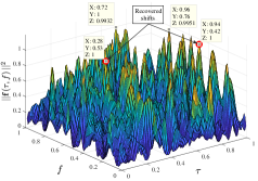
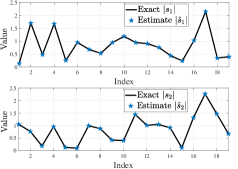
Figure 1: (a) Plot of $||{\bf f}\left({\bf r}\right)||_{2}^{2}$ and the locations of the estimated shifts (denoted by red circles). (b) Comparing the estimated samples of the signals with the true ones.

Once we estimate the shifts, we generate ${\bf a}\left(\hat{{\bf r}}_{j}\right)$ using (7) and then formulate (28). To obtain $\hat{c}_{j}\hat{{\bf h}}_{j}$, we solve (28) using the LS algorithm. Given that we cannot retrieve the phases of $\hat{c}_{j}$, we plot in Fig 1 the magnitudes of the estimated samples $\hat{s}_{j}\left(l\right)$ and we compare them with the true ones. Fig 1 shows that we are able to retrieve the signals samples exactly. Finally, we compute $|{\bf h}_{j}^{H}\hat{{\bf h}}_{j}|$ to find that $|{\bf h}_{1}^{H}\hat{{\bf h}}_{1}|=1-10^{-8}$ and $|{\bf h}_{2}^{H}\hat{{\bf h}}_{2}|=1.0$ which confirms the superiority of the approach.

In the second experiment, we generate the columns of ${\bf D}^{H}$ as [31]

$${\bf d}_{l}=\begin{bmatrix}1,&e^{i2\pi\sigma_{l}},&\ldots,&e^{i2\pi\left(K-1\right)\sigma_{l}}\end{bmatrix}^{T},\ \ \ l=-N,\dots,N,$$

where $\sigma_{l}$ is uniformly distributed in $[0,1]$. We let $L=21$, $K=3$, $R=1$, and we randomly generate the shift pair in $[0,1]^{2}$ which is found to be $\left(0.13,0.67\right)$. Finally, we use the same configurations for ${\bf h}_{j}$ and $c_{j}$ as in the previous scenario.

In Fig 2, we plot $||{\bf f}\left({\bf r}\right)||_{2}^{2}$ in $[0,1]^{2}$. From Fig 2, we can observe that $||{\bf f}\left({\bf r}\right)||_{2}^{2}=1$ at the true shift. Moreover, we plot in Fig 2 the magnitudes of $\hat{s}_{1}\left(l\right)$ and we compare them with the actual ones. Fig 2 shows that the estimated samples coincide with the true ones over all the index range. Finally, we find that $|{\bf h}_{1}^{H}\hat{{\bf h}}_{1}|=1.0$.

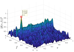
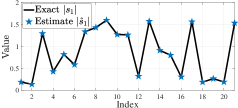
Figure 2: (a) Plot of $||{\bf f}\left({\bf r}\right)||_{2}^{2}$ and the location of the estimated shift. (b) Comparing the estimated samples of the signal with the true ones.

In the third experiment, we consider the case of $K=1$ and we set $L=21$ and $R=3$. The real and the imaginary parts of the entries of ${\bf D}$ are generated from a uniform distribution in $[-1,1]$ while ${\bf h}_{j}$ are set as in the previous scenarios. Moreover, we let the real and the imaginary parts of $c_{j}$ to be fading, i.e., equal to $0.5+w^{2}$ where $w\sim\mathcal{N}\left(0,1\right)$ and we generate their signs uniformly in $[-1,1]$. Finally, the locations of the shifts are set to be $\left(0.8,0.2\right),\left(0.1,0.4\right),$ and $\left(0.7,0.6\right)$. From Fig 3, we can see that our approach recovers the shifts precisely whereas from Fig 3 we can see that the estimated samples coincide with the true ones. Furthermore, we have $|{\bf h}_{1}^{H}\hat{{\bf h}}_{1}|=1+10^{-15}$, $|{\bf h}_{2}^{H}\hat{{\bf h}}_{2}|=1+2\times 10^{-15}$, $|{\bf h}_{3}^{H}\hat{{\bf h}}_{3}|=1-10^{-15}$.

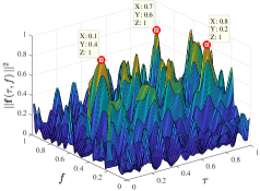
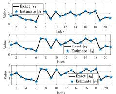
Figure 3: (a) Plot of $||{\bf f}\left({\bf r}\right)||_{2}^{2}$ and the locations of the estimated shifts. (b) Comparing the estimated samples of the signals with the true ones.

Finally, we study the stability of the framework to the noise using simulation with the theoretical analysis being left to future work. Here, we set $L=15,K=3,R=1,$ and we use the same settings in the first scenario for ${\bf D}$ and ${\bf h}_{j}$ and in the previous experiment for $c_{j}$. The shift pair is set at $\left(0.74,0.30\right)$. Then, a Gaussian noise vector $\tilde{{\bf n}}$ is added to ${\bf y}$ at $10$ dB signal-to-noise-ratio (SNR), i.e., SNR (dB) $=10\log_{10}\left(\frac{||{\bf y}||_{2}^{2}}{||\tilde{{\bf n}}||_{2}^{2}}\right)$.

To solve (III-D), we obtain its semidefinite relaxation as

$$\mathcal{P}_{5}:\ \ \ \underset{{\bf q},{\bf Q}}{\text{maximize}}\ \langle{\bf q},{\bf y}\rangle_{\mathbb{R}}-\zeta||{\bf q}||_{2}$$

$$\text{subject to the constraints of (\ref{eq: dual of the dual})}.$$ (29)

In Fig 4, we plot $||{\bf f}\left({\bf r}\right)||_{2}^{2}$ that is obtained by using ${\bf q}$ upon solving (V) with $\zeta=3$. The shift pair at which $||{\bf f}\left({\bf r}\right)||_{2}^{2}=1$ is found to be $\left(0.737,0.298\right)$ which is too close to the original one. Moreover, Fig 4 shows that the magnitudes of the estimated signal samples are close to the original ones with a tenuous error. Finally, we find that $|{\bf h}_{1}^{H}\hat{{\bf h}}_{1}|=0.9674$.

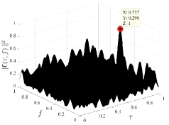
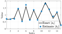
Figure 4: (a) Plot of $||{\bf f}\left({\bf r}\right)||_{2}^{2}$ and the location of the estimated shift. (b) Comparing the estimated samples of the signal with the true ones.

VI Constructing the Dual Vector Polynomial: Proof of Theorem 1

In this section, we prove Theorem 1 by formulating ${\bf f}\left({\bf r}\right)$ that satisfies (22) and (23). Obtaining such polynomial guarantees that the primal optimal solution is equal to ${\bf U}$.

Starting from (21), and based on (22) and (23), our goal is to acquire an expression for ${\bf f}\left({\bf r}\right)$ that satisfies

$${\bf f}\left({\bf r}_{j}\right)=\text{sign}\left(c_{j}\right){\bf h}_{j}\hskip 10.0pt\forall{\bf r}_{j}\in\mathcal{R}$$ (30)

$$- {\bf f}^{\left(1,0\right)}\left({\bf r}_{j}\right)=\bm{0}_{K\times 1}\hskip 17.0pt\forall{\bf r}_{j}\in\mathcal{R}$$ (31)

$$- {\bf f}^{\left(0,1\right)}\left({\bf r}_{j}\right)=\bm{0}_{K\times 1}\hskip 17.0pt\forall{\bf r}_{j}\in\mathcal{R},$$ (32)

where ${\bf f}^{(m^{\prime},n^{\prime})}\left({\bf r}\right):=\frac{\partial^{m^{\prime}}}{\partial\tau^{m^{\prime}}}\frac{\partial^{n^{\prime}}}{\partial f^{n^{\prime}}}{\bf f}\left({\bf r}\right)$. Note that (31) and (32) ensure that ${\bf f}\left({\bf r}\right)$ approaches a local minimum at ${\bf r}_{j}$ which is a necessary condition for (23) to hold. Before formulating ${\bf f}\left({\bf r}\right)$, we recall some related results and definitions in the literature.

In the blind 1D super-resolution (only delay shift), the dual 1D polynomial in [32] guarantees the optimality of the recovery problem. The authors in [32] show that there exists a vector polynomial ${\bf f}_{\text{1D}}\left(\tau\right)$ with: (a) ${\bf f}_{\text{1D}}\left(\tau_{j}\right)=\text{sign}\left(c_{j}\right){\bf h}_{j},\ \forall\tau_{j}\in\mathcal{R}$,  (b) $||{\bf f}_{\text{1D}}\left(\tau_{j}\right)||_{2}<1,\ \forall\tau_{j}\not\in\mathcal{R}$, where $\mathcal{R}$ is the set of the true shifts. This polynomial is formulated by solving a weighted least energy minimization problem and is found to be

$${{\bf f}}_{\text{1D}}\left(\tau\right)=\sum_{j=1}^{R}{\bf M}_{\text{1D}}\left(\tau-\tau_{j}\right)\hbox{\boldmath$\alpha$}_{j}+\sum_{j=1}^{R}{\bf M}_{\text{1D}}^{{}^{\prime}}\left(\tau-\tau_{j}\right)\hbox{\boldmath$\beta$}_{j},$$ (33)

where ${\bf M}_{\text{1D}}\left(\tau\right)\in\mathbb{C}^{K\times K}$ is a random kernel while $\hbox{\boldmath$\alpha$}_{j},\hbox{\boldmath$\beta$}_{j}\in\mathbb{C}^{K\times 1}$ are vector parameters. Finally, ${\bf M}_{\text{1D}}^{{}^{\prime}}\left(\tau\right)$ is the entry-wise derivative of ${\bf M}_{\text{1D}}\left(\tau\right)$ with respect to (w.r.t.) $\tau$.

To show that (33) satisfies (a) and (b) above, the authors first show that under certain assumptions, the expected value of the $m$-th derivative of ${\bf M}_{\text{1D}}\left(\tau\right)$, i.e., $\mathbb{E}\left[{\bf M}_{\text{1D}}^{m}\left(\tau\right)\right]$ is $F^{m}\left(\tau\right){\bf I}_{\text{K}}$ where $F\left(t\right):=\left(\frac{\sin\left(T\pi t\right)}{T\sin\left(\pi t\right)}\right)^{4};T:=\frac{N}{2}+1$ is the squared Fejér kernel. When $N$ is even, the Fejér kernel is a trigonometric polynomial of degree $(T-1)$ and can be written as

$$F\left(t\right)=\frac{1}{T}\sum_{n=-N}^{N}g_{n}e^{i2\pi nt},$$ (34)

where $g_{n}=\frac{1}{T}\sum_{l=\text{max}\{n-T,-T\}}^{\text{min}\{n+T,T\}}\left(1-\frac{|l|}{T}\right)\left(1-\frac{|n-l|}{T}\right).$

Following that, the authors prove that there exist coefficients $\bar{\hbox{\boldmath$\alpha$}}_{j},\bar{\hbox{\boldmath$\beta$}}_{j}\in\mathbb{C}^{K\times 1},j=1,\dots,R$ such that $\bar{{\bf f}}_{\text{1D}}\left(\tau_{j}\right)=\text{sign}\left(c_{j}\right){\bf h}_{j},\forall\tau_{j}\in\mathcal{R}$ and that $||\bar{{\bf f}}_{\text{1D}}\left(\tau_{j}\right)||_{2}<1,\forall\tau_{j}\not\in\mathcal{R},$ where $\bar{{\bf f}}_{\text{1D}}\left(\tau\right):=\mathbb{E}\left[{\bf f}_{\text{1D}}\left(\tau\right)\right]$. Finally, ${\bf f}_{\text{1D}}\left(\tau\right)$ is shown to concentrate around $\bar{{\bf f}}_{\text{1D}}\left(\tau\right)$ anywhere in $[0,1)$ with high probability. The fundamental idea about (33) is that ${\bf M}_{\text{1D}}\left(\tau-\tau_{j}\right)$ interpolates $\text{sign}\left(c_{j}\right){\bf h}_{j}$ while ${\bf M}_{\text{1D}}^{{}^{\prime}}\left(\tau-\tau_{j}\right)$ adapts this interpolation to ensure that local maxima are reached at $\tau_{j}$. This strategy is first developed in [16] and then adapted and applied in different works in the literature, e.g., [17, 31, 18].

Inspired by the previous methodology and other related prior works on super-resolution, e.g., [14, 18, 22, 24], we seek to construct a 2D trigonometric vector polynomial ${\bf f}\left({\bf r}\right)$ that satisfies (22) and (23). However, before going into in-depth technical details, it is essential to first highlight some crucial remarks. First, while (33) is obtained by solving a weighted least energy minimization problem, it is impossible to generalize this problem to the 2D case upon using multiple proper weighting matrices due to nature of the problem formulation. Second, since the 2D dual vector polynomial, the interpolation functions, and the correction functions are all random, we will have to apply probabilist approaches to show that (22) and (23) hold true on our obtained ${\bf f}\left({\bf r}\right)$. Third, given the structure of ${\bf f}\left({\bf r}\right)$ in (24), and unlike (33), we cannot merely use the derivatives of the interpolating matrix as a correction function. This is due to the fact that the derivatives of a polynomial in the form as in (24) do not necessarily have the structure in (24). Finally, we cannot interpolate $\text{sign}\left(c_{j}\right){\bf h}_{j}$ using shifted versions of a single function as shifted versions of a function that represents (24) do not necessarily have the form of (24).

In this paper, we set ${\bf f}\left({\bf r}\right)$ using multiple random kernel matrices ${\bf M}_{\left(m,n\right)}\left({\bf r},{\bf r}_{j}\right)\in\mathbb{C}^{K\times K},m,n=0,1$ in the form

$${\bf f}\left({\bf r}\right)=\sum_{j=1}^{R}{\bf M}_{\left(0,0\right)}\left({\bf r},{\bf r}_{j}\right)\hbox{\boldmath$\alpha$}_{j}+{\bf M}_{\left(1,0\right)}\left({\bf r},{\bf r}_{j}\right)\hbox{\boldmath$\beta$}_{j}$$

$$+{\bf M}_{\left(0,1\right)}\left({\bf r},{\bf r}_{j}\right)\hbox{\boldmath$\gamma$}_{j}.$$ (35)

The key factor of this formulation is to interpolate the vectors $\text{sign}\left(c_{j}\right){\bf h}_{j}$ at ${\bf r}_{j}$ using ${\bf M}_{\left(0,0\right)}\left({\bf r},{\bf r}_{j}\right)$ and then to adjust this interpolation near ${\bf r}_{j}$ by ${\bf M}_{\left(1,0\right)}\left({\bf r},{\bf r}_{j}\right)$ and ${\bf M}_{\left(0,1\right)}\left({\bf r},{\bf r}_{j}\right)$ to ensure that ${\bf f}\left({\bf r}\right)$ approaches local maxima at ${\bf r}_{j}$. The central question here is how to appropriately select the kernel matrices such that ${\bf f}\left({\bf r}\right)$ satisfies (22) and (23). Note that it is clear based on (24) that formulating ${\bf f}\left({\bf r}\right)$ is achieved by finding the proper choice of ${\bf q}$. With all that said, our strategy will be as follows:

• We obtain an initial expression for ${{\bf f}}\left({\bf r}\right)$, i.e., $\hat{{\bf f}}\left({\bf r}\right)$, with

  $$\vspace{-6pt}\hat{{\bf f}}\left({\bf r}\right)=\sum_{p=-N}^{N}[\hat{{\bf q}}]_{p}\widetilde{{\bf D}}_{p}^{H}{\bf a}\left({\bf r}\right),\ \ \hat{{\bf q}}\in\mathbb{C}^{K\times 1};\ \hat{{\bf q}}\neq{\bf q}\vspace{-6pt}$$ (36)

  where $\hat{{\bf q}}$ has unconstrained coefficients which obtained by solving unweighted least energy minimization problem.

• Then, we adapt this formulation by using multiple weighting functions to obtain ${\bf M}_{\left(m,n\right)}\left({\bf r},{\bf r}_{j}\right)$ and ${\bf f}\left({\bf r}\right)$.

• Finally, we dedicate the remaining parts of this section to show that the obtained ${\bf f}\left({\bf r}\right)$ satisfies (22) and (23).

To start with, consider the following linear systems $\forall{\bf r}_{j}\in\mathcal{R}$

$$\hat{{\bf f}}\left({\bf r}_{j}\right)=\text{sign}\left(c_{j}\right){\bf h}_{j},-\hat{{\bf f}}^{\left(1,0\right)}\left({\bf r}_{j}\right)=-\hat{{\bf f}}^{\left(0,1\right)}\left({\bf r}_{j}\right)=\bm{0}_{K\times 1}.$$ (37)

Then, we consider solving the following problem

$$\mathcal{P}_{6}:\ \ \ \underset{\hat{{\bf q}}}{\text{minimize}}\ ||\hat{{\bf q}}||_{2}^{2}\ \ \text{subject to}:(\ref{eq: equations for temp})$$ (38)

By using (36) we can rewrite (38) as

$$\mathcal{P}_{7}:\ \ \ \underset{\hat{{\bf q}}}{\text{minimize}}||\hat{{\bf q}}||_{2}^{2}\ \ \ \text{subject to}:\ \ {\bf F}\hat{{\bf q}}={\bf g},$$ (39)

where ${\bf F}\in\mathbb{C}^{3RK\times L}$ is given by

$${\bf F}={\begin{bmatrix}\widetilde{{\bf D}}_{-N}^{H}{\bf a}\left({\bf r}_{1}\right)&\ldots&\widetilde{{\bf D}}_{N}^{H}{\bf a}\left({\bf r}_{1}\right)\\ \vdots&\vdots\\ \widetilde{{\bf D}}_{-N}^{H}{\bf a}\left({\bf r}_{R}\right)&\ldots&\widetilde{{\bf D}}_{N}^{H}{\bf a}\left({\bf r}_{R}\right)\\ -\widetilde{{\bf D}}_{-N}^{H}{\bf a}^{\left(1,0\right)}\left({\bf r}\right)|_{{\bf r}={\bf r}_{1}}&\ldots&-\widetilde{{\bf D}}_{N}^{H}{\bf a}^{\left(1,0\right)}\left({\bf r}\right)|_{{\bf r}={\bf r}_{1}}\\ \vdots&\vdots\\ -\widetilde{{\bf D}}_{-N}^{H}{\bf a}^{\left(1,0\right)}\left({\bf r}\right)|_{{\bf r}={\bf r}_{R}}&\ldots&-\widetilde{{\bf D}}_{N}^{H}{\bf a}^{\left(1,0\right)}\left({\bf r}\right)|_{{\bf r}={\bf r}_{R}}\\ -\widetilde{{\bf D}}_{-N}^{H}{\bf a}^{\left(0,1\right)}\left({\bf r}\right)|_{{\bf r}={\bf r}_{1}}&\ldots&-\widetilde{{\bf D}}_{N}^{H}{\bf a}^{\left(0,1\right)}\left({\bf r}\right)|_{{\bf r}={\bf r}_{1}}\\ \vdots&\vdots\\ -\widetilde{{\bf D}}_{-N}^{H}{\bf a}^{\left(0,1\right)}\left({\bf r}\right)|_{{\bf r}={\bf r}_{R}}&\ldots&-\widetilde{{\bf D}}_{N}^{H}{\bf a}^{\left(0,1\right)}\left({\bf r}\right)|_{{\bf r}={\bf r}_{R}}\end{bmatrix}}$$

while ${\bf g}=\begin{bmatrix}\text{sign}\left(c_{1}\right){\bf h}_{1}^{T},\ldots,\text{sign}\left(c_{R}\right){\bf h}_{R}^{T},\bm{0}_{K\times 1}^{T},\ldots,\bm{0}_{K\times 1}^{T}\end{bmatrix}^{T}$ $\in\mathbb{C}^{3RK\times 1}$. Using the KKT optimality conditions [40, Section 5.5.3], we can show that the solution of (39) is

$$\hat{{\bf q}}={\bf F}^{H}{\bf v},$$ (40)

where ${\bf v}=\begin{bmatrix}\hbox{\boldmath$\alpha$}^{T},\hbox{\boldmath$\beta$}^{T},\hbox{\boldmath$\gamma$}^{T}\end{bmatrix}^{T}$ with $\hbox{\boldmath$\alpha$}=\begin{bmatrix}\hbox{\boldmath$\alpha$}_{1}^{T},\dots,\hbox{\boldmath$\alpha$}_{R}^{T}\end{bmatrix}^{T}$, $\hbox{\boldmath$\beta$}=\begin{bmatrix}\hbox{\boldmath$\beta$}_{1}^{T},\dots,\hbox{\boldmath$\beta$}_{R}^{T}\end{bmatrix}^{T}$, $\hbox{\boldmath$\gamma$}=\begin{bmatrix}\hbox{\boldmath$\gamma$}_{1}^{T},\dots,\hbox{\boldmath$\gamma$}_{R}^{T}\end{bmatrix}^{T}$ such that $\hbox{\boldmath$\alpha$}_{j},\hbox{\boldmath$\beta$}_{j},\hbox{\boldmath$\gamma$}_{j}\in\mathbb{C}^{K\times 1}$. By substituting for ${\bf F}$ and ${\bf v}$ in (40) we obtain

$$\hat{{\bf q}} =\sum_{j=1}^{R}\left(\begin{bmatrix}{\bf a}\left({\bf r}_{j}\right)^{H}\widetilde{{\bf D}}_{-N}\\ \vdots\\ {\bf a}\left({\bf r}_{j}\right)^{H}\widetilde{{\bf D}}_{N}\end{bmatrix}\hbox{\boldmath$\alpha$}_{j}-\begin{bmatrix}{\bf a}^{\left(1,0\right)}\left({\bf r}\right)^{H}|_{{\bf r}={\bf r}_{j}}\widetilde{{\bf D}}_{-N}\\ \vdots\\ {\bf a}^{\left(1,0\right)}\left({\bf r}\right)^{H}|_{{\bf r}={\bf r}_{j}}\widetilde{{\bf D}}_{N}\end{bmatrix}\hbox{\boldmath$\beta$}_{j}\right.$$

$$\left.-\begin{bmatrix}{\bf a}^{\left(0,1\right)}\left({\bf r}\right)^{H}|_{{\bf r}={\bf r}_{j}}\widetilde{{\bf D}}_{-N}\\ \vdots\\ {\bf a}^{\left(0,1\right)}\left({\bf r}\right)^{H}|_{{\bf r}={\bf r}_{j}}\widetilde{{\bf D}}_{N}\end{bmatrix}\hbox{\boldmath$\gamma$}_{j}\right).$$ (41)

Now we substitute (VI) in (36) and manipulate to obtain

$$\hat{{\bf f}}\left({\bf r}\right) =\sum_{j=1}^{R}\left[\left(\sum_{p=-N}^{N}\widetilde{{\bf D}}_{p}^{H}{\bf a}\left({\bf r}\right){\bf a}^{(0,0)}\left({\bf r}\right)^{H}|_{{\bf r}={\bf r}_{j}}\widetilde{{\bf D}}_{p}\right)\hbox{\boldmath$\alpha$}_{j}\right.$$

$$+\left.\left(-\sum_{p=-N}^{N}\widetilde{{\bf D}}_{p}^{H}{\bf a}\left({\bf r}\right){\bf a}^{\left(1,0\right)}\left({\bf r}\right)^{H}|_{{\bf r}={\bf r}_{j}}\widetilde{{\bf D}}_{p}\right)\hbox{\boldmath$\beta$}_{j}\right.$$

$$\left.+\left(-\sum_{p=-N}^{N}\widetilde{{\bf D}}_{p}^{H}{\bf a}\left({\bf r}\right){\bf a}^{\left(0,1\right)}\left({\bf r}\right)^{H}|_{{\bf r}={\bf r}_{j}}\widetilde{{\bf D}}_{p}\right)\hbox{\boldmath$\gamma$}_{j}\right].$$ (42)

Upon defining the matrix $\widehat{{\bf M}}^{(m^{\prime},n^{\prime})}\left({\bf r},{\bf r}_{j}\right)\in\mathbb{C}^{K\times K}$ such that

$$\widehat{{\bf M}}^{(m^{\prime},n^{\prime})}\left({\bf r},{\bf r}_{j}\right)=-1^{m^{\prime}+n^{\prime}}\sum_{p=-N}^{N}\widetilde{{\bf D}}_{p}^{H}{\bf a}\left({\bf r}\right){\bf a}^{(m^{\prime},n^{\prime})}\left({\bf r}_{j}\right)^{H}\widetilde{{\bf D}}_{p}$$ (43)

we can rewrite (VI) as

$$\hat{{\bf f}}\left({\bf r}\right)=\sum_{j=1}^{R} \widehat{{\bf M}}^{(0,0)}\left({\bf r},{\bf r}_{j}\right)\hbox{\boldmath$\alpha$}_{j}+\widehat{{\bf M}}^{(1,0)}\left({\bf r},{\bf r}_{j}\right)\hbox{\boldmath$\beta$}_{j}$$ (44)

$$+\widehat{{\bf M}}^{(0,1)}\left({\bf r},{\bf r}_{j}\right)\hbox{\boldmath$\gamma$}_{j}.\vspace{-8pt}$$

which provides the initial formulation for ${\bf f}\left({\bf r}\right)$ as in (36). Now, we can turn our attention into obtaining ${\bf M}_{\left(m,n\right)}\left({\bf r},{\bf r}_{j}\right)$ and as a result ${\bf f}\left({\bf r}\right)$ by adapting (43). Following that, we will provide our justifications for this proposed adaptation.

To start with, consider ${\bf z}_{p}\left({\bf r}\right)_{\left(m,n\right)}\in\mathbb{C}^{L^{2}\times 1}$ such that

$$[{\bf z}_{p}\left({\bf r}_{j}\right)_{\left(m,n\right)}]_{(\left(k,l\right),1)}:=g_{k}\left(i2\pi k\right)^{m}g_{p}\left(i2\pi p\right)^{n}e^{\frac{i2\pi k\left(p+l\right)}{L}}\times$$

$$e^{-i2\pi\left(k\tau_{j}+pf_{j}\right)};\ \ \ p,k,l=-N,\dots,N;\ \ m,n=0,1.$$ (45)

Based on (VI), we propose formulating our kernel matrix as

$${\bf M}_{\left(m,n\right)}\left({\bf r},{\bf r}_{j}\right):=\frac{1}{T^{2}}\sum_{p=-N}^{N}\widetilde{{\bf D}}_{p}^{H}{\bf a}\left({\bf r}\right){\bf z}_{p}\left({\bf r}_{j}\right)_{\left(m,n\right)}^{H}\widetilde{{\bf D}}_{p}.$$ (46)

By using (VI) and (8) we can show that

$${\bf z}_{p}\left({\bf r}_{j}\right)_{\left(m,n\right)}^{H}\widetilde{{\bf D}}_{p}=\sum_{l,k=-N}^{N} g_{k}\left(-i2\pi k\right)^{m}g_{p}\left(-i2\pi p\right)^{n}e^{\frac{-i2\pi kl}{L}}\times$$

$$e^{i2\pi\left(k\tau_{j}+pf_{j}\right)}{\bf d}_{\left(p-l\right)}^{H}.$$ (47)

Moreover, we can also deduce that

$${\bf a}\left({\bf r}\right)^{H}\widetilde{{\bf D}}_{p}=\frac{1}{L}\sum_{l,k=-N}^{N}e^{\frac{-i2\pi kl}{L}}e^{i2\pi\left(k\tau+pf\right)}{\bf d}^{H}_{\left(p-l\right)}.$$ (48)

Now from (VI) and (48) we can write

$${\bf M}_{\left(m,n\right)}\left({\bf r},{\bf r}_{j}\right)=$$

$$\frac{1}{L}\sum_{p=-N}^{N}\frac{1}{T^{2}}\sum_{l,l^{\prime},k,k^{\prime}=-N}^{N}g_{k^{\prime}}\left(-i2\pi k^{\prime}\right)^{m}g_{p}\left(-i2\pi p\right)^{n}\times$$

$$e^{i2\pi\frac{\left(kl-k^{\prime}l^{\prime}\right)}{L}}e^{-i2\pi\left(k\tau-k^{\prime}\tau_{j}\right)}e^{-i2\pi p\left(f-f_{j}\right)}{\bf d}_{\left(p-l\right)}{\bf d}_{\left(p-l^{\prime}\right)}^{H}.$$ (49)

On the other hand, we can also show that

$$\widehat{{\bf M}}^{(0,0)}\left({\bf r},{\bf r}_{j}\right) =\sum_{p=-N}^{N}\frac{1}{L^{2}}\sum_{l,l^{\prime},k,k^{\prime}=-N}^{N}e^{i2\pi\frac{\left(kl-k^{\prime}l^{\prime}\right)}{L}}\times$$

$$e^{-i2\pi\left(k\tau-k^{\prime}\tau_{j}\right)}e^{-i2\pi p\left(f-f_{j}\right)}{\bf d}_{\left(p-l\right)}{\bf d}^{H}_{\left(p-l^{\prime}\right)}.$$ (50)

Since ${\bf f}\left({\bf r}\right)$ is a linear combinations of ${\bf M}_{\left(m,n\right)}\left({\bf r},{\bf r}_{j}\right)$, it is easy to show that it has the form in (24) as required. Comparing ${\bf M}_{\left(m,n\right)}\left({\bf r},{\bf r}_{j}\right)$ with $\widehat{{\bf M}}^{(0,0)}\left({\bf r},{\bf r}_{j}\right)$, we can see that ${\bf M}_{\left(m,n\right)}\left({\bf r},{\bf r}_{j}\right)$ is a scaled version of $\widehat{{\bf M}}^{(0,0)}\left({\bf r},{\bf r}_{j}\right)$. The appointed choice of ${\bf M}_{\left(m,n\right)}\left({\bf r},{\bf r}_{j}\right)$, as we will show in Section VI-A, is motivated by the fact that it concentrates around its average deterministic version $\mathbb{E}[{{\bf M}}_{\left(m,n\right)}\left({\bf r},{\bf r}_{j}\right)]$ in Euclidean norm measure with high probability. This fact is crucial in showing that (22) is satisfied (as will be shown in Section VI-B) and is also found to facilitate the proofs and to yield nicely constants. More importantly, the expression of ${\bf M}_{\left(m,n\right)}\left({\bf r},{\bf r}_{j}\right)$, as we will show in the remaining parts of this section, provides ${\bf f}\left({\bf r}\right)$ that satisfies (22) and (23), which then guarantees the existence of the dual optimal solution and thus our required primal optimal solution ${\bf U}$. We point out that anyone might suggest and use different formulation for the kernel matrices as long as they provide ${\bf f}\left({\bf r}\right)$ that satisfies (22) and (23) and follow the same proof techniques that will be provided in this paper. Finally, by substituting (46) in (VI) we can formulate our dual trigonometric vector polynomial ${\bf f}\left({\bf r}\right)$.

Before closing this part, we will express the derivatives of ${\bf M}_{\left(m,n\right)}\left({\bf r},{\bf r}_{j}\right)$, i.e., ${\bf M}^{(m^{\prime},n^{\prime})}_{\left(m,n\right)}\left({\bf r},{\bf r}_{j}\right)$, in a matrix-vector form that involves ${\bf D}$ to facilitate our proofs later. For that, let us first define a modified version of (7) as

$$\left[{\bf a}_{p}\left({\bf r}\right)\right]_{(\left(k,l\right),1)}= D_{N}\left(\frac{k}{L}-f\right)D_{N}\left(\frac{p-l}{L}-\tau\right),$$ (51)

with $p=-N,\dots,N$. From the periodicity property we write

$$\widetilde{{\bf D}}_{p}^{H}{\bf a}\left({\bf r}\right)=\widehat{{\bf D}}_{p}^{H}{\bf a}_{p}\left({\bf r}\right),$$ (52)

where $[\widehat{{\bf D}}_{p}]_{(\left(k,l\right),1\to K)}={\bf d}_{l}^{H}e^{\frac{i2\pi pk}{L}}$. Moreover, define the block diagonal matrix ${\bf J}_{p}\in\mathbb{C}^{L^{2}\times L^{2}}$ as

$${\bf J}_{p}=\text{diag}\left(\left({\bf J}_{p}^{-N},\dots,{\bf J}_{p}^{N}\right)\right),$$ (53)

where ${\bf J}_{p}^{k}:=e^{\frac{-i2\pi pk}{L}}{\bf I}_{\text{L}},\ \ k=-N,\dots,N.$ Finally, let

$${\bf O}:=\left[{\bf I}_{\text{L}}^{-N},\dots,{\bf I}_{\text{L}}^{N}\right]\in\mathbb{R}^{L\times L^{2}}.$$ (54)

Based on (3), (52), (53), and (54), we can write

$$\widetilde{{\bf D}}_{p}^{H}{\bf a}\left({\bf r}\right)=\widehat{{\bf D}}_{p}^{H}{\bf a}_{p}\left({\bf r}\right)={\bf D}^{H}{\bf O}{\bf J}_{p}{\bf a}_{p}\left({\bf r}\right).$$ (55)

Now, we can rewrite the derivatives of (46) using (55) as

$${\bf M}^{(m^{\prime},n^{\prime})}_{\left(m,n\right)}\left({\bf r},{\bf r}_{j}\right)=$$

$${\bf D}^{H}\left[\frac{1}{T^{2}}\sum_{p=-N}^{N}{\bf O}{\bf J}_{p}{\bf a}_{p}^{(m^{\prime},n^{\prime})}\left({\bf r}\right)\tilde{{\bf z}}_{p}\left({\bf r}_{j}\right)_{\left(m,n\right)}^{H}{\bf J}_{p}^{H}{\bf O}^{H}\right]{\bf D}$$ (56)

$$=:{\bf D}^{H}{\bf R}_{(m,n)}^{(m^{\prime},n^{\prime})}\left({\bf r},{\bf r}_{j}\right){\bf D},$$ (57)

where $\tilde{{\bf z}}_{p}\left({\bf r}_{j}\right)_{\left(m,n\right)}$ is obtained by replacing $l$ with $p-l$ in (VI) while the matrix ${\bf R}_{(m,n)}^{(m^{\prime},n^{\prime})}\left({\bf r},{\bf r}_{j}\right)\in\mathbb{C}^{L\times L}$ refers to the terms between the square brackets in (VI) with $m^{\prime},n^{\prime}=0,1$.

VI-A Showing that $\Big{|}\Big{|}{\bf M}^{(m^{\prime},n^{\prime})}_{\left(m,n\right)}\left({\bf r},{\bf r}_{j}\right)-\mathbb{E}\left[{\bf M}^{(m^{\prime},n^{\prime})}_{\left(m,n\right)}\left({\bf r},{\bf r}_{j}\right)\right]\Big{|}\Big{|}_{2}$ is small

In this section, we show that the our kernel matrix concentrates around its mean with high probability under certain conditions. For that, we show in Appendix D that

$$\mathbb{E}\left[{\bf M}_{\left(m,n\right)}^{(m^{\prime},n^{\prime})}\left({\bf r},{\bf r}_{j}\right)\right] =F^{(m+m^{\prime})}\left(\tau-\tau_{j}\right)F^{(n+n^{\prime})}\left(f-f_{j}\right){\bf I}_{\text{K}}$$

$$=:\macc@depth\char 1\relax\frozen@everymath{\macc@group}\macc@set@skewchar\macc@nested@a 111{M}^{\left(m+m^{\prime},n+n^{\prime}\right)}\left({\bf r}-{\bf r}_{j}\right){\bf I}_{\text{K}}$$

where $F\left(t\right)$ is given by (34). Now, if we recall that the $i$-th column of ${\bf D}$ is denoted by $\hat{{\bf d}}_{i}\in\mathbb{C}^{L\times 1}$, we can express the element at $(i^{\prime},j^{\prime})$ location in ${\bf M}^{(m^{\prime},n^{\prime})}_{\left(m,n\right)}\left({\bf r},{\bf r}_{j}\right)$ using (57) by

$$\left[{\bf M}^{(m^{\prime},n^{\prime})}_{\left(m,n\right)}\left({\bf r},{\bf r}_{j}\right)\right]_{(i^{\prime},j^{\prime})}=\hat{{\bf d}}_{i^{\prime}}^{H}{\bf R}_{(m,n)}^{(m^{\prime},n^{\prime})}\left({\bf r},{\bf r}_{j}\right)\hat{{\bf d}}_{j^{\prime}}.$$ (58)

Moreover, we can conclude based on (VI-A) and (58) that

$$\mathbb{E}\left[\hat{{\bf d}}_{i^{\prime}}^{H}{\bf R}_{(m,n)}^{(m^{\prime},n^{\prime})}\left({\bf r},{\bf r}_{j}\right)\hat{{\bf d}}_{i^{\prime}}\right]=F^{(m+m^{\prime})}\left(\tau-\tau_{j}\right)F^{(n+n^{\prime})}\left(f-f_{j}\right)$$

and

$$\mathbb{E}\left[\hat{{\bf d}}_{i^{\prime}}^{H}{\bf R}_{(m,n)}^{(m^{\prime},n^{\prime})}\left({\bf r},{\bf r}_{j}\right)\hat{{\bf d}}_{j^{\prime}}\right]=0,\forall i^{\prime},j^{\prime}=1,\dots,K:i^{\prime}\neq j^{\prime}.$$

Lemma 1.

Let ${\bf r},{\bf r}_{j}\in[0,1]^{2},j=1,\dots,R$ and recall ${\bf M}_{(m,n)}^{(m^{\prime},n^{\prime})}\left({\bf r},{\bf r}_{j}\right)$ in (57) with $m,m^{\prime},n,n^{\prime}=0,1$ and $m+m^{\prime}+n+n^{\prime}\leq 2$. Then, for every real $\epsilon_{1}>0,\delta>0$ the event $\mathcal{E}_{1}=\left\{\frac{1}{\mu^{m+m^{\prime}+n+n^{\prime}}}\bigg{|}\bigg{|}{\bf M}_{(m,n)}^{(m^{\prime},n^{\prime})}\left({\bf r},{\bf r}_{j}\right)\mathbb{E}\left[{\bf M}_{(m,n)}^{(m^{\prime},n^{\prime})}\left({\bf r},{\bf r}_{j}\right)\right]\bigg{|}\bigg{|}_{2}\leq\epsilon_{1}\right\}$ occurs with probability $\text{Pr}\left[\mathcal{E}_{1}\right]\geq 1-\delta/2R^{2}$ provided that

$$L\geq\frac{C_{1}^{2}}{\epsilon_{1}^{2}}RK\widetilde{K}^{4}\log^{2}\left(\frac{4R^{2}K^{2}}{\delta}\right),$$ (59)

where $\mu:=\sqrt{|F^{\prime\prime}\left(0\right)|}$ and $C_{1}$ is a numerical constant.

The proof of Lemma 1 relies on Lemma 4 which is built on top of Lemmas 2 and 3 below.

Lemma 2.

[44, Theorem 1.1], [45, Theorem 2.3] Let ${\bf u}\in\mathbb{C}^{N_{1}\times 1}$ be a random vector satisfying (13), (14) with ${\bf I}_{\text{N}_{1}}$, and (15). Then, for any $N_{1}\times N_{1}$ matrix ${\bf A}$ and $t>0$ we have

$$\text{Pr}\left[\left|{\bf u}^{H}{\bf A}{\bf u}-\mathbb{E}\left[{\bf u}^{H}{\bf A}{\bf u}\right]\right|\geq t\right]\leq$$

$$2\exp\left(-\frac{1}{C}\min\left(\frac{t^{2}}{2\widetilde{K}^{4}||{\bf A}||_{F}^{2}},\frac{t}{\widetilde{K}^{2}||{\bf A}||_{2}}\right)\right),$$ (60)

where $C$ is a constant. Furthermore, let ${\bf v}\in\mathbb{C}^{N_{1}\times 1}$ be another random vector that is independent of ${\bf u}$ and satisfies (13), (14) with ${\bf I}_{\text{N}_{1}}$, and (15). Then, the following inequality holds true (adapted from [44, Theorem 1.1] and [46, Theorem 2.1])

$$\text{Pr}\left[\left|{\bf u}^{H}{\bf A}{\bf v}-\mathbb{E}\left[{\bf u}^{H}{\bf A}{\bf v}\right]\right|\geq t\right]\leq$$

$$2\exp\left(-\frac{1}{C}\min\left(\frac{t^{2}}{2||{\bf A}||_{F}^{2}},\frac{t}{||{\bf A}||_{2}}\right)\right).$$ (61)

Note that the results in [44, 45, 46] are originally obtained for real random vectors. However, using standard complexification tricks, we can easily obtain their complex versions as in (2) and (2) (see the proof of [44, Theorem 1.1] for more details).

Lemma 3.

Recall (57) with $j=1,\dots,R$, then

$$\big{|}\big{|}{\bf R}_{(m,n)}^{(m^{\prime},n^{\prime})}\left({\bf r},{\bf r}_{j}\right)\big{|}\big{|}_{F}\leq\frac{C_{2}}{\sqrt{L}}\left(2\pi N\right)^{(m+m^{\prime}+n+n^{\prime})},$$ (62)

where $m,m^{\prime},n,n^{\prime}=0,1$ and $C_{2}$ is a numerical constant.

The proof of Lemma 3 follows that in [18, Lemma 3] and is provided in Appendix E.

In Lemma 4 below, we apply Lemmas 2 and 3 to show that each element in ${\bf M}^{(m^{\prime},n^{\prime})}_{\left(m,n\right)}\left({\bf r},{\bf r}_{j}\right)$ is close to its corresponding one in $\mathbb{E}[{\bf M}_{\left(m,n\right)}^{(m^{\prime},n^{\prime})}\left({\bf r},{\bf r}_{j}\right)]$ with very probability. Then, we use matrix inequalities and the union-bound along with Lemma 4 to prove Lemma 1. Here, we point out that based on Assumption 1, $\hat{{\bf d}}_{i}$ also satisfies (13) and (14) with ${\bf I}_{\text{L}}$.

Lemma 4.

Let ${\bf r},{\bf r}_{j}\in[0,1]^{2}$ and recall (58) with $m$, $m^{\prime}$, $n$, $n^{\prime}$= 0, 1 and $m+m^{\prime}+n+n^{\prime}\leq 2$. Then, for any real $\alpha>0$, the following two probability measures hold true

$$\text{Pr}\left[\frac{1}{\mu^{m+m^{\prime}+n+n^{\prime}}}\Big{|}\hat{{\bf d}}_{i^{\prime}}^{H}{\bf R}_{(m,n)}^{(m^{\prime},n^{\prime})}\left({\bf r},{\bf r}_{j}\right)\hat{{\bf d}}_{i^{\prime}}-\right.$$

$$\left.\mathbb{E}\left[\hat{{\bf d}}_{i^{\prime}}^{H}{\bf R}_{(m,n)}^{(m^{\prime},n^{\prime})}\left({\bf r},{\bf r}_{j}\right)\hat{{\bf d}}_{i^{\prime}}\right]\Big{|}\geq C_{2}12^{\frac{m+m^{\prime}+n+n^{\prime}}{2}}\frac{\alpha}{\sqrt{L}}\right]$$

$$\leq 2\exp\left(-\frac{1}{C}\min\left(\frac{\alpha^{2}}{2\widetilde{K}^{4}},\frac{\alpha}{\widetilde{K}^{2}}\right)\right),\forall i^{\prime}=1,\dots,K$$ (63)

$$\text{Pr}\left[\frac{1}{\mu^{m+m^{\prime}+n+n^{\prime}}}\Big{|}\hat{{\bf d}}_{i^{\prime}}^{H}{\bf R}_{(m,n)}^{(m^{\prime},n^{\prime})}\left({\bf r},{\bf r}_{j}\right)\hat{{\bf d}}_{j^{\prime}}-\right.$$

$$\left.\mathbb{E}\left[\hat{{\bf d}}_{i^{\prime}}^{H}{\bf R}_{(m,n)}^{(m^{\prime},n^{\prime})}\left({\bf r},{\bf r}_{j}\right)\hat{{\bf d}}_{j^{\prime}}\right]\Big{|}\geq C_{2}12^{\frac{m+m^{\prime}+n+n^{\prime}}{2}}\frac{\alpha}{\sqrt{L}}\right]\leq$$

$$2\exp{\left(-\frac{1}{C}\min\left(\frac{\alpha^{2}}{2},\alpha\right)\right)},\forall i^{\prime},j^{\prime}=1,\dots,K:i^{\prime}\neq j^{\prime}.$$ (64)

The proof of Lemma 4 is given in Appendix F.

Now we can prove Lemma 1 as in Appendix G.

VI-B Showing that ${\bf f}\left({\bf r}\right)$ satisfies (22): Obtaining $\hbox{\boldmath$\alpha$}_{j},\hbox{\boldmath$\beta$}_{j}$, and $\hbox{\boldmath$\gamma$}_{j}$

To prove that (22) holds, it is enough to show that there exists $\hbox{\boldmath$\alpha$}_{j},\hbox{\boldmath$\beta$}_{j}$, $\hbox{\boldmath$\gamma$}_{j}$ such that ${\bf f}\left({\bf r}\right)$ in (VI) satisfies (22) with high probability. For that, we first write

$${\bf f}^{(m^{\prime},n^{\prime})}\left({\bf r}\right)=\sum_{j=1}^{R} {\bf M}^{(m^{\prime},n^{\prime})}_{\left(0,0\right)}\left({\bf r},{\bf r}_{j}\right)\hbox{\boldmath$\alpha$}_{j}+{\bf M}^{(m^{\prime},n^{\prime})}_{\left(1,0\right)}\left({\bf r},{\bf r}_{j}\right)\hbox{\boldmath$\beta$}_{j}$$

$$+{\bf M}^{(m^{\prime},n^{\prime})}_{\left(0,1\right)}\left({\bf r},{\bf r}_{j}\right)\hbox{\boldmath$\gamma$}_{j},$$ (65)

where $m^{\prime},n^{\prime}=0,1$. Moreover, we can write based on (VI-A)

$$\bar{{\bf f}}^{(m^{\prime},n^{\prime})}\left({\bf r}\right):=\mathbb{E}\left[{\bf f}^{(m^{\prime},n^{\prime})}\left({\bf r}\right)\right]=\sum_{j=1}^{R}\macc@depth\char 1\relax\frozen@everymath{\macc@group}\macc@set@skewchar\macc@nested@a 111{M}^{(m^{\prime},n^{\prime})}\left({\bf r}-{\bf r}_{j}\right)\bar{\hbox{\boldmath$\alpha$}}_{j}$$

$$+\macc@depth\char 1\relax\frozen@everymath{\macc@group}\macc@set@skewchar\macc@nested@a 111{M}^{(m^{\prime}+1,n^{\prime})}\left({\bf r}-{\bf r}_{j}\right)\bar{\hbox{\boldmath$\beta$}}_{j}+\macc@depth\char 1\relax\frozen@everymath{\macc@group}\macc@set@skewchar\macc@nested@a 111{M}^{(m^{\prime},n^{\prime}+1)}\left({\bf r}-{\bf r}_{j}\right)\bar{\hbox{\boldmath$\gamma$}}_{j},$$ (66)

where $\bar{\hbox{\boldmath$\alpha$}}_{j},\bar{\hbox{\boldmath$\beta$}}_{j},\bar{\hbox{\boldmath$\gamma$}}_{j}\in\mathbb{C}^{K\times 1}$ are the solutions of the equations

$$\bar{{\bf f}}\left({\bf r}_{j}\right)=\text{sign}\left(c_{j}\right){\bf h}_{j},-\bar{{\bf f}}^{\left(1,0\right)}\left({\bf r}_{j}\right)=-\bar{{\bf f}}^{\left(0,1\right)}\left({\bf r}_{j}\right)=\bm{0}_{K\times 1},$$ (67)

$\forall{\bf r}_{j}\in\mathcal{R}$. Starting from (VI-B), we write (30), (31), and (32) as

$$\underbrace{{\begin{bmatrix}{\bf E}^{(0,0)}_{(0,0)}&\frac{1}{\mu}{\bf E}^{(0,0)}_{(1,0)}&\frac{1}{\mu}{\bf E}^{(0,0)}_{(0,1)}\\ -\frac{1}{\mu}{\bf E}^{(1,0)}_{(0,0)}&-\frac{1}{\mu^{2}}{\bf E}^{(1,0)}_{(1,0)}&-\frac{1}{\mu^{2}}{\bf E}^{(1,0)}_{(0,1)}\\ -\frac{1}{\mu}{\bf E}^{(0,1)}_{(0,0)}&-\frac{1}{\mu^{2}}{\bf E}^{(0,1)}_{(1,0)}&-\frac{1}{\mu^{2}}{\bf E}^{(0,1)}_{(0,1)}\end{bmatrix}}}_{{\bf E}}\begin{bmatrix}{\hbox{\boldmath$\alpha$}}\\ \mu{\hbox{\boldmath$\beta$}}\\ \mu{\hbox{\boldmath$\gamma$}}\end{bmatrix}=\begin{bmatrix}{\bf h}\\ \bm{0}_{RK\times 1}\\ \bm{0}_{RK\times 1}\end{bmatrix}$$ (68)

where ${\bf E}^{(m^{\prime},n^{\prime})}_{(m,n)}\in\mathbb{C}^{RK\times RK}$ consists of $R\times R$ block matrices of size $K\times K$ with the one at the $\left(l,k\right)$ location being given by $[{\bf E}^{(m^{\prime},n^{\prime})}_{(m,n)}]_{(l,k)}:={\bf M}^{(m^{\prime},n^{\prime})}_{(m,n)}\left({\bf r}_{l},{\bf r}_{k}\right)$ (see (I.1) in Appendix I) while ${\bf h}:=\left[\text{sign}\left(c_{1}\right){\bf h}_{1}^{T},\ldots,\text{sign}\left(c_{R}\right){\bf h}_{R}^{T}\right]^{T}\in\mathbb{C}^{RK\times 1}$.

Moreover, we can express (67) using (VI-B) as

$$\left(\macc@depth\char 1\relax\frozen@everymath{\macc@group}\macc@set@skewchar\macc@nested@a 111{{\bf E}}\otimes{\bf I}_{\text{K}}\right)\begin{bmatrix}\bar{\hbox{\boldmath$\alpha$}}\\ \mu\bar{\hbox{\boldmath$\beta$}}\\ \mu\bar{\hbox{\boldmath$\gamma$}}\end{bmatrix}=\begin{bmatrix}{\bf h}\\ \bm{0}_{RK\times 1}\\ \bm{0}_{RK\times 1}\end{bmatrix},$$ (69)

where $\macc@depth\char 1\relax\frozen@everymath{\macc@group}\macc@set@skewchar\macc@nested@a 111{{\bf E}}\in\mathbb{C}^{3R\times 3R}$ is given by

$$\macc@depth\char 1\relax\frozen@everymath{\macc@group}\macc@set@skewchar\macc@nested@a 111{{\bf E}}={\begin{bmatrix}\macc@depth\char 1\relax\frozen@everymath{\macc@group}\macc@set@skewchar\macc@nested@a 111{{\bf E}}^{(0,0)}&\frac{1}{\mu}\macc@depth\char 1\relax\frozen@everymath{\macc@group}\macc@set@skewchar\macc@nested@a 111{{\bf E}}^{(1,0)}&\frac{1}{\mu}\macc@depth\char 1\relax\frozen@everymath{\macc@group}\macc@set@skewchar\macc@nested@a 111{{\bf E}}^{(0,1)}\\ -\frac{1}{\mu}\macc@depth\char 1\relax\frozen@everymath{\macc@group}\macc@set@skewchar\macc@nested@a 111{{\bf E}}^{(1,0)}&-\frac{1}{\mu^{2}}\macc@depth\char 1\relax\frozen@everymath{\macc@group}\macc@set@skewchar\macc@nested@a 111{{\bf E}}^{(2,0)}&-\frac{1}{\mu^{2}}\macc@depth\char 1\relax\frozen@everymath{\macc@group}\macc@set@skewchar\macc@nested@a 111{{\bf E}}^{(1,1)}\\ -\frac{1}{\mu}\macc@depth\char 1\relax\frozen@everymath{\macc@group}\macc@set@skewchar\macc@nested@a 111{{\bf E}}^{(0,1)}&-\frac{1}{\mu^{2}}\macc@depth\char 1\relax\frozen@everymath{\macc@group}\macc@set@skewchar\macc@nested@a 111{{\bf E}}^{(1,1)}&-\frac{1}{\mu^{2}}\macc@depth\char 1\relax\frozen@everymath{\macc@group}\macc@set@skewchar\macc@nested@a 111{{\bf E}}^{(0,2)}\end{bmatrix}}$$ (70)

with $[\macc@depth\char 1\relax\frozen@everymath{\macc@group}\macc@set@skewchar\macc@nested@a 111{{\bf E}}^{(m^{\prime},n^{\prime})}]_{(l,k)}:=\macc@depth\char 1\relax\frozen@everymath{\macc@group}\macc@set@skewchar\macc@nested@a 111{M}^{(m^{\prime},n^{\prime})}\left({\bf r}_{l}-{\bf r}_{k}\right)$ while $\bar{\hbox{\boldmath$\alpha$}}:=[\bar{\hbox{\boldmath$\alpha$}}_{1}^{T},\dots,\bar{\hbox{\boldmath$\alpha$}}_{R}^{T}]^{T},\bar{\hbox{\boldmath$\beta$}}:=[\bar{\hbox{\boldmath$\beta$}}_{1}^{T},\dots,\bar{\hbox{\boldmath$\beta$}}_{R}^{T}]^{T},\bar{\hbox{\boldmath$\gamma$}}:=[\bar{\hbox{\boldmath$\gamma$}}_{1}^{T},\dots,\bar{\hbox{\boldmath$\gamma$}}_{R}^{T}]^{T}$. Note that based on (VI-A) and (68), $\mathbb{E}\left[{\bf E}\right]=\left(\macc@depth\char 1\relax\frozen@everymath{\macc@group}\macc@set@skewchar\macc@nested@a 111{{\bf E}}\otimes{\bf I}_{\text{K}}\right)$, and that the scaling of the sub-matrices in (68) and (70) with $\frac{1}{\mu^{k}},k=0,1,2$ is meant to make the diagonal entries of ${\bf E}$ and $\macc@depth\char 1\relax\frozen@everymath{\macc@group}\macc@set@skewchar\macc@nested@a 111{{\bf E}}$ equal to one which will facilitate our proofs later.

From (68) we can see that for $\hbox{\boldmath$\alpha$},\hbox{\boldmath$\beta$},\hbox{\boldmath$\gamma$}$ to be well defined, ${\bf E}$ must be invertible. To manifest that, we first show in Proposition 3 that $\mathbb{E}\left[{\bf E}\right]$ is invertible and that $\bar{\hbox{\boldmath$\alpha$}},\bar{\hbox{\boldmath$\beta$}},\bar{\hbox{\boldmath$\gamma$}}$ are well defined. Then, we prove in Lemma 5 that ${\bf E}$ is close to $\mathbb{E}\left[{\bf E}\right]$ in Euclidean norm measure with high probability. Finally, we show in Lemma 6 that ${\bf E}$ is invertible with high probability.

Proposition 3.

Under Assumption 4 $\mathbb{E}\left[{\bf E}\right]$ is invertible and

$$||\mathbb{E}\left[{\bf E}\right]||_{2}\leq 1.19808$$ (71)

$$||{\bf I}_{\text{3RK}}-\mathbb{E}\left[{\bf E}\right]||_{2}\leq 0.19808$$ (72)

$$||\left(\mathbb{E}\left[{\bf E}\right]\right)^{-1}||_{2}\leq 1.2470.$$ (73)

The proof of Proposition 3 is provided in Appendix H.

Lemma 5.

Consider the event $\mathcal{E}_{2}=\left\{||{\bf E}-\mathbb{E}\left[{{\bf E}}\right]||_{2}\leq\epsilon_{1}\right\}$ for every real $\epsilon_{1}>0$. Then, $\mathcal{E}_{2}$ occurs with probability at least $1-\delta/2$ for every $\delta>0$ provided that (59) is satisfied.

The proof of Lemma 5 is appended to Appendix I.

Lemma 6.

The matrix ${\bf E}$ is invertible on $\mathcal{E}_{2}$ for all $\epsilon_{1}\in(0,\frac{2}{5}]$ with probability at least $1-\delta/2$ and

$$||{\bf I}_{\text{3RK}}-{\bf E}||_{2}\leq 0.5981$$ (74)

$$||{\bf E}^{-1}||_{2}\leq 2.50.$$ (75)

The proof of Lemma 6 is provided in Appendix J.

Since ${\bf E}$ is invertible on $\mathcal{E}_{2}$ for $\epsilon_{1}\in(0,\frac{2}{5}]$, the coefficients of ${\bf f}\left({\bf r}\right)$ are all well defined and can be obtained as

$$\begin{bmatrix}{\hbox{\boldmath$\alpha$}}\\ \mu{\hbox{\boldmath$\beta$}}\\ \mu{\hbox{\boldmath$\gamma$}}\end{bmatrix}={\bf E}^{-1}\begin{bmatrix}{\bf h}\\ \bm{0}_{RK\times 1}\\ \bm{0}_{RK\times 1}\end{bmatrix}={\bf L}{\bf h},$$ (76)

where we write ${\bf E}^{-1}=\begin{bmatrix}{\bf L}\ {\bf G}\end{bmatrix},{\bf L}\in\mathbb{C}^{3RK\times RK},\ {\bf G}\in\mathbb{C}^{3RK\times 2RK}$. Finally, since ${\bf L}$ is a sub-matrix of ${\bf E}^{-1}$, we can deduce that conditioned on $\mathcal{E}_{2}$ with $\epsilon_{1}\in(0,\frac{2}{5}]$ we have

$$||{\bf L}||_{2}\leq||{\bf E}^{-1}||_{2}\leq 2.5.$$ (77)

What remains now is to show that with $\hbox{\boldmath$\alpha$}_{j},\hbox{\boldmath$\beta$}_{j},\hbox{\boldmath$\gamma$}_{j}$ obtained as in (76), ${\bf f}\left({\bf r}\right)$ obeys (23) also with high probability. For that, we will pursue the following steps:

1. We show in Section VI-C that ${\bf f}\left({\bf r}\right)$, $\bar{{\bf f}}\left({\bf r}\right)$, and their partial derivatives are close in Euclidean norm measure with high probability on a finite set of grid points $\Omega_{\text{S}}\subset[0,1]^{2}$.

2. Then, we prove in Section VI-D that the statement in (1) holds with high probability everywhere in $[0,1]^{2}$.

3. Finally, and with the help of statements (1) and (2), we show in Section VI-E that $||{\bf f}\left({\bf r}\right)||_{2}<1,\forall{\bf r}\in[0,1]^{2}\setminus\mathcal{R}$.

VI-C Showing that ${\bf f}^{(m^{\prime},n^{\prime})}\left({\bf r}\right)$ is close to $\mathbb{E}[{\bf f}^{(m^{\prime},n^{\prime})}\left({\bf r}\right)]$ on a finite grid of points

The main result of this section is in Lemma 11; however, we first need to obtain some results. Consider the following

$$\frac{1}{\mu^{m^{\prime}+n^{\prime}}}{\bf f}^{(m^{\prime},n^{\prime})}\left({\bf r}\right)=\frac{1}{\mu^{m^{\prime}+n^{\prime}}}\sum_{j=1}^{R}\left({\bf M}^{(m^{\prime},n^{\prime})}_{(0,0)}\left({\bf r},{\bf r}_{j}\right)\hbox{\boldmath$\alpha$}_{j}\right.$$

$$\left.+\frac{1}{\mu}{{\bf M}}^{(m^{\prime},n^{\prime})}_{(1,0)}\left({\bf r},{\bf r}_{j}\right)\mu\hbox{\boldmath$\beta$}_{j}+\frac{1}{\mu}{{\bf M}}^{(m^{\prime},n^{\prime})}_{(0,1)}\left({\bf r},{\bf r}_{j}\right)\mu\hbox{\boldmath$\gamma$}_{j}\right).$$ (78)

Equation (VI-C) can be written using matrix-vector form as

$$\frac{1}{\mu^{m^{\prime}+n^{\prime}}}{\bf f}^{(m^{\prime},n^{\prime})}\left({\bf r}\right)=\left({\bf T}^{(m^{\prime},n^{\prime})}\left({\bf r}\right)\right)^{H}{\bf L}{\bf h},$$ (79)

where ${\bf T}^{(m^{\prime},n^{\prime})}\left({\bf r}\right)\in\mathbb{C}^{3RK\times K}$ is given by

$$\left({\bf T}^{(m^{\prime},n^{\prime})}\left({\bf r}\right)\right)^{H}:=\frac{1}{\mu^{m^{\prime}+n^{\prime}}}\left[{\bf M}^{(m^{\prime},n^{\prime})}_{(0,0)}\left({\bf r},{\bf r}_{1}\right),\ldots,\right.$$

$$\left.{\bf M}^{(m^{\prime},n^{\prime})}_{(0,0)}\left({\bf r},{\bf r}_{R}\right),\frac{1}{\mu}{\bf M}^{(m^{\prime},n^{\prime})}_{(1,0)}\left({\bf r},{\bf r}_{1}\right),\ldots,\frac{1}{\mu}{\bf M}^{(m^{\prime},n^{\prime})}_{(1,0)}\left({\bf r},{\bf r}_{R}\right),\right.$$

$$\left.\frac{1}{\mu}{\bf M}^{(m^{\prime},n^{\prime})}_{(0,1)}\left({\bf r},{\bf r}_{1}\right),\ldots,\frac{1}{\mu}{\bf M}^{(m^{\prime},n^{\prime})}_{(0,1)}\left({\bf r},{\bf r}_{R}\right)\right].$$ (80)

Starting from (79), we can show after some manipulations that

$$\frac{1}{\mu^{m^{\prime}+n^{\prime}}}{\bf f}^{(m^{\prime},n^{\prime})}\left({\bf r}\right)=\left(\macc@depth\char 1\relax\frozen@everymath{\macc@group}\macc@set@skewchar\macc@nested@a 111{{\bf T}}^{(m^{\prime},n^{\prime})}\left({\bf r}\right)\right)^{H}\left(\bar{{\bf L}}\otimes{\bf I}_{\text{K}}\right){\bf h}+\left({\bf T}^{(m^{\prime},n^{\prime})}\left({\bf r}\right)\right.$$

$$\left.-\macc@depth\char 1\relax\frozen@everymath{\macc@group}\macc@set@skewchar\macc@nested@a 111{{\bf T}}^{(m^{\prime},n^{\prime})}\left({\bf r}\right)\right)^{H}{\bf L}{\bf h}+\left(\macc@depth\char 1\relax\frozen@everymath{\macc@group}\macc@set@skewchar\macc@nested@a 111{{\bf T}}^{(m^{\prime},n^{\prime})}\left({\bf r}\right)\right)^{H}\left({\bf L}-\bar{{\bf L}}\otimes{\bf I}_{\text{K}}\right){\bf h}$$ (81)

where $\macc@depth\char 1\relax\frozen@everymath{\macc@group}\macc@set@skewchar\macc@nested@a 111{{\bf T}}^{(m^{\prime},n^{\prime})}\left({\bf r}\right):=\mathbb{E}\left[{\bf T}^{(m^{\prime},n^{\prime})}\left({\bf r}\right)\right]$ and $\bar{{\bf L}}$ is $3R\times R$ sub-matrix of $\macc@depth\char 1\relax\frozen@everymath{\macc@group}\macc@set@skewchar\macc@nested@a 111{{\bf E}}^{-1}$ consisting of the first $R$ columns of $\macc@depth\char 1\relax\frozen@everymath{\macc@group}\macc@set@skewchar\macc@nested@a 111{{\bf E}}^{-1}$. To simplify (VI-C) note that based on (VI-A) and (VI-C) we can write

$$\macc@depth\char 1\relax\frozen@everymath{\macc@group}\macc@set@skewchar\macc@nested@a 111{{\bf T}}^{(m^{\prime},n^{\prime})}\left({\bf r}\right)=\bar{{\bf t}}^{(m^{\prime},n^{\prime})}\left({\bf r}\right)\otimes{\bf I}_{\text{K}},$$ (82)

where $\bar{{\bf t}}^{(m^{\prime},n^{\prime})}\left({\bf r}\right)\in\mathbb{C}^{3R\times 1}$ is formed by taking the expectation for each matrix entry in (VI-C). Moreover

$$\left(\bar{{\bf L}}\otimes{\bf I}_{\text{K}}\right){\bf h}=\begin{bmatrix}\bar{\hbox{\boldmath$\alpha$}}\\ \mu\bar{\hbox{\boldmath$\beta$}}\\ \mu\bar{\hbox{\boldmath$\gamma$}}\end{bmatrix}.$$ (83)

By using (VI-B), (82), and (83), we can conclude that

$$\left(\macc@depth\char 1\relax\frozen@everymath{\macc@group}\macc@set@skewchar\macc@nested@a 111{{\bf T}}^{(m^{\prime},n^{\prime})}\left({\bf r}\right)\right)^{H}\left(\bar{{\bf L}}\otimes{\bf I}_{\text{K}}\right){\bf h}=\frac{1}{\mu^{m^{\prime}+n^{\prime}}}\bar{{\bf f}}^{(m^{\prime},n^{\prime})}\left({\bf r}\right).$$ (84)

Substituting (84) in (VI-C) results in

$$\frac{1}{\mu^{m^{\prime}+n^{\prime}}}{\bf f}^{(m^{\prime},n^{\prime})}\left({\bf r}\right)=$$

$$\frac{1}{\mu^{m^{\prime}+n^{\prime}}}\bar{{\bf f}}^{(m^{\prime},n^{\prime})}\left({\bf r}\right)+{\bf v}_{1}^{(m^{\prime},n^{\prime})}\left({\bf r}\right)+{\bf v}_{2}^{(m^{\prime},n^{\prime})}\left({\bf r}\right),$$ (85)

where ${\bf v}_{1}^{(m^{\prime},n^{\prime})}\left({\bf r}\right)\in\mathbb{C}^{K\times 1}$ and ${\bf v}_{2}^{(m^{\prime},n^{\prime})}\left({\bf r}\right)\in\mathbb{C}^{K\times 1}$ are given by

$${\bf v}_{1}^{(m^{\prime},n^{\prime})}\left({\bf r}\right):=\left({\bf T}^{(m^{\prime},n^{\prime})}\left({\bf r}\right)-\macc@depth\char 1\relax\frozen@everymath{\macc@group}\macc@set@skewchar\macc@nested@a 111{{\bf T}}^{(m^{\prime},n^{\prime})}\left({\bf r}\right)\right)^{H}{\bf L}{\bf h}$$ (86)

$${\bf v}_{2}^{(m^{\prime},n^{\prime})}\left({\bf r}\right):=\left(\macc@depth\char 1\relax\frozen@everymath{\macc@group}\macc@set@skewchar\macc@nested@a 111{{\bf T}}^{(m^{\prime},n^{\prime})}\left({\bf r}\right)\right)^{H}\left({\bf L}-\bar{{\bf L}}\otimes{\bf I}_{\text{K}}\right){\bf h}.$$ (87)

Looking at (VI-C), we can predict our steps. First, we prove in Lemmas 9 and 10 that both $||{\bf v}_{1}^{(m^{\prime},n^{\prime})}\left({\bf r}\right)||_{2}$ and $||{\bf v}_{2}^{(m^{\prime},n^{\prime})}\left({\bf r}\right)||_{2}$ are small, respectively, on a finite set of grid points $\Omega_{\text{S}}\subset[0,1]^{2}$ with high probability. Then, we use these results in Lemma 11 to show that ${\bf f}^{(m^{\prime},n^{\prime})}\left({\bf r}\right)$ is close to $\bar{{\bf f}}^{(m^{\prime},n^{\prime})}\left({\bf r}\right)$ in Euclidean norm measure on the same set. Before that, we obtain some important results. For that, we define

$$\Delta{\bf T}^{(m^{\prime},n^{\prime})}\left({\bf r}\right):={\bf T}^{(m^{\prime},n^{\prime})}\left({\bf r}\right)-\macc@depth\char 1\relax\frozen@everymath{\macc@group}\macc@set@skewchar\macc@nested@a 111{{\bf T}}^{(m^{\prime},n^{\prime})}\left({\bf r}\right).$$ (88)

Lemma 7.

Let ${\bf r}\in\Omega_{\text{S}}\subset[0,1]^{2}$ be a finite set of points and assume that $\epsilon_{2}>0$, $\delta>0$, and $m^{\prime},n^{\prime}=0,1$. Then, the event $\mathcal{E}_{3}=\left\{\left|\left|\Delta{\bf T}^{(m^{\prime},n^{\prime})}\left({\bf r}\right)\right|\right|_{2}\leq\epsilon_{2}\right\}$ holds with probability at least $\left(1-\frac{\delta}{2|\Omega_{\text{S}}|}\right)$ provided that

$$L\geq\frac{C_{3}^{2}}{\epsilon_{2}^{2}}RK\widetilde{K}^{4}\log^{2}\left(\frac{4RK^{2}|\Omega_{\text{S}}|}{\delta}\right),$$ (89)

where the cardinality $|\Omega_{\text{S}}|$ is to be determined in Section VI-D.

The proof of Lemma 7 follows the same steps of the proofs of Lemmas 1 and 5.

Lemma 8.

Let $\epsilon_{1}\in(0,\frac{2}{5}]$, ${\bf r}\in\Omega_{\text{S}}\subset[0,1]^{2}$. Then, the event $\mathcal{E}_{4}=\left\{\max_{{\bf r}\in\Omega_{\text{S}}}\Big{|}\Big{|}\left(\Delta{\bf T}^{(m^{\prime},n^{\prime})}\left({\bf r}\right)\right)^{H}{\bf L}\Big{|}\Big{|}_{2}\leq 2.5\epsilon_{2}\right\}$ occurs with probability $\text{Pr}\left[\mathcal{E}_{4}\right]\geq 1-\left(\delta/2+\text{Pr}\left[\mathcal{E}_{2}^{c}\right]\right)$ given that (89) holds where $\mathcal{E}_{2}^{c}$ is the complement of $\mathcal{E}_{2}$.

The proof of Lemma 8 is presented in Appendix J.

Lemma 9.

Recall ${\bf v}_{1}^{(m^{\prime},n^{\prime})}\left({\bf r}\right)$ in (86) with $m^{\prime},n^{\prime}=0,1$ and let ${\bf h}_{j}$ to have i.i.d. random entries on the complex unit sphere. Then, for $0<\epsilon_{3}\leq 1$, $\delta>0,$ and ${\bf r}\in\Omega_{\text{S}}\subset[0,1]^{2}$, we have $\text{Pr}\left[\max_{{\bf r}\in\Omega_{\text{S}}}\big{|}\big{|}{\bf v}_{1}^{(m^{\prime},n^{\prime})}\left({\bf r}\right)\big{|}\big{|}_{2}\geq\epsilon_{3}\right]\leq 3\delta/2$ provided that

$$L\geq\frac{\bar{C}}{\epsilon_{3}^{2}}RK\widetilde{K}^{4}\log^{2}\left(\frac{4R^{2}K^{2}|\Omega_{\text{S}}|}{\delta}\right)\log^{2}\left(\frac{2\left(K+1\right)|\Omega_{\text{S}}|}{\delta}\right)$$ (90)

where we set $\bar{C}=\bar{C}^{\prime}C_{3}^{2}$ and we assume that $\epsilon_{3}\leq\frac{0.28\sqrt{\bar{C}}}{C_{1}}$.

Lemma 10.

Recall ${\bf v}_{2}^{(m^{\prime},n^{\prime})}\left({\bf r}\right)$ in (87) with $m^{\prime},n^{\prime}=0,1$ and let ${\bf h}_{j}$ to have i.i.d. random entries on the complex unit sphere. Then, for $0<\epsilon_{3}\leq 1$, $\delta>0$, and ${\bf r}\in\Omega_{\text{S}}\subset[0,1]^{2}$ we have $\text{Pr}\left[\max_{{\bf r}\in\Omega_{\text{S}}}\big{|}\big{|}{\bf v}_{2}^{(m^{\prime},n^{\prime})}\left({\bf r}\right)\big{|}\big{|}_{2}\geq\epsilon_{3}\Big{|}\mathcal{E}_{2}\right]\leq\delta/2$ provided that

$$\epsilon_{1}\leq C_{4}\epsilon_{3}{\log^{-1}\left(\frac{2\left(K+1\right)|\Omega_{\text{S}}|}{\delta}\right)},$$ (91)

where $C_{4}\leq 0.55$ is a numerical constant.

The proofs of Lemmas 9 and 10 are in Appendix K.

Lemma 11.

Let ${\bf r}\in\Omega_{\text{S}}\subset[0,1]^{2}$, $\delta>0,$ and define $\mathcal{E}_{5}=\left\{\max_{{\bf r}\in\Omega_{\text{S}}}\frac{1}{\mu^{m^{\prime}+n^{\prime}}}\Big{|}\Big{|}{\bf f}^{(m^{\prime},n^{\prime})}\left({\bf r}\right)-\bar{{\bf f}}^{(m^{\prime},n^{\prime})}\left({\bf r}\right)\Big{|}\Big{|}_{2}\leq 2\epsilon_{3}\right\}$ with $0<\epsilon_{3}\leq 1$. Then, when (90) is satisfied, $\text{Pr}\left[\mathcal{E}_{5}\right]\geq 1-2.5\delta.$

The proof of Lemma 11 is provided in Appendix L.

VI-D Showing that ${\bf f}^{(m^{\prime},n^{\prime})}\left({\bf r}\right)$ is close to $\bar{{\bf f}}^{(m^{\prime},n^{\prime})}\left({\bf r}\right)$ almost everywhere in $[0,1]^{2}$

Lemma 12.

Let ${\bf r}\in[0,1]^{2}$ and assume that

$$L\geq\frac{\bar{C}}{\epsilon_{3}^{2}}RK\widetilde{K}^{4}\log^{2}\left(\frac{12\tilde{C}_{3}^{2}R^{2}K^{2}L^{3}}{\delta^{*}\epsilon_{3}^{2}}\right)\log^{2}\left(\frac{6\tilde{C}_{3}^{2}(K+1)L^{3}}{\delta^{*}\epsilon_{3}^{2}}\right)$$ (92)

where $\tilde{C}_{3}$ is a numerical constant, $\delta^{*}>0$, and $0<\epsilon_{3}\leq 1$. Then, it holds with probability at least $1-\delta^{*}$ that

$$\max_{\begin{subarray}{c}{\bf r}\in[0,1]^{2},\\ m^{\prime}+n^{\prime}\leq 2\end{subarray}}\frac{1}{\mu^{m^{\prime}+n^{\prime}}}\big{|}\big{|}{\bf f}^{(m^{\prime},n^{\prime})}\left({\bf r}\right)-\bar{{\bf f}}^{(m^{\prime},n^{\prime})}\left({\bf r}\right)\big{|}\big{|}_{2}\leq\epsilon_{3}.$$ (93)

The proof of Lemma 12 is in Appendix O, and is based on Lemma 13, whose proof is in Appendix P.

Lemma 13.

Recall (VI-B) with $m^{\prime},n^{\prime}=0,1$ and let ${\bf r}\in[0,1]^{2}$. Then, conditioned on $\mathcal{E}_{2}$ with $\epsilon_{1}\in(0,\frac{2}{5}]$ the event $\mathcal{E}_{6}=\left\{\max_{\begin{subarray}{c}{\bf r}\in[0,1]^{2},m^{\prime}+n^{\prime}\leq 2\end{subarray}}\frac{1}{\mu^{m^{\prime}+n^{\prime}}}||{\bf f}^{(m^{\prime},n^{\prime})}\left({\bf r}\right)||_{2}\leq\frac{\tilde{C}_{2}}{4}\sqrt{L}\right\}$ holds with probability at least $1-\frac{\delta}{2}$ given that (59) is satisfied where $\tilde{C}_{2}$ is a numerical constant.

VI-E Showing that $||{\bf f}\left({\bf r}\right)||_{2}<1,\forall{\bf r}\in[0,1]^{2}\setminus\mathcal{R}$

To start with, consider the definitions of the following sets

$$\Omega_{\text{far}}=\forall{\bf r}\in[0,1]^{2}:\min_{{\bf r}_{j}\in\mathcal{R}}|{\bf r}-{\bf r}_{j}|\geq 0.2447/N$$ (94)

$$\Omega_{\text{close}}=\forall{\bf r}\notin\mathcal{R},{\bf r}_{j}\in\mathcal{R}:0<|{\bf r}-{\bf r}_{j}|\leq 0.2447/N$$ (95)

where $\Omega_{\text{close}}$ has the points in $[0,1]^{2}$ that are close to ${\bf r}_{j}\in\mathcal{R}$ while $\Omega_{\text{far}}$ has the points that are far away from it. To show that ${\bf f}\left({\bf r}\right)$ in (VI), with its coefficients being obtained as in (76), satisfies (23), it is enough to show that $||{\bf f}\left({\bf r}\right)||_{2}<1$ $\forall{\bf r}\in\Omega_{\text{far}}$ and $\forall{\bf r}\in\Omega_{\text{close}}$. For that, we first rewrite (92) as

$$L\geq C_{1}^{*}RK\widetilde{K}^{4}\log^{2}\left(\frac{{C}_{2}^{*}R^{2}K^{2}L^{3}}{\delta^{*}}\right)\log^{2}\left(\frac{{C}_{2}^{*}(K+1)L^{3}}{\delta^{*}}\right)$$ (96)

Lemma 14.

Let (4) and (96) be satisfied, then with probability $1-\delta^{*}$, each of the following bounds holds

$$||{\bf f}\left({\bf r}\right)||_{2}<1,\ \forall{\bf r}\in\Omega_{\text{far}}.$$ (97)

$$||{\bf f}\left({\bf r}\right)||_{2}<1,\ \forall{\bf r}\in\Omega_{\text{close}}.$$ (98)

The proof of Lemma 14 is given in Appendix R.

Using Lemma 14, we get $||{\bf f}\left({\bf r}\right)||_{2}<1,\forall{\bf r}\in[0,1]^{2}\setminus\mathcal{R}$.

VII Conclusions and Future Work Directions

In this work, we developed a general framework for blind 2D super-resolution. We showed that given the response of a linear system to multiple unknown time-delayed and frequency-shifted waveforms, we could recover, with infinite precision, the locations of the shifts upon applying the atomic norm. To convert the problem into a well-posed one, we assumed that the unknown waveforms lie in a common low-dimensional subspace. The exact recovery holds provided that a bound on the number of the observed samples is satisfied.

We conclude by pointing-out possible future extensions. First, it is of interest to study the stability of the framework to noise. In this case, the exact recovery for the unknowns does not exist; however, given the stability that we experienced in our simulations, we do hope that a theoretical stability result exists and easy to derive. Second, we encountered a significant computational complexity issue throughout our simulations while solving (IV-C). Thus, it is of interest to investigate alternative ways to formulate and solve (19). Finally, a promising path is to consider developing a general framework for MD blind super-resolution to cover various applications.

Appendix A Equivalence Between (4) and (II)

Starting from the expression in (II), we can write based on (5)

$$\sum_{k=-N}^{N}D_{N}\left(\frac{k}{L}-f_{j}\right)e^{\frac{i2\pi pk}{L}}=\frac{1}{L}\sum_{r=-N}^{N}\sum_{k=-N}^{N}e^{i2\pi\left(\frac{k}{L}-f_{j}\right)r}e^{\frac{i2\pi pk}{L}}$$

$$=\sum_{r=-N}^{N}e^{-i2\pi f_{j}r}\frac{1}{L}\sum_{k=-N}^{N}e^{\frac{i2\pi k\left(r+p\right)}{L}}=e^{i2\pi pf_{j}},$$ (A.1)

where the last equality follows from

$$\sum_{k=-N}^{N}e^{\frac{i2\pi k\left(r+p\right)}{L}}=\left\{\begin{array}[]{ll}L&\text{if}\ \ r=-p\\ 0&\text{if}\ \ r\neq-p\\ \end{array}\right.$$ (A.4)

Now, by substituting (A) in (II) we obtain

$$y\left(p\right) =\sum_{j=1}^{R}c_{j}e^{i2\pi pf_{j}}\sum_{l=-N}^{N}D_{N}\left(\frac{l}{L}-\tau_{j}\right){\bf d}^{H}_{\left(p-l\right)}{\bf h}_{j}$$

$$=\sum_{j=1}^{R}c_{j}e^{i2\pi pf_{j}}\sum_{l=-N}^{N}\frac{1}{L}\sum_{r=-N}^{N}e^{i2\pi\left(\frac{l}{L}-\tau_{j}\right)r}{\bf d}^{H}_{\left(p-l\right)}{\bf h}_{j}$$ (A.5)

$$=\sum_{j=1}^{R}c_{j}e^{i2\pi pf_{j}}\sum_{l=-N}^{N}\frac{1}{L}\sum_{r=-N}^{N}e^{i2\pi\left(\frac{p-l}{L}-\tau_{j}\right)r}{\bf d}^{H}_{l}{\bf h}_{j},$$ (A.6)

where (A.5) is based on (5) while (A.6) is a consequence of the periodicity property of $s_{j}\left(l\right)$. Finally, by rearranging the terms in (A.6), we can obtain (II).

Appendix B Proof of Proposition 1

First, the variable ${\bf q}$ that satisfies (22) and (23) is dual feasible. To show that, we have

$$||\mathcal{X}^{*}\left({\bf q}\right)||_{\mathcal{A}}^{*}=\sup_{||{\bf U}||_{\mathcal{A}}\leq 1}\big{\langle}\mathcal{X}^{*}\left({\bf q}\right),{\bf U}\big{\rangle}_{\mathbb{R}}$$

$$=\sup_{{\bf r}\in[0,1]^{2},||{\bf h}||_{2}=1}\big{\langle}\mathcal{X}^{*}\left({\bf q}\right),{\bf h}{\bf a}\left({\bf r}\right)^{H}\big{\rangle}_{\mathbb{R}}$$

$$=\sup_{{\bf r}\in[0,1]^{2},||{\bf h}||_{2}=1}\big{|}\big{\langle}{\bf h},\mathcal{X}^{*}\left({\bf q}\right){\bf a}\left({\bf r}\right)\big{\rangle}\big{|}$$

$$\leq\sup_{{\bf r}\in[0,1]^{2}}||\mathcal{X}^{*}\left({\bf q}\right){\bf a}\left({\bf r}\right)||_{2}=\sup_{{\bf r}\in[0,1]^{2}}||{\bf f}\left({\bf r}\right)||_{2}\leq 1,$$ (B.1)

where the last inequality is based on (22) and (23).

Next, we show that ${\bf U}$ is a primal optimal solution for (II) and ${\bf q}$ is a dual optimal solution for (19) when ${\bf q}$ satisfies (22) and (23). For that, we can write based on (11)

$$\langle{\bf q},{\bf y}\rangle_{\mathbb{R}}=\big{\langle}{\bf q},\mathcal{X}\left({\bf U}\right)\big{\rangle}_{\mathbb{R}}=\big{\langle}\mathcal{X}^{*}\left({\bf q}\right),{\bf U}\big{\rangle}_{\mathbb{R}}$$

$$=\bigg{\langle}\mathcal{X}^{*}\left({\bf q}\right),\sum_{j=1}^{R}c_{j}{\bf h}_{j}{\bf a}\left({\bf r}_{j}\right)^{H}\bigg{\rangle}_{\mathbb{R}}$$

$$=\sum_{j=1}^{R}c_{j}^{*}\big{\langle}\mathcal{X}^{*}\left({\bf q}\right),{\bf h}_{j}{\bf a}\left({\bf r}_{j}\right)^{H}\big{\rangle}_{\mathbb{R}}=\sum_{j=1}^{R}c_{j}^{*}\big{\langle}{\bf h}_{j},{\bf f}\left({\bf r}_{j}\right)\big{\rangle}_{\mathbb{R}}$$

$$=\sum_{j=1}^{R}\text{Re}\left[c_{j}^{*}\text{sign}\left(c_{j}\right)\right]=\sum_{j=1}^{R}|c_{j}|$$ (B.2)

$$\geq||{\bf U}||_{\mathcal{A}},$$ (B.3)

where the first equality in (B.2) is based on (22) and $||{\bf h}_{j}||_{2}=1$ while (B.3) is from the atomic norm definition. On the other hand, we have based on Hölder inequality

$$\langle{\bf q},{\bf y}\rangle_{\mathbb{R}}=\big{\langle}\mathcal{X}^{*}\left({\bf q}\right),{\bf U}\big{\rangle}_{\mathbb{R}}\leq||\mathcal{X}^{*}\left({\bf q}\right)||_{\mathcal{A}}^{*}||{\bf U}||_{\mathcal{A}}\leq||{\bf U}||_{\mathcal{A}}$$ (B.4)

where the last inequality is based on (22) and (23). Thus, we conclude from (B.3) and (B.4) that $\langle{\bf q},{\bf y}\rangle_{\mathbb{R}}=||{\bf U}||_{\mathcal{A}}$ when ${\bf q}$ satisfies (22) and (23). Now, since the pair $\left({\bf U},{\bf q}\right)$ is primal-dual feasible to (II) and (19), it means that ${\bf U}$ is the primal optimal and ${\bf q}$ is the dual optimal based on strong duality.

What remains now is to show that ${\bf U}$ is the unique optimal solution to (II). To this end, let us assume that there exists another solution $\macc@depth\char 1\relax\frozen@everymath{\macc@group}\macc@set@skewchar\macc@nested@a 111{{\bf U}}:=\sum_{\bar{{\bf r}}_{j}\in\bar{\mathcal{R}}}\bar{c}_{j}\bar{{\bf h}}_{j}{\bf a}\left(\bar{{\bf r}}_{j}\right)^{H}$ such that $||\macc@depth\char 1\relax\frozen@everymath{\macc@group}\macc@set@skewchar\macc@nested@a 111{{\bf U}}||_{\mathcal{A}}=\sum_{\bar{{\bf r}}_{j}\in\bar{\mathcal{R}}}|\bar{c}_{j}|$ where $\mathbf{\bar{\mathcal{R}}}\neq\mathbf{{\mathcal{R}}}$. Since the set of atoms with its shifts in $\mathcal{R}$ are linearly independent, it will be enough for us to prove that ${\bf U}$ and $\macc@depth\char 1\relax\frozen@everymath{\macc@group}\macc@set@skewchar\macc@nested@a 111{{\bf U}}$ have the same support if we would like to show that they match. Starting from the definition of $\macc@depth\char 1\relax\frozen@everymath{\macc@group}\macc@set@skewchar\macc@nested@a 111{{\bf U}}$ above we can write

$$\langle{\bf q},{\bf y}\rangle_{\mathbb{R}}=\big{\langle}\mathcal{X}^{*}\left({\bf q}\right),\macc@depth\char 1\relax\frozen@everymath{\macc@group}\macc@set@skewchar\macc@nested@a 111{{\bf U}}\big{\rangle}_{\mathbb{R}}$$

$$=\sum_{\bar{{\bf r}}_{j}\in\mathcal{{R}}}\bar{c}_{j}^{*}\big{\langle}\bar{{\bf h}}_{j},{\bf f}\left(\bar{{\bf r}}_{j}\right)\big{\rangle}_{\mathbb{R}}+\sum_{\bar{{\bf r}}_{j}\in\mathcal{\bar{R}}\backslash\mathcal{{R}}}\bar{c}_{j}^{*}\big{\langle}\bar{{\bf h}}_{j},{\bf f}\left(\bar{{\bf r}}_{j}\right)\big{\rangle}_{\mathbb{R}}$$

$$<\sum_{\bar{{\bf r}}_{j}\in\mathcal{R}}|\bar{c}_{j}|+\sum_{\bar{{\bf r}}_{j}\in\mathcal{\bar{R}}\backslash\mathcal{{R}}}|\bar{c}_{j}|=||\macc@depth\char 1\relax\frozen@everymath{\macc@group}\macc@set@skewchar\macc@nested@a 111{{\bf U}}||_{\mathcal{A}},$$

where the strict inequality is based on (23). However, this contradicts with strong duality and, therefore, we can conclude that all shifts are supported on $\mathcal{R}$.

On the other hand, if we refer to the estimate of ${\bf r}_{j}$ by $\hat{{\bf r}}_{j}$, then, condition (2) in Proposition 1 ensures that estimating $c_{j}{\bf h}_{j}$ by solving the following linear system

$${\begin{bmatrix}{\bf a}\left(\hat{{\bf r}}_{1}\right)^{H}\widetilde{{\bf D}}_{-N}&\dots&{\bf a}\left(\hat{{\bf r}}_{R}\right)^{H}\widetilde{{\bf D}}_{-N}\\ \vdots&\ddots&\vdots\\ {\bf a}\left(\hat{{\bf r}}_{1}\right)^{H}\widetilde{{\bf D}}_{N}&\dots&{\bf a}\left(\hat{{\bf r}}_{R}\right)^{H}\widetilde{{\bf D}}_{N}\end{bmatrix}}\begin{bmatrix}c_{1}{\bf h}_{1}\\ \vdots\\ c_{R}{\bf h}_{R}\end{bmatrix}=\begin{bmatrix}y\left(-N\right)\\ \vdots\\ y\left(N\right)\end{bmatrix}$$

which is based on (II) provides a unique solution. Therefore, we can conclude that ${\bf U}$ is the unique optimal solution to (II) if Proposition 1 conditions are satisfied.

Appendix C Proof of (24)

By substituting (7) and (8) into (21), we obtain

$${\bf f}\left({\bf r}\right) =\sum_{p=-N}^{N}[{\bf q}]_{p}\sum_{l=-N}^{N}D_{N}\left(\frac{l}{L}-\tau\right){\bf d}_{\left(p-l\right)}\times$$

$$\sum_{k=-N}^{N}D_{N}\left(\frac{k}{L}-f\right)e^{\frac{-i2\pi pk}{L}}.$$ (C.1)

The last summation in (C) can be written using (5) as

$$\sum_{k=-N}^{N}D_{N}\left(\frac{k}{L}-f\right)e^{\frac{-i2\pi pk}{L}}=\sum_{k=-N}^{N}\frac{1}{L}\sum_{r=-N}^{N}e^{i2\pi\left(\frac{k}{L}-f\right)r}\times$$

$$e^{\frac{-i2\pi pk}{L}}=\sum_{r=-N}^{N}e^{-i2\pi fr}\frac{1}{L}\sum_{k=-N}^{N}e^{\frac{i2\pi k\left(r-p\right)}{L}}=e^{-i2\pi pf},$$ (C.2)

where the last equality follows from (A.4). Now, by substituting (C) into (C) we obtain

$${\bf f}\left({\bf r}\right) =\sum_{p=-N}^{N}[{\bf q}]_{p}\sum_{l=-N}^{N}D_{N}\left(\frac{l}{L}-\tau\right){\bf d}_{\left(p-l\right)}e^{-i2\pi pf}$$

$$=\sum_{p=-N}^{N}[{\bf q}]_{p}\sum_{l=-N}^{N}\frac{1}{L}\sum_{r=-N}^{N}e^{i2\pi\left(\frac{l}{L}-\tau\right)r}{\bf d}_{\left(p-l\right)}e^{-i2\pi pf}$$

$$=\sum_{p=-N}^{N}[{\bf q}]_{p}\frac{1}{L}\sum_{l,r=-N}^{N}e^{\frac{i2\pi lr}{L}}{\bf d}_{\left(p-l\right)}e^{-i2\pi\left(r\tau+pf\right)}$$

$$=\sum_{p=-N}^{N}[{\bf q}]_{p}\frac{1}{L}\sum_{l,r=-N}^{N}e^{\frac{i2\pi r\left(p-l\right)}{L}}e^{-i2\pi\left(r\tau+pf\right)}{\bf d}_{l},$$ (C.3)

where the last equality is from the periodicity property.

Appendix D Proof of (VI-A)

Starting from the left-hand side of (VI-A), and by using (VI), we can write

$$\mathbb{E}\left[{\bf M}^{(m^{\prime},n^{\prime})}_{\left(m,n\right)}\left({\bf r},{\bf r}_{j}\right)\right]=$$

$$\frac{1}{L}\sum_{p=-N}^{N}\frac{1}{T^{2}}\sum_{l,l^{\prime},k,k^{\prime}=-N}^{N}g_{k^{\prime}}\left(-i2\pi k^{\prime}\right)^{m}\left(-i2\pi k\right)^{m^{\prime}}g_{p}\times$$

$$\left(-i2\pi p\right)^{(n+n^{\prime})}e^{i2\pi\frac{\left(kl-k^{\prime}l^{\prime}\right)}{L}}e^{-i2\pi\left(k\tau-k^{\prime}\tau_{j}\right)}e^{-i2\pi p\left(f-f_{j}\right)}\times$$

$$\mathbb{E}\left[{\bf d}_{\left(p-l\right)}{\bf d}_{\left(p-l^{\prime}\right)}^{H}\right].$$ (D.1)

Based on Assumption 1, we have $\mathbb{E}[{\bf d}_{\left(p-l\right)}{\bf d}_{\left(p-l^{\prime}\right)}^{H}]={\bf I}_{\text{K}}$ for $l=l^{\prime}$ and $\bm{0}$ for $l\neq l^{\prime}$. Substituting this in (D) we obtain

$$\mathbb{E}\left[{\bf M}^{(m^{\prime},n^{\prime})}_{\left(m,n\right)}\left({\bf r},{\bf r}_{j}\right)\right]=\frac{1}{L}\sum_{p=-N}^{N}\frac{1}{T^{2}}\sum_{l,k,k^{\prime}=-N}^{N}g_{k^{\prime}}\left(-i2\pi k^{\prime}\right)^{m}\times$$

$$\left(-i2\pi k\right)^{m^{\prime}}g_{p}\left(-i2\pi p\right)^{(n+n^{\prime})}e^{\frac{i2\pi l\left(k-k^{\prime}\right)}{L}}e^{-i2\pi\left(k\tau-k^{\prime}\tau_{j}\right)}\times$$

$$e^{-i2\pi p\left(f-f_{j}\right)}{\bf I}_{\text{K}}=\sum_{p=-N}^{N}\frac{1}{T^{2}}\sum_{k,k^{\prime}=-N}^{N}g_{k^{\prime}}\left(-i2\pi k^{\prime}\right)^{m}\times$$

$$\left(-i2\pi k\right)^{m^{\prime}}g_{p}\left(-i2\pi p\right)^{(n+n^{\prime})}e^{-i2\pi\left(k\tau-k^{\prime}\tau_{j}\right)}e^{-i2\pi p\left(f-f_{j}\right)}\times$$

$$\frac{1}{L}\sum_{l=-N}^{N}e^{\frac{i2\pi l\left(k-k^{\prime}\right)}{L}}{\bf I}_{\text{K}}=\sum_{p=-N}^{N}\frac{1}{T^{2}}\sum_{k=-N}^{N}g_{k}\left(-i2\pi k\right)^{(m+m^{\prime})}\times$$

$$g_{p}\left(-i2\pi p\right)^{(n+n^{\prime})}e^{-i2\pi k\left(\tau-\tau_{j}\right)}e^{-i2\pi p\left(f-f_{j}\right)}{\bf I}_{\text{K}},$$ (D.2)

where the last equality is based on (A.4).

Now, given the fact that $g_{k}$ and $g_{p}$ are even functions, we can simplify (D) as

$$\mathbb{E}\left[{\bf M}^{(m^{\prime},n^{\prime})}_{\left(m,n\right)}\left({\bf r},{\bf r}_{j}\right)\right]=\frac{1}{T}\sum_{k=-N}^{N}g_{k}\left(i2\pi k\right)^{(m+m^{\prime})}e^{i2\pi k\left(\tau-\tau_{j}\right)}$$

$$\frac{1}{T}\sum_{p=-N}^{N}g_{p}\left(i2\pi p\right)^{(n+n^{\prime})}e^{i2\pi p\left(f-f_{j}\right)}{\bf I}_{\text{K}}$$

which leads to (VI-A) upon using the definition in (34).

Appendix E Proof of Lemma 3

Based on (57) we can write the entry at $\left(l,l^{\prime}\right)$ location in ${\bf R}_{(m,n)}^{(m^{\prime},n^{\prime})}\left({\bf r},{\bf r}_{j}\right)$ as

$$\left[{\bf R}_{(m,n)}^{(m^{\prime},n^{\prime})}\left({\bf r},{\bf r}_{j}\right)\right]_{(l,l^{\prime})}=\frac{1}{L}\sum_{p=-N}^{N}\frac{1}{T^{2}}\sum_{k,k^{\prime}=-N}^{N}g_{k^{\prime}}\left(-i2\pi k^{\prime}\right)^{m}\times$$

$$\left(-i2\pi k\right)^{m^{\prime}}g_{p}\left(-i2\pi p\right)^{(n+n^{\prime})}e^{i2\pi\frac{k\left(p-l\right)}{L}}e^{-i2\pi\frac{k^{\prime}\left(p-l^{\prime}\right)}{L}}\times$$

$$e^{-i2\pi\left(k\tau-k^{\prime}\tau_{j}\right)}e^{-i2\pi p\left(f-f_{j}\right)}$$

$$=\frac{1}{L}\sum_{p=-N}^{N}\left(\frac{1}{T}\sum_{k^{\prime}=-N}^{N}g_{k^{\prime}}\left(-i2\pi k^{\prime}\right)^{m}e^{-i2\pi\frac{k^{\prime}\left(p-l^{\prime}\right)}{L}}e^{i2\pi k^{\prime}\tau_{j}}\right)\times$$

$$\left(\frac{1}{T}\sum_{k=-N}^{N}\left(-i2\pi k\right)^{m^{\prime}}e^{i2\pi\frac{k\left(p-l\right)}{L}}e^{-i2\pi k\tau}\right)\times$$

$$g_{p}\left(-i2\pi p\right)^{(n+n^{\prime})}e^{-i2\pi p\left(f-f_{j}\right)}.$$ (E.1)

Since $g_{k}$ is an even function, we can write based on (34)

$$\frac{1}{T}\sum_{k^{\prime}=-N}^{N}g_{k^{\prime}}\left(-i2\pi k^{\prime}\right)^{m}e^{-i2\pi\frac{k^{\prime}\left(p-l^{\prime}\right)}{L}}e^{i2\pi k^{\prime}\tau_{j}}$$

$$=\frac{1}{T}\sum_{k^{\prime}=-N}^{N}g_{k^{\prime}}\left(i2\pi k^{\prime}\right)^{m}e^{i2\pi\frac{k^{\prime}\left(p-l^{\prime}\right)}{L}}e^{-i2\pi k^{\prime}\tau_{j}}$$

$$=F^{m}\left(\frac{p-l^{\prime}}{L}-\tau_{j}\right).$$ (E.2)

Substituting (E) in (E) we obtain

$$\left[{\bf R}_{(m,n)}^{(m^{\prime},n^{\prime})}\left({\bf r},{\bf r}_{j}\right)\right]_{(l,l^{\prime})}=\frac{1}{L}\sum_{p=-N}^{N}F^{m}\left(\frac{p-l^{\prime}}{L}-\tau_{j}\right)\times$$

$$\left(\frac{1}{T}\sum_{k=-N}^{N}\left(-i2\pi k\right)^{m^{\prime}}e^{i2\pi\frac{k\left(p-l\right)}{L}}e^{-i2\pi k\tau}\right)\times$$

$$g_{p}\left(-i2\pi p\right)^{(n+n^{\prime})}e^{-i2\pi p\left(f-f_{j}\right)}.$$ (E.3)

Now, given that $|\left(-i2\pi p\right)^{(n+n^{\prime})}e^{-i2\pi p\left(f-f_{j}\right)}|\leq\left(2\pi N\right)^{(n+n^{\prime})}$ and that $|g_{p}|\leq 1$, we can bound the absolute value of (E) as

$$\Big{|}\left[{\bf R}_{(m,n)}^{(m^{\prime},n^{\prime})}\left({\bf r},{\bf r}_{j}\right)\right]_{(l,l^{\prime})}\Big{|}\leq\frac{1}{L}\sum_{p=-N}^{N}\Bigg{|}F^{m}\left(\frac{p-l^{\prime}}{L}-\tau_{j}\right)\Bigg{|}\times$$

$$\Bigg{|}\frac{1}{T}\sum_{k=-N}^{N}\left(-i2\pi k\right)^{m^{\prime}}e^{i2\pi\frac{k\left(p-l\right)}{L}}e^{-i2\pi k\tau}\Bigg{|}\left(2\pi N\right)^{(n+n^{\prime})}$$ (E.4)

Based on the result obtained in [18, Lemma 3] we have

$$\Bigg{|}F^{m}\left(\frac{p-l^{\prime}}{L}-\tau_{j}\right)\Bigg{|}\leq\bar{C}^{*}\left(2\pi N\right)^{m}\min\left(1,\frac{1}{p^{4}}\right),$$ (E.5)

where $\bar{C}^{*}$ is a numerical constant. Substituting this in (E) we obtain

$$\Big{|}\left[{\bf R}_{(m,n)}^{(m^{\prime},n^{\prime})}\left({\bf r},{\bf r}_{j}\right)\right]_{(l,l^{\prime})}\Big{|}\leq\frac{1}{L}\left(2\pi N\right)^{m+m^{\prime}+n+n^{\prime}}\times$$

$$\underbrace{\bar{C}^{*}\left(2\pi N\right)^{-m^{\prime}}\sum_{p=-N}^{N}\min\left(1,\frac{1}{p^{4}}\right)\Bigg{|}\frac{1}{T}\sum_{k=-N}^{N}\left(-i2\pi k\right)^{m^{\prime}}e^{i2\pi k\frac{\left(p-l\right)-L\tau}{L}}\Bigg{|}}_{U\left(\tau+\frac{l}{L}\right)}$$ (E.6)

Furthermore, it is shown in [18, Appendix F] that $U\left(t\right)$ as defined in (E) is a 1-periodic function that satisfies

$$U\left(t\right)\leq\hat{C}^{*}\min\left(1,\frac{1}{L|t|}\right),$$ (E.7)

where $\hat{C}^{*}$ is a constant. Finally, we can conclude based on (E) and (E.7) that

$$\big{|}\big{|}{\bf R}_{(m,n)}^{(m^{\prime},n^{\prime})}\left({\bf r},{\bf r}_{j}\right)\big{|}\big{|}^{2}_{F}=\sum_{l,l^{\prime}=-N}^{N}\Big{|}\left[{\bf R}_{(m,n)}^{(m^{\prime},n^{\prime})}\left({\bf r},{\bf r}_{j}\right)\right]_{(l,l^{\prime})}\Big{|}^{2}$$

$$\leq\frac{1}{L^{2}}\left(2\pi N\right)^{2(m+m^{\prime}+n+n^{\prime})}\sum_{l^{\prime},l=-N}^{N}\left(\hat{C}^{*}\min\left(1,\frac{1}{L|\frac{l}{L}|}\right)\right)^{2}$$

$$\leq\left(\frac{\hat{C}^{*}}{L}\right)^{2}\left(2\pi N\right)^{2(m+m^{\prime}+n+n^{\prime})}\sum_{l^{\prime}=-N}^{N}\left(1+2\sum_{l\geq 1}\frac{1}{l^{2}}\right)$$

$$=\frac{(\hat{C}^{*})^{2}}{L}\left(2\pi N\right)^{2(m+m^{\prime}+n+n^{\prime})}\left(1+\frac{\pi^{2}}{3}\right),$$ (E.8)

which boils down to (62) upon setting $C_{2}=\hat{C}^{*}\sqrt{1+\frac{\pi^{2}}{3}}$.

Appendix F Proof of Lemma 4

In the following, we will provide the proof of (4) as that of (4) follows the same steps. First, given the fact that $\mu=\sqrt{\frac{\pi^{2}}{3}\left(N^{2}+4N\right)}$ [14], we can write

$$\frac{\left(2\pi N\right)^{m}}{\mu^{m}}=\frac{\left(2\pi N\right)^{m}3^{\frac{m}{2}}}{\pi^{m}\left(N^{2}+4N\right)^{\frac{m}{2}}}\leq 12^{\frac{m}{2}}.$$ (F.1)

Starting from the left-hand side of (4), we can write

Pr $$\left[\frac{1}{\mu^{m+m^{\prime}+n+n^{\prime}}}\Big{|}\hat{{\bf d}}_{i^{\prime}}^{H}{\bf R}_{(m,n)}^{(m^{\prime},n^{\prime})}\left({\bf r},{\bf r}_{j}\right)\hat{{\bf d}}_{i^{\prime}}-\right.$$

$$\left.\mathbb{E}\left[\hat{{\bf d}}_{i^{\prime}}^{H}{\bf R}_{(m,n)}^{(m^{\prime},n^{\prime})}\left({\bf r},{\bf r}_{j}\right)\hat{{\bf d}}_{i^{\prime}}\right]\Big{|}\geq C_{2}12^{\frac{m+m^{\prime}+n+n^{\prime}}{2}}\frac{\alpha}{\sqrt{L}}\right]$$

$$\leq\text{Pr}\left[\Big{|}\hat{{\bf d}}_{i^{\prime}}^{H}{\bf R}_{(m,n)}^{(m^{\prime},n^{\prime})}\left({\bf r},{\bf r}_{j}\right)\hat{{\bf d}}_{i^{\prime}}-\right.$$

$$\left.\mathbb{E}\left[\hat{{\bf d}}_{i^{\prime}}^{H}{\bf R}_{(m,n)}^{(m^{\prime},n^{\prime})}\left({\bf r},{\bf r}_{j}\right)\hat{{\bf d}}_{i^{\prime}}\right]\Big{|}\geq C_{2}\left(2\pi N\right)^{m+m^{\prime}+n+n^{\prime}}\frac{\alpha}{\sqrt{L}}\right]$$ (F.2)

$$\leq\text{Pr}\left[\Big{|}\hat{{\bf d}}_{i^{\prime}}^{H}{\bf R}_{(m,n)}^{(m^{\prime},n^{\prime})}\left({\bf r},{\bf r}_{j}\right)\hat{{\bf d}}_{i^{\prime}}-\right.$$

$$\left.\mathbb{E}\left[\hat{{\bf d}}_{i^{\prime}}^{H}{\bf R}_{(m,n)}^{(m^{\prime},n^{\prime})}\left({\bf r},{\bf r}_{j}\right)\hat{{\bf d}}_{i^{\prime}}\right]\Big{|}\geq\alpha||{\bf R}_{(m,n)}^{(m^{\prime},n^{\prime})}\left({\bf r},{\bf r}_{j}\right)||_{F}\right]$$ (F.3)

$$\leq 2\exp{\left(-\frac{1}{C}\min\left(\frac{\alpha^{2}}{2\widetilde{K}^{4}},\frac{\alpha}{\widetilde{K}^{2}}\right)\right)},$$ (F.4)

where (F) is based on (F.1) while (F) is obtained by using Lemma 3. To prove (F.4), we set ${\bf A}={\bf R}_{(m,n)}^{(m^{\prime},n^{\prime})}\left({\bf r},{\bf r}_{j}\right)$ and $t=\alpha||{\bf R}_{(m,n)}^{(m^{\prime},n^{\prime})}\left({\bf r},{\bf r}_{j}\right)||_{F}$ in (2), then, we use the fact that $||{\bf A}||_{F}\geq\||{\bf A}||_{2}$ and that $\exp\left(-x\right)$ is a decaying function for $x\in[0,\infty)$. By following the same steps, and upon applying (2), we can prove (4).

Appendix G Proof of Lemma 1

Starting from the definition of $\mathcal{E}_{1}$ we can write

Pr $$\left[\frac{1}{\mu^{m+m^{\prime}+n+n^{\prime}}}\Big{|}\Big{|}{\bf M}_{(m,n)}^{(m^{\prime},n^{\prime})}\left({\bf r},{\bf r}_{j}\right)-\right.$$

$$\left.\mathbb{E}\left[{\bf M}_{(m,n)}^{(m^{\prime},n^{\prime})}\left({\bf r},{\bf r}_{j}\right)\right]\Big{|}\Big{|}_{2}\geq\epsilon_{1}\right]$$

$$\leq\text{Pr}\left[\sqrt{K}\max_{l,k,m,m^{\prime},n,n^{\prime}}\frac{1}{\mu^{m+m^{\prime}+n+n^{\prime}}}\Big{|}{\bf M}_{(m,n)}^{(m^{\prime},n^{\prime})}\left({\bf r},{\bf r}_{j}\right)-\right.$$

$$\left.\mathbb{E}\left[{\bf M}_{(m,n)}^{(m^{\prime},n^{\prime})}\left({\bf r},{\bf r}_{j}\right)\right]\Big{|}_{(l,k)}\geq\epsilon_{1}\right]$$ (G.1)

$$\leq\sum_{l,k,m,m^{\prime},n,n^{\prime}}\text{Pr}\left[\frac{1}{\mu^{m+m^{\prime}+n+n^{\prime}}}\Big{|}{\bf M}_{(m,n)}^{(m^{\prime},n^{\prime})}\left({\bf r},{\bf r}_{j}\right)-\right.$$

$$\left.\mathbb{E}\left[{\bf M}_{(m,n)}^{(m^{\prime},n^{\prime})}\left({\bf r},{\bf r}_{j}\right)\right]\Big{|}_{(l,k)}\geq\frac{\epsilon_{1}}{\sqrt{K}}\right]$$ (G.2)

$$=\sum_{l,k,m,m^{\prime},n,n^{\prime}}\text{Pr}\left[\frac{1}{\mu^{m+m^{\prime}+n+n^{\prime}}}\Big{|}{\bf M}_{(m,n)}^{(m^{\prime},n^{\prime})}\left({\bf r},{\bf r}_{j}\right)-\right.$$

$$\left.\mathbb{E}\left[{\bf M}_{(m,n)}^{(m^{\prime},n^{\prime})}\left({\bf r},{\bf r}_{j}\right)\right]\Big{|}_{(l,k)}\geq\frac{12C_{2}\alpha}{\sqrt{L}}\right],$$ (G.3)

where (G) follows from the fact that $\forall{\bf A},{\bf B}\in\mathbb{C}^{K\times K},||{\bf A}-{\bf B}||_{2}\leq\sqrt{K}\max_{i,j}|{\bf A}-{\bf B}|_{(i,j)}$ where $|\cdot|_{(i,j)}$ refers to the absolute value of the $(i,j)$ entry. Next, (G) is based on the union bound while (G) is obtained by setting $\epsilon_{1}=\frac{12\alpha C_{2}\sqrt{K}}{\sqrt{L}}$.

Now given the fact that $12^{\frac{m+m^{\prime}+n+n^{\prime}}{2}}\leq 12$ for $m+m^{\prime}+n+n^{\prime}\leq 2$ we can write starting from (G)

$$\sum_{l,k,m,m^{\prime},n,n^{\prime}}\text{Pr}\left[\frac{1}{\mu^{m+m^{\prime}+n+n^{\prime}}}\bigg{|}{\bf M}_{(m,n)}^{(m^{\prime},n^{\prime})}\left({\bf r},{\bf r}_{j}\right)-\right.$$

$$\left.\mathbb{E}\left[{\bf M}_{(m,n)}^{(m^{\prime},n^{\prime})}\left({\bf r},{\bf r}_{j}\right)\right]\bigg{|}_{(l,k)}\geq\frac{12C_{2}\alpha}{\sqrt{L}}\right]$$

$$\leq\sum_{l,k,m,m^{\prime},n,n^{\prime}}\text{Pr}\left[\frac{1}{\mu^{m+m^{\prime}+n+n^{\prime}}}\bigg{|}{\bf M}_{(m,n)}^{(m^{\prime},n^{\prime})}\left({\bf r},{\bf r}_{j}\right)-\right.$$

$$\left.\mathbb{E}\left[{\bf M}_{(m,n)}^{(m^{\prime},n^{\prime})}\left({\bf r},{\bf r}_{j}\right)\right]\bigg{|}_{(l,k)}\geq 12^{\frac{m+m^{\prime}+n+n^{\prime}}{2}}\frac{C_{2}\alpha}{\sqrt{L}}\right]$$ (G.4)

$$\leq\sum_{l,m,m^{\prime},n,n^{\prime}}K\ \text{Pr}\left[\frac{1}{\mu^{m+m^{\prime}+n+n^{\prime}}}\bigg{|}{\bf M}_{(m,n)}^{(m^{\prime},n^{\prime})}\left({\bf r},{\bf r}_{j}\right)-\right.$$

$$\left.\mathbb{E}\left[{\bf M}_{(m,n)}^{(m^{\prime},n^{\prime})}\left({\bf r},{\bf r}_{j}\right)\right]\bigg{|}_{(l,l)}\geq 12^{\frac{m+m^{\prime}+n+n^{\prime}}{2}}\frac{C_{2}\alpha}{\sqrt{L}}\right]$$ (G.5)

$$\leq 2K^{2}\exp\left(-\frac{1}{C}\min\left(\frac{\alpha^{2}}{2\widetilde{K}^{4}},\frac{\alpha}{\widetilde{K}^{2}}\right)\right).$$ (G.6)

To show (G), we know that since $\widetilde{K}\geq 1$ we have (4) $\geq$ (4). Hence, we can upper bound (G) by replacing the sum over all the matrix entries by a sum over the diagonal entries only multiplied by $K$. Finally, (G.6) is obtained by using Lemma 4.

Now, by substituting $\alpha=\frac{\epsilon_{1}\sqrt{L}}{12C_{2}\sqrt{K}}$ in (G.6) we obtain

Pr $$\left[\frac{1}{\mu^{m+m^{\prime}+n+n^{\prime}}}\Big{|}\Big{|}{\bf M}_{(m,n)}^{(m^{\prime},n^{\prime})}\left({\bf r},{\bf r}_{j}\right)-\right.$$

$$\left.\mathbb{E}\left[{\bf M}_{(m,n)}^{(m^{\prime},n^{\prime})}\left({\bf r},{\bf r}_{j}\right)\right]\Big{|}\Big{|}_{2}\geq\epsilon_{1}\right]\leq 2K^{2}\times$$

$$\exp\left(-\frac{1}{C}\min\left(\frac{\epsilon_{1}^{2}L}{2(12)^{2}K\widetilde{K}^{4}C_{2}^{2}},\frac{\epsilon_{1}\sqrt{L}}{(12)\sqrt{K}\widetilde{K}^{2}C_{2}}\right)\right)$$ (G.7)

which can be easily shown to be $\leq\delta/2R^{2}$ provided that (59) is satisfied with $C_{1}=C^{\prime}CC_{2}$ where $C^{\prime}$ is a constant.

Appendix H Proof of Proposition 3

First, note that $\macc@depth\char 1\relax\frozen@everymath{\macc@group}\macc@set@skewchar\macc@nested@a 111{{\bf E}}^{(0,0)},\macc@depth\char 1\relax\frozen@everymath{\macc@group}\macc@set@skewchar\macc@nested@a 111{{\bf E}}^{(1,1)},\macc@depth\char 1\relax\frozen@everymath{\macc@group}\macc@set@skewchar\macc@nested@a 111{{\bf E}}^{(2,0)},$ and $\macc@depth\char 1\relax\frozen@everymath{\macc@group}\macc@set@skewchar\macc@nested@a 111{{\bf E}}^{(0,2)}$ are symmetric matrices while $\macc@depth\char 1\relax\frozen@everymath{\macc@group}\macc@set@skewchar\macc@nested@a 111{{\bf E}}^{(1,0)}$ and $\macc@depth\char 1\relax\frozen@everymath{\macc@group}\macc@set@skewchar\macc@nested@a 111{{\bf E}}^{(0,1)}$ are antisymmetric matrices. Therefore, $\macc@depth\char 1\relax\frozen@everymath{\macc@group}\macc@set@skewchar\macc@nested@a 111{{\bf E}}$ and $\macc@depth\char 1\relax\frozen@everymath{\macc@group}\macc@set@skewchar\macc@nested@a 111{{\bf E}}\otimes{\bf I}_{\text{K}}$ are symmetric matrices.

To show that any symmetric matrix ${\bf S}$ with unit diagonal entries is invertible, it is enough to prove that [47, Theorem 6.1.1]

$$||{\bf I}-{\bf S}||_{\infty}<1.$$

Now, based on the result obtained in [18, Proposition 5], and given that (4) is satisfied, the matrix $\macc@depth\char 1\relax\frozen@everymath{\macc@group}\macc@set@skewchar\macc@nested@a 111{{\bf E}}$ is invertible and satisfies

$$||{\bf I}_{\text{3R}}-\macc@depth\char 1\relax\frozen@everymath{\macc@group}\macc@set@skewchar\macc@nested@a 111{{\bf E}}||_{\infty}\leq 0.19808$$

$$||\macc@depth\char 1\relax\frozen@everymath{\macc@group}\macc@set@skewchar\macc@nested@a 111{{\bf E}}||_{2}\leq 1.19808$$

$$||\macc@depth\char 1\relax\frozen@everymath{\macc@group}\macc@set@skewchar\macc@nested@a 111{{\bf E}}^{-1}||_{2}\leq 1.2470.$$

Furthermore, for any two matrices ${\bf A}$ and ${\bf B}$ and any $\ell_{p}$ norm function $||\cdot||_{p}$ we have

$$||{\bf A}\otimes{\bf B}||_{p}=||{\bf A}||_{p}\ ||{\bf B}||_{p}.$$ (H.1)

Starting from (H.1) we can deduce that

$$\left|\left|\mathbb{E}\left[{\bf E}\right]\right|\right|_{2}=\left|\left|\macc@depth\char 1\relax\frozen@everymath{\macc@group}\macc@set@skewchar\macc@nested@a 111{{\bf E}}\otimes{\bf I}_{\text{K}}\right|\right|_{2}=||\macc@depth\char 1\relax\frozen@everymath{\macc@group}\macc@set@skewchar\macc@nested@a 111{{\bf E}}||_{2}\leq 1.19808.$$

On the other hand, we can also write

$$||{\bf I}_{\text{3RK}}-\mathbb{E}\left[{\bf E}\right]||_{\infty}=||{\bf I}_{\text{3RK}}-\left(\macc@depth\char 1\relax\frozen@everymath{\macc@group}\macc@set@skewchar\macc@nested@a 111{{\bf E}}\otimes{\bf I}_{\text{K}}\right)||_{\infty}$$

$$=||\left({\bf I}_{\text{3R}}-\macc@depth\char 1\relax\frozen@everymath{\macc@group}\macc@set@skewchar\macc@nested@a 111{{\bf E}}\right)\otimes{\bf I}_{\text{K}}||_{\infty}=||{\bf I}_{\text{3R}}-\macc@depth\char 1\relax\frozen@everymath{\macc@group}\macc@set@skewchar\macc@nested@a 111{{\bf E}}||_{\infty}\leq 0.19808.$$ (H.2)

Now since ${\bf I}_{\text{3RK}}-\mathbb{E}\left[{\bf E}\right]$ is a symmetric matrix with zero diagonals we have [47, Theorem 6.1.1]

$$||{\bf I}_{\text{3RK}}-\mathbb{E}\left[{\bf E}\right]||_{2}\leq||{\bf I}_{\text{3RK}}-\mathbb{E}\left[{\bf E}\right]||_{\infty}$$

which leads to (72) upon using (H).

Finally, to prove (73) we write

$$||\left(\mathbb{E}\left[{\bf E}\right]\right)^{-1}||_{2}=||\macc@depth\char 1\relax\frozen@everymath{\macc@group}\macc@set@skewchar\macc@nested@a 111{{\bf E}}^{-1}\otimes{\bf I}_{\text{K}}||_{2}\leq 1.2470.$$

Appendix I Proof of Lemma 5

eq:matrix D bloack First, note that ${\bf E}^{(m^{\prime},n^{\prime})}_{(m,n)}$ is given by

$${\bf E}^{(m^{\prime},n^{\prime})}_{(m,n)}={\begin{bmatrix}{\bf M}_{(m,n)}^{(m^{\prime},n^{\prime})}\left({\bf r}_{1},{\bf r}_{1}\right)&\ldots&{\bf M}_{(m,n)}^{(m^{\prime},n^{\prime})}\left({\bf r}_{1},{\bf r}_{R}\right)\\ \vdots&\ddots&\vdots\\ {\bf M}_{(m,n)}^{(m^{\prime},n^{\prime})}\left({\bf r}_{R},{\bf r}_{1}\right)&\ldots&{\bf M}_{(m,n)}^{(m^{\prime},n^{\prime})}\left({\bf r}_{R},{\bf r}_{R}\right)\end{bmatrix}}.$$ (I.1)

Starting from the definitions of $\mathcal{E}_{2}$ and ${\bf E}$ we can write

$$\text{Pr}\left[||{\bf E}-\mathbb{E}\left[{{\bf E}}\right]||_{2}\geq\epsilon_{1}\right]\leq\text{Pr}\left[\sqrt{3}\max_{m,m^{\prime},n,n^{\prime}}\frac{1}{\mu^{m+m^{\prime}+n+n^{\prime}}}\times\right.$$

$$\left.\Big{|}\Big{|}{\bf E}^{(m^{\prime},n^{\prime})}_{(m,n)}-\mathbb{E}\left[{\bf E}^{(m^{\prime},n^{\prime})}_{(m,n)}\right]\Big{|}\Big{|}_{2}\geq\epsilon_{1}\right]$$

$$\leq\text{Pr}\left[\sqrt{3RK}\max_{q,r,j,k,m,m^{\prime},n,n^{\prime}}\frac{1}{\mu^{m+m^{\prime}+n+n^{\prime}}}\times\right.$$

$$\left.\Big{|}{\bf M}_{(m,n)}^{(m^{\prime},n^{\prime})}\left({\bf r}_{j},{\bf r}_{k}\right)-\mathbb{E}\left[{\bf M}_{(m,n)}^{(m^{\prime},n^{\prime})}\left({\bf r}_{j},{\bf r}_{k}\right)\right]\Big{|}_{(q,r)}\geq\epsilon_{1}\right]$$ (I.2)

where (I) is obtained by using (I.1) with the matrix norm bound. Now, we can apply the union bound to (I) in order to obtain

$$\text{Pr}\left[||{\bf E}-\mathbb{E}\left[{{\bf E}}\right]||_{2}\geq\epsilon_{1}\right]\leq\sum_{q,r,j,k,m,m^{\prime},n,n^{\prime}}\text{Pr}\left[\frac{1}{\mu^{m+m^{\prime}+n+n^{\prime}}}\times\right.$$

$$\left.\Big{|}{\bf M}_{(m,n)}^{(m^{\prime},n^{\prime})}\left({\bf r}_{j},{\bf r}_{k}\right)-\mathbb{E}\left[{\bf M}_{(m,n)}^{(m^{\prime},n^{\prime})}\left({\bf r}_{j},{\bf r}_{k}\right)\right]\Big{|}_{(q,r)}\right.\left.\geq\frac{\epsilon_{1}}{\sqrt{3RK}}\right]$$

$$\leq\sum_{q,j,k,m,m^{\prime},n,n^{\prime}}K\ \text{Pr}\left[\frac{1}{\mu^{m+m^{\prime}+n+n^{\prime}}}\times\right.$$

$$\left.\Big{|}{\bf M}_{(m,n)}^{(m^{\prime},n^{\prime})}\left({\bf r}_{j},{\bf r}_{k}\right)-\mathbb{E}\left[{\bf M}_{(m,n)}^{(m^{\prime},n^{\prime})}\left({\bf r}_{j},{\bf r}_{k}\right)\right]\Big{|}_{(q,q)}\geq\frac{\epsilon_{1}}{\sqrt{3RK}}\right]$$ (I.3)

$$\leq 2R^{2}K^{2}\times$$

$$\exp\left(\left(-\frac{1}{C}\min\left(\frac{\epsilon_{1}^{2}L}{(12^{2}\cdot 6)RK\widetilde{K}^{4}C_{2}^{2}},\frac{\epsilon_{1}\sqrt{L}}{12\sqrt{3RK}\widetilde{K}^{2}C_{2}}\right)\right)\right)$$ (I.4)

where (I.3) is obtained by using the same justification led to (G) while (I.4) is based on using (2) followed by the same steps that led to (G). Based on (I.4), it is easy to show that when (59) is satisfied, $\text{Pr}\left[\mathcal{E}_{2}\right]\geq 1-\delta/2$.

Appendix J Proofs of Lemmas 6 and 8

J-A Proof of Lemma 6

By using triangular inequality we can write

$$||{\bf I}_{\text{3RK}}-{\bf E}||_{2} =||\left({\bf I}_{\text{3RK}}-\mathbb{E}\left[{\bf E}\right]\right)+\left(\mathbb{E}\left[{\bf E}\right]-{\bf E}\right)||_{2}$$

$$\leq||{\bf I}_{\text{3RK}}-\mathbb{E}\left[{\bf E}\right]||_{2}+||\mathbb{E}\left[{\bf E}\right]-{\bf E}||_{2}$$

$$\leq 0.19808+\epsilon_{1}\leq 0.5981,$$ (J.1)

where (J.1) is obtained by using (72), Lemma 5, and the fact that $\epsilon_{1}\in(0,\frac{2}{5}]$. Moreover, we show in Appendix M that

$$||{\bf E}^{-1}||_{2}\leq 2||\left(\mathbb{E}\left[{\bf E}\right]\right)^{-1}||_{2}$$ (J.2)

which leads to (75) based on (73).

J-B Proof of Lemma 8

Starting from the definition of $\mathcal{E}_{4}$ we can write

$$\text{Pr}\left[\max_{{\bf r}\in\Omega_{\text{S}}}\Big{|}\Big{|}\left(\Delta{\bf T}^{(m^{\prime},n^{\prime})}\left({\bf r}\right)\right)^{H}{\bf L}\Big{|}\Big{|}_{2}\geq 2.5\epsilon_{2}\right]\leq$$

$$\text{Pr}\left[\left\{\max_{{\bf r}\in\Omega_{\text{S}}}\Big{|}\Big{|}\left(\Delta{\bf T}^{(m^{\prime},n^{\prime})}\left({\bf r}\right)\right)^{H}{\bf L}\Big{|}\Big{|}_{2}\geq||{\bf L}||_{2}\epsilon_{2}\right\}\cup\left\{||{\bf L}||_{2}\geq 2.5\right\}\right]$$

$$\leq\sum_{{\bf r}\in\Omega_{\text{S}}}\text{Pr}\left[\Big{|}\Big{|}\left(\Delta{\bf T}^{(m^{\prime},n^{\prime})}\left({\bf r}\right)\right)^{H}{\bf L}\Big{|}\Big{|}_{2}\geq||{\bf L}||_{2}\epsilon_{2}\right]$$

$$+\text{Pr}\left[||{\bf L}||_{2}\geq 2.5\right]\leq\delta/2+\text{Pr}\left[\mathcal{E}_{2}^{c}\right],$$ (J.3)

where the first and the second inequalities are based on the union bound while the last inequality follows from the triangular inequality, Lemma 7, and the fact that $\left\{||{\bf L}||_{2}\geq 2.5\right\}\subseteq\mathcal{E}_{2}$ when $\epsilon_{1}\in(0,\frac{2}{5}]$ as in (77).

Appendix K Proof of Lemmas 9 and 10

The proofs of Lemmas 9 and 10 are based on Matrix Bernstein inequality which is given by the following lemma:

Lemma 15.

(Matrix Bernstein inequality)[48, Theorem 1.6.2] Let ${\bf S}_{1},\dots,{\bf S}_{n}$ be $N_{1}\times N_{2}$ independent, centred random matrices that are uniformly bounded, i.e.,

$$\mathbb{E}\left[{\bf S}_{k}\right]=\bm{0},\ \ \ \ ||{\bf S}_{k}||_{2}\leq q,\ \ \ \ k=1,\dots,n.$$

Moreover, define the sum

$${\bf Z}=\sum_{k=1}^{n}{\bf S}_{k}$$

and let $\nu({\bf Z})$ to denote the matrix variance statistic of the sum, i.e.,

$$\nu({\bf Z}):=\max\left\{\big{|}\big{|}\mathbb{E}\left[{\bf Z}^{H}{\bf Z}\right]\big{|}\big{|}_{2},\big{|}\big{|}\mathbb{E}\left[{\bf Z}{\bf Z}^{H}\right]\big{|}\big{|}_{2}\right\}.$$

Then, for every $t\geq 0$ we have

$$\text{Pr}\left[||{\bf Z}||_{2}\geq t\right]\leq\left(N_{1}+N_{2}\right)\exp\left(\frac{-t^{2}/2}{\nu({\bf Z})+qt/3}\right).$$

Now, we are ready to prove Lemma 9 as follows

K-A Proof of Lemma 9

First, let us consider the following matrix definition

$${\bf W}^{(m^{\prime},n^{\prime})}\left({\bf r}\right) :=\left(\Delta{\bf T}^{(m^{\prime},n^{\prime})}\left({\bf r}\right)\right)^{H}{\bf L}$$

$$=\begin{bmatrix}{\bf W}_{1}^{(m^{\prime},n^{\prime})}\left({\bf r}\right),\dots,{\bf W}_{R}^{(m^{\prime},n^{\prime})}\left({\bf r}\right)\end{bmatrix}\in\mathbb{C}^{K\times RK},$$ (K.1)

where ${\bf W}_{j}\left({\bf r}\right)^{(m^{\prime},n^{\prime})}\in\mathbb{C}^{K\times K}$. Upon using the definition of ${\bf h}$ in (68) and based on (K-A) we can rewrite ${\bf v}_{1}^{(m^{\prime},n^{\prime})}\left({\bf r}\right)$ as

$${\bf v}_{1}^{(m^{\prime},n^{\prime})}\left({\bf r}\right)=\sum_{j=1}^{R}{\bf W}_{j}^{(m^{\prime},n^{\prime})}\left({\bf r}\right)\ \text{sign}\left(c_{j}\right){\bf h}_{j}=:\sum_{j=1}^{R}{\bf w}_{j}^{(m^{\prime},n^{\prime})}.$$ (K.2)

From (K.2), it is easy to show that ${\bf v}_{1}^{(m^{\prime},n^{\prime})}\left({\bf r}\right)$ is a sum of independent zero-mean vectors based on Assumptions 1 and 3. Therefore, we can apply the Matrix Bernstein inequality in Lemma 15 to obtain a probability measure on the bound of $\big{|}\big{|}{\bf v}_{1}^{(m^{\prime},n^{\prime})}\left({\bf r}\right)\big{|}\big{|}_{2}$. However, we first need to calculate the values of $q$ and $\nu\left({\bf v}^{(m^{\prime},n^{\prime})}_{1}\right)$ as in Lemma 15.

Starting with $q$ we can write conditioned on $\mathcal{E}_{4}$

$$\big{|}\big{|}{\bf w}_{j}^{(m^{\prime},n^{\prime})}\big{|}\big{|}_{2}=\big{|}\big{|}{\bf W}_{j}^{(m^{\prime},n^{\prime})}\left({\bf r}\right)\text{sign}\left(c_{j}\right){\bf h}_{j}\big{|}\big{|}_{2}$$

$$\leq\big{|}\big{|}{\bf W}_{j}^{(m^{\prime},n^{\prime})}\left({\bf r}\right)\big{|}\big{|}_{2}\leq\big{|}\big{|}{\bf W}^{(m^{\prime},n^{\prime})}\left({\bf r}\right)\big{|}\big{|}_{2}\leq 2.5\epsilon_{2}=:q,$$ (K.3)

where the first inequality follows from triangular inequality and Assumption 3 while the second inequality is based on the fact that ${\bf W}_{j}^{(m^{\prime},n^{\prime})}\left({\bf r}\right)$ is a sub-matrix of ${\bf W}^{(m^{\prime},n^{\prime})}\left({\bf r}\right)$. Finally, the last inequality follows from Lemma 8.

On the other hand, we prove in Appendix N that, conditioned on $\mathcal{E}_{4}$, we have

$$\nu\left({\bf v}_{1}^{(m^{\prime},n^{\prime})}\left({\bf r}\right)\right)=6.25\epsilon_{2}^{2}.$$ (K.4)

Now we can write

$$\text{Pr}\left[\max_{{\bf r}\in\Omega_{\text{S}}}\big{|}\big{|}{\bf v}_{1}^{(m^{\prime},n^{\prime})}\left({\bf r}\right)\big{|}\big{|}_{2}\geq\epsilon_{3}\right]$$

$$\leq\text{Pr}\left[\max_{{\bf r}\in\Omega_{\text{S}}}\big{|}\big{|}{\bf v}_{1}^{(m^{\prime},n^{\prime})}\left({\bf r}\right)\big{|}\big{|}_{2}\geq\epsilon_{3}\Big{|}\mathcal{E}_{4}\right]+\text{Pr}\left[\mathcal{E}_{4}^{c}\right]$$ (K.5)

$$\leq\left(K+1\right)|\Omega_{\text{S}}|\exp\left(\frac{-3\epsilon_{3}^{2}}{37.5\epsilon_{2}^{2}+5\epsilon_{2}\epsilon_{3}}\right)+\text{Pr}\left[\mathcal{E}_{4}^{c}\right]$$ (K.6)

$$\leq\left\{\begin{array}[]{ll}\left(K+1\right)|\Omega_{\text{S}}|\exp\left(\frac{-0.04\epsilon_{3}^{2}}{\epsilon_{2}^{2}}\right)+\text{Pr}\left[\mathcal{E}_{4}^{c}\right]&\text{if}\ \epsilon_{3}\leq 7.5\epsilon_{2}\\ \left(K+1\right)|\Omega_{\text{S}}|\exp\left(\frac{-0.3\epsilon_{3}}{\epsilon_{2}}\right)+\text{Pr}\left[\mathcal{E}_{4}^{c}\right]&\text{if}\ \epsilon_{3}\geq 7.5\epsilon_{2}\end{array}\right.$$ (K.9)

$$\leq 1.5\delta,$$ (K.10)

where (K.5) is based on the fact that for any two events $A_{1}$ and $A_{2}$, $\text{Pr}\left[A_{1}\right]\leq\text{Pr}\left[A_{1}|A_{2}\right]+\text{Pr}\left[{A_{2}}^{c}\right]$ while (K.6) is obtained by using the union bound and Lemma 15 with (K.3) and (K.4).

To show (K.10), first note that based on Lemma 8, $\text{Pr}\left[\mathcal{E}_{4}^{c}\right]\leq\delta/2+\text{Pr}\left[\mathcal{E}_{2}^{c}\right]$ provided that (89) is satisfied whereas $\text{Pr}\left[\mathcal{E}_{2}^{c}\right]\leq\delta/2$ when (59) is satisfied as in Lemma 5. Therefore, $\text{Pr}\left[\mathcal{E}_{4}^{c}\right]\leq\delta$ given that $\max\left\{(\ref{eq: con L 1}),(\ref{eq: cond L for T})\right\}$ is satisfied.

On the other hand, in order for the first terms in (K.9) to be less than or equal $\delta/2$ we should have

$$\epsilon_{2}=\left\{\begin{array}[]{ll}\frac{0.2\epsilon_{3}}{\sqrt{\log\left(\frac{2\left(K+1\right)|\Omega_{\text{S}}|}{\delta}\right)}}&\text{if}\ \epsilon_{3}\leq 7.5\epsilon_{2}\\ \frac{0.3\epsilon_{3}}{\log\left(\frac{2\left(K+1\right)|\Omega_{\text{S}}|}{\delta}\right)}&\text{if}\ \epsilon_{3}\geq 7.5\epsilon_{2}\end{array}\right.$$ (K.13)

Upon substituting (K.13) in (89) and manipulating, we obtain the following bound for $\epsilon_{3}\leq 7.5\epsilon_{2}$

$$L\geq 25C_{3}^{2}\frac{RK\widetilde{K}^{4}}{\epsilon_{3}^{2}}\log^{2}\left(\frac{4RK^{2}|\Omega_{\text{S}}|}{\delta}\right)\log\left(\frac{2\left(K+1\right)|\Omega_{\text{S}}|}{\delta}\right)$$ (K.14)

whereas for $\epsilon_{3}\geq 7.5\epsilon_{2}$ we obtain

$$L\geq\frac{100}{9}C_{3}^{2}\frac{RK\widetilde{K}^{4}}{\epsilon_{3}^{2}}\log^{2}\left(\frac{4RK^{2}|\Omega_{\text{S}}|}{\delta}\right)\log^{2}\left(\frac{2\left(K+1\right)|\Omega_{\text{S}}|}{\delta}\right)$$ (K.15)

Now, based on (59), (K.14), (K.15), and by setting $\epsilon_{1}=\frac{2}{5}$ in (59), we can easily show that (K.10) is satisfied under the hypotheses of Lemma 9.

K-B Proof of Lemma 10

To prove Lemma 10 we need to obtain some results first. To begin note that

$$\big{|}\big{|}\macc@depth\char 1\relax\frozen@everymath{\macc@group}\macc@set@skewchar\macc@nested@a 111{{\bf T}}^{(m^{\prime},n^{\prime})}\left({\bf r}\right)\big{|}\big{|}_{F}^{2} =\big{|}\big{|}\bar{{\bf t}}^{(m^{\prime},n^{\prime})}\left({\bf r}\right)\big{|}\big{|}_{F}^{2}||{\bf I}_{\text{K}}||_{F}^{2}$$ (K.16)

$$=K\big{|}\big{|}\bar{{\bf t}}^{(m^{\prime},n^{\prime})}\left({\bf r}\right)\big{|}\big{|}_{F}^{2}\leq K\tilde{C}_{1},$$ (K.17)

where (K.16) is based on (82) and the fact that $||{\bf A}\otimes{\bf B}||_{F}=||{\bf A}||_{F}\ ||{\bf B}||_{F}$ while the inequality in (K.17) follows from the fact that $\frac{1}{\mu^{m^{\prime}+n^{\prime}}}\macc@depth\char 1\relax\frozen@everymath{\macc@group}\macc@set@skewchar\macc@nested@a 111{M}^{(m^{\prime},n^{\prime})}\left({\bf r}\right)$ is a bounded function where $\tilde{C}_{1}$ is a constant (see [16, Appendix H]). On the other hand, we can write conditioned on $\mathcal{E}_{2}$ with $\epsilon_{1}\in(0,\frac{2}{5}]$

$$\big{|}\big{|}\left(\macc@depth\char 1\relax\frozen@everymath{\macc@group}\macc@set@skewchar\macc@nested@a 111{{\bf T}}^{(m^{\prime},n^{\prime})}\left({\bf r}\right)\right)^{H}\left({\bf L}-\bar{{\bf L}}\otimes{\bf I}_{\text{K}}\right)\big{|}\big{|}_{F}^{2}\leq$$

$$\big{|}\big{|}\macc@depth\char 1\relax\frozen@everymath{\macc@group}\macc@set@skewchar\macc@nested@a 111{{\bf T}}^{(m^{\prime},n^{\prime})}\left({\bf r}\right)\big{|}\big{|}_{F}^{2}\big{|}\big{|}{\bf L}-\bar{{\bf L}}\otimes{\bf I}_{\text{K}}\big{|}\big{|}_{2}^{2}\leq\left(3.11\right)^{2}K\tilde{C}_{1}\epsilon_{1}^{2},$$ (K.18)

where the first inequality is based on the fact that for any two matrices ${\bf A}$ and ${\bf B}$, $||{\bf A}{\bf B}||_{F}\leq||{\bf A}||_{2}||{\bf B}||_{F}$ whereas the second inequality is based on (K.17) and the fact that

$$\big{|}\big{|}{\bf L}-\bar{{\bf L}}\otimes{\bf I}_{\text{K}}\big{|}\big{|}_{2}\leq 3.11\epsilon_{1},$$ (K.19)

with its proof being provided in Appendix M.

Now, if we define

$$\widetilde{{\bf W}}^{(m^{\prime},n^{\prime})}\left({\bf r}\right):=\left(\macc@depth\char 1\relax\frozen@everymath{\macc@group}\macc@set@skewchar\macc@nested@a 111{{\bf T}}^{(m^{\prime},n^{\prime})}\left({\bf r}\right)\right)^{H}\left({\bf L}-\bar{{\bf L}}\otimes{\bf I}_{\text{K}}\right)$$

$$=\begin{bmatrix}\widetilde{{\bf W}}_{1}^{(m^{\prime},n^{\prime})}\left({\bf r}\right),\dots,\widetilde{{\bf W}}_{R}^{(m^{\prime},n^{\prime})}\left({\bf r}\right)\end{bmatrix}\in\mathbb{C}^{K\times RK}$$ (K.20)

with $\widetilde{{\bf W}}_{j}\left({\bf r}\right)^{(m^{\prime},n^{\prime})}\in\mathbb{C}^{K\times K}$, we can rewrite ${\bf v}_{2}^{(m^{\prime},n^{\prime})}\left({\bf r}\right)$ in (87) as

$${\bf v}_{2}^{(m^{\prime},n^{\prime})}\left({\bf r}\right)=\sum_{j=1}^{R}\widetilde{{\bf W}}_{j}^{(m^{\prime},n^{\prime})}\left({\bf r}\right)\ \text{sign}\left(c_{j}\right){\bf h}_{j}=:\sum_{j=1}^{R}\tilde{{\bf w}}_{j}^{(m^{\prime},n^{\prime})}.$$ (K.21)

Based on Assumption 3, we can easily show that ${\bf v}_{2}^{(m^{\prime},n^{\prime})}\left({\bf r}\right)$ is a sum of independent, centred random vectors of dimension $K\times 1$. Therefore, we can apply Lemma 15 to prove Lemma 10 as follows:

Conditioned on $\mathcal{E}_{2}$ for all $\epsilon_{1}\in(0,\frac{2}{5}]$ we can write

$$\big{|}\big{|}\tilde{{\bf w}}_{j}^{(m^{\prime},n^{\prime})}\big{|}\big{|}_{2}=\big{|}\big{|}\widetilde{{\bf W}}_{j}^{(m^{\prime},n^{\prime})}\left({\bf r}\right)\text{sign}\left(c_{j}\right){\bf h}_{j}\big{|}\big{|}_{2}$$

$$\leq\big{|}\big{|}\widetilde{{\bf W}}_{j}^{(m^{\prime},n^{\prime})}\left({\bf r}\right)\big{|}\big{|}_{2}\leq\big{|}\big{|}\macc@depth\char 1\relax\frozen@everymath{\macc@group}\macc@set@skewchar\macc@nested@a 111{{\bf T}}^{(m^{\prime},n^{\prime})}\left({\bf r}\right)\big{|}\big{|}_{2}\ \big{|}\big{|}{\bf L}-\bar{{\bf L}}\otimes{\bf I}_{\text{K}}\big{|}\big{|}_{2}$$

$$\leq 3.11\tilde{C}_{1}\epsilon_{1}=:q.$$ (K.22)

On the other hand, and upon following the same steps that led to (K.4), we can show that

$$\nu\left({\bf v}_{2}^{(m^{\prime},n^{\prime})}\left({\bf r}\right)\right)=9.672\ \tilde{C}_{1}\epsilon_{1}^{2}.$$ (K.23)

Now by applying the Matrix Bernstein inequality with (K-B) and (K.23), we can show that

$$\text{Pr}\left[\max_{{\bf r}\in\Omega_{\text{S}}}\big{|}\big{|}{\bf v}_{2}^{(m^{\prime},n^{\prime})}\left({\bf r}\right)\big{|}\big{|}_{2}\geq\epsilon_{3}\Big{|}\mathcal{E}_{2}\right]$$

$$\leq\left(K+1\right)|\Omega_{\text{S}}|\exp\left(\frac{-3\epsilon_{3}^{2}}{6(3.11)^{2}\tilde{C}_{1}\epsilon_{1}^{2}+6.22\tilde{C}_{1}\epsilon_{1}\epsilon_{3}}\right)$$

$$\leq\left\{\begin{array}[]{ll}\left(K+1\right)|\Omega_{\text{S}}|\exp\left(\frac{-\epsilon_{3}^{2}}{(6.22)^{2}\tilde{C}_{1}\epsilon_{1}^{2}}\right)&\text{if}\ \epsilon_{1}\geq\frac{1}{9.33}\epsilon_{3}\\ \left(K+1\right)|\Omega_{\text{S}}|\exp\left(\frac{-3\epsilon_{3}}{12.44\tilde{C}_{1}\epsilon_{1}}\right)&\text{if}\ \epsilon_{1}\leq\frac{1}{9.33}\epsilon_{3}\end{array}\right.$$ (K.25)

$$\leq\delta/2,$$ (K.26)

where the last inequality can be shown to hold true provided that (91) is satisfied. Note that since $\epsilon_{3}\leq 1$ and $C_{4}\leq 0.55$ we have $\epsilon_{1}\leq 2/5$ based on (91).

Appendix L Proof of Lemma 11

Starting from the definition of $\mathcal{E}_{5}$ we can write

$$\text{Pr}\left[\max_{{\bf r}\in\Omega_{\text{S}}}\frac{1}{\mu^{m^{\prime}+n^{\prime}}}\Big{|}\Big{|}{\bf f}^{(m^{\prime},n^{\prime})}\left({\bf r}\right)-\bar{{\bf f}}^{(m^{\prime},n^{\prime})}\left({\bf r}\right)\Big{|}\Big{|}_{2}\geq 2\epsilon_{3}\right]\leq$$

$$\text{Pr}\left[\max_{{\bf r}\in\Omega_{\text{S}}}\big{|}\big{|}{\bf v}_{1}^{(m^{\prime},n^{\prime})}\left({\bf r}\right)\big{|}\big{|}_{2}\geq\epsilon_{3}\right]+\text{Pr}\left[\mathcal{E}_{2}^{c}\right]$$

$$+\text{Pr}\left[\max_{{\bf r}\in\Omega_{\text{S}}}\big{|}\big{|}{\bf v}_{2}^{(m^{\prime},n^{\prime})}\left({\bf r}\right)\big{|}\big{|}_{2}\geq\epsilon_{3}\Big{|}\mathcal{E}_{2}\right]$$ (L.1)

$$\leq 2.5\delta.$$ (L.2)

To show (L.2), we choose $\epsilon_{1}$ as in (91) and thus, the last term in (L.1) is less than or equal to $\delta/2$ based on Lemma 10. Next, note that when (59) is satisfied, $\text{Pr}\left[\mathcal{E}_{2}^{c}\right]\leq\delta/2$ based on Lemma 5. By substituting (91) in (59) we obtain $L\geq\frac{C_{1}^{2}}{C^{2}_{4}\epsilon_{3}^{2}}RK\widetilde{K}^{4}\log^{2}\left(\frac{4R^{2}K^{2}}{\delta}\right)\log^{2}\left(\frac{2\left(K+1\right)|\Omega_{\text{S}}|}{\delta}\right)$ which is strictly less than (90) upon defining $\bar{C}=\frac{C_{1}^{2}}{C^{2}_{4}}$ and given that $|\Omega_{\text{S}}|>1$. Finally, note that the first term in (L.1) is less than or equal $3\delta/2$ when (90) is satisfied.

Appendix M Proofs of (J.2) and (K.19)

M-1 Proof of (J.2)

We start by stating that for any two invertible matrices ${\bf A}$ and ${\bf B}$ that satisfy $||{\bf A}-{\bf B}||_{2}\ ||{\bf B}^{-1}||_{2}\leq 0.5$, the following inequalities hold true [16, Appendix E]

$$||{\bf A}^{-1}||_{2}\leq 2||{\bf B}^{-1}||_{2}$$ (M.1)

$$||{\bf A}^{-1}-{\bf B}^{-1}||_{2}\leq 2\ ||{\bf B}^{-1}||_{2}^{2}\ ||{\bf A}-{\bf B}||_{2}.$$ (M.2)

Now, to prove (J.2), we know that conditioned on $\mathcal{E}_{2}$ with $\epsilon_{1}\in(0,\frac{2}{5}]$ we can write based on (73) and Lemma 5

$$||{\bf E}-\mathbb{E}\left[{{\bf E}}\right]||_{2}\ ||\left(\mathbb{E}\left[{{\bf E}}\right]\right)^{-1}||_{2}\leq 0.4988<0.5$$ (M.3)

which leads to (J.2) based on (M.1).

M-2 Proof of (K.19)

To show (K.19), recall first the definitions of ${\bf L}$ and $\bar{{\bf L}}$ as applied in (77) and (VI-C), respectively. Then, conditioned on $\mathcal{E}_{2}$ with $\epsilon_{1}\in(0,\frac{2}{5}]$ we can write

$$\big{|}\big{|}{\bf L}-\bar{{\bf L}}\otimes{\bf I}_{\text{K}}\big{|}\big{|}_{2}\leq\big{|}\big{|}{\bf E}^{-1}-\left(\mathbb{E}\left[{\bf E}\right]\right)^{-1}\big{|}\big{|}_{2}.$$ (M.4)

Now, based on (M.2), (M.3), and (M.4) we can conclude

$$||{\bf L}-\bar{{\bf L}}\otimes{\bf I}_{\text{K}}||_{2}\leq 2(1.247)^{2}\epsilon_{1}\leq 3.11\epsilon_{1}.$$ (M.5)

Appendix N Proof of (K.4)

Conditioned on the event $\mathcal{E}_{4}$ we can write

$$\Bigg{|}\Bigg{|}\sum_{j=1}^{R}\mathbb{E}\left[\left({\bf w}_{j}^{(m^{\prime},n^{\prime})}\right)^{H}{\bf w}_{j}^{(m^{\prime},n^{\prime})}\right]\Bigg{|}\Bigg{|}_{2}=\Bigg{|}\Bigg{|}\sum_{j=1}^{R}\mathbb{E}\left[\left(\text{sign}\left(c_{j}\right){\bf h}_{j}\right)^{H}\right.$$

$$\left.\left({\bf W}_{j}^{(m^{\prime},n^{\prime})}\left({\bf r}\right)\right)^{H}{\bf W}_{j}^{(m^{\prime},n^{\prime})}\left({\bf r}\right)\text{sign}\left(c_{j}\right){\bf h}_{j}\right]\Bigg{|}\Bigg{|}_{2}$$

$$=\Bigg{|}\Bigg{|}\sum_{j=1}^{R}\mathbb{E}\left[{\bf h}_{j}^{H}\left({\bf W}_{j}^{(m^{\prime},n^{\prime})}\left({\bf r}\right)\right)^{H}{\bf W}_{j}^{(m^{\prime},n^{\prime})}\left({\bf r}\right){\bf h}_{j}\right]\Bigg{|}\Bigg{|}_{2}$$

$$=\sum_{j=1}^{R}\mathbb{E}\left[\text{Tr}\left(\left({\bf W}_{j}^{(m^{\prime},n^{\prime})}\left({\bf r}\right)\right)^{H}{\bf W}_{j}^{(m^{\prime},n^{\prime})}\left({\bf r}\right){\bf h}_{j}{\bf h}_{j}^{H}\right)\right]$$

$$=\sum_{j=1}^{R}\text{Tr}\left(\left({\bf W}_{j}^{(m^{\prime},n^{\prime})}\left({\bf r}\right)\right)^{H}{\bf W}_{j}^{(m^{\prime},n^{\prime})}\left({\bf r}\right)\mathbb{E}\left[{\bf h}_{j}{\bf h}_{j}^{H}\right]\right)$$

$$=\frac{1}{K}\sum_{j=1}^{R}\text{Tr}\left(\left({\bf W}_{j}^{(m^{\prime},n^{\prime})}\left({\bf r}\right)\right)^{H}{\bf W}_{j}^{(m^{\prime},n^{\prime})}\left({\bf r}\right)\right)$$ (N.1)

$$=\frac{1}{K}\text{Tr}\left(\left({\bf W}^{(m^{\prime},n^{\prime})}\left({\bf r}\right)\right)^{H}{\bf W}^{(m^{\prime},n^{\prime})}\left({\bf r}\right)\right)$$

$$=\frac{1}{K}\big{|}\big{|}{\bf W}^{(m^{\prime},n^{\prime})}\left({\bf r}\right)\big{|}\big{|}^{2}_{F},$$ (N.2)

where (N.1) is based on Lemma 16 given below. Next, we can write conditioned on $\mathcal{E}_{4}$

$$\big{|}\big{|}{\bf W}^{(m^{\prime},n^{\prime})}\left({\bf r}\right)\big{|}\big{|}^{2}_{F}\leq||{\bf L}||^{2}_{2}\big{|}\big{|}\Delta{\bf T}^{(m^{\prime},n^{\prime})}\left({\bf r}\right)\big{|}\big{|}_{F}^{2}$$ (N.3)

$$\leq(2.5)^{2}K\big{|}\big{|}\Delta{\bf T}^{(m^{\prime},n^{\prime})}\left({\bf r}\right)\big{|}\big{|}_{2}^{2}\leq 6.25K\epsilon_{2}^{2},$$ (N.4)

where (N.3) is based on the fact that for any two matrices ${\bf A}$ and ${\bf B}$, $||{\bf A}{\bf B}||^{2}_{F}\leq||{\bf A}||^{2}_{2}||{\bf B}||^{2}_{F}$ while (N.4) follows from the fact that $||{\bf A}||_{F}\leq\sqrt{r_{{\bf A}}}||{\bf A}||_{2}$ ($r_{{\bf A}}$ is the rank of ${\bf A}$), (77), and Lemma 7. Note that the event $\mathcal{E}_{4}$ includes $\mathcal{E}_{3}$ and $\mathcal{E}_{2}$ with $\epsilon_{1}\in(0,\frac{2}{5}]$.

Finally, by substituting (N.4) in (N.2) we obtain (K.4).

Lemma 16.

[32, Lemma 21] Let ${\bf h}_{j}\in\mathbb{C}^{K\times 1}$ have i.i.d. entries on the complex unit sphere. Then, $\mathbb{E}\left[{\bf h}_{j}{\bf h}_{j}^{H}\right]=\frac{1}{K}{\bf I}_{\text{K}}.$

Appendix O Proof of Lemma 12

To start with, we consider a dense set of point vectors ${\bf r}_{p}$ on $\Omega_{\text{S}}$ to be on the rectangular grid closet to ${\bf r}$ that is defined by

$$\max_{{\bf r}\in[0,1]^{2}}\min_{{\bf r}_{p}\in\Omega_{\text{S}}}|{\bf r}-{\bf r}_{p}|\leq\frac{4\epsilon_{3}}{3\pi\tilde{C}_{2}\sqrt{K}L^{3/2}},$$ (O.1)

where the cardinality of $\Omega_{\text{S}}$ is set to be

$$|\Omega_{\text{S}}|=\left(\frac{3\pi\tilde{C}_{2}\sqrt{K}L^{3/2}}{4\epsilon_{3}}\right)^{2}=:\frac{\tilde{C}_{3}^{2}L^{3}}{\epsilon_{3}^{2}}.$$ (O.2)

Starting from the norm function in (93), and upon letting ${\bf r}\in[0,1]^{2}$ and considering ${\bf r}_{p}$ to be a vector in $\Omega_{\text{S}}$ that is closest to ${\bf r}$ as in (O.1), we can write

$$\frac{1}{\mu^{m^{\prime}+n^{\prime}}}\big{|}\big{|}{\bf f}^{(m^{\prime},n^{\prime})}\left({\bf r}\right)-\bar{{\bf f}}^{(m^{\prime},n^{\prime})}\left({\bf r}\right)\big{|}\big{|}_{2}\leq$$

$$\frac{1}{\mu^{m^{\prime}+n^{\prime}}}\left[\big{|}\big{|}{\bf f}^{(m^{\prime},n^{\prime})}\left({\bf r}\right)-{\bf f}^{(m^{\prime},n^{\prime})}\left({\bf r}_{p}\right)\big{|}\big{|}_{2}\right.$$

$$+\left.\big{|}\big{|}{\bf f}^{(m^{\prime},n^{\prime})}\left({\bf r}_{p}\right)-\bar{{\bf f}}^{(m^{\prime},n^{\prime})}\left({\bf r}_{p}\right)\big{|}\big{|}_{2}\right.$$

$$\left.+\big{|}\big{|}\bar{{\bf f}}^{(m^{\prime},n^{\prime})}\left({\bf r}_{p}\right)-\bar{{\bf f}}^{(m^{\prime},n^{\prime})}\left({\bf r}\right)\big{|}\big{|}_{2}\right].$$ (O.3)

Now, we consider each term in the left-hand side of (O) separately. Starting with the first term, we can write

$$\frac{1}{\mu^{m^{\prime}+n^{\prime}}}\big{|}\big{|}{\bf f}^{(m^{\prime},n^{\prime})}\left({\bf r}\right)-{\bf f}^{(m^{\prime},n^{\prime})}\left({\bf r}_{p}\right)\big{|}\big{|}_{2}\leq$$

$$\frac{\sqrt{K}}{\mu^{m^{\prime}+n^{\prime}}}\max_{i}\big{|}{\bf f}^{(m^{\prime},n^{\prime})}\left({\bf r}\right)-{\bf f}^{(m^{\prime},n^{\prime})}\left({\bf r}_{p}\right)\big{|}_{i},$$ (O.4)

where $|\cdot|_{i}$ refers to the absolute value of the $i$-th entry of the vector. The absolute value function in (O) can be upper bounded by

$$\big{|}{\bf f}^{(m^{\prime},n^{\prime})}\left({\bf r}\right)-{\bf f}^{(m^{\prime},n^{\prime})}\left({\bf r}_{p}\right)\big{|}_{i}\leq$$

$$\big{|}{\bf f}^{(m^{\prime},n^{\prime})}\left(\tau,f\right)-{\bf f}^{(m^{\prime},n^{\prime})}\left(\tau,f_{p}\right)\big{|}_{i}$$

$$+\big{|}{\bf f}^{(m^{\prime},n^{\prime})}\left(\tau,f_{p}\right)-{\bf f}^{(m^{\prime},n^{\prime})}\left(\tau_{p},f_{p}\right)\big{|}_{i}$$

$$\leq|f-f_{p}|\sup_{x}\big{|}{\bf f}^{(m^{\prime},n^{\prime}+1)}\left(\tau,x\right)\big{|}_{i}$$

$$+|\tau-\tau_{p}|\sup_{x}\big{|}{\bf f}^{(m^{\prime}+1,n^{\prime})}\left(x,f_{p}\right)\big{|}_{i}$$ (O.5)

$$\leq|f-f_{p}|\left(\pi L\right)\sup_{x}\big{|}{\bf f}^{(m^{\prime},n^{\prime})}\left(\tau,x\right)\big{|}_{i}$$

$$+|\tau-\tau_{p}|\left(\pi L\right)\sup_{x}\big{|}{\bf f}^{(m^{\prime},n^{\prime})}\left(x,f_{p}\right)\big{|}_{i}$$ (O.6)

$$\leq|f-f_{p}|\left(\pi L\right)\sup_{x}\big{|}\big{|}{\bf f}^{(m^{\prime},n^{\prime})}\left(\tau,x\right)\big{|}\big{|}_{2}$$

$$+|\tau-\tau_{p}|\left(\pi L\right)\sup_{x}\big{|}\big{|}{\bf f}^{(m^{\prime},n^{\prime})}\left(x,f_{p}\right)\big{|}\big{|}_{2},$$ (O.7)

where (O.5) follows from the definition of the derivative of the function while (O.6) is obtained by applying Bernstein’s inequality [49]. Upon substituting (O) into (O) and then using the result in Lemma 13 we can obtain

$$\frac{1}{\mu^{m^{\prime}+n^{\prime}}}\big{|}\big{|}{\bf f}^{(m^{\prime},n^{\prime})}\left({\bf r}\right)-{\bf f}^{(m^{\prime},n^{\prime})}\left({\bf r}_{p}\right)\big{|}\big{|}_{2}$$

$$\leq\left(\pi L\right)\frac{\tilde{C}_{2}}{4}\sqrt{KL}|{\bf r}-{\bf r}_{p}|\leq\frac{\epsilon_{3}}{3},$$ (O.8)

where the last inequality is based on (O.1). Now, by following the same steps we can show that

$$\frac{1}{\mu^{m^{\prime}+n^{\prime}}}\big{|}\big{|}\bar{{\bf f}}^{(m^{\prime},n^{\prime})}\left({\bf r}_{p}\right)-\bar{{\bf f}}^{(m^{\prime},n^{\prime})}\left({\bf r}\right)\big{|}\big{|}_{2}\leq\frac{\epsilon_{3}}{3}.$$ (O.9)

On the other hand, we can deduce based on Lemma 11 that

$$\max_{{\bf r}_{p}\in\Omega_{\text{S}},m^{\prime}+n^{\prime}\leq 2}\frac{1}{\mu^{m^{\prime}+n^{\prime}}}\big{|}\big{|}{\bf f}^{(m^{\prime},n^{\prime})}\left({\bf r}_{p}\right)-\bar{{\bf f}}^{(m^{\prime},n^{\prime})}\left({\bf r}_{p}\right)\big{|}\big{|}_{2}\leq\frac{\epsilon_{3}}{3}$$ (O.10)

holds with probability at least $1-2.5\delta$ for all pairs $(m^{\prime},n^{\prime})$ with $m^{\prime}+n^{\prime}\leq 2$ provided that (92) is satisfied. Note that the occurrence of (92) implies that (90) and (59) are satisfied. Finally, the proof of Lemma 12 is concluded by substituting (O), (O.9), and (O.10) in (O) and setting $\delta^{*}=3\delta$.

Appendix P Proof of Lemma 13

Starting from (79) we can write

$$\frac{1}{\mu^{m^{\prime}+n^{\prime}}}\big{|}\big{|}{\bf f}^{(m^{\prime},n^{\prime})}\left({\bf r}\right)\big{|}\big{|}_{2}=\Big{|}\Big{|}\left({\bf T}^{(m^{\prime},n^{\prime})}\left({\bf r}\right)\right)^{H}{\bf L}{\bf h}\Big{|}\Big{|}_{2}$$

$$\leq\big{|}\big{|}{\bf T}^{(m^{\prime},n^{\prime})}\left({\bf r}\right)\big{|}\big{|}_{2}\ ||{\bf L}||_{2}\ ||{\bf h}||_{2}=\sqrt{R}\big{|}\big{|}{\bf T}^{(m^{\prime},n^{\prime})}\left({\bf r}\right)\big{|}\big{|}_{2}\ ||{\bf L}||_{2}$$

$$\leq\max_{\begin{subarray}{c}j,(m,n)\in\\ \{(0,0),(1,0),(0,1)\}\end{subarray}}\frac{\sqrt{3}R||{\bf L}||_{2}}{\mu^{m+m^{\prime}+n+n^{\prime}}}\Big{|}\Big{|}{\bf D}^{H}{\bf R}_{(m,n)}^{(m^{\prime},n^{\prime})}\left({\bf r},{\bf r}_{j}\right){\bf D}\Big{|}\Big{|}_{2},$$ (P.1)

where the last inequality follows from (57), (VI-C), and the union bound. Now, based on Lemma 3 and (F.1), we can write

$$\frac{1}{\mu^{m+m^{\prime}+n+n^{\prime}}}\Big{|}\Big{|}{\bf D}^{H}{\bf R}_{(m,n)}^{(m^{\prime},n^{\prime})}\left({\bf r},{\bf r}_{j}\right){\bf D}\Big{|}\Big{|}_{2}$$

$$\leq\frac{1}{\mu^{m+m^{\prime}+n+n^{\prime}}}||{\bf D}||_{2}^{2}\Big{|}\Big{|}{\bf R}_{(m,n)}^{(m^{\prime},n^{\prime})}\left({\bf r},{\bf r}_{j}\right)\Big{|}\Big{|}_{2}$$

$$\leq\frac{1}{\mu^{m+m^{\prime}+n+n^{\prime}}}\ ||{\bf D}\||_{2}^{2}\Big{|}\Big{|}{\bf R}_{(m,n)}^{(m^{\prime},n^{\prime})}\left({\bf r},{\bf r}_{j}\right)\Big{|}\Big{|}_{F}\leq$$

$$\frac{C_{2}}{\sqrt{L}}12^{\frac{m+m^{\prime}+n+n^{\prime}}{2}}||{\bf D}||_{2}^{2}\leq C_{2}12^{\frac{m+m^{\prime}+n+n^{\prime}}{2}}\sqrt{L}K\widetilde{K}^{2}.$$ (P.2)

Upon substituting (P) into (P.1) and manipulating, we obtain

$$\frac{1}{\mu^{m^{\prime}+n^{\prime}}}\big{|}\big{|}{\bf f}^{(m^{\prime},n^{\prime})}\left({\bf r}\right)\big{|}\big{|}_{2} \leq 12^{\frac{3}{2}}C_{2}RK\widetilde{K}^{2}\sqrt{3L}\ ||{\bf L}||_{2}$$

$$=0.1\tilde{C}_{2}\sqrt{L}||{\bf L}||_{2},$$

where we used the fact that $m+m^{\prime}+n+n^{\prime}\leq 3$ $(m^{\prime}+n^{\prime}\leq 2)$ and we set $\tilde{C}_{2}=10\cdot 12^{\frac{3}{2}}\sqrt{3}C_{2}RK\widetilde{K}^{2}$. Now, conditioned on $\mathcal{E}_{2}$ with $\epsilon_{1}\in(0,\frac{2}{5}]$ we can write

$$\text{Pr}\left[\max_{{\bf r}\in[0,1]^{2},m^{\prime}+n^{\prime}\leq 2}\frac{1}{\mu^{m^{\prime}+n^{\prime}}}||{\bf f}^{(m^{\prime},n^{\prime})}\left({\bf r}\right)||_{2}\geq\frac{\tilde{C}_{2}}{4}\sqrt{L}\right]\leq$$

$$\text{Pr}\left[0.1\tilde{C}_{2}\sqrt{L}\ ||{\bf L}||_{2}\geq\frac{\tilde{C}_{2}}{4}\sqrt{L}\right]\leq\text{Pr}\left[||{\bf L}||_{2}\geq 2.5\right]\leq\frac{\delta}{2},$$

where the last inequality holds when (59) is satisfied.

Appendix Q Upper Bound on $||\bar{{\bf f}}\left({\bf r}\right)||_{2}$: Proof of (R.2)

Starting from (84), and based on the definition of the Euclidean norm function, we can write

$$||\bar{{\bf f}}\left({\bf r}\right)||_{2} =\sup_{{\bf x}:\ ||{\bf x}||_{2}=1}{\bf x}^{H}\left(\left(\macc@depth\char 1\relax\frozen@everymath{\macc@group}\macc@set@skewchar\macc@nested@a 111{{\bf T}}\left({\bf r}\right)\right)^{H}\left(\bar{{\bf L}}\otimes{\bf I}_{\text{K}}\right){\bf h}\right)$$

$$=\sup_{{\bf x}:\ ||{\bf x}||_{2}=1}{\bf x}^{H}\left(\left(\bar{{\bf t}}\left({\bf r}\right)\otimes{\bf I}_{\text{K}}\right)^{H}\left(\bar{{\bf L}}\otimes{\bf I}_{\text{K}}\right){\bf h}\right)$$ (Q.1)

$$=\sup_{{\bf x}:\ ||{\bf x}||_{2}=1}\sum_{j=1}^{R}\left[\bar{{\bf t}}^{H}\left({\bf r}\right)\bar{{\bf L}}\right]_{j}\left({\bf x}^{H}\text{sign}\left(c_{j}\right){\bf h}_{j}\right)$$ (Q.2)

$$=\sup_{{\bf x}:\ ||{\bf x}||_{2}=1}\sum_{j=1}^{R}\left[\bar{{\bf t}}^{H}\left({\bf r}\right)\bar{{\bf L}}\right]_{j}\left([{\bf c}]_{j}{\bf x}^{H}{\bf h}_{j}\right),$$ (Q.3)

where (Q.1) is based on (82) while $\left[\bar{{\bf t}}^{H}\left({\bf r}\right)\bar{{\bf L}}\right]_{j}$ in (Q.2) refers to the $j$-th entry of the vector. Finally, the vector ${\bf c}$ is defined as ${\bf c}=\left[\text{sign}\left(c_{1}\right),\dots,\text{sign}\left(c_{R}\right)\right]^{T}$. Now, based on the result obtained in [14, Lemma C.4] and the fact that $\big{|}[{\bf c}]_{j}{\bf x}^{H}{\bf h}_{j}\big{|}\leq 1$, we can conclude that

$$||\bar{{\bf f}}\left({\bf r}\right)||_{2}\leq 0.9958,\ \forall{\bf r}\in\Omega_{\text{far}}.$$ (Q.4)

Appendix R Proof of Lemma 14

R-A Proof of (97)

By setting $\epsilon_{3}=2\times 10^{-3}$ in Lemma 12 we have

$$\big{|}\big{|}{\bf f}\left({\bf r}\right)-\bar{{\bf f}}\left({\bf r}\right)\big{|}\big{|}_{2}\leq 0.002$$ (R.1)

holds with probability at least $1-\delta^{*}$. On the other hand, we prove in Appendix Q that

$$||\bar{{\bf f}}\left({\bf r}\right)||_{2}\leq 0.9958,\ \forall{\bf r}\in\Omega_{\text{far}}.$$ (R.2)

Finally, we can write based on (R.1) and (R.2)

$$||{\bf f}\left({\bf r}\right)||_{2} \leq||{\bf f}\left({\bf r}\right)-\bar{{\bf f}}\left({\bf r}\right)||_{2}+||\bar{{\bf f}}\left({\bf r}\right)||_{2}\leq 0.9978.$$ (R.3)

R-B Proof of (98)

Without loss of generality, we assume that $\bm{0}\in\mathcal{R}$ i.e., $|{\bf r}|\leq 0.2447/N$ based on (95), and that $N\geq 512$. Now, to prove that $||{\bf f}\left({\bf r}\right)||_{2}<1,\ \forall{\bf r}\in\Omega_{\text{close}}$, it is enough to show that the normalized Hessian matrix of $||{\bf f}\left({\bf r}\right)||_{2}^{2}$, i.e.,

$$\frac{1}{\mu^{2}}{\bf H}=\begin{bmatrix}\frac{\partial^{2}}{\partial\tau^{2}}\frac{1}{\mu^{2}}||{\bf f}\left({\bf r}\right)||_{2}^{2}&\frac{\partial}{\partial f\partial\tau}\frac{1}{\mu^{2}}||{\bf f}\left({\bf r}\right)||_{2}^{2}\\ \frac{\partial}{\partial f\partial\tau}\frac{1}{\mu^{2}}||{\bf f}\left({\bf r}\right)||_{2}^{2}&\frac{\partial^{2}}{\partial f^{2}}\frac{1}{\mu^{2}}||{\bf f}\left({\bf r}\right)||_{2}^{2}\end{bmatrix}$$ (R.4)

is negative definite $\forall{\bf r}\in\Omega_{\text{close}}$. From the properties of $2\times 2$ block matrices, we know that ${\bf H}$ will become a negative definite matrix if the following two conditions are satisfied:

$$\frac{1}{\mu^{2}}\text{Tr}\left({\bf H}\right)=\frac{\partial^{2}}{\partial\tau^{2}}\Big{|}\Big{|}\frac{1}{\mu}{\bf f}\left({\bf r}\right)\Big{|}\Big{|}_{2}^{2}+\frac{\partial^{2}}{\partial f^{2}}\Big{|}\Big{|}\frac{1}{\mu}{\bf f}\left({\bf r}\right)\Big{|}\Big{|}_{2}^{2}<0$$ (R.5)

$$\frac{1}{\mu^{2}}\text{det}\left({\bf H}\right) =\left(\frac{\partial^{2}}{\partial\tau^{2}}\Big{|}\Big{|}\frac{1}{\mu}{\bf f}\left({\bf r}\right)\Big{|}\Big{|}_{2}^{2}\right)\left(\frac{\partial^{2}}{\partial f^{2}}\Big{|}\Big{|}\frac{1}{\mu}{\bf f}\left({\bf r}\right)\Big{|}\Big{|}_{2}^{2}\right)$$

$$-\left(\frac{\partial}{\partial f\partial\tau}\Big{|}\Big{|}\frac{1}{\mu}{\bf f}\left({\bf r}\right)\Big{|}\Big{|}_{2}^{2}\right)^{2}>0.$$ (R.6)

Note that (R.5) is nothing but the normalized sum of the eigenvalues while (R-B) is equal to their normalized product.

To show (R.5) and (R-B), we first derive in Appendix S the following bounds $\forall{\bf r}\in\Omega_{\text{close}}$ and $N\geq 512$

$$\big{|}\big{|}\bar{{\bf f}}\left({\bf r}\right)\big{|}\big{|}_{2}\leq 1.1295+0.0475/N$$ (R.7)

$$\big{|}\big{|}\bar{{\bf f}}^{(1,0)}\left({\bf r}\right)\big{|}\big{|}_{2}\leq 0.8874+0.2148N$$ (R.8)

$$\big{|}\big{|}\bar{{\bf f}}^{(1,1)}\left({\bf r}\right)\big{|}\big{|}_{2}\leq 0.8459N+0.2129N^{2}$$ (R.9)

$$\big{|}\big{|}\bar{{\bf f}}^{(2,0)}\left({\bf r}\right)\big{|}\big{|}_{2}\leq 0.5025N+3.8845N^{2}.$$ (R.10)

Note that the bounds in (R.8) and (R.10) also hold for $\big{|}\big{|}\bar{{\bf f}}^{(0,1)}\left({\bf r}\right)\big{|}\big{|}_{2}$ and $\big{|}\big{|}\bar{{\bf f}}^{(0,2)}\left({\bf r}\right)\big{|}\big{|}_{2}$, respectively.

R-B1 Showing (R.5)

Starting from the first term in (R.5), we can write

$$\frac{\partial^{2}}{\partial\tau^{2}}\Big{|}\Big{|}\frac{1}{\mu}{\bf f}\left({\bf r}\right)\Big{|}\Big{|}_{2}^{2}=\frac{\partial}{\partial\tau}\frac{2}{\mu^{2}}\left\langle{\bf f}^{(1,0)}\left({\bf r}\right),{\bf f}\left({\bf r}\right)\right\rangle_{\mathbb{R}}$$

$$=2\Big{|}\Big{|}\frac{1}{\mu}{\bf f}^{(1,0)}\left({\bf r}\right)\Big{|}\Big{|}_{2}^{2}+\frac{2}{\mu^{2}}\text{Re}\left[\left({\bf f}^{(2,0)}\left({\bf r}\right)\right)^{H}{\bf f}\left({\bf r}\right)\right].$$ (R.11)

Now, the first term in (R-B1) can be bounded as

$$\Big{|}\Big{|}\frac{1}{\mu}{\bf f}^{(1,0)}\left({\bf r}\right)\Big{|}\Big{|}_{2}^{2}\leq\Big{|}\Big{|}\frac{1}{\mu}\left({\bf f}^{(1,0)}\left({\bf r}\right)-\bar{{\bf f}}^{(1,0)}\left({\bf r}\right)\right)\Big{|}\Big{|}_{2}^{2}$$

$$+\Big{|}\Big{|}\frac{1}{\mu}\bar{{\bf f}}^{(1,0)}\left({\bf r}\right)\Big{|}\Big{|}_{2}^{2}\leq\epsilon_{3}^{2}+\frac{1}{\mu^{2}}\left(0.8874+0.2148N\right)^{2}$$

$$\leq\epsilon_{3}^{2}+0.0142,$$ (R.12)

where the first inequality is from triangular inequality while the last inequality is based on Lemma 12, (R.8), and the fact that $\mu^{2}>\frac{\pi^{2}}{3}N^{2}$.

Next, we consider obtaining an upper bound for the second term in (R-B1) as

$$\frac{1}{\mu^{2}}\text{Re}\left[\left({\bf f}^{(2,0)}\left({\bf r}\right)\right)^{H}{\bf f}\left({\bf r}\right)\right]=\text{Re}\bigg{[}\frac{1}{\mu^{2}}\left({\bf f}^{(2,0)}\left({\bf r}\right)\right.$$

$$\left.-\bar{{\bf f}}^{(2,0)}\left({\bf r}\right)+\bar{{\bf f}}^{(2,0)}\left({\bf r}\right)\right)^{H}\left({\bf f}\left({\bf r}\right)+\bar{{\bf f}}\left({\bf r}\right)-\bar{{\bf f}}\left({\bf r}\right)\right)\bigg{]}=$$

$$\text{Re}\left[\frac{1}{\mu^{2}}\left({\bf f}^{(2,0)}\left({\bf r}\right)-\bar{{\bf f}}^{(2,0)}\left({\bf r}\right)\right)^{H}\left({\bf f}\left({\bf r}\right)-\bar{{\bf f}}\left({\bf r}\right)\right)\right]$$

$$+\text{Re}\left[\frac{1}{\mu^{2}}\left(\bar{{\bf f}}^{(2,0)}\left({\bf r}\right)\right)^{H}\bar{{\bf f}}\left({\bf r}\right)\right]$$

$$+\text{Re}\left[\frac{1}{\mu^{2}}\left({\bf f}^{(2,0)}\left({\bf r}\right)-\bar{{\bf f}}^{(2,0)}\left({\bf r}\right)\right)^{H}\bar{{\bf f}}\left({\bf r}\right)\right]$$

$$+\text{Re}\left[\frac{1}{\mu^{2}}\left(\bar{{\bf f}}^{(2,0)}\left({\bf r}\right)\right)^{H}\left({\bf f}\left({\bf r}\right)-\bar{{\bf f}}\left({\bf r}\right)\right)\right]$$

$$\leq\epsilon_{3}^{2}+\text{Re}\left[\frac{1}{\mu^{2}}\left(\bar{{\bf f}}^{(2,0)}\left({\bf r}\right)\right)^{H}\bar{{\bf f}}\left({\bf r}\right)\right]+1.129\epsilon_{3}+1.181\epsilon_{3}$$ (R.13)

$$\leq\epsilon_{3}^{2}+2.31\epsilon_{3}-0.307,$$ (R.14)

where the inequality in (R.13) is obtained by using Lemma 12, (R.7), (R.10), and the fact that $\mu^{2}>\frac{\pi^{2}}{3}N^{2}$. Finally, the inequality in (R.14) is based on

$$\text{Re}\left[\frac{1}{\mu^{2}}\left(\bar{{\bf f}}^{(2,0)}\left({\bf r}\right)\right)^{H}\bar{{\bf f}}\left({\bf r}\right)\right]\leq-0.307$$ (R.15)

with its proof being provided in Appendix S. Now, by substituting (R-B1) and (R.14) in (R-B1) and then manipulating we obtain

$$\frac{1}{\mu^{2}}\text{Tr}\left({\bf H}\right)\leq 8\epsilon_{3}^{2}+9.24\epsilon_{3}-1.171.$$ (R.16)

The above expression can be easily shown to be strictly negative for all $\epsilon_{3}\leq 0.1$.

R-B2 Showing (R-B)

Starting from the second term in (R-B), we can write

$$\frac{\partial}{\partial f\partial\tau}\Big{|}\Big{|}\frac{1}{\mu}{\bf f}\left({\bf r}\right)\Big{|}\Big{|}_{2}^{2} =\frac{2}{\mu^{2}}\left\langle{\bf f}^{(1,0)}\left({\bf r}\right),{\bf f}^{(0,1)}\left({\bf r}\right)\right\rangle_{\mathbb{R}}$$

$$+\frac{2}{\mu^{2}}\left\langle{\bf f}^{(1,1)}\left({\bf r}\right),{\bf f}\left({\bf r}\right)\right\rangle_{\mathbb{R}}.$$ (R.17)

The first term in (R-B2) can be upper bounded by

$$\frac{1}{\mu^{2}}\left\langle{\bf f}^{(1,0)}\left({\bf r}\right),{\bf f}^{(0,1)}\left({\bf r}\right)\right\rangle_{\mathbb{R}}=$$

$$\text{Re}\left[\frac{1}{\mu^{2}}\left({\bf f}^{(1,0)}\left({\bf r}\right)-\bar{{\bf f}}^{(1,0)}\left({\bf r}\right)\right)^{H}\left({\bf f}^{(0,1)}\left({\bf r}\right)-\bar{{\bf f}}^{(0,1)}\left({\bf r}\right)\right)\right]$$

$$+\text{Re}\left[\frac{1}{\mu^{2}}\left(\bar{{\bf f}}^{(1,0)}\left({\bf r}\right)\right)^{H}\bar{{\bf f}}^{(0,1)}\left({\bf r}\right)\right]$$

$$+\text{Re}\left[\frac{1}{\mu^{2}}\left({\bf f}^{(1,0)}\left({\bf r}\right)-\bar{{\bf f}}^{(1,0)}\left({\bf r}\right)\right)^{H}\bar{{\bf f}}^{(0,1)}\left({\bf r}\right)\right]$$

$$+\text{Re}\left[\frac{1}{\mu^{2}}\left(\bar{{\bf f}}^{(1,0)}\left({\bf r}\right)\right)^{H}\left({\bf f}^{(0,1)}\left({\bf r}\right)-\bar{{\bf f}}^{(0,1)}\left({\bf r}\right)\right)\right]$$

$$\leq\epsilon_{3}^{2}+0.238\epsilon_{3}+0.0142,$$ (R.18)

where the last inequality follows from Lemma 12, (R.8), and the fact that $\mu^{2}>\frac{\pi^{2}}{3}N^{2}$. By following the same steps that led to (R-B2), we can show using (R.9) that

$$\frac{1}{\mu^{2}}\left\langle{\bf f}^{(1,1)}\left({\bf r}\right),{\bf f}\left({\bf r}\right)\right\rangle_{\mathbb{R}}\leq\epsilon_{3}^{2}+1.1948\epsilon_{3}+0.0736.$$ (R.19)

Now, substituting (R-B2) and (R.19) in (R-B2), then manipulating, we obtain

$$\frac{\partial}{\partial f\partial\tau}\left|\left|\frac{1}{\mu}{\bf f}\left({\bf r}\right)\right|\right|_{2}^{2} \leq 4\epsilon_{3}^{2}+2.865\epsilon_{3}+0.175.$$ (R.20)

Finally, by using the bound obtained for (R-B1) with that in (R.20), we can easily show that (R-B) is satisfied for all $\epsilon_{3}\leq 0.051$. This completes the proof of (98).

Appendix S Various Important Results

The proofs in this appendix are based on the assumptions that $\bm{0}\in\mathcal{R}$ and $N\geq 512$. Starting from the results obtained in [14, Lemma 2.3 and Section C.2], we can show that for $|{\bf r}|\leq 0.2447/N$ and $N\geq 512$ we have

$$\big{|}\macc@depth\char 1\relax\frozen@everymath{\macc@group}\macc@set@skewchar\macc@nested@a 111{M}^{(1,0)}\left({\bf r}\right)\big{|}\leq 0.8113,\hskip 21.0pt\big{|}\macc@depth\char 1\relax\frozen@everymath{\macc@group}\macc@set@skewchar\macc@nested@a 111{M}^{(1,1)}\left({\bf r}\right)\big{|}\leq 0.6531N,$$

$${{\big{|}\macc@depth\char 1\relax\frozen@everymath{\macc@group}\macc@set@skewchar\macc@nested@a 111{M}^{(2,0)}\left({\bf r}\right)\big{|}\leq 3.393N^{2}}},\hskip 13.0pt\big{|}\macc@depth\char 1\relax\frozen@everymath{\macc@group}\macc@set@skewchar\macc@nested@a 111{M}^{(2,1)}\left({\bf r}\right)\big{|}\leq 2.669N^{2},$$

$$\big{|}\macc@depth\char 1\relax\frozen@everymath{\macc@group}\macc@set@skewchar\macc@nested@a 111{M}^{(3,0)}\left({\bf r}\right)\big{|}\leq 8.070N^{3},\hskip 13.0pt\macc@depth\char 1\relax\frozen@everymath{\macc@group}\macc@set@skewchar\macc@nested@a 111{M}^{(2,0)}\left({\bf r}\right)\leq-2.097N^{2},$$

$$\macc@depth\char 1\relax\frozen@everymath{\macc@group}\macc@set@skewchar\macc@nested@a 111{M}\left({\bf r}\right)\geq 0.8113,\hskip 47.0pt|\macc@depth\char 1\relax\frozen@everymath{\macc@group}\macc@set@skewchar\macc@nested@a 111{M}\left({\bf r}\right)|\leq 1,$$ (S.1)

where $\macc@depth\char 1\relax\frozen@everymath{\macc@group}\macc@set@skewchar\macc@nested@a 111{M}^{(m^{\prime},n^{\prime})}\left({\bf r}\right)$ is as defined in (VI-A). Moreover, by defining

$$\tilde{Z}^{(m^{\prime},n^{\prime})}\left({\bf r}\right):=\sum_{{\bf r}_{j}\in\mathcal{R}\setminus\{\bm{0}\}}\big{|}\macc@depth\char 1\relax\frozen@everymath{\macc@group}\macc@set@skewchar\macc@nested@a 111{M}^{(m^{\prime},n^{\prime})}\left({\bf r}-{\bf r}_{j}\right)\big{|}$$ (S.2)

we can obtain the following bounds based on [14, Section C.2]

$$\tilde{Z}^{(0,0)}\left({\bf r}\right)\leq 6.405\times 10^{-2},\hskip 10.0pt\tilde{Z}^{(1,0)}\left({\bf r}\right)\leq 0.1047N,$$

$$\tilde{Z}^{(2,0)}\left({\bf r}\right)\leq 0.4019N,\hskip 27.0pt\tilde{Z}^{(1,1)}\left({\bf r}\right)\leq 0.1642N^{2},$$

$$\tilde{Z}^{(2,1)}\left({\bf r}\right)\leq 0.6751N^{3},\hskip 22.0pt\tilde{Z}^{(3,0)}\left({\bf r}\right)\leq 1.574N^{3}.$$ (S.3)

Finally, we can also conclude based on [14] and [39]

$$||\bar{\hbox{\boldmath$\alpha$}}_{j}||_{2}\leq\alpha_{\text{max}}=1+5.577\times 10^{-2}$$

$$||\bar{\hbox{\boldmath$\alpha$}}_{j}||_{2}\geq\alpha_{\text{min}}=1-5.577\times 10^{-2}$$

$$||\bar{\hbox{\boldmath$\beta$}}_{j}||_{2}\leq\beta_{\text{max}}=\frac{2.93}{N}\times 10^{-2}$$

$$||\bar{\hbox{\boldmath$\gamma$}}_{j}||_{2}\leq\gamma_{\text{max}}=\frac{2.93}{N}\times 10^{-2}.$$ (S.4)

S-A Proofs of (R.7) and (R.8)

In this section, we will provide the proofs of (R.7) and (R.8) as those of (R.9) and (R.10) follow the same steps. Starting from (VI-B) we can write

$$\big{|}\big{|}\bar{{\bf f}}\left({\bf r}\right)\big{|}\big{|}_{2}=\Bigg{|}\Bigg{|}\sum_{j=1}^{R}\macc@depth\char 1\relax\frozen@everymath{\macc@group}\macc@set@skewchar\macc@nested@a 111{M}^{(0,0)}\left({\bf r}-{\bf r}_{j}\right)\bar{\hbox{\boldmath$\alpha$}}_{j}+\macc@depth\char 1\relax\frozen@everymath{\macc@group}\macc@set@skewchar\macc@nested@a 111{M}^{(1,0)}\left({\bf r}-{\bf r}_{j}\right)\bar{\hbox{\boldmath$\beta$}}_{j}$$

$$+\macc@depth\char 1\relax\frozen@everymath{\macc@group}\macc@set@skewchar\macc@nested@a 111{M}^{(0,1)}\left({\bf r}-{\bf r}_{j}\right)\bar{\hbox{\boldmath$\gamma$}}_{j}\Bigg{|}\Bigg{|}_{2}\leq\alpha_{\text{max}}\left(\big{|}\macc@depth\char 1\relax\frozen@everymath{\macc@group}\macc@set@skewchar\macc@nested@a 111{M}^{(0,0)}\left({\bf r}\right)\big{|}+\tilde{Z}^{(0,0)}\left({\bf r}\right)\right)$$

$$+2\beta_{\text{max}}\left(\big{|}\macc@depth\char 1\relax\frozen@everymath{\macc@group}\macc@set@skewchar\macc@nested@a 111{M}^{(1,0)}\left({\bf r}\right)\big{|}+\tilde{Z}^{(1,0)}\left({\bf r}\right)\right)\leq 1.1295+0.0475/N,$$

where the last inequality is based on (S), (S), and (S). On the other hand, we can also obtain

$$\big{|}\big{|}\bar{{\bf f}}^{(1,0)}\left({\bf r}\right)\big{|}\big{|}_{2}\leq\alpha_{\text{max}}\left(\big{|}\macc@depth\char 1\relax\frozen@everymath{\macc@group}\macc@set@skewchar\macc@nested@a 111{M}^{(1,0)}\left({\bf r}\right)\big{|}+\tilde{Z}^{(1,0)}\left({\bf r}\right)\right)$$

$$+\beta_{\text{max}}\left(\big{|}\macc@depth\char 1\relax\frozen@everymath{\macc@group}\macc@set@skewchar\macc@nested@a 111{M}^{(2,0)}\left({\bf r}\right)\big{|}+\tilde{Z}^{(2,0)}\left({\bf r}\right)\right)$$

$$+\gamma_{\text{max}}\left(\big{|}\macc@depth\char 1\relax\frozen@everymath{\macc@group}\macc@set@skewchar\macc@nested@a 111{M}^{(1,1)}\left({\bf r}\right)\big{|}+\tilde{Z}^{(1,1)}\left({\bf r}\right)\right)\leq 0.8874+0.2148N.$$

S-B Proof of (R.15)

Starting from the expression in (VI-B), we can write after some algebraic manipulations

$$\text{Re}\left[\frac{1}{\mu^{2}}\left(\bar{{\bf f}}^{(2,0)}\left({\bf r}\right)\right)^{H}\bar{{\bf f}}\left({\bf r}\right)\right]=\frac{1}{\mu^{2}}\text{Re}\left[T_{1}\left({\bf r}\right)+T_{2}\left({\bf r}\right)\right],$$

where

$$T_{1}\left({\bf r}\right)=||\bar{\hbox{\boldmath$\alpha$}}_{l}||_{2}^{2}\macc@depth\char 1\relax\frozen@everymath{\macc@group}\macc@set@skewchar\macc@nested@a 111{M}^{(2,0)}\left({\bf r}\right)\macc@depth\char 1\relax\frozen@everymath{\macc@group}\macc@set@skewchar\macc@nested@a 111{M}^{(0,0)}\left({\bf r}\right)+\bar{\hbox{\boldmath$\alpha$}}_{l}^{H}\macc@depth\char 1\relax\frozen@everymath{\macc@group}\macc@set@skewchar\macc@nested@a 111{M}^{(2,0)}\left({\bf r}\right)\times$$

$$\sum_{{\bf r}_{j}\in\mathcal{R}\setminus\{\bm{0}\}}\macc@depth\char 1\relax\frozen@everymath{\macc@group}\macc@set@skewchar\macc@nested@a 111{M}^{(0,0)}\left({\bf r}-{\bf r}_{j}\right)\bar{\hbox{\boldmath$\alpha$}}_{j}+\bar{\hbox{\boldmath$\alpha$}}_{l}^{H}\bar{\hbox{\boldmath$\beta$}}_{l}\macc@depth\char 1\relax\frozen@everymath{\macc@group}\macc@set@skewchar\macc@nested@a 111{M}^{(2,0)}\left({\bf r}\right)\macc@depth\char 1\relax\frozen@everymath{\macc@group}\macc@set@skewchar\macc@nested@a 111{M}^{(1,0)}\left({\bf r}\right)+$$

$$\bar{\hbox{\boldmath$\alpha$}}_{l}^{H}\macc@depth\char 1\relax\frozen@everymath{\macc@group}\macc@set@skewchar\macc@nested@a 111{M}^{(2,0)}\left({\bf r}\right)\sum_{{\bf r}_{j}\in\mathcal{R}\setminus\{\bm{0}\}}\macc@depth\char 1\relax\frozen@everymath{\macc@group}\macc@set@skewchar\macc@nested@a 111{M}^{(1,0)}\left({\bf r}-{\bf r}_{j}\right)\bar{\hbox{\boldmath$\beta$}}_{j}+\bar{\hbox{\boldmath$\alpha$}}_{l}^{H}\bar{\hbox{\boldmath$\gamma$}}_{l}\macc@depth\char 1\relax\frozen@everymath{\macc@group}\macc@set@skewchar\macc@nested@a 111{M}^{(2,0)}\left({\bf r}\right)\times$$

$$\macc@depth\char 1\relax\frozen@everymath{\macc@group}\macc@set@skewchar\macc@nested@a 111{M}^{(0,1)}\left({\bf r}\right)+\bar{\hbox{\boldmath$\alpha$}}_{l}^{H}\macc@depth\char 1\relax\frozen@everymath{\macc@group}\macc@set@skewchar\macc@nested@a 111{M}^{(2,0)}\left({\bf r}\right)\sum_{{\bf r}_{j}\in\mathcal{R}\setminus\{\bm{0}\}}\macc@depth\char 1\relax\frozen@everymath{\macc@group}\macc@set@skewchar\macc@nested@a 111{M}^{(0,1)}\left({\bf r}-{\bf r}_{j}\right)\bar{\hbox{\boldmath$\gamma$}}_{j},$$

$$T_{2}\left({\bf r}\right)=\left(\sum_{{\bf r}_{j}\in\mathcal{R}\setminus\{\bm{0}\}}\macc@depth\char 1\relax\frozen@everymath{\macc@group}\macc@set@skewchar\macc@nested@a 111{M}^{(2,0)}\left({\bf r}-{\bf r}_{j}\right)\bar{\hbox{\boldmath$\alpha$}}_{j}\right)^{H}\bar{{\bf f}}\left({\bf r}\right)$$

$$+\left(\bar{\hbox{\boldmath$\beta$}}_{l}\macc@depth\char 1\relax\frozen@everymath{\macc@group}\macc@set@skewchar\macc@nested@a 111{M}^{(3,0)}\left({\bf r}\right)+\sum_{{\bf r}_{j}\in\mathcal{R}\setminus\{\bm{0}\}}\macc@depth\char 1\relax\frozen@everymath{\macc@group}\macc@set@skewchar\macc@nested@a 111{M}^{(3,0)}\left({\bf r}-{\bf r}_{j}\right)\bar{\hbox{\boldmath$\beta$}}_{j}\right)^{H}\bar{{\bf f}}\left({\bf r}\right)$$

$$+\left(\bar{\hbox{\boldmath$\gamma$}}_{l}\macc@depth\char 1\relax\frozen@everymath{\macc@group}\macc@set@skewchar\macc@nested@a 111{M}^{(2,1)}\left({\bf r}\right)+\sum_{{\bf r}_{j}\in\mathcal{R}\setminus\{\bm{0}\}}\macc@depth\char 1\relax\frozen@everymath{\macc@group}\macc@set@skewchar\macc@nested@a 111{M}^{(2,1)}\left({\bf r}-{\bf r}_{j}\right)\bar{\hbox{\boldmath$\gamma$}}_{j}\right)^{H}\bar{{\bf f}}\left({\bf r}\right),$$

while $l$ is the index at which ${\bf r}_{l}=\bm{0}$. Now, by using the bounds in (S), (S), and (S), and after some algebraic manipulations, we can show that

$$\text{Re}\left[T_{1}\left({\bf r}\right)\right] \leq-1.346N^{2}+0.17N$$

and

$$\text{Re}\left[T_{2}\left({\bf r}\right)\right] \leq 0.331N^{2}+0.556N.$$

Therefore, we can finally conclude that

$$\text{Re}\left[\frac{1}{\mu^{2}}\left(\bar{{\bf f}}^{(2,0)}\left({\bf r}\right)\right)^{H}\bar{{\bf f}}\left({\bf r}\right)\right]$$

$$\leq\frac{1}{\mu^{2}}(-1.02N^{2}+0.726N)\leq-0.307.$$

References

- [1] Mohamed A Suliman and Wei Dai, “Blind super-resolution in two-dimensional parameter space,” in IEEE International Conference on Acoustics, Speech and Signal Processing (ICASSP). IEEE, 2019, pp. 5511–5515.
- [2] Skolnik Mi, “Radar handbook,” 3RD ed. McGraw-Hill Education, 2008.
- [3] John A Kennedy, Ora Israel, Alex Frenkel, Rachel Bar-Shalom, and Haim Azhari, “Improved image fusion in pet/ct using hybrid image reconstruction and super-resolution,” International Journal of Biomedical Imaging, vol. 2007, 2007.
- [4] Charles W Mccutchen, “Superresolution in microscopy and the abbe resolution limit,” JOSA, vol. 57, no. 10, pp. 1190–1192, 1967.
- [5] Klaus G Puschmann and Franz Kneer, “On super-resolution in astronomical imaging,” Astronomy & Astrophysics, vol. 436.
- [6] Alon Amar and Anthony J Weiss, “Direct position determination (dpd) of multiple known and unknown radio-frequency signals,” in 12th European Signal Processing Conference (EUSIPCO). IEEE, 2004, pp. 1115–1118.
- [7] Bernard Xerri, Jean-François Cavassilas, and Bruno Borloz, “Passive tracking in underwater acoustic,” Signal Processing, vol. 82, no. 8, pp. 1067–1085, 2002.
- [8] Michael J Rust, Mark Bates, and Xiaowei Zhuang, “Sub-diffraction-limit imaging by stochastic optical reconstruction microscopy (storm),” Nature Methods, vol. 3, no. 10, pp. 793, 2006.
- [9] R Chavanne, K Abed-Meraim, and D Medynski, “Target detection improvement using blind channel equalization othr communication,” in Sensor Array and Multichannel Signal Processing Workshop Proceedings. IEEE, 2004, pp. 657–661.
- [10] Patrizio Campisi and Karen Egiazarian, Blind image deconvolution: theory and applications, CRC press, 2017.
- [11] Jean-Luc Starck, E Pantin, and F Murtagh, “Deconvolution in astronomy: A review,” Publications of the Astronomical Society of the Pacific, vol. 114, no. 800, pp. 1051, 2002.
- [12] Anthony J Weiss and Benjamin Friedlander, “Eigenstructure methods for direction finding with sensor gain and phase uncertainties,” Circuits, Systems and Signal Processing, vol. 9, no. 3, pp. 271–300, 1990.
- [13] Venkat Chandrasekaran, Benjamin Recht, Pablo A Parrilo, and Alan S Willsky, “The convex geometry of linear inverse problems,” Foundations of Computational Mathematics, vol. 12, no. 6, pp. 805–849, 2012.
- [14] Emmanuel J Candès and Carlos Fernandez-Granda, “Towards a mathematical theory of super-resolution,” Communications on Pure and Applied Mathematics, vol. 67, no. 6, pp. 906–956, 2014.
- [15] Emmanuel J Candès and Carlos Fernandez-Granda, “Super-resolution from noisy data,” Journal of Fourier Analysis and Applications, vol. 19, no. 6, pp. 1229–1254, 2013.
- [16] Gongguo Tang, Badri Narayan Bhaskar, Parikshit Shah, and Benjamin Recht, “Compressed sensing off the grid,” IEEE Transactions on Information Theory, vol. 59, no. 11, pp. 7465–7490, 2013.
- [17] Yuanxin Li and Yuejie Chi, “Off-the-grid line spectrum denoising and estimation with multiple measurement vectors,” IEEE Transactions on Signal Processing, vol. 64, no. 5, pp. 1257–1269, 2016.
- [18] Reinhard Heckel, Veniamin I Morgenshtern, and Mahdi Soltanolkotabi, “Super-resolution radar,” Information and Inference: A Journal of the IMA, vol. 5, no. 1, pp. 22–75, 2016.
- [19] Weiyu Xu, Jian-Feng Cai, Kumar Vijay Mishra, Myung Cho, and Anton Kruger, “Precise semidefinite programming formulation of atomic norm minimization for recovering d-dimensional (d 2) off-the-grid frequencies,” in Information Theory and Applications Workshop (ITA). IEEE, 2014, pp. 1–4.
- [20] Bogdan Dumitrescu, Positive trigonometric polynomials and signal processing applications, Springer, 2017.
- [21] Reinhard Heckel, “Super-resolution MIMO radar,” in IEEE International Symposium on Information Theory (ISIT). IEEE, 2016, pp. 1416–1420.
- [22] Tamir Bendory, Shai Dekel, and Arie Feuer, “Super-resolution on the sphere using convex optimization,” IEEE Transactions on Signal Processing, vol. 63, no. 9, pp. 2253–2262, 2015.
- [23] Yuejie Chi and Yuxin Chen, “Compressive two-dimensional harmonic retrieval via atomic norm minimization,” IEEE Transactions on Signal Processing, vol. 63, no. 4, pp. 1030–1042, 2014.
- [24] Zai Yang, Lihua Xie, and Petre Stoica, “Vandermonde decomposition of multilevel Toeplitz matrices with application to multidimensional super-resolution,” IEEE Transactions on Information Theory, vol. 62, no. 6, pp. 3685–3701, 2016.
- [25] Benjamin Friedlander and Anthony J Weiss, “Eigenstructure methods for direction finding with sensor gain and phase uncertainties,” in Acoustics, Speech, and Signal Processing, 1988. ICASSP-88., 1988 International Conference on. IEEE, 1988, pp. 2681–2684.
- [26] Yanjun Li, Kiryung Lee, and Yoram Bresler, “Identifiability in bilinear inverse problems with applications to subspace or sparsity-constrained blind gain and phase calibration,” IEEE Transactions on Information Theory, vol. 63, no. 2, pp. 822–842, 2017.
- [27] Lang Tong and Sylvie Perreau, “Multichannel blind identification: From subspace to maximum likelihood methods,” Proceedings of the IEEE, vol. 86, no. 10, pp. 1951–1968, 1998.
- [28] Ali Ahmed, Benjamin Recht, and Justin Romberg, “Blind deconvolution using convex programming,” IEEE Transactions on Information Theory, vol. 60, no. 3, pp. 1711–1732, 2014.
- [29] Shuyang Ling and Thomas Strohmer, “Self-calibration and biconvex compressive sensing,” Inverse Problems, vol. 31, no. 11, pp. 115002, 2015.
- [30] Kiryung Lee, Yanjun Li, Marius Junge, and Yoram Bresler, “Stability in blind deconvolution of sparse signals and reconstruction by alternating minimization,” in International Conference on Sampling Theory and Applications (SampTA). IEEE, 2015, pp. 158–162.
- [31] Yuejie Chi, “Guaranteed blind sparse spikes deconvolution via lifting and convex optimization,” IEEE Journal of Selected Topics in Signal Processing, vol. 10, no. 4, pp. 782–794, 2016.
- [32] Dehui Yang, Gongguo Tang, and Michael B Wakin, “Super-resolution of complex exponentials from modulations with unknown waveforms,” IEEE Transactions on Information Theory, vol. 62, no. 10, pp. 5809–5830, 2016.
- [33] Xiliang Luo and Georgios B Giannakis, “Low-complexity blind synchronization and demodulation for (ultra-) wideband multi-user ad hoc access,” IEEE Transactions on Wireless Communications, vol. 5, no. 7, pp. 1930–1941, 2006.
- [34] Terence Tao and Van Vu, “Random matrices: The distribution of the smallest singular values,” Geometric And Functional Analysis, vol. 20, no. 1, pp. 260–297, 2010.
- [35] Michel Ledoux, The concentration of measure phenomenon, Number 89. American Mathematical Soc., 2005.
- [36] Emmanuel J Candes and Yaniv Plan, “A probabilistic and ripless theory of compressed sensing,” IEEE Transactions on Information Theory, vol. 57, no. 11, pp. 7235–7254, 2011.
- [37] Shuang Li, Michael B Wakin, and Gongguo Tang, “Atomic norm denoising for complex exponentials with unknown waveform modulations,” IEEE Transactions on Information Theory, vol. 66, no. 6, pp. 3893–3913, 2020.
- [38] Mohamed A Suliman and Wei Dai, “Mathematical theory of atomic norm denoising in blind two-dimensional super-resolution,” IEEE Transactions on Signal Processing, vol. 69, pp. 1681–1696, 2021.
- [39] Zai Yang and Lihua Xie, “Exact joint sparse frequency recovery via optimization methods,” arXiv preprint arXiv:1405.6585, 2014.
- [40] Stephen Boyd and Lieven Vandenberghe, Convex optimization, Cambridge University Press, 2004.
- [41] Charles F Van Loan and Gene H Golub, Matrix computations, Johns Hopkins University Press Baltimore, 1983.
- [42] Nikhil Rao, Parikshit Shah, and Stephen Wright, “Forward–backward greedy algorithms for atomic norm regularization,” IEEE Transactions on Signal Processing, vol. 63, no. 21, pp. 5798–5811, 2015.
- [43] Yifan Ran and Wei Dai, “Fast and robust ADMM for blind super-resolution,” in IEEE International Conference on Acoustics, Speech and Signal Processing (ICASSP). IEEE, 2021, pp. 5150–5154.
- [44] Mark Rudelson, Roman Vershynin, et al., “Hanson-Wright inequality and sub-gaussian concentration,” Electronic Communications in Probability, vol. 18, 2013.
- [45] Radoslaw Adamczak, “A note on the Hanson-Wright inequality for random vectors with dependencies,” Electronic Communications in Probability, vol. 20, 2015.
- [46] Yi Li, Huy L Nguyen, and David P Woodruff, “On sketching matrix norms and the top singular vector,” in Proceedings of the twenty-fifth annual ACM-SIAM Symposium on Discrete Algorithms. SIAM, 2014, pp. 1562–1581.
- [47] Roger A Horn and Charles R Johnson, Matrix analysis, Cambridge University Press, 2013.
- [48] Joel A Tropp, “An introduction to matrix concentration inequalities,” Foundations and Trends ® in Machine Learning, vol. 8, no. 1-2, pp. 1–230, 2015.
- [49] Qazi Ibadur Rahman and Gerhard Schmeisser, Analytic theory of polynomials, Number 26. Oxford University Press, 2002.