Exploring Connections Between Active Learning and Model Extraction

Abstract

Machine learning is being increasingly used by individuals, research institutions, and corporations. This has resulted in the surge of Machine Learning-as-a-Service (MLaaS) - cloud services that provide (a) tools and resources to learn the model, and (b) a user-friendly query interface to access the model. However, such MLaaS systems raise privacy concerns such as model extraction. In model extraction attacks, adversaries maliciously exploit the query interface to steal the model. More precisely, in a model extraction attack, a good approximation of a sensitive or proprietary model held by the server is extracted (i.e. learned) by a dishonest user who interacts with the server only via the query interface. This attack was introduced by Tramèr et al. at the 2016 USENIX Security Symposium, where practical attacks for various models were shown. We believe that better understanding the efficacy of model extraction attacks is paramount to designing secure MLaaS systems. To that end, we take the first step by (a) formalizing model extraction and discussing possible defense strategies, and (b) drawing parallels between model extraction and established area of active learning. In particular, we show that recent advancements in the active learning domain can be used to implement powerful model extraction attacks and investigate possible defense strategies.

1 Introduction

Advancements in various facets of machine learning has made it an integral part of our daily life. However, most real-world machine learning tasks are resource intensive. To that end, several cloud providers, such as Amazon, Google, Microsoft, and BigML offset the storage and computational requirements by providing Machine Learning-as-a-Service (MLaaS). A MLaaS server offers support for both the training phase, and a query interface for accessing the trained model. The trained model is then queried by other users on chosen instances (refer Fig. 1). Often, this is implemented in a pay-per-query regime i.e. the server, or the model owner via the server, charges the the users for the queries to the model. Pricing for popular MLaaS APIs is given in Table 1.

Current research is focused at improving the performance of training algorithms and of the query interface, while little emphasis is placed on the related security aspects. For example, in many real-world applications, the trained models are privacy-sensitive - a model can (a) leak sensitive information about training data [5] during/after training, and (b) can itself have commercial value or can be used in security applications that assume its secrecy (e.g., spam filters, fraud detection etc. [47, 36, 64]). To keep the models private, there has been a surge in the practice of oracle access, or black-box access. Here, the trained model is made available for prediction but is kept secret. MLaaS systems use oracle access to balance the trade-off between privacy and usability.

Models	Google	Amazon	Microsoft
•  DNNs	Confidence Score	✗	Confidence Score
•  Regression	Confidence Score	Confidence Score	Confidence Score
•  Decision trees	Leaf Node	✗	Leaf Node
•  Random forests	Leaf Node	✗	Leaf Node
• Binary $\&$ n-ary classification	Confidence Score	Confidence Score	Confidence Score
•  Batch	$\$0.093^{*}$	$\$0.1$	$\$0.5$
•  Online	$\$0.056^{*}$	$\$0.0001$	$\$0.0005$

Table 1: Pricing, and auxiliary information shared. $*$ Google’s pricing model is per node per hour. Leaf node denotes the exact leaf (and not an internal node) where the computation halts, and ✗indicates the absence of support for the associated model.

Despite providing oracle access, a broad suite of attacks continue to target existing MLaaS systems [14]. For example, membership inference attacks attempt to determine if a given data-point is included in the model’s training dataset only by interacting with the MLaaS interface (e.g. [63]). In this work, we focus on model extraction attacks, where an adversary makes use of the MLaaS query interface in order to steal the proprietary model (i.e. learn the model or a good approximation of it). In an interesting paper, Tramèr et al. [67], show that many commonly used MLaaS interfaces can be exploited using only few queries to recover a model’s secret parameters. Even though model extraction attacks are empirically proven to be feasible, their work consider interfaces that reveal auxiliary information, such as confidence values together with the prediction output. Additionally, their work does not formalize model extraction. We believe that such formalization is paramount for designing secure MLaaS that are resilient to aforementioned threats. In this paper, we take the first step in this direction. The main contributions of the paper appear in boldfaced captions.

Model Extraction $\approx$ Active Learning. The key observation guiding our formalization is that the process of model extraction is very similar to active learning [61], a special case of semi-supervised machine learning. An active learner learns an approximation of a labeling function $f^{*}$ through repetitive interaction with an oracle, who is assumed to know $f^{*}$. These interactions typically involve the learner sending an instance $x$ to the oracle, and the oracle returning the label $y=f^{*}(x)$ to the learner. Since the learner can choose the instances to be labeled, the number of data-points needed to learn the labeling function is often much lower than in the normal supervised case. Similarly, in model extraction, the adversary uses a strategy to query a MLaaS server with the following goals: (a) to successfully steal (i.e. learn) the model (i.e. labeling function) known by the server (i.e. oracle), in such a way as to (b) minimize the number of queries made to the MLaaS server, as each query costs the adversary a fixed dollar value.

While the overall process of active learning mirrors the general description of model extraction, the entire spectrum of active learning can not be used to study model extraction. Indeed, some scenarios (eg, PAC active learning) assume that the query instances are sampled from the actual input distribution. However, an attacker is not restricted to such a condition and can query any instance. For this reason, we believe that the query synthesis framework of active learning, where the learner has the power to generate arbitrary query instances best replicates the capabilities of the adversary in the model extraction framework. Additionally, the query synthesis scenario ensures that we make no assumptions about the adversary’s prior knowledge.

Powerful attacks with no auxiliary information. By casting model extraction as query synthesis active learning, we are able to draw concrete similarities between the two. Consequently, we are able to use algorithms and techniques from the active learning community to perform powerful model extraction attacks, and investigate possible defense strategies. In particular, we show that: query synthesis active learning algorithms can be used to perform model extraction on both linear and non-linear classifiers with no auxiliary information. Moreover, our evaluation shows that our attacks are better than the classic attacks, such as by Lowd and Meek [47], which have been widely used in the security community. Our approach based on active selection also improves upon existing approaches to extract kernel SVMs (see Section 6).

No “free lunch” for defense. Simple defense strategies such as changing the prediction output with constant and small probability are not effective. However, defense strategies that change the prediction output depending on the instances that are being queried, such as the work of Alabdulmohsin et al. [2], are more robust to extraction attacks implemented using existing query synthesis active learning algorithms. However, in Algorithm 1 of Section 6, we show that this defense is not secure against traditional passive learning algorithms. This suggests that there is “no free lunch” – accuracy might have to be sacrificed to prevent model extraction. An in-depth investigation of such a result will be interesting avenue for future work.

Figure 1: Model extraction can be envisioned as active learning. A data owner, with the help of a MLaaS server, trains a model $f^{*}$ on its data. The proprietary model is stored by the server, which also answers to queries from users (i.e., $y_{i}=f^{*}(x_{i})$). In a model extraction attack, a dishonest user tries to exploit this interface to “steal” $f^{*}$ in the same way as a learner uses answer from a machine-learning oracle in order to learn $f^{*}$.

Paper structure. We begin with a brief comparison between passive machine learning and active learning in Section 2. This allows us to introduce the notation used in this paper, and review the state-of-the-art for active learning. Section 3 focuses on the formalization of model extraction attacks, casting it into the query synthesis active learning framework. Section 4 discusses our algorithms used to extract non-linear classifiers (i.e. kernel SVMs, decision trees, and random forests). Section 5 discusses possible defenses strategies. Section 6.1 reports our experimental findings and demonstrates that query synthesis active learning can be used to successfully perform model extraction, and evaluates different defense strategies. Specifically, we observe that $0.09 worth Amazon queries are needed to extract most halfspaces when the MLaaS server does not deploy any defense, and $3.65 worth of queries are required to learn a halfspace when it uses data-independent randomization. Furthermore, our experiments in Section 6.2 show modifying adaptive retraining proposed by Tramèr et al. results in efficienct extraction attacks for non-linear models; we obtain 5$\times$-224$\times$ improvement for kernel SVMs, and comparable extraction efficiency for discrete models such as decision trees with no auxiliary information. Finally, we discuss some open issues in Section 7, which provides avenue for future work. Related work is discussed in Section 8, and we end the paper with some concluding remarks.

2 Machine Learning

In this section, we give a brief overview of machine learning, and terminology we use throughout the paper. In particular, we summarize the passive learning framework in subsection 2.1, and focus on active learning algorithms in subsection 2.2. A review of the state-of-the-art of active learning algorithms is needed to explicitly link model extraction to active learning and is presented in Section 3.

2.1 Passive learning

In the standard, passive machine learning setting, the learner has access to a large labeled dataset and uses it in its entirety to learn a predictive model from a given class. Let $\mathbf{X}$ be an instance space, and $\mathbf{Y}$ be a set of labels. For example, in object recognition, $\mathbf{X}$ can be the space of all images, and $\mathbf{Y}$ can be a set of objects that we wish to detect in these images. We refer to a pair $(x,y)\in\mathbf{X}\times\mathbf{Y}$ as a data-point or labeled instance ($x$ is the instance, $y$ is the label). Finally, there is a class of functions $\mathcal{F}$ from $\mathbf{X}$ to $\mathbf{Y}$ called the hypothesis space that is known in advance. The learner’s goal is to find a function $\hat{f}\in\mathcal{F}$ that is a good predictor for the label $y$ given the instance $x$, with $(x,y)\in\mathbf{X}\times\mathbf{Y}$. To measure how well $\hat{f}$ predicts the labels, a loss function $\ell$ is used. Given a data-point $z=(x,y)\in\mathbf{X}\times\mathbf{Y}$, $\ell(\hat{f},z)$ measures the “difference” between $\hat{f}(x)$ and the true label $y$. When the label domain $\mathbf{Y}$ is finite (classification problem), the $0$-$1$ loss function is frequently used:

$$\ell(\hat{f},z)=\begin{cases}0,&\text{ if }\hat{f}(x)=y\\ 1,&\text{ otherwise}\end{cases}$$

If the label domain $\mathbf{Y}$ is continuous, one can use the square loss: $\ell(\hat{f},z)=(\hat{f}(x)-y)^{2}$.

In the passive setting, the PAC (probably approximately correct) learning [68] framework is predominantly used. Here, we assume that there is an underlying distribution $\mathcal{D}$ on $\mathbf{X}\times\mathbf{Y}$ that describes the data; the learner has no direct knowledge of $\mathcal{D}$ but has access to a set of training data $D$ drawn from it. The main goal in passive PAC learning is to use the labeled instances from $D$ to produce a hypothesis $\hat{f}$ such that its expected loss with respect to the probability distribution $\mathcal{D}$ is low. This is often measured through the generalization error of the hypothesis $\hat{f}$, defined by

$$\textup{Err}_{\mathcal{D}}(\hat{f})=\mathbb{E}_{z\sim\mathcal{D}}[\ell(\hat{f},z)]$$ (1)

More precisely, we have the following definition.

Definition 1 (PAC passive learning [68]).

An algorithm $A$ is a PAC passive learning algorithm for the hypothesis class $\mathcal{F}$ if the following holds for any $\mathcal{D}$ on $\mathbf{X}\times\mathbf{Y}$ and any $\varepsilon,\delta\in(0,1)$: If $A$ is given $s_{A}(\varepsilon,\delta)$ i.i.d. data-points generated by $\mathcal{D}$, then $A$ outputs $\hat{f}\in\mathcal{F}$ such that $\textup{Err}_{\mathcal{D}}(\hat{f})\leq\min_{f\in\mathcal{F}}\textup{Err}_{\mathcal{D}}(f)+\varepsilon$ with probability at least $1-\delta$. We refer to $s_{A}(\varepsilon,\delta)$ as the sample complexity of algorithm $A$.

Remark 1 (Realizability assumption).

In the general case, the labels are given together with the instances, and the factor $\min_{f\in\mathcal{F}}\textup{Err}_{\mathcal{D}}(f)$ depends on the hypothesis class. Machine learning literature refers to this as agnostic learning or the non-separable case of PAC learning. However, in some applications, the labels themselves can be described using a labeling function $f^{*}\in\mathcal{F}$. In this case (known as realizable learning), $\min_{f\in\mathcal{F}}\textup{Err}_{\mathcal{D}}(f)=0$ and the distribution $\mathcal{D}$ can be described by its marginal over $\mathbf{X}$. A PAC passive learning algorithm $A$ in the realizable case takes $s_{A}(\varepsilon,\delta)$ i.i.d. instances generated by $\mathcal{D}$ and the corresponding labels generated using $f^{*}$, and outputs $\hat{f}\in\mathcal{F}$ such that $\textup{Err}_{\mathcal{D}}(\hat{f})\leq\varepsilon$ with probability at least $1-\delta$.

2.2 Active learning

In the passive setting, learning an accurate model (i.e. learning $\hat{f}$ with low generalization error) requires a large number of data-points. Thus, the labeling effort required to produce an accurate predictive model may be prohibitive. In other words, the sample complexity of many learning algorithms grows rapidly as $\varepsilon\rightarrow 0$ (refer Example 1). This has spurred interest in learning algorithms that can operate on a smaller set of labeled instances, leading to the emergence of active learning. In active learning, the learning algorithm is allowed to select a subset of unlabeled instances, query their corresponding labels from an annotator (a.k.a oracle) and then use it to construct or update a model. How the algorithm chooses the instances varies widely. However, the common underlying idea is that by actively choosing the data-points used for training, the learning algorithm can drastically reduce sample complexity.

Formally, an active learning algorithm is an interactive process between two parties - the oracle $\mathcal{O}$ and the learner $\mathcal{L}$. The only interaction allowed is through queries - $\mathcal{L}$ chooses $x\in\mathbf{X}$ and sends it to $\mathcal{O}$, who responds with $y\in\mathbf{Y}$ (i.e., the oracle returns the label for the chosen unlabeled instance). This value of $(x,y)$ is then used by $\mathcal{L}$ to infer some information about the labeling procedure, and to choose the next instance to query. Over many such interactions, $\mathcal{L}$ outputs $\hat{f}$ as a predictor for labels. We can use the generalization error (1) to evaluate the accuracy of the output $\hat{f}$. However, depending on the query strategy chosen by $\mathcal{L}$, other types of error can be used.

There are two distinct scenarios for active learning: PAC active learning and Query Synthesis (QS) active learning. In literature, QS active learning is also known as Membership Query Learning, and we will use the two terms synonymously.

2.2.1 PAC active learning

This scenario was introduced by Dasgupta in 2005 [22] in the realizable context and then subsequently developed in following works (e.g., [4, 21, 33]). In this scenario, the instances are sampled according to the marginal of $\mathcal{D}$ over $\mathbf{X}$, and the learner, after seeing them, decides whether to query for their labels or not. Since the data-points seen by $\mathcal{L}$ come from the actual underlying distribution $\mathcal{D}$, the accuracy of the output hypothesis $\hat{f}$ is measured using the generalization error (1), as in the classic (i.e., passive) PAC learning.

There are two options to consider for sampling data-points. In stream-based sampling (also called selective sampling) , the instances are sampled one at a time, and the learner decides whether to query for the label or not on a per-instance basis. Pool-based sampling assumes that all of the instances are collected in a static pool $S\subseteq\mathbf{X}$ and then the learner chooses specific instances in $S$ and queries for their labels. Typically, instances are chosen by $\mathcal{L}$ in a greedy fashion using a metric to evaluate all instances in the pool. This is not possible in stream-based sampling, where $\mathcal{L}$ goes through the data sequentially, and has to therefore make decisions to query individually. Pool-based sampling is extensively studied since it has applications in many real-world problems, such as text classification, information extraction, image classification and retrieval, etc. [48]. Stream-based sampling represents scenarios where obtaining unlabeled data-points is easy and cheap, but obtaining their labels is expensive (e.g., stream of data is collected by a sensor, but the labeling needs to be performed by an expert).

Before describing query synthesis active learning, we wish to highlight the advantage of PAC active learning over passive PAC learning (i.e. the reduced sample complexity) for some hypothesis class through Example 1. Recall that this advantage comes from the fact that an active learner is allowed to adaptively choose the data from which it learns, while a passive learning algorithm learns from a static set of data-points.

Example 1 (PAC learning for halfspaces).

Let $\mathcal{F}_{d,HS}$ be the hypothesis class of $d$-dimensional halfspaces, used for binary classification. A function in $f_{w}\in\mathcal{F}_{d,HS}$ is described by a normal vector $w\in\mathbb{R}^{d}$ (i.e., $||w||_{2}=1$) and is defined by

$$f_{w}(x)=\textup{sign}(\langle w,x\rangle)\text{ for any }x\in\mathbb{R}^{d}$$

where given two vectors $a,b\in\mathbb{R}^{d}$, then their product is defined as $\langle a,b\rangle=\sum_{i=1}^{d}a_{i}b_{i}$. Moreover, if $x\in\mathbb{R}$, then $\textup{sign}(x)=1$ if $x\geq 0$ and $\textup{sign}(x)=-1$ otherwise. A classic result in passive PAC learning states that $O(\frac{d}{\varepsilon}\log(\frac{1}{\varepsilon})+\frac{1}{\varepsilon}\log(\frac{1}{\delta}))$ data-points are needed to learn $f_{w}$ [68]. On the other hand, several works propose active learning algorithms for $\mathcal{F}_{d,HS}$ with sample complexity $\tilde{O}(d\log(\frac{1}{\varepsilon}))$ (under certain distributional assumptions). For example, if the underlying distribution is log-concave, there exists an active learning algorithm with sample complexity $\tilde{O}(d\log(\frac{1}{\varepsilon}))$ [9, 10, 76]. This general reduction in the sample complexity for $\mathcal{F}_{d,HS}$ is easy to infer when $d=1$. In this case, the data-points lie on the real line and their labels are a sequence of $-1$’s followed by a sequence of $+1$’s. The goal is to discover a point $w$ where the change from $-1$ to $+1$ happens. PAC learning theory states that this can be achieved with $\tilde{O}(\frac{1}{\varepsilon})$ points i.i.d. sampled from $\mathcal{D}$. On the other hand, an active learning algorithm that uses a simple binary search can achieve the same task with $O(\log(\frac{1}{\varepsilon}))$ queries [22] (refer Figure 2).

$$f_{w}(x)=\begin{cases}-1\text{ if }\langle w,x\rangle<-1\\ +1\text{ otherwise}\end{cases}$$

Figure 2: Halfspace classification in dimension $1$.

2.2.2 Query Synthesis (QS) active learning

In this scenario, the learner can request labels for any instance in the input space $\mathbf{X}$, including points that the learner generates de novo, independent of the distribution $\mathcal{D}$ (e.g., $\mathcal{L}$ can ask for labels for those $x$ that have zero-probability of being sampled according to $\mathcal{D}$). Query synthesis is reasonable for many problems, but labeling such arbitrary instances can be awkward if the oracle is a human annotator. Thus, this scenario better represents real-world applications where the oracle is automated (e.g., results from synthetic experiments [39]). Since the data-points are independent of the distribution, generalization error is not an appropriate measure of accuracy of the hypothesis $\hat{f}$, and other types of error are typically used. These new error formulations depend on the concrete hypothesis class $\mathcal{F}$ considered. For example, if $\mathcal{F}$ is the class of boolean functions from $\{0,1\}^{n}$ to $\{0,1\}$, then the uniform error is used. Assume that the oracle $\mathcal{O}$ knows $f^{*}\in\mathcal{F}$ and uses it as labeling function (realizable case), then the uniform error of the hypothesis $\hat{f}$ is defined as

$$\textup{Err}_{u}(\hat{f})=\Pr_{x\sim\{0,1\}^{n}}[\hat{f}(x)\neq f^{*}(x)]$$

where $x$ is sampled uniformly at random from the instance space $\{0,1\}^{n}$. Recent work [3, 17], for the class of halfspaces $\mathcal{F}_{d,HS}$ (refer to Example 1) use geometric error. Assume that the true labeling function used by the oracle is $f_{w^{*}}$, then the geometric error of the hypothesis $f_{w}\in\mathcal{F}_{d,HS}$ is defined as

$$\textup{Err}_{2}(f_{w})=||w^{*}-w||_{2}$$

where $||\cdot||_{2}$ is the 2-norm.

In both active learning scenarios (PAC and QS), the learner needs to evaluate the “usefulness” of an unlabeled instance $x$, which can either be generated de novo or sampled from the given distribution, in order to decide whether to query the oracle for the corresponding label. In the state of the art, we can find many ways of formulating such query strategies. Most of existing literature presents strategies where efficient search through the hypothesis space is the goal (refer the survey by Settles [61]). Another point of consideration for an active learner $\mathcal{L}$ is to decide when to stop. This is essential as active learning is geared at improving accuracy while being sensitive to new data acquisition cost (i.e., reducing the query complexity). While one school of thought relies on the stopping criteria based on the intrinsic measure of stability or self-confidence within the learner, another believes that it is based on economic or other external factors (refer [61, Section 6.7]).

Given this large variety within active learning, we enhance the standard definition of a learning algorithm and propose the definition of an active learning system, which is geared towards model extraction. Our definition is informed by the MLaaS APIs that we investigated (more details are present in Table 1).

Definition 2 (Active learning system).

Let $\mathcal{F}$ be a hypothesis class with instance space $\mathbf{X}$ and label space $\mathbf{Y}$. An active learning system for $\mathcal{F}$ is given by two entities, the learner $\mathcal{L}$ and the oracle $\mathcal{O}$, interacting via membership queries: $\mathcal{L}$ sends to $\mathcal{O}$ an instance $x\in\mathbf{X}$; $\mathcal{O}$ answers with a label $y\in\mathbf{Y}$. We indicate via the notation $\mathcal{O}_{f^{*}}$ the realizable case where $\mathcal{O}$ uses a specific labeling function $f^{*}\in\mathcal{F}$, i.e. $y=f^{*}(x)$. The behavior of $\mathcal{L}$ is described by the following parameters:

1. Scenario: this is the rule that describes the generation of the input for the querying process (i.e. which instances $x\in\mathbf{X}$ can be queried). In the PAC scenario, the instances are sampled from the underlying distribution $\mathcal{D}$. In the query synthesis (QS) scenario, the instances are generated by the learner $\mathcal{L}$;

2. Query strategy: given a specific scenario, the query strategy is the algorithm that adaptively decides if the label for a given instance $x_{i}$ is queried for, given that the queries $x_{1},\dots,x_{i-1}$ have been answered already. In the query synthesis scenario, the query strategy also describes the procedure for instance generation.

3. Stopping criteria: this is a set of considerations used by $\mathcal{L}$ to decide when it must stop asking queries.

Any system $(\mathcal{L},\mathcal{O})$ described as above is an active learning system for $\mathcal{F}$ if one of the following holds:

• (PAC scenario) For any $\mathcal{D}$ on $\mathbf{X}\times\mathbf{Y}$ and any $\varepsilon,\delta\in(0,1)$, if $\mathcal{L}$ is allowed to interact with $\mathcal{O}$ using $q_{\mathcal{L}}(\varepsilon,\delta)$ queries, then $\mathcal{L}$ outputs $\hat{f}\in\mathcal{F}$ such that $\textup{Err}_{\mathcal{D}}(\hat{f})\leq\min_{f\in\mathcal{F}}\textup{Err}_{\mathcal{D}}(f)+\varepsilon$ with probability at least $1-\delta$.

• (QS scenario) Fix an error measure Err for the functions in $\mathcal{F}$. For any $f^{*}\in\mathcal{F}$, if $\mathcal{L}$ is allowed to interact with $\mathcal{O}_{f^{*}}$ using $q_{\mathcal{L}}(\varepsilon,\delta)$ queries, then $\mathcal{L}$ outputs $\hat{f}\in\mathcal{F}$ such that $\textup{Err}(\hat{f})\leq\varepsilon$ with probability at least $1-\delta$.

We refer to $q_{\mathcal{L}}(\varepsilon,\delta)$ as the query complexity of $\mathcal{L}$.

As we will show in the following section (in particular, refer subsection 3.2), the query synthesis scenario is more appropriate in casting model extraction attack as active learning when we make no assumptions about the adversary’s prior knowledge.

Note that, other types queries have been studied in literature. This includes the equivalence query [4]. Here the learner can verify if a hypothesis is correct or not. We do not consider equivalence queries in our definition because we did not see any of the MLaaS APIs support them.

3 Model Extraction

In subsection 3.1, we begin by formalizing the process of model extraction. We then draw parallels between model extraction and active learning in subsection 3.2. We proceed to provide insight about extracting non-linear models in Section 7(b).

3.1 Model Extraction Definition

We begin by describing the operational ecosystem of model extraction attacks in the context of MLaaS systems. An entity learns a private model $f^{*}$ from a public class $\mathcal{F}$, and provides it to the MLaaS server. The server provides a client-facing query interface for accessing the model for prediction. For example, in the case of logistic regression, the MLaaS server knows a model represented by parameters $a_{0},a_{1},\cdots,a_{d}$. The client issues queries of the form $x=(x[1],\cdots,x[d])\in\mathbb{R}^{d}$, and the MLaaS server responds with $0$ if $(1+e^{-a(x)})^{-1}\leq 0.5$ and $1$ otherwise, with $a(x)=a_{0}+\sum_{i=1}^{d}a_{i}x[i]$.

Model extraction is the process where an adversary exploits this interface to learn more about the proprietary model $f^{*}$. The adversary can be interested in defrauding the description of the model $f^{*}$ itself (i.e., stealing the parameters $a_{i}$ as in a reverse engineering attack), or in obtaining an approximation of the model, say $\hat{f}\in\mathcal{F}$, that he can then use for free for the same task as the original $f^{*}$ was intended for. To capture the different goals of an adversary, we say that the attack is successful if the extracted model is “close enough” to $f^{*}$ according to an error function on $\mathcal{F}$ that is context dependent. Since many existing MLaaS providers operate in a pay-per-query regime, we use query complexity as a measure of efficiency of such model extraction attacks.

Formally, consider the following experiment: an adversary $\mathcal{A}$, who knows the hypothesis class $\mathcal{F}$, has oracle access to a proprietary model $f^{*}$ from $\mathcal{F}$. This can be thought of as $\mathcal{A}$ interacting with a server $S$ that safely stores $f^{*}$. The interaction has several rounds. In each round, $\mathcal{A}$ chooses an instance $x$ and sends it to $S$. The latter responds with $f^{*}(x)$. After a few rounds, $\mathcal{A}$ outputs a function $\hat{f}$ that is the adversary’s candidate approximation of $f^{*}$; the experiment considers $\hat{f}$ a good approximation if its error with respect to the true function $f^{*}$ held by the server is less then a fixed threshold $\varepsilon$. The error function Err is defined a priori and fixed for the extraction experiment on the hypothesis class $\mathcal{F}$.

Experiment 1 (Extraction experiment).

Given a hypothesis class $\mathcal{F}=\{f:\mathbf{X}\rightarrow\mathbf{Y}\}$, fix an error function $\textup{Err}:\mathcal{F}\rightarrow\mathbb{R}$. Let $S$ be a MLaaS server with the knowledge of a specific $f^{*}\in\mathcal{F}$, denoted by $S(f^{*})$. Let $\mathcal{A}$ be an adversary interacting with $S$ with a maximum budget of $q$ queries. The extraction experiment $\textup{{Exp}}^{\varepsilon}_{\mathcal{F}}(S(f^{*}),\mathcal{A},q)$ proceeds as follows

1. $\mathcal{A}$ is given a description of $\mathcal{F}$ and oracle access to $f^{*}$ through the query interface of $S$. That is, if $\mathcal{A}$ sends $x\in\mathbf{X}$ to $S$, it gets back $y=f^{*}(x)$. After at most $q$ queries, $\mathcal{A}$ eventually outputs $\hat{f}$;

2. The output of the experiment is $1$ if $\textup{Err}(\hat{f})\leq\varepsilon$. Otherwise the output is $0$.

Informally, an adversary $\mathcal{A}$ is successful if with high probability the output of the extraction experiment is $1$ for a small value of $\varepsilon$ and a fixed query budget $q$. This means that $\mathcal{A}$ likely learns a good approximation of $f^{*}$ by only asking $q$ queries to the server. More precisely, we have the following definition.

Definition 3 (Extraction attack).

Let $\mathcal{F}$ be a public hypothesis class and $S$ an MLaaS server as explained before. We say that an adversary $\mathcal{A}$, which interacts with $S$, implements an $\varepsilon$-extraction attack of complexity $q$ and confidence $\gamma$ against the class $\mathcal{F}$ if

$$\Pr[\textup{{Exp}}^{\varepsilon}_{\mathcal{F}}(S(f^{*}),\mathcal{A},q)=1]\geq\gamma$$

for any $f^{*}\in\mathcal{F}$. The probability is over the randomness of $\mathcal{A}$.

In other words, in Definition 3 the success probability of an adversary constrained by a fixed budget for queries is explicitly lower bounded by the quantity $\gamma$.

Before discussing the connection between model extraction and active learning, we provide an example of a hypothesis class that is easy to extract.

Example 2 (Equation-solving attack for linear regression).

Let $\mathcal{F}_{d,R}$ be the hypothesis class of regression models from $\mathbb{R}^{d}$ to $\mathbb{R}$. A function $f_{a}$ in this class is described by $d+1$ parameters $a_{0},a_{1},\dots,a_{d}$ from $\mathbb{R}$ and defined by: for any $x\in\mathbb{R}^{d}$,

$$f_{a}(x)=a_{0}+\sum_{i=1}^{d}a_{i}x_{i}\,.$$

Consider the adversary $\mathcal{A}_{ES}$ that queries $x^{1},\dots,x^{d+1}$ ($d+1$ instances from $\mathbb{R}^{d}$) chosen in such a way that the set of vectors $\{(1,x^{i})\}_{i=1,\dots,d+1}$ is linearly independent in $\mathbb{R}^{d+1}$. $\mathcal{A}_{ES}$ receives the corresponding $d+1$ labels, $y_{1},\dots,y_{d+1}$, and can therefore solve the linear system given by the equations $f_{a}(x^{i})=y_{i}$. Assume that $f_{a^{*}}$ is the function known by the MLaaS server (i.e., $y_{i}=f_{a^{*}}(x^{i})$). It is easy to see that if we fix $\textup{Err}(f_{a})=||a^{*}-a||_{1}$, then $\Pr[\textup{{Exp}}^{0}_{\mathcal{F}_{d,R}}(S(f_{a^{*}}),\mathcal{A}_{ES},d+1)=1]=1$. That is, $\mathcal{A}_{ES}$ implements $0$-extraction of complexity $d+1$ and confidence $1$.

While our model operates in the black-box setting, we discuss other attack models in more detail in Remark 2

3.2 Active Learning and Extraction

From the description presented in the Section 2, it is clear that model extraction in the MLaaS system context closely resembles active learning. The survey of active learning in subsection 2.2 contains a variety of algorithms and scenarios which can be used to implement model extraction attacks (or to study its impossibility).

However, different scenarios of active learning impose different assumptions on the adversary’s prior knowledge. Here, we focus on the general case of model extraction with an adversary $\mathcal{A}$ that has no knowledge of the data distribution $\mathcal{D}$. In particular, such an adversary is not restricted to only considering instances $x\sim\mathcal{D}$ to query. For this reason, we believe that query synthesis (QS) is the right active learning scenario to investigate in order to draw a meaningful parallelism with model extraction. Recall that the query synthesis is the only framework where the query inputs can be generated de novo (i.e., they do not conform to a distribution).

Observation 1: Given a hypothesis class $\mathcal{F}$ and an error function Err, let $(\mathcal{L},\mathcal{O}$) be an active learning system for $\mathcal{F}$ in the QS scenario (Definition 2). If the query complexity of $\mathcal{L}$ is $q_{\mathcal{L}}(\varepsilon,\delta)$, then there exists and adversary $\mathcal{A}$ that implements $\varepsilon$-extraction with complexity $q_{\mathcal{L}}(\varepsilon,\delta)$ and confidence $1-\delta$ against the class $\mathcal{F}$.

The reasoning for this observation is as follows: Consider the adversary $\mathcal{A}$ that is the learner $\mathcal{L}$ (i.e., $\mathcal{A}$ deploys the query strategy procedure and the stopping criteria that describe $\mathcal{L}$). This is possible because $(\mathcal{L},\mathcal{O})$ is in the QS scenario and $\mathcal{L}$ is independent of any underlying (unknown) distribution. Let $q=q_{\mathcal{L}}(\varepsilon,\delta)$ and observe that

$$\Pr[\textup{{Exp}}^{\varepsilon}_{\mathcal{F}}(S(f^{*}),\mathcal{A},q)=1]=$$

$$\Pr[\mathcal{A}\text{ outputs }\hat{f}\text{ and }\textup{Err}(\hat{f})\leq\varepsilon]=$$

$$\Pr[\mathcal{L}\text{ outputs }\hat{f}\text{ and }\textup{Err}(\hat{f})\leq\varepsilon]\geq 1-\delta$$

Our observation states that any active learning algorithm in the QS scenario can be used to implement a model extraction attack. Therefore, in order to study the security of a given hypothesis class in the MLaaS framework, we can use known techniques and results from the active learning literature. Two examples of this follow.

Example 3 (Decision tree extraction via QS active learning).

Let $\mathcal{F}_{n,BF}$ denote the set of boolean functions with domain $\{0,1\}^{n}$ and range $\{-1,1\}$. The reader can think of $-1$ as $0$ and $+1$ as $1$. Using the range of $\{-1,+1\}$ is very common in the literature on learning boolean functions. An interesting subset of $\mathcal{F}_{n,BF}$ is given by the functions that can be represented as a boolean decision tree. A boolean decision tree $T$ is a labeled binary tree, where each node $v$ of the tree is labeled by $L_{v}\subseteq\{1,\cdots,n\}$ and has two outgoing edges. Every leaf in this tree is labeled either $+1$ or $-1$. Given an $n$-bit string $x=(b_{1},\cdots,b_{n}),b_{i}\in\{0,1\}$ as input, the decision tree defines the following computation: the computation starts at the root of the tree $T$. When the computation arrives at an internal node $v$ we calculate the parity of $\sum_{i\in L_{v}}b_{i}$ and go left if the parity is $0$ and go right otherwise. The value of the leaf that the computation ends up in is the value of the function. We denote by $\mathcal{F}^{m}_{n,BT}$ the class of boolean decision trees with $n$-bit input and $m$ nodes. Kushilevitz and Mansour [44] present an active learning algorithm for the class $\mathcal{F}_{n,BF}$ that works in the QS scenario. This algorithm utilizes the uniform error to determine the stopping condition (refer subsection 2.2). The authors claim that this algorithm has practical efficiency when restricted to the classes $\mathcal{F}^{m}_{n,BT}\subset\mathcal{F}_{n,BF}$ for any $m$. In particular, if the active learner $\mathcal{L}$ of [44] interacts with the oracle $\mathcal{O}_{T^{*}}$ where $T^{*}\in\mathcal{F}^{m}_{n,BT}$, then $\mathcal{L}$ learns $g\in\mathcal{F}_{n,BF}$ such that $\Pr_{x\sim\{0,1\}^{n}}[g(x)\not=T^{*}(x)]\leq\varepsilon$ with probability at least $1-\delta$ using a number of queries polynomial in $n$, $m$, $\frac{1}{\varepsilon}$ and $\log(\frac{1}{\delta})$. Based on Observation 1, this directly translates to the existence of an adversary that implements $\varepsilon$-extraction with complexity polynomial in $n$, $m$, $\frac{1}{\varepsilon}$ and confidence $1-\delta$ against the class $\mathcal{F}^{m}_{n,BT}$.

Moreover, the algorithm of [44] can be extended to (a) boolean functions of the form $f:\{0,1,\dots,k-1\}^{n}\rightarrow\{-1,+1\}$ that can be computed by a polynomial-size $k$-ary decision tree, and (b) regression trees (i.e., the output is a real value from $[0,M]$). In the second case, the running time of the learning algorithm is polynomial in $M$ (refer Section 6 of [44]). Note that the attack model considered here is a stronger model than that considered by [67] because the attacker/learner does not get any information about the internal path of the decision tree (refer Remark 2).

Example 4 (Halfspace extraction via QS active learning).

Let $\mathcal{F}_{d,HS}$ be the hypotheses class of $d$-dimensional halfspaces defined in Example 1. Alabdulmohsin et al. [3] present a spectral algorithm to learn a halfspace in the QS scenario that, in practice, outperformed earlier active learning strategies in the PAC scenario. They demonstrate, through several experiments that their algorithm learns $f_{w}\in\mathcal{F}_{d,HS}$ such that $\|w-w^{*}\|_{2}\leq\varepsilon$ with approximately $2d\log(\frac{1}{\varepsilon})$ queries, where $f_{w^{*}}\in\mathcal{F}_{d,HS}$ is the labeling function used by $\mathcal{O}$. It follows from Observation 1 that an adversary utilizing this algorithm implements $\varepsilon$-extraction against the class $\mathcal{F}_{d,HS}$ with complexity $\mathcal{O}(d\log(\frac{1}{\varepsilon}))$ and confidence $1$. We validate the practical efficacy of this attack in Section 6.

Remark 2 (Extraction with auxiliary information).

Observe that we define model extraction for only those MLaaS servers that return only the label value $y$ for a well-formed query $x$ (i.e. in the oracle access setting). A weaker model (i.e., one where attacks are easier) considers the case of MLaaS servers responding to a user’s query $x$ even when $x$ is incomplete (i.e. with missing features), and returning the label $y$ along with some auxiliary information. The work of Tramèr et al. [67] proves that model extraction attacks in the presence of such “leaky servers” are feasible and efficient (i.e. low query complexity) for many hypothesis classes (e.g., logistic regression, multilayer perceptron, and decision trees). In particular, they propose an equation solving attack [67, Section 4.1] that uses the confidence values returned by the MLaaS server together with the labels to steal the model parameters. For example, in the case of logistic regression, the MLaaS server knows the parameters $a_{0},a_{1},\dots,a_{d}$ and responds to a query $x$ with the label $y$ ($y=0$ if $(1+e^{-a(x)})\leq 0.5$ and $y=1$ otherwise) and the value $a(x)$ as confidence value for $y$. Clearly, the knowledge of the confidence values allows an adversary to implement the same attack we describe in Example 2 for linear regression models. In [67, Section 4.2], the authors describes a path-finding attack that use the leaf/node identifier returned by the server, even for incomplete queries, to steal a decision tree. These attacks are very efficient (i.e., $d+1$ queries are needed to steal a $d$-dimensional logistic regression model); however, their efficiency heavily relies on the presence of the various forms of auxiliary information provided by the MLaaS server. While the work in [67] performs preliminary exploration of attacks in the black-box setting [18, 47], it does not consider more recent, and efficient algorithms in the QS scenario. Our work explores this direction through a formalization of the model extraction framework that enables understanding the possibility of extending/improving the active learning attacks presented in [67]. Furthermore, having a better understanding of model extraction attack and its unavoidable connection with active learning is paramount for designing MLaaS systems that are resilient to model extraction.

4 Non-linear Classifiers

This section focuses on model extraction for two important non-linear classifiers: kernel SVMs and discrete models (i.e. decision trees and random forests). For kernel SVMs our method is a combination of the adaptive-retraining algorithm introduced by Tramèr et al. and the active selection strategy from classic literature on active learning of kernel SVMs [13]. For discrete models our algorithm is based on the importance weighted active learning (IWAL) as described in [11]. Note that decision trees for general labels (i.e. non-binary case) and random forests was not discussed in [11].

4.1 Kernel SVMs

In kernel SVMs (kSVMs), there is a kernel $K:\mathbf{X}\times\mathbf{X}\rightarrow\mathbb{R}$ associated with the SVM. Some of the common kernels are polynomials and radial-basis functions (RBFs). If the kernel function $K(.,.)$ has some special properties (required by classic theorem of Mercer [49]), then $K(.,.)$ can be replaced with $\Phi(.)^{T}\Phi(.)$ for a projection/feature function $\Phi$. In the feature space (the domain of $\Phi$) the optimization problem is as follows:

$$\begin{array}[]{c}\mbox{min}_{w,b}\|w\|^{2}+C\sum_{i=1}^{n}\eta_{i}\\ \mbox{such that for $1\leq i\leq n$}\\ y_{i}\hat{y}(x_{i})\;\geq\;1-\eta_{i}\\ \eta_{i}\;\geq 0\end{array}$$

In the formulation given above, $\hat{y}(x)$ is equal to $w^{T}\Phi(x)+b$. Recall that prediction of the kSVM is the sign of $\hat{y}(x)$, so $\hat{y}(x)$ is the “pre sign” value of the prediction. Note that for some kernels (e.g. RBF) $\Phi$ is infinite dimensional, so one generally uses the “kernel trick”i.e. one solves the dual of the above problem and obtains a kernel expansion, so that

$$\hat{y}(x) = \sum_{i=1}^{n}\alpha_{i}K(x,x_{i})\;+\;b$$

The vectors $x_{1},\cdots,x_{n}$ are called support vectors. We assume that hyper-parameters of the kernel ($C,\eta$) are known; one can extract the hyper-parameters for the RBF kernel using the extract-and-test approach as Tramèr et al. Note that if $\Phi$ is finite dimensional, we can use an algorithm (including active learning strategies) for linear classifier by simply working in the feature space (i.e. extracting the domain of $\Phi(\cdot)$). However, there is a subtle issue here, which was not addressed by Tramèr et al. We need to make sure that if a query $y$ is made in the feature space, it is “realizable” (i.e. there exists a $x$ such that $\Phi(x)=y$). Otherwise the learning algorithm is not sound.

Next we describe our model-extraction algorithm for kSVMs with kernels whose feature space is infinite dimension (e.g. RBF or Laplace kernels). Our algorithm is a modification of the adaptive training approach from Tramèr et al. Our discussion is specialized to kSVMs with RBFs, but our ideas are general and are applicable in other contexts.

Extended Adaptive Training (EAT): EAT proceeds in multiple rounds. In each round we construct $h$ labeled instances. In the initial stage ($t=0$) we draw $r$ instances $x_{1},\cdots,x_{r}$ from the uniform distribution, query their labels, and create an initial model $M_{0}$. Assume that we are at round $t$, where $t>0$, and let $M_{t-1}$ be model at time $t-1$. Round $t$ works as follows: create $h$ labeled instances using a strategy $St^{\mathcal{T}}(M_{t-1},h)$ (note that the strategy $St$ is oracle access to the teacher, and takes as parameters model from the previous round and number of labeled instances to be generated). Now we train $M_{t-1}$ on the instances generated by $St^{\mathcal{T}}(M_{t-1},h)$ and obtain the updated model $M_{t}$. We keep iterating using the strategy $St^{\mathcal{T}}(\cdot,\cdot)$ until the query budget is satisfied. Ideally, $St^{\mathcal{T}}(M_{t-1},h)$ should be instances that the model $M_{t-1}$ is least confident about or closest to the decision boundary.

Tramèr et al. use line search as their strategy $St^{\mathcal{T}}(M_{t-1},h)$, which can lead to several queries (each step in the binary search leads to a query). We generate the initial model $M_{0}$ as in Tramèr et al. and then our strategy differs. Our strategy $St^{\mathcal{T}}(M_{t-1},1)$ (note that we only add one labeled sample at each iteration) works as follows: we generate $k$ random points $x_{1},\cdots,x_{k}$ and then compute $\hat{y_{i}}(x_{i})$ for each $x_{i}$ (recall that $\hat{y_{i}}(x_{i})$ is the “pre sign” prediction of $x_{i}$ on the SVM $M_{t-1}$. We then pick $x_{i}$ with minimum $\mid\hat{y_{i}}(x_{i})\mid$ and query for its label and retrain the model $M_{t-1}$ and obtain $M_{t}$. This strategy is called active selection and has been used for active learning of SVMs [13]. The argument for why this strategy finds the point closest to the boundary is given in [13, §4]. There are other strategies described in [13], but we found active selection to perform the best.

4.2 Decision Trees and Random Forests

Next we will describe the idea of importance weighted active learning (IWAL) [11]. Our discussion will be specialized to decision trees and random forests, but the ideas that are described are general.

Let $\mathcal{H}$ be the hypothesis class (i.e. space of decision trees or random forests), $\mathbf{X}$ is the space of data, and $\mathbf{Y}$ is the space of labels. The active learner has a pool of unlabeled data $x_{1},x_{2},\cdots$. For $i>1$, we denote by $X_{1:i-1}$ the sequence $x_{1},\cdots,x_{i-1}$. After having processed the sequence $X_{1:i-1}$, a coin is flipped with probability $p_{i}\in[0,1]$ and if it comes up heads, the label of $x_{i}$ is queried. We also define a set $S_{i}$ ($S_{0}=\emptyset$) recursively as follows: If the label for $x_{i}$ is not queried, then $S_{i}\;=\;S_{i-1}$; otherwise $S_{i}\;=\;S_{i-1}\cup{(x_{i},y_{i},p_{i})}$. Essentially the set $S_{i}$ keeps the information (i.e. data, label, and probability of querying) for all the datapoints whose label was queried. Given a hypothesis $h\in\mathcal{H}$, we define $err(h,S_{n})$ as follows:

$$err(h,S_{n}) = \frac{1}{n}\sum_{(x,y,p)\in S_{n}}\frac{1}{p}1_{h(x)\not=y}$$ (2)

Next we define the following quantities (we assume $n\geq 1$):

$$h_{n} = \mbox{argmin}\{err(h,S_{n-1})\;:\;h\in\mathcal{H}\}$$

$$h^{\prime}_{n} = \mbox{argmin}\{err(h,S_{n-1})\;:\;h\in\mathcal{H}\wedge h(X_{n})\not=h_{n}(X_{n})\}$$

$$G_{n} = err(h^{\prime}_{n},S_{n-1})-err(h_{n},S_{n-1})$$

Recall that $p_{n}$ is the probability of querying for the label for $X_{n}$, which is defined as follows:

$$p_{n}=\left\{\begin{array}[]{ll}1&\mbox{if $G_{n}\leq\mu(n)$}\\ s(n)&\mbox{otherwise}\end{array}\right.$$

Where $\mu(n)=\sqrt{\frac{c_{0}\log n}{n-1}}+\frac{c_{0}\log n}{n-1}$, and $s(n)\in(0,1)$ is the positive solution to the following equation:

$$G_{n} = \left(\frac{c_{1}}{\sqrt{s}-c_{1}+1}\right)\cdot\sqrt{\frac{c_{0}\log n}{n-1}}+\left(\frac{c_{2}}{\sqrt{s}-c_{2}+1}\right)\cdot\frac{c_{0}\log n}{n-1}$$

Note the dependence on constants/hyperparameters $c_{0}$, $c_{1}$ and $c_{2}$, which are tuned for a specific problem (e.g. in their experiments for decision trees [11, §6] the authors set $c_{0}=8$ and $c_{1}=c_{2}=1$).

Decision Trees: Let $DT$ be any algorithm to create a decision tree. We start with an initial tree $h_{0}$ (this can constructed using a small, uniformly sampled dataset whose labels are queried). Let $h_{n}$ be the tree at step $n-1$. The question is: how to construct $h^{\prime}_{n}$? Let $x_{n}$ be the $n^{th}$ datapoint and $\mathbf{Y}=\{l_{1},\cdots,l_{r}\}$ be the set of labels. Let $h_{n}(x_{n})=l_{j}$. Let $h_{n}(l)$ be the modification of tree $h_{n}$ such that $h_{n}(l)$ produces label $l\not=h_{n}(x_{n})$ on datapoint $x_{n}$. Let $h^{\prime}_{n}$ be the tree in the set $\{h_{n}(l)\;|\;l\in\mathbf{Y}-\{l_{j}\}\}$ that has minimum $err(\cdot,S_{n-1})$. Now we can compute $G_{n}$ and the algorithm can proceed as described before.

Random Forests: In this case we will restrict ourselves to binary classification, but the algorithm can readily extended to the case of multiple labels. As before $RF_{0}$ is the random forest trained on a small initial dataset. Since we are in the binary classification domain, the label set $\mathbf{Y}=\{1,-1\}$. Assume that we have a random forest $RF=\{RF[1],\cdots,RF[o]\}$ of trees $RF[i]$ and on a datapoint $x$ the label of the random forest $RF(x)$ is the majority of the label of the trees $RF[1](x),\cdots,RF[o](x)$. Let $RF_{n}$ be the random forest at time step $n-1$. The question again is: how to construct $RF^{\prime}_{n}$? Without loss of generality, let us say on $x_{n}$ $RF_{n}(x_{n})=+1$ (the case when the label is $-1$ is symmetric) and there are $r$ trees in $RF_{n}$ (denoted by $RF_{n}^{+1}(x_{n})$) such that their labels on $x_{n}$ are $+1$. Note that $r>\lfloor\frac{o}{2}\rfloor$ because the majority label was $+1$. Define $j=r-\lfloor\frac{o}{2}\rfloor+1$. Note that if $j$ trees in $RF^{+1}_{n}(x_{n})$ will “flip” their decision to $-1$ on $x_{n}$, then the decision on $x_{n}$ will be flipped to $-1$. This is the intuition we use to compute $RF^{\prime}_{n}$. There are ${r\choose j}$ choices of trees and we pick the one with minimum error on $S_{n-1}$, and that gives us $RF^{\prime}_{n}$. Recall that $r\choose j$ is approximately $r^{j}$, but we can be approximate by randomly picking $j$ trees out of $RF_{n}^{+1}(x_{n})$, and choosing the random draw with the minimum error to approximate $RF^{\prime}_{n}$.

5 Defense Strategies

Our main observation is that model extraction in the context of MLaaS systems described at the beginning of Section 3 (i.e., oracle access) is equivalent to QS active learning. Therefore, any advancement in the area of QS active learning directly translates to a new threat for MLaaS systems. In this section, we discuss strategies that could be used to make the process of extraction more difficult.We investigate the link between machine-learning in the noisy setting and model extraction. The design of a good defense strategy is an open problem; we believe this is an interesting direction for future work where the machine learning and the security communities can fruitfully collaborate.

In this section, we assume that the MLaaS server $S$ with the knowledge of $f^{*}$, $S(f^{*})$, has the freedom to modify the prediction before forwarding it to the client. More precisely, we assume that there exists a (possibly) randomized procedure $D$ that the server uses to compute the answer $\tilde{y}$ to a query $x$, and returns that instead of $f^{*}(x)$. We use the notation $S_{D}(f^{*})$ to indicate that the server $S$ implements $D$ to protect $f^{*}$. Clearly, the learner that interacts with $S_{D}(f^{*})$ can still try to learn a function $f$ from the noisy answers from the server. However, the added noise requires the process to make more queries, or could produce a less accurate model than $f$.

5.1 Classification case

We focus on the binary classification problem where $\mathcal{F}$ is an hypothesis class of functions of the form $f:\mathbf{X}\rightarrow\mathbf{Y}$ and $\mathbf{Y}$ is binary, but our argument can be easily generalized to the multi-class setting.

First, in the following two remarks we recall two known results from the literature [34] that establish information theoretic bounds (i.e., the computational cost is ignored) for the number of queries required to extract the model when any defense is implemented. Let $\nu$ be the generalization error of the model $f^{*}$ known by the server $S_{D}$ and $\mu$ be the generalization error of the model $f$ learned by an adversary interacting with $S_{D}(f^{*})$. Assume that the hypothesis class $\mathcal{F}$ has VC dimension equal to $d$. Recall that the VC dimension of a hypothesis class $\mathcal{F}$ is the largest number $d$ such that there exists a subset $X\subset\mathbf{X}$ of size $d$ which can be shattered by $\mathcal{F}$. A set $X=\{x_{1},\dots,x_{d}\}\subset\mathbf{X}$ is said to be shattered by $\mathcal{F}$ if $|\{(f(x_{1}),f(x_{2}),\dots,f(x_{d})):f\in\mathcal{F}\}|=2^{d}$.

Remark 3 (Passive learning).

Assume that the adversary uses a passive learning algorithm to compute $f$, such as the Empirical Risk Minimization (ERM) algorithm, where given a labeled training set $\{(X_{1},Y_{1}),\dots(X_{n},Y_{n})\}$, the ERM algorithm outputs $\hat{f}=\arg\min_{f\in\mathcal{F}}\frac{1}{n}\sum_{i=1}^{n}\mathds{1}[f(X_{i})\neq Y_{i}]$. Then, the adversary can learn $\hat{f}$ with excess error $\varepsilon$ (i.e., $\mu\leq\nu+\varepsilon$) with $\tilde{O}(\frac{\nu+\varepsilon}{\varepsilon^{2}}d)$ examples. For any algorithm, there is a distribution such that the algorithm needs at least $\tilde{\Omega}(\frac{\nu+\varepsilon}{\varepsilon^{2}}d)$ samples to achieve an excess error of $\varepsilon$.

Remark 4 (Active learning).

Assume that the adversary uses an active learning algorithm to compute $f$, such as the disagreement-based active learning algorithm [34]. Then, the adversary achieves excess error $\varepsilon$ with $\tilde{O}(\frac{\nu^{2}}{\varepsilon^{2}}d\theta)$ queries (where $\theta$ is the disagreement coefficient [34]). For any active learning algorithm, there is a distribution such that it takes at least $\tilde{\Omega}(\frac{\nu^{2}}{\varepsilon^{2}}d)$ queries to achieve an excess error of $\varepsilon$.

Observe that any defense strategy $D$ used by a server $S$ to prevent the extraction of a model $f^{*}$ can be seen as a randomized procedure that outputs $\tilde{y}$ instead of $f^{*}(x)$ with a given probability over the random coins of $D$. In the discrete case, we represent this with the notation

$$\rho_{D}(f^{*},x)=\Pr[Y_{x}\neq f^{*}(x)],$$ (3)

where $Y_{x}$ is the random variable that represents the answer of the server $S_{D}(f^{*})$ to the query $x$ (e.g., $\tilde{y}\leftarrow Y_{x}$). When the function $f^{*}$ is fixed, we can consider the supremum of the function $\rho_{D}(f^{*},x)$, which represents the upper bound for the probability that an answer from $S_{D}(f^{*})$ is wrong:

$$\rho_{D}(f^{*})=\sup_{x\in\mathbf{X}}\rho_{D}(f^{*},x).$$

Before discussing potential defense approaches, we first present a general negative result. The following proposition states that that any candidate defense $D$ that correctly responds to a query with probability greater than or equal to $\frac{1}{2}+c$ for some constant $c>0$ for all instances can be easily broken. Indeed, an adversary that repetitively queries the same instance $x$ can figure out the correct label $f^{*}(x)$ by simply looking at the most frequent label that is returned from $S_{D}(f^{*})$. We prove that with this extraction strategy, the number of queries required increases by only a logarithmic multiplicative factor.

Proposition 1.

Let $\mathcal{F}$ be an hypothesis class used for classification and $(\mathcal{L},\mathcal{O})$ be an active learning system for $\mathcal{F}$ in the QS scenario with query complexity $q(\varepsilon,\delta)$. For any $D$, randomized procedure for returning labels, such that there exists $f^{*}\in\mathcal{F}$ with $\rho_{D}(f^{*})<\frac{1}{2}$, there exists an adversary that, interacting with $S_{D}(f^{*})$, can implement an $\varepsilon$-extraction attack with confidence $1-2\delta$ and complexity $q=\frac{8}{(1-2\rho_{D}(f^{*}))^{2}}q(\varepsilon,\delta)\ln\frac{q(\varepsilon,\delta)}{\delta}$.

The proof of Proposition 1 can be found in Appendix A.1.1.

Proposition 1 can be used to discuss the following two different defense strategies:

1. Data-independent randomization. Let $\mathcal{F}$ denote a hypothesis class that is subject to an extraction attack using QS active learning. An intuitive defense for $\mathcal{F}$ involves adding noise to the query output $f^{*}(x)$ independent of the labeling function $f^{*}$ and the input query $x$. In other words, $\rho_{D}(f,x)=\rho$ for any $x\in\mathbf{X}$, $f\in\mathcal{F}$, and $\rho$ is a constant value in the interval $(0,1)$. It is easy to see that this simple strategy cannot work. It follows from Proposition 1 that if $\rho<\frac{1}{2}$, then $D$ is not secure. On the other hand, if $\rho\geq\frac{1}{2}$, then the server is useless since it outputs an incorrect label with probability at least $\frac{1}{2}$.

Example 5 (Halfspace extraction under noise).

For example, we know that $\varepsilon$-extraction with any level of confidence can be implemented with complexity $q=O(d\log(\frac{1}{\varepsilon}))$ using QS active learning for the class $\mathcal{F}_{d,HS}$ i.e. for binary classification via halfspaces (refer Example 4). It follows from the earlier discussion that any defense that flips labels with a constant flipping probability $\rho$ does not work. This defense approach is similar to the case of “noisy oracles” studied extensively in the active learning literature [37, 38, 54]. For example, from the machine-learning literature we know that if the flipping probability is exactly $\rho$ ($\rho\leq\frac{1}{2}$), the AVERAGE algorithm (similar to our Algorithm 1, defined in Section 6) $\varepsilon$-extracts $f^{*}$ with $\tilde{O}(\frac{d^{2}}{(1-2\rho)^{2}}\log\frac{1}{\varepsilon})$ labels [40]. Under bounded noise where each label is flipped with probability at most $\rho$ ($\rho<\frac{1}{2}$), the AVERAGE algorithm does not work anymore, but a modified Perceptron algorithm can learn with $\tilde{O}(\frac{d}{(1-2\rho)^{2}}\log\frac{1}{\varepsilon})$ labels [74] in a stream-based active learning setting, and a QS active learning algorithm proposed by Chen et al. [17] can also learn with the same number of labels. An adversary implementing the Chen et al. algorithm [17] is even more efficient than the adversary $\tilde{A}$ defined in the proof of Proposition 1 (i.e., the total number of queries only increases by a constant multiplicative factor instead of $\ln q(\epsilon,\delta)$). We validate the practical efficiency of this attack in Section 6.

2. Data-dependent randomization. Based on the outcome of the earlier discussion, we believe that a defense that aims to protect a hypothesis class against model extraction via QS active learning should implement data-dependent perturbation of the returned labels. That is, we are interested in a defense $D$ such that the probability $\rho_{D}(f^{*},x)$ depends on the query input $x$ and the labeling function $f^{*}$. For example, given a class $\mathcal{F}$ that can be extracted using an active learner $\mathcal{L}$ (in the QS scenario), if we consider a defense $D$ such that $\rho_{D}(f^{*},x)\geq\frac{1}{2}$ for some instances, then the proof of Proposition 1 does not work (the argument only works if there is a constant $c>0$ such that $\rho_{D}(f^{*},x)\leq\frac{1}{2}-c$ for all $x$) and the effectiveness of the adversary $\tilde{A}$ is not guaranteed anymore.

Example 6 (Halfspace extraction under noise).

For the case of binary classification via halfspaces, Alabdulmohsin et al. [2] design a system that follows this strategy. They consider the class $\mathcal{F}_{d,HS}$ and design a learning rule that uses training data to infer a distribution of models, as opposed to learning a single model. To elaborate, the algorithm learns the mean $\mu$ and the covariance $\Sigma$ for a multivariate Gaussian distribution $\mathcal{N}(\mu,\Sigma)$ on $\mathcal{F}_{d,HS}$ such that any model drawn from $\mathcal{N}(\mu,\Sigma)$ provides an accurate prediction. The problem of learning such a distribution of classifiers is formulated as a convex-optimization problem, which can be solved quite efficiently using existing solvers. During prediction, when the label for a instance $x$ is queried, a new $w$ is drawn at random from the learned distribution $\mathcal{N}(\mu,\Sigma)$ and the label is computed as $y=\textup{sign}(\langle w,x\rangle)$. The authors show that this randomization method can mitigate the risk of reverse engineering without incurring any notable loss in predictive accuracy. In particular, they use PAC active learning algorithms [18, 9] (assuming that the underlying distribution $\mathcal{D}$ is Gaussian) to learn an approximation $\hat{w}$ from queries answered in three different ways: (a) with their strategy, i.e. using a new model for each query, (b) using a fixed model to compute all labels, and (c) using a fixed model and adding independent noise to each label, i.e. $y=\textup{sign}(\langle w,x\rangle+\eta)$ and $\eta\leftarrow[-1,+1]$. They show that the geometric error of $\hat{w}$ with respect to the true model is higher in the former setting (i.e. in (a)) than in the others. On 15 different datasets from the UC Irvine repository [1], their strategy gives typically an order of magnitude larger error. We empirically evaluate this defense in the context of model extraction using QS active learning algorithms in Section 6.

Continuous case: Generalizing Proposition 1 to the continuous case does not seem straightforward, i.e. when the target model held by the MLaaS server is a real-valued function $f^{*}:\mathbf{X}\rightarrow\mathbb{R}$; A detailed discussion about the continuous case appears in Appendix A.2.

6 Implementation and Evaluation

For all experiments described below, we use an Ubuntu 16.04 server with 32 GB RAM, and an Intel i5-6600 CPU clocking 3.30GHz. We use a combination of datasets obtained from the scikit-learn library and the UCI machine learning repository [1], as used by Tramèr et al..

6.1 Linear Models

We carried out experiments to validate our claims that query synthesis active learning can be used to successfully perform model extraction for linear models. Our experiments are designed to answer the following three questions: (1) Is active learning practically useful in settings without any auxiliary information, such as confidence values i.e. in an oracle access setting?, (2) Is active learning useful in scenarios where the oracle is able to perturb the output i.e. in a data-independent randomization setting?, and (3) Is active learning useful in scenarios where the oracle is able to perform more subtle perturbations i.e. in a data-dependent randomization setting?

To answer these questions, we focused on learning the hypothesis class of $d$-dimensional half spaces. To perform model extraction, we implemented two QS algorithms [3, 17] to learn an approximation $w$, and terminate execution when $\lvert\lvert w^{*}-w\rvert\rvert_{2}\leq\varepsilon$. The metric we use to capture efficiency is query complexity. To provide a monetary estimate of an attack, we borrow pricing information from the online pricing scheme of Amazon i.e. $\$$0.0001 per query (more details are present in Table 1). We considered alternative stopping criteria, such as measuring the learned model’s stability over the $N$ last iterations. Such a method resulted in comparable error and query complexity (refer Appendix A.3.1 for detailed results). For our experiments, the halfspace held by the server/oracle (i.e., the optimal hypothesis $w^{*}$) was learned using Python’s scikit-learn library. Our experiments suggest that:

1. QS active learning algorithms are efficient for model extraction, with low query complexity and run-time. For the digits dataset ($d=64$), the dataset with the largest value of $d$ which we evaluated on, the active learning algorithm implemented required 900 queries to extract the halfspace with geometric error $\varepsilon\leq 10^{-4}$. This amounts to $\$0.09$ worth of queries.

2. QS active learning algorithms are also efficient when the oracle flips the labels independently with constant probability $\rho$. This only moderately increases the query complexity (for low values of $\rho$). For the digits dataset of input dimensionality $d=64$, and a noise threshold $\rho=0.4$, our algorithm required 36546 queries (or $\$3.65$) to extract the halfspace with geometric error $\varepsilon\leq 10^{-4}$.

3. State-of-the-art QS algorithms fail to recover the model when the oracle responds to queries using tailored model randomization techniques (refer subsection 5, specifically the algorithm by Alabdulmohsin et al. [2]). However, passive learning algorithms (refer Algorithm 1) are effective in this setting.

In each figure, we plot the price (i.e. $\$0.0001$ per query) for the most expensive attack we launch to serve as a baseline. We conclude by comparing our approach with the algorithm proposed by Lowd and Meek [47].

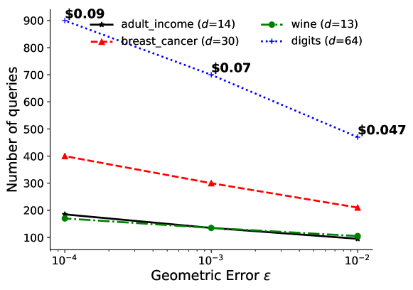
Figure 3: Number of queries needed for halfspace extraction using the version space approximation algorithm. Note that the asymptotic query complexity for this algorithm is $O(d\log\frac{1}{\varepsilon})$. This explains the increase in query complexity as a function of $d$.

Q1. Usefulness in an oracle access setting: We implemented Version Space Approximation proposed by Alabdulmohsin et al. [3] in approximately 50 lines of MATLAB. This algorithm operates iteratively, based on the principles of version space learning. A version space [51] is a hierarchical representation of knowledge. It can also be thought of as the subset of hypotheses consistent with the training examples. In each iteration, the algorithm first approximates a version space, and then synthesizes an instance that reduces this approximated version space quickly. The final query complexity for this algorithm is $O(d\log\frac{1}{\varepsilon})$.

Figure 3 plots the number of queries needed to extract a halfspace as a function of termination criterion i.e. geometric error $\varepsilon$. As discussed earlier, the query complexity is dependent on the dimensionality of the halfspace to be extracted. Across all values of dimensionality $d$, observe that with the exponential decrease in error $\varepsilon$, the increase in query complexity is linear - often by a small factor ($1.3\times-1.5\times$). The implemented query synthesis algorithm involves solving a convex optimization problem to approximate the version space, an operation that is potentially time consuming. However, based on several runs of our experiment, we noticed that the algorithm always converges in $<2$ minutes.

While the equation solving attack proposed by Tramèr et al. [67] requires fewer queries, it also requires the actual value of the prediction output i.e. $\langle w^{*},x\rangle$ as auxiliary information. On the other hand, extraction using query synthesis does not rely on any auxiliary information returned by the MLaaS server to increase its efficiency i.e. the only input needed for query synthesis-based extraction attacks is sign($\langle w^{*},x\rangle$).

Q2. Resilience to data-independent noise: An intuitive defense against model extraction might be to flip the sign of the prediction output with independent probability $\rho$ i.e. if the output $y\in\{1,-1\}$, then $Pr[y\neq\textup{sign}\langle w^{*},x\rangle]=\rho<\frac{1}{2}$ (refer subsection 5). This setting (i.e., noisy oracles) is extensively studied in the machine learning community. Trivial solutions including repeated sampling to obtain a batch where majority voting (determines the right label) can be employed; if the probability that the outcome of the vote is correct is represented as $1-\alpha$, then the batch size needed for the voting procedure is $k=O(\frac{\log\frac{1}{\alpha}}{|\rho-0.5|^{2}}$) i.e. there is an increase in query complexity by a (multiplicative) factor $k$, an expensive proposition. While other solutions exist [73, 53], we implemented the dimension coupling ($DC^{2}$) framework proposed by Chen et al. [17] in approximately 150 lines of MATLAB. The dimension coupling framework reduces a $d-$dimensional learning problem to $d-1$ lower-dimensional sub-problems. It then appropriately aggregates the results to produce a halfspace. This approach is resilient to noise i.e. the oracle can flip the label with constant probability (known a priori) $\rho<\frac{1}{2}$, and the algorithm will converge with probability $1-\delta$. The query complexity for this algorithm is $\tilde{O}(d\ (\log\frac{1}{\varepsilon}+\log\frac{1}{\delta}))$.

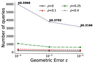
(a) Adult Income

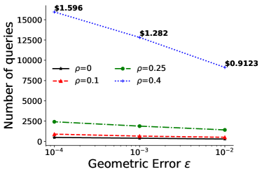
(b) Breast Cancer

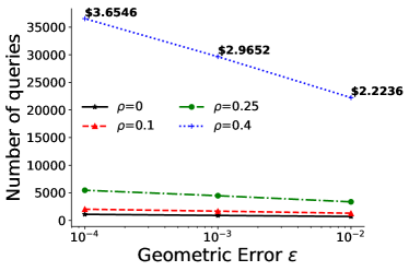
(c) Digits

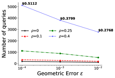
(d) Wine

Figure 4: Number of queries needed for halfspace extraction using the dimension coupling algorithm. Note that the asymptotic query complexity for this algorithm is $\tilde{O}(d(\log\frac{1}{\varepsilon}+\log\frac{1}{\delta}))$. This explains the increase in query complexity as a function of $d$.

The results of our experiment are presented in Figure 4. The algorithm is successful in extracting the halfspace for a variety of $\rho$ values. The exact bound is $C(\rho)(d\ (\log\frac{1}{\varepsilon}+\log\frac{1}{\delta})$, where $C(\rho)$ is a function of $\rho$ that is approximately $O(\frac{\rho\log^{3}(1/\rho)}{\log^{2}2(1-\rho)})$. Thus, there is a multiplicative increase in the number of queries with increase in $\rho$. This introduces a modest increase in complexity in comparison to the noise-free setting. While the increase in pricing is $\approx 40\times$, this results in a worst case expenditure of $\approx\$3.6$ (see Figure 4(c)). The time (and number of queries) taken for convergence is proportional to $\rho$, ranging from $1-20$ minutes for successful completion.

Q3. Resilience to data-dependent noise: As alluded to in subsection 5, another defense against extraction involves learning a family of functions very similar to $w^{*}$ such that they all provide accurate predictions with high probability. Proposed by Alabdulmohsin et al. [2], data-dependent randomization enables the MLaaS server to sample a random function for each query i.e. for each instance $x_{i}$, the MLaaS server obtains a new $w_{i}\thicksim\mathcal{N}(\mu,\sigma)$ and responds with $y_{i}={\textup{sign}}(\langle w_{i},x_{i}\rangle)$. Thus, this approach can be thought of as flipping the sign of the prediction output with probability $\rho_{D}(w^{*},x_{i})$ (see subsection 5).

In this algorithm, a separation parameter $C$ determines how close the samples from $\mathcal{N}(\mu,\sigma)$ are; larger the value of $C$, closer each sample is (refer Section 4 in [2] for more details). We measure the value of $\rho_{D}(w^{*},x_{i})$ as a function of $C$ for those $x_{i}$ values generated by the dimension coupling algorithm. $\rho_{D}(w^{*},x_{i})$ is estimated by (a) obtaining $w_{1},\cdots,w_{n}\thicksim\mathcal{N}(\mu,\sigma)$, for $n=1000$, and using them to classify $x_{i}$ to obtain $y_{1}=\textup{sign}(\langle w_{1},x_{i}\rangle),\cdots,y_{n}$, and (b) obtaining the percentage of the prediction outputs that is not equal to ${\textup{sign}}(\langle w^{*},x_{i}\rangle)$. Our hope was that if the value of ${\tt max}_{\forall x_{i}}~{}\rho_{D}(w^{*},x_{i})<\frac{1}{2}$, then an adversary similar to $\tilde{A}$ defined in Proposition 1 could be used to perform extraction.

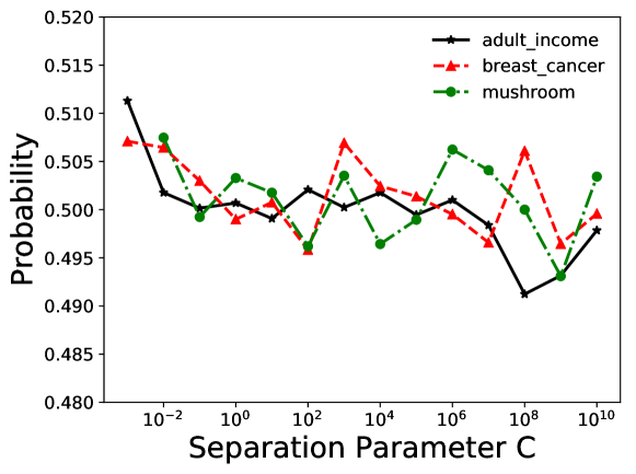
Figure 5: ${\tt average}\rho_{D}(w^{*},x_{i})\approx\frac{1}{2}\pm\gamma$; $x_{i}$ synthesized by the dimension coupling algorithm.

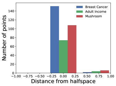
(a) Version Space Approximation

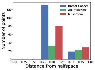
(b) $DC^{2}$

Figure 7: Distance of the instances synthesized by (a) version space approximation algorithm, and (b) dimension coupling algorithm from optimal halfspace.

Figure 5 suggests otherwise; the average value of $\rho_{D}(w^{*},x_{i})\approx\frac{1}{2}\pm\gamma$ for some small $\gamma>0$. Since any adversary will be unable to determine a priori the inputs for which this value is greater than half, neither majority voting, nor the vanilla dimension coupling framework will help extract the halfspace. We believe this is the case for current state-of-the-art algorithms as the instances they synthesize are ”close” to the optimal halfspace. To validate this claim, we measured this distance for both the algorithms [3, 17]. We observed that a majority of the points are very close to the halfspace in both cases (see Figure 7 in Appendix A.3.2 for more details).

1:Input: variance upper bound $\hat{\sigma}\geq\frac{1}{\sqrt{d}}$, target error $\varepsilon$

2:$m\leftarrow\frac{(15\pi)^{2}}{\varepsilon^{2}}d\max(1,d\hat{\sigma}^{2})\log\frac{2d}{\delta}$, $l\leftarrow\frac{1}{12d\hat{\sigma}}$

3:Draw $x_{1},x_{2},\dots,x_{m}\in\mathbb{S}^{d-1}$ uniformly at random, and query their labels $y_{1},y_{2},\dots,y_{m}$

4:$v\leftarrow\sum_{i=1}^{m}y_{i}x_{i}$

5:if $\left\|v\right\|\geq l$ then

6:     Return $w=\frac{v}{\left\|v\right\|}$

7:else

8:     Return fail

9:end if

Algorithm 1 Passive Learning Algorithm that breaks [2]

Such forms of data-dependent randomization, however, are not secure against traditional passive learning algorithms. Such an algorithm takes as input an estimated upper bound $\hat{\sigma}$ for $\sigma$. The algorithm first draws $\tilde{O}(\frac{d}{\varepsilon^{2}}\max(1,d\hat{\sigma}^{2}))$ instances from the $d-$dimensional unit sphere $\mathbb{S}^{d-1}$ uniformly at random, and proceeds to have them labeled - by the oracle defined in [2] in this case. It then computes the average $v=\sum_{i=1}^{m}y_{i}x_{i}$. $w=\frac{v}{\left\|v\right\|}$, the direction of $v$, is the algorithm’s estimate of the classifier $w^{*}$, and the length of $v$ is used as an indicator of whether the algorithm succeeds: if this estimated upper bound is correct (i.e. $\sigma\leq\hat{\sigma}$), then with high probability, $\left\|w-w^{*}\right\|\leq\varepsilon$; otherwise it outputs fail, indicating the variance bound $\hat{\sigma}$ is incorrect. In such situations, we can reduce $\hat{\sigma}$ and try again. A detailed proof of the algorithm’s guarantees is available in Appendix A.1.2.

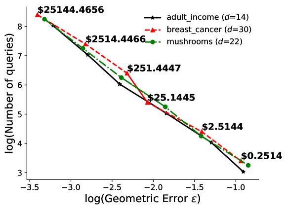
Figure 6: log(Number of queries) needed for halfspace extraction (protected by the defense strategy proposed in [2]) using Algorithm 1. Note that the asymptotic query complexity for this algorithm is $O(\frac{1}{\varepsilon^{2}}d\max(1,d\hat{\sigma}^{2})\log\frac{2d}{\delta})$. This explains the increase in query complexity as a function of $d$ and $\varepsilon$. The large value of $\frac{Cd}{\varepsilon^{2}}$ dominates the query complexity in this algorithm. The price is plotted for the attack on the breast cancer dataset.

While the asymptotic bounds for Algorithm 1 are larger than the active learning algorithms discussed thus far, the constant $\mathcal{C}=(15\pi)^{2}$ can be reduced by a multiplicative factor to reduce the total number of queries used i.e. $\frac{\mathcal{C}}{100}$ or $\frac{\mathcal{C}}{1000}$ etc. In Figure 6, we observe that extracting halfspaces with geometric error $\varepsilon\approx 10^{-1}$ requires $\leq 10^{4}$ queries. While achieving $\varepsilon\approx 10^{-3}$ requires $\approx 10^{7}$ queries, the algorithm can be executed in parallel enabling faster run-times.

Lowd and Meek Baseline: The algorithm proposed by Lowd and Meek [47] can also be used to extract a halfspace. However, note that this algorithm can only operate in a noise-free setting. This is a severe limitation if a setting where the MLaaS employs defense strategies. From Table 2, one can observe that the number of queries required to extract the halfspace is more than the query synthesis algorithms we implemented. For example, consider the breast cancer dataset. The version space algorithm is able to extract a halfspace at a distance of $\varepsilon\leq 10^{-4}$ with 400 queries (or $\$0.04$). However, the algorithm proposed by Lowd and Meek takes 970 queries for extraction. Additionally, the geometric error of the extracted halfspaces are also higher than those extracted in the query synthesis case. The query complexity of the Lowd and Meek algorithm is $O(d\log(\frac{1}{a\varepsilon}))$, where $a=\min_{i=1,\cdots,d}\frac{|w^{*}_{i}|}{\left\|w^{*}\right\|}$ ($w^{*}_{i}$ is the $i$-th coordinate of the groundtruth classifier $w^{*}$). This is worse than the $O(d\log(\frac{1}{\varepsilon}))$ query complexity of classical active learning algorithms. While this algorithm is not tailored to minimize the geometric error, we believe that these results further validate our claim that query synthesis active learning is a promising direction to explore.

Dataset	Queries	$\varepsilon$	Slowdown
Wine	189	0.071	1.67$\times$
Breast Cancer	940	0.162	3.19$\times$
Digits	1879	0.665	2.62$\times$

Table 2: Number of queries and geometric error observed after extracting halfspaces using the line search procedure proposed by Lowd and Meek. Observe that the geometric error in some cases is large. Slowdown indicates the ratio between number of queries taken for the Lowd and Meek procedure and those taken by the DC² algorithm [17] for $\varepsilon=0.01$, and $\rho=0$.

6.2 Non-Linear Models

In this section, we report experimental results for extraction efficacy for non-linear decision boundaries, specifically for kernel SVMs and decision trees. Our experiments are designed to answer the following two questions: (1) Is QS active learning practically useful to extract non-linear models (i.e., kernel SVMs) in an oracle access setting?, and (2) Is active learning useful to extract non-linear models (i.e., decision trees) in scenarios where the ML server does not reveal any auxiliary information? As before, we use the same datasets as in Tramèr et al. [67]. The continuous variables are made discrete by binning (i.e. dividing into groups), and are then one-hot-encoded. Our experiments suggest that:

1. Utilizing the extended adaptive training (EAT) approach (refer subsection 4.1) is efficient for extracting kernel SVMs. Our approach improves query complexity by 5$\times$-224$\times$.

2. Utilizing the IWAL algorithm (refer subsection 4.2) enables extracting a decision tree in the absence of any auxiliary information, with a nominal increase in query complexity (14$\times$).

Q1. Kernel SVM: As discussed in subsection 4.1, Tramèr et al. use adaptive retraining - a procedure to locate points close to the decision boundary - to obtain points used to seed their attack. Using these (labeled) points, they are able obtain the parameters which were used to instantiate the oracle using an extract-and-test approach (more specifically grid search). While techniques in active learning can not be used to expedite the grid search procedure, our experiments suggest that they are able to select more informative points i.e. points of greater uncertainty, with far fewer queries. With insight from the work of Bordes et al. [13], we propose the extended adaptive retraining approach (refer subsection 4.1) to obtain uncertain points. Additionally, we measure uncertainty with respect to a model that we train locally, eliminating redundant queries to the oracle. To compare the efficiency of our algorithm, we re-execute the adaptive retraining procedure, and present our results in Table 3.

Dataset	Adaptive Retraining		EAT
	Queries	Accuracy	Queries	Accuracy
Mushroom	11301	98.5	1001	94.5
Breast Cancer	1101	99.3	119	96.4
Adult	10901	96.98	48	98.2
Diabetes	901	98.5	166	94.8

Table 3: Extraction of a kernel SVM model. Comparison of the query complexity and test accuracy (in $\%$) obtained running Tramèr et al. adaptive retraining vs. extended adaptive retraining.

It is clear that our approach is more query efficient in comparison to Tramèr et al. (between 5$\times$-224$\times$), with comparable test accuracy. These advantages stem from (a) using a more informative metric of uncertainty than the distance from the decision boundary, and (b) querying labels of only those points which the local model is uncertain about.

Q2. Decision Trees: Tramèr et al. propose a path finding algorithm to determine the structure of the server-hosted decision tree. They rely on the server’s response to incomplete queries, and the addition of node identifiers to the generated outputs to recreate the tree. From our analysis presented in Table 1such flexibility is not readily available in most MLaaS providers. As discussed earlier (refer subsection 4.2), we utilize the IWAL algorithm proposed by Beygelzimer et al. [11] that iteratively refines a learned hypothesis. It is important to note that the IWAL algorithm is more general, and does not rely on the information needed by the path finding algorithm. We present the results of extraction using the IWAL algorithm below in Table 4.

Dataset	Oracle	Path Finding	IWAL
	Accuracy	Queries	Queries	Accuracy
Adult	81.2	18323	244188	80.2
Steak	52.1	5205	1334	73.1
Iris	86.8	246	361	89.4
GSShappiness	79	18907	254892	79.3

Table 4: Extraction of a decision tree model. Comparison of the query complexity and test accuracy (in $\%$) obtained by running path finding (Tramèr et al.) vs. IWAL algorithm. The test accuracy (in $\%$) of the server-hosted oracle is presented as a baseline.

In each iteration, the algorithm learns a new hypothesis, but the efficiency of the approach relies on the hypothesis used preceding the first iteration. To this end, we generate inputs uniformly at random. Note that in such the uniform scenario, we rely on zero auxiliary information. We can see that while the number of queries required to launch such extraction attacks is greater than in the approach proposed by Tramèr et al., such an approach obtains comparable test error to the oracle. While the authors rely on certain distributional assumptions to prove a label complexity result, we empirically observe success using the uniform strategy. Such an approach is truly powerful; it makes limited assumptions about the MLaaS provider and any prior knowledge.

7 Discussion

We begin our discussion by highlighting algorithms an adversary could use if the assumptions made about the operational ecosystem are relaxed. Then, we discuss strategies that can potentially be used to make the process of extraction more difficult, and shortcomings in our approach.

7.1 Varying The Adversary’s Capabilities

The operational ecosystem in this work is one where the adversary is able to synthesize data-points de novo to extract a model through oracle access. In this section, we discuss other algorithms an adversary could use if this assumption is relaxed. We begin by discussing other models an adversary can learn in the query synthesis regime, and move on to discussing algorithms in other approaches.

Equivalence queries. In her seminal work, Angluin [4] proposes a learning algorithm, $L^{*}$, to correctly learn a regular set from any minimally adequate teacher, in polynomial time. For this to work, however, equivalence queries are also needed along with membership queries. Should MLaaS servers provide responses to such equivalence queries, different extraction attacks could be devised. To learn linear decision boundaries, Wang et al. [71] first synthesize an instance close to the decision boundary using labeled data, and then select the real instance closest to the synthesized one as a query. Similarly, Awasthi et al. [7] study learning algorithms that make queries that are close to examples generated from the data distribution. These attacks require the adversary to have access to some subset of the original training data. In other domains, program synthesis using input-output example pairs [32, 70, 25, 58] also follows a similar principle.

If the adversary had access to a subset of the training data, or had prior knowledge of the distribution from which this data was drawn from, it could launch a different set of attacks based on the algorithms discussed below.

Stream-based selective sampling. Atlas et al. [6] propose selective sampling as a form of directed search (similar to Mitchell [50]) that can greatly increase the ability of a connectionist network (i.e. power system security analysis in their paper) to generalize accurately. Dagan et al. [20] propose a method for training probabilistic classifiers by choosing those examples from a stream that are more informative. Lindenbaum et al. [45] present a lookahead algorithm for selective sampling of examples for nearest neighbor classifiers. The algorithm looks for the example with the highest utility, taking its effect on the resulting classifier into account. Another important application of selective learning was for feature selection [46], an important preprocessing step. Other applications of stream-based selective sampling include sensor scheduling [41], learning ranking functions for information retrieval [75], and in word sense disambiguation [31].

Pool-based sampling. Dasgupta [23] surveys active learning in the non-separable case, with a special focus on statistical learning theory. He claims that in this setting, AL algorithms usually follow one of the following two strategies - (i) Efficient search in the hypothesis spaces (as in the algorithm proposed by Chen et al. [17], or by Cohn et al. [18]), or (ii) Exploiting clusters in the data (as in the algorithm proposed by Dasgupta et al. [24]). The latter option can be used to learn more complex models, such as decision trees. As the ideal halving algorithm is difficult to implement in practice, pool-based approximations are used instead such as uncertainty sampling and the query-by-committee (QBC) algorithm [30, 65, 15]. Unfortunately, such approximation methods are only guaranteed to work well if the number of unlabeled examples (i.e. pool size) grows exponentially fast with each iteration. Otherwise, such heuristics become crude approximations and they can perform quite poorly.

7.2 Complex Models

PAC active learning strategies have proven effective in learning DNNs. The work of Sener et al. [60] selects the most representative points from a sample of the training distribution to learn the DNN. Papernot et al. [55] employ substitute model training - a procedure where a small training subset is strategically augmented and used to train a shadow model that resembles the model being attacked. Note that the prior approaches rely on some additional information, such as a subset of the training data.

Active learning algorithms considered in this paper work in an iterative fashion. Let $\mathcal{H}$ be the entire hypothesis class. At time time $t\geq 0$ let the set of possible hypothesis be $\mathcal{H}_{t}\subseteq\mathcal{H}$. Usually an active-learning algorithm issues a query at time $t$ and updates the possible set of hypothesis to $\mathcal{H}_{t+1}$, which is a subset of $\mathcal{H}_{t}$. Once the size of $\mathcal{H}_{t}$ is “small” the algorithm stops. Analyzing the effect of a query on possible set of hypothesis is very complicated in the context of complex models, such as DNNs. We believe this is a very important and interesting direction for future work.

7.3 Model Transferability

Most work in active learning has assumed that the correct hypothesis space for the task is already known i.e. if the model being learned is for logistic regression, or is a neural network and so on. In such situations, observe that the labeled data being used is biased, in that it is implicitly tied to the underlying hypothesis. Thus, it can become problematic if one wishes to re-use the labeled data chosen to learn another, different hypothesis space. This leads us to model transferability, a less studied form of defense where the oracle responds to any query with the prediction output from an entirely different hypothesis class. For example, imagine if a learner tries to learn a halfspace, but the teacher performs prediction using a boolean decision tree. Initial work in this space includes that of Shi et al. [62], where an adversary can steal a linear separator by learning input-output relations using a deep neural network. However, the performance of query synthesis active learning in such ecosystems is unclear.

7.4 Limitations

We stress that these limitations are not a function of our specific approach, and stem from the theory of active learning. Specifically: (1) As noted by Dasgupta [22], the label complexity of PAC active learning depends heavily on the specific target hypothesis, and can range from $O(\log\frac{1}{\varepsilon})$ to $\Omega(\frac{1}{\varepsilon})$. Similar results have been obtained by others [35, 52]. This suggests that for some hypotheses classes, the query complexity of active learning algorithms is as high as that in the passive setting. (2) Some query synthesis algorithms assume that there is some labeled data to bootstrap the system. However, this may not always be true, and randomly generating these labeled points may adversely impact the performance of the algorithm. (3) For our particular implementation, the algorithms proposed rely on the geometric error between the optimal and learned halfspaces. Oftentimes, however, there is no direct correlation between this geometric error and the generalization error used to measure the model’s goodness.

8 Related Work

Machine learning algorithms and systems are optimized for performance. Little attention is paid to the security and privacy risks of these systems and algorithms. Our work is motivated by the following attacks against machine learning.

1. Causative Attacks: These attacks are primarily geared at poisoning the training data used for learning, such that the classifier produced performs erroneously during test time. These include: (a) mislabeling the training data, (b) changing rewards in the case of reinforcement learning, or (c) modifying the sampling mechanism (to add some bias) such that it does not reflect the true underlying distribution in the case of unsupervised learning [57]. The work of Papernot et al. [56] modify input features resulting in misclassification by Deep Neural Networks.

2. Evasion Attacks: Once the algorithm has trained successfully, these forms of attacks provide tailored inputs such that the output is erroneous. These noisy inputs often preserves the semantics of the original inputs, are human imperceptible, or are physically realizable. The well studied area of adversarial examples is an instantiation of such an attack. Moreover, evasion attacks can also be even black-box i.e. the attacker needn’t know the model. This is because an adversarial example optimized for one model is highly likely to be effective for other models. This concept, known as transferability, was introduced by Carlini et al. [16]. Notable works in this space include [12, 26, 42, 43, 66, 55, 72, 28]

3. Exploratory Attacks: These forms of attacks are the primary focus of this work, and are geared at learning intrinsics about the algorithm used for training. These intrinsics can include learning model parameters, hyperparameters, or training data. Typically, these forms of attacks fall in two categories - model inversion, or model extraction. In the first class, Fredrikson et al. [29] show that an attacker can learn sensitive information about the dataset used to train a model, given access to side-channel information about the dataset. In the second class, the work of Tramer et al. [67] provides attacks to learn parameters of a model hosted on the cloud, through a query interface. Termed membership inference, Shokri et al. [63] learn the training data used for machine learning by training their own inference models. Wang et al. [69] propose attacks to learn a model’s hyperparameters.

9 Conclusions

In this paper, we formalize model extraction in the context of Machine-Learning-as-a-Service (MLaaS) servers that return only prediction values (i.e., oracle access setting), and we study its relation with query synthesis active learning (Observation 1). Thus, we are able to implement efficient attacks to the class of halfspace models used for binary classification (Section 6). While our experiments focus on the class of halfspace models, we believe that extraction via active learning can be extended to multiclass and non-linear models such as deep neural networks, random forests etc. We also begin exploring possible defense approaches (subsection 5). To the best of our knowledge, this is the first work to formalize security in the context of MLaaS systems. We believe this is a fundamental first step in designing more secure MLaaS systems. Finally, we suggest that data-dependent randomization (e.g., model randomization as in [2]) is the most promising direction to follow in order to design effective defenses.

10 Acknowledgements

This material is partially supported by Air Force Grant FA9550-18-1-0166, the National Science Foundation (NSF) Grants CCF-FMitF-1836978, SaTC-Frontiers-1804648 and CCF-1652140 and ARO grant number W911NF-17-1-0405. Kamalika Chaudhuri and Songbai Yan thank NSF under 1719133 and 1804829 for research support.

Appendix A Appendix

A.1 Proofs

A.1.1 Proof of Proposition 1

Proof.

Let $\tilde{\mathcal{A}}$ be the adversary that does the following:

for $i=1,\dots,q(\varepsilon,\delta)$

1. $\tilde{A}$ uses the query strategy of $\mathcal{L}$ to generate the instance $x_{i}$;

2. $\tilde{A}$ queries $x_{i}$ to $S_{D}(f^{*})$ for $r$ times and defines $y_{i}$ the most frequent labels among the $r$ answers (we assume $r$ is an even integer).

At the end, $\tilde{A}$ (as the learner $\mathcal{L}$) learns $\hat{f}$ using the points $\{(x_{i},y_{i})\}_{i=1,\cdots,q(\varepsilon,\delta)}$. Let $q=r\cdot q(\varepsilon,\delta)$, then it holds by the union bound that

$$\Pr[\textup{{Exp}}^{\varepsilon}_{\mathcal{F}}(S_{D}(f^{*}),\tilde{A},q)=1]\geq$$

$$1-\delta-(1-\Pr[\cap_{i=1}^{q(\varepsilon,\delta)}\{y_{i}=f^{*}(x_{i})\}])\,.$$

Define $X_{i}^{j}$ as the binary random variable that is 1 if and only if the answer to the $j$-th query of $x_{i}$ is correct and $X_{i}=\sum_{j=1}^{r}X_{i}^{j}$, then

$$\Pr[\cap_{i=1}^{q(\varepsilon,\delta)}\{y_{i}=f^{*}(x_{i})\}] \geq\Pr[\cap_{i=1}^{q(\varepsilon,\delta)}\{X_{i}>r/2\}]$$

$$\geq 1-\sum_{i=1}^{q(\varepsilon,\delta)}\Pr[\{X_{i}\leq r/2\}]$$

where the last step follows from the union bound. Now, observe that $\mathbb{E}[X_{i}]=r(1-\rho_{D}(f^{*},x_{i}))>r/2$ and the Chernoff bound can be applied on each term in the right-hand side. In particular, we have that $\Pr[\{X_{i}\leq r/2\}]\leq e^{-r\frac{\left(\rho_{D}(f^{*})-\frac{1}{2}\right)^{2}}{2}}$ and it follows that

$$\Pr[\textup{{Exp}}^{\varepsilon}_{\mathcal{F}}(S_{D}(f^{*}),\tilde{A},q)=1]\geq 1-\delta-q(\varepsilon,\delta)\,e^{-r\frac{(\rho_{D}(f^{*})-\frac{1}{2})^{2}}{2}}\,.$$

By setting $r=\frac{8}{(1-2\rho_{D}(f^{*}))^{2}}\ln\frac{q(\varepsilon,\delta)}{\delta}$ we have $\Pr[\textup{{Exp}}^{\varepsilon}_{\mathcal{F}}(S_{D}(f^{*}),\tilde{A},q)=1]\geq 1-2\delta$. That is, the adversary $\tilde{A}$ implements an $\varepsilon$-extraction with Confidence Score $1-2\delta$ and complexity $q=\frac{8}{(1-2\rho_{D}(f^{*}))^{2}}q(\varepsilon,\delta)\ln\frac{q(\varepsilon,\delta)}{\delta}$.
∎

A.1.2 Proof of Algorithm 1

Here, we discuss the analysis and proofs associated with Algorithm 1.

Assume unit vector $\mu\in\mathbb{R}^{d}$ is the ground truth. For each query $x\in\mathbb{R}^{d}$, a vector $w$ is drawn from $N(\mu,\sigma^{2}I)$, and the label $y=\text{sign}(\left\langle w,x\right\rangle)$ is returned. The goal of the learner (attacker) is to return $\hat{w}$ such that $\left\|\mu-\hat{w}\right\|$ is small.

We have following theoretical guarantees for Algorithm 1.

Proposition 1.

If $\sigma\leq\hat{\sigma}$, then $\left\|\hat{w}-\mu\right\|\leq\varepsilon$ with probability at least $1-\delta$.

Proposition 2.

If $\sigma\leq\hat{\sigma}$ and $\hat{\sigma}\geq\frac{1}{\sqrt{d}}$, then $\left\|v\right\|\geq\frac{1}{12d\hat{\sigma}}$ with probability at least $1-\delta$.

Proposition 3.

If $\sigma\geq 20\hat{\sigma}\geq\frac{1}{\sqrt{d}}$, then $\left\|v\right\|\leq\frac{1}{\sqrt{148}d\hat{\sigma}}$ with probability at least $1-\delta$.

Propositions 1 and 2 guarantees that if the estimated upper bound is correct ($\sigma\leq\hat{\sigma}$), then the algorithm outputs an accurate estimation of $\mu$; Proposition 3 guarantees the algorithm declares failure if the estimated upper bound is too small ($\hat{\sigma}\leq\frac{1}{20}\sigma$).

Intuitively, the average of $y_{i}x_{i}$ ($i=1,\dots,m$) points to a direction similar to $\mu$ because of the symmetry of distributions of both $x$ and noise: the projection of $yx$ onto all directions perpendicular to $\mu$ is distributed symmetrically around 0 and thus has mean 0. The projection of $yx$ onto $\mu$ has non-negative mean since the label $y$ is correct (i.e., $yv^{\top}x\geq 0$) with probability at least $\frac{1}{2}$, and the projection is larger if the noise of $y$ is smaller. Consequently, the scale of the average can be used as an indicator of the noise level. The Propositions can be formally proved by applying concentration inequalities on each direction.

Notation.

Denote by $\mathbb{S}^{d-1}$ the unit sphere $\{x\in\mathbb{R}^{d}:x^{\top}x=1\}$. For any vector $X\in\mathbb{R}^{d}$, denote by $X^{(i)}$ the $i$-th coordinate of $X$. Define $Z_{i}=Y_{i}X_{i}$ for $i=1,2,\dots,m$.

We need following facts.

Fact 1.

$\Pr(w^{\top}x\geq 0)=\Pr_{\xi\sim N(0,1)}(\xi\geq-\frac{w^{\star\top}x}{\sigma\left\|x\right\|})$. Moreover, for $z\geq 0$, $\frac{1}{2}-\frac{z}{\sqrt{2\pi}\sigma}\leq\Pr_{\xi\sim N(0,1)}(\xi\geq\frac{z}{\sigma})\leq\max(\frac{1}{6},\frac{1}{2}-\frac{z}{3\sigma})$.

Fact 2.

Let $B(x,y)=\int_{0}^{1}(1-t)^{x-1}t^{y-1}dt$ be the Beta function. Then $\frac{2}{\sqrt{d-1}}\leq B(\frac{1}{2},\frac{d}{2})\leq\frac{\pi}{\sqrt{d}}$.

Fact 3.

If $d\geq 2$, then $(1-\frac{1}{d})^{\frac{d}{2}}\geq\frac{1}{2}$.

Fact 4.

(Bernstein inequality) If i.i.d. random variables $X_{1},\dots,X_{m}$ satisfy $|X_{i}|\leq b$, $\mathbb{E}[X_{i}]=\mu$, and $\mathbb{E}[X_{i}^{2}]\leq r^{2}$, then with probability at least $1-\delta$, $|\frac{1}{m}\sum_{i=1}^{m}X_{i}-\mu|\leq\sqrt{\frac{2r^{2}}{m}\log\frac{2}{\delta}}+\frac{2b}{3m}\log\frac{2}{\delta}$.

Fact 5.

Suppose $(x_{1},\dots,x_{d})$ is drawn from the uniform distribution over the unit sphere, then $x_{1}$ has a density function of $p(z)=\frac{(1-z^{2})^{\frac{d-3}{2}}}{B(\frac{d-1}{2},\frac{1}{2})}$.

Without loss of generality, assume $\mu=(1,0,0,\dots,0)$.

Following three lemmas give concentration of $v$.

Lemma 1.

For any $k=2,3,\dots,d$, with probability at least $1-\delta$, $|v^{(k)}|\leq 2\sqrt{\frac{2}{md}\log\frac{2}{\delta}}$.

Proof.

For $k=2,3,\dots,d$, $Z_{1}^{(k)},Z_{2}^{(k)},\dots,Z_{m}^{(k)}$ are i.i.d. random variables bounded by 1. By symmetry, $\mathbb{E}[Z_{1}^{(k)}]=0$. $\mathbb{E}[(Z_{1}^{(k)})^{2}]=\mathbb{E}[(X^{(i)})^{2}]=2\int_{0}^{1}z^{2}\frac{(1-z^{2})^{\frac{d-3}{2}}}{B(\frac{d-1}{2},\frac{1}{2})}dz=\frac{1}{B(\frac{d-1}{2},\frac{1}{2})}\int_{0}^{1}t^{\frac{1}{2}}(1-t)^{\frac{d-3}{2}}dt=\frac{B(\frac{d-1}{2},\frac{3}{2})}{B(\frac{d-1}{2},\frac{1}{2})}=\frac{1}{d}$. By the Bernstein inequality, with probability at least $1-\delta$, $|\frac{1}{m}\sum Z_{i}^{(k)}|\leq\sqrt{\frac{2}{md}\log\frac{2}{\delta}}+\frac{2}{3m}\log\frac{2}{\delta}\leq 2\sqrt{\frac{2}{md}\log\frac{2}{\delta}}$. ∎

Lemma 2.

With probability at least $1-\delta$, $v^{(1)}\geq\frac{1}{3\pi\sqrt{d}}\min(1,\frac{1}{\sigma\sqrt{d}})-\sqrt{\frac{1}{2m}\log\frac{1}{\delta}}$.

Proof.

$Z_{1}^{(1)},Z_{2}^{(1)},\dots,Z_{m}^{(1)}$ are i.i.d. random variables bounded by 1. Their mean can be lower-bounded as follows.

For for any $0\leq a\leq 1$, due to the noise setting, $\mathbb{E}[Y\mid X^{(1)}=a]\geq 0$ and $\mathbb{E}[Y\mid X^{(1)}=-a]\leq 0$, so $\mathbb{E}[YX^{(1)}\mid X^{(1)}=a]+\mathbb{E}[YX^{(1)}\mid X^{(1)}=-a]\geq 0$. Consequently we have

$$\mathbb{E}[YX^{(1)}] \geq\mathbb{E}[YX^{(1)}\mathds{1}[|X^{(1)}|\geq\frac{1}{\sqrt{d}}]]$$

$$=\mathbb{E}[\mathbb{E}[Y\mid X^{(1)}]X^{(1)}\mathds{1}[|X^{(1)}|\geq\frac{1}{\sqrt{d}}]]$$

$$=\mathbb{E}[(1-2\Pr[Y=-1\mid X^{(1)}])X^{(1)}\mathds{1}[X^{(1)}\geq\frac{1}{\sqrt{d}}]]$$

$$\geq(1-2\Pr_{\xi\sim N(0,1)}(\xi\geq\frac{1}{\sigma\sqrt{d}}))\mathbb{E}[X^{(1)}\mathds{1}[X^{(1)}\geq\frac{1}{\sqrt{d}}]]$$

Now, $\Pr_{\xi\sim N(0,1)}(\xi\geq\frac{1}{\sigma\sqrt{d}})\leq\max(\frac{1}{6},\frac{1}{2}-\frac{1}{3\sigma\sqrt{d}})$. Besides, $\mathbb{E}[X^{(1)}\mathds{1}[X^{(1)}\geq\frac{1}{\sqrt{d}}]]=\int_{\frac{1}{\sqrt{d}}}^{1}\frac{z(1-z^{2})^{\frac{d-3}{2}}}{B(\frac{d-1}{2},\frac{1}{2})}dz=\frac{(1-\frac{1}{d})^{\frac{d-1}{2}}}{(d-1)B(\frac{d-1}{2},\frac{1}{2})}\geq\frac{1}{2(d-1)\frac{\pi}{\sqrt{d-1}}}\geq\frac{1}{2\pi\sqrt{d}}$ where the first inequality follows by Fact 2 and 3. Thus, $\mathbb{E}[YX^{(1)}]\geq\frac{1}{3\pi\sqrt{d}}\min(1,\frac{1}{\sigma\sqrt{d}})$.

By the Chernoff bound, with probability at least $1-\delta$, $v^{(1)}=\frac{1}{m}\sum Z_{i}^{(1)}\geq\frac{1}{3\pi\sqrt{d}}\min(1,\frac{1}{\sigma\sqrt{d}})-\sqrt{\frac{1}{2m}\log\frac{1}{\delta}}$. ∎

Lemma 3.

With probability at least $1-\delta$, $v^{(1)}\leq\frac{2}{\sqrt{2\pi}d\sigma}+\sqrt{\frac{1}{2m}\log\frac{1}{\delta}}$.

Proof.

We first give an upper bound of $\mathbb{E}[YX^{(1)}]=2\int_{0}^{1}z\frac{(1-z^{2})^{\frac{d-3}{2}}}{B(\frac{d-1}{2},\frac{1}{2})}(1-2\Pr_{\xi\sim N(0,1)}(\xi\geq\frac{z}{\sigma}))dz$. By Fact 1, $1-2\Pr_{\xi\sim N(0,1)}(\xi\geq\frac{z}{\sigma})\leq\frac{2z}{\sqrt{2\pi}\sigma}$, so we have

$$\mathbb{E}[YX^{(1)}] \leq 2\int_{0}^{1}z\frac{(1-z^{2})^{\frac{d-3}{2}}}{B(\frac{d-1}{2},\frac{1}{2})}\frac{2z}{\sqrt{2\pi}\sigma}dz$$

$$=\frac{4}{\sqrt{2\pi}\sigma B(\frac{d-1}{2},\frac{1}{2})}\int_{0}^{1}z^{2}(1-z^{2})^{\frac{d-3}{2}}dz$$

$$=\frac{2B(\frac{d-1}{2},\frac{3}{2})}{\sqrt{2\pi}\sigma B(\frac{d-1}{2},\frac{1}{2})}$$

$$=\frac{2}{\sqrt{2\pi}d\sigma}$$

The conclusion follows by the Chernoff bound. ∎

Now we present the proofs for the propositions.

Proof.

(of Proposition 1) Since $\left\|\hat{w}-\mu\right\|^{2}=\left\|\hat{w}\right\|^{2}+\left\|\mu\right\|^{2}-2\mu^{\top}\hat{w}=2(1-\mu^{\top}\hat{w})=2(1-\frac{v^{(1)}}{\left\|v\right\|})$, to prove $\left\|\hat{w}-\mu\right\|\leq\varepsilon$, it suffices to show $\frac{v^{(1)}}{\left\|v\right\|}\geq 1-\frac{\varepsilon^{2}}{2}$. Note that $1-(\frac{v^{(1)}}{\left\|v\right\|})^{2}=\frac{1}{1+\frac{(v^{(1)})^{2}}{\sum_{k=2}^{d}(v^{(k)})^{2}}}$, and $1-(1-\frac{\varepsilon^{2}}{2})^{2}=\varepsilon^{2}-\frac{\varepsilon^{4}}{4}\geq\frac{\varepsilon^{2}}{2}\geq\frac{1}{1+\frac{2}{\varepsilon^{2}}}$ , so it suffices to show $\frac{(v^{(1)})^{2}}{\sum_{k=2}^{d}(v^{(k)})^{2}}\geq\frac{2}{\varepsilon^{2}}$ with probability at least $1-\delta$.

Now, by Lemma 1 and 2 and a union bound, with probability at least $1-\delta$,

$$\frac{(v^{(1)})^{2}}{\sum_{k=2}^{d}(v^{(k)})^{2}}\geq\frac{(\frac{1}{3\pi\sqrt{d}}\min(1,\frac{1}{\sigma\sqrt{d}})-\sqrt{\frac{1}{2m}\log\frac{d}{\delta}})^{2}}{4(d-1)\frac{2}{md}\log\frac{2d}{\delta}},$$

which is at least $\frac{2}{\varepsilon^{2}}$ for our setting of $m=\frac{(15\pi)^{2}}{\varepsilon^{2}}d\max(1,d\hat{\sigma}^{2})\log\frac{2d}{\delta}$. ∎

Proof.

(of Proposition 2) By Lemma 2, with probability at least $1-\delta$, $v^{(1)}=\frac{1}{m}\sum Z_{i}^{(1)}\geq\frac{1}{3\pi\sqrt{d}}\min(1,\frac{1}{\sigma\sqrt{d}})-\sqrt{\frac{1}{2m}\log\frac{1}{\delta}}\geq\frac{1}{12\sqrt{d}}\min(1,\frac{1}{\hat{\sigma}\sqrt{d}})$, which implies $\left\|v\right\|\geq v^{(1)}\geq\frac{1}{12\sqrt{d}}\min(1,\frac{1}{\hat{\sigma}\sqrt{d}})$. ∎

Proof.

(of Proposition 3) By Lemma 1 and 3 and a union bound, with probability at least $1-\delta$,

$$\left\|v\right\|^{2} =\sum_{k=1}^{d}(v^{(k)})^{2}$$

$$\leq 4(d-1)\frac{2}{md}\log\frac{2d}{\delta}+(\frac{2}{\sqrt{2\pi}d\sigma}+\sqrt{\frac{1}{2m}\log\frac{1}{\delta}})^{2}$$

$$\leq\frac{1}{148d^{2}\hat{\sigma}^{2}}.$$

∎

A.2 Noisy Labels for the Continuous Case

In the continuous, the model extraction problem becomes a regression problem. In [19] the authors consider passive linear regression with squared loss and provide an algorithm that achieves nearly optimal convergence rate $\mathbb{E}[X^{\top}\hat{w}-Y]-\mathbb{E}[X^{\top}w^{\star}-Y]=\tilde{O}\left(\frac{C}{n}\right)$ where the constant $C$ depends on the covariance matrix of $X$ and the error of the optimal linear model $w^{\star}$. In [59] the authors point out that unlike in the classification case, the $O(\frac{1}{n})$ cannot be improved by active learning, but it provides an algorithm under a stream-based querying model (in fact, they assume the algorithm can draw $X$ from any distribution, which can be implemented by rejection sampling with stream-based querying model) that achieves a learning rate with a better constant factor $C$. Authors in [27] consider active learning for maximum likelihood estimation (MLE) under the assumption that the model is well-specified ($P(Y|X)$ is given by a model in the model class) and that the Fisher information matrix does not depend on label $y$ (this assumption holds for linear regression and generalized linear models). It shows that a two-stage algorithm achieves a nearly optimal convergence rate.

The main difficulties of computationally efficient active learning for classification arise because of two factors: (1) how to efficiently find a classifier with the minimum classification error rate; (2) how to select examples for labeling. For (1), it has been shown that optimizing the classification error rate (0-1 loss) with noise is hard in general, and computational efficient solutions with theoretical guarantees are only known under some assumptions of the hypothesis space and noise conditions (for example [17, 40, 74]). For (2), most existing active learning algorithms maintain a candidate set of classifiers either explicitly [33] or implicitly [17, 21, 74], and the noise tolerance is achieved by repetitive querying as in Proposition 1 or a carefully designed sampling schedule to guarantee that the candidate set is “correctly shrunk” with high probability [21, 33, 74]. For regression, most loss functions (for example the squared error, negative log likelihood) are convex, and thus can be optimized efficiently. The labeling strategies in regression are also different: instead of maintaining candidate sets, active regression algorithms [59, 27] often first find a good sampling distribution that optimize some statistics of the covariance matrix and then draw labeled samples from this distribution. Such strategies tolerates noise naturally and de-noising strategies like repetitive querying are not necessary.

A.3 Additional Results

A.3.1 Alternate Stopping Criterion

We investigated if measuring the model’s stability over $N$ iterations results in acceptable extraction attacks. Here, we define model stability as the oscillation between the approximation learned at iteration $i$ and at iteration $i+1$. Formally, stability can be defined as $\mathcal{S}_{i}=||w_{i}-w_{i+1}||_{2}$. Our approach checks if $\mathcal{S}_{i}\leq\tau$ for $i=1,\cdots,N$ and terminates execution if the condition is satisfied. We observe that this approach fails for the algorithm proposed by Chen et al. [17], as the approximation produced at each iteration differs greatly from the approximation produced in the preceding iteration. The results for the algorithm proposed by Alabdulmohsin et al. [3] can be found Table 5.

	N=10		N=15		N=20		Baseline
Dataset	Queries	$\hat{\varepsilon}$	Queries	$\hat{\varepsilon}$	Queries	$\hat{\varepsilon}$	$\varepsilon=0.001$
Breast Cancer	241	0.0047	247	0.0034	252	0.0031	300
Adult Income	117	0.0019	122	0.0015	127	0.0012	135
Digits	493	0.0077	498	0.0075	503	0.0073	700
Wine	120	0.0016	125	0.0014	130	0.0012	135

Table 5: Model stability results in nominal savings at the expense of a small increase in geometric error ($\hat{\varepsilon}$). The trends are the same for other values of $\varepsilon$.

A.3.2 A Direction For Defense?

Recall from earlier discussion that QS active learning algorithms are capable of generating points de novo. It is conceivable that these points are not generated from the distribution from which the training data is sampled from. To this end, we verified if these distributions are indeed different using the Hotelling’s $T^{2}$ test, specifically for the algorithms proposed by Alabdulmohsin et al. [3] and Chen et al. [17] under the null hypothesis that the distributions are the same (refer Table 6 and Table 7). We observe that this QS active learning algorithm indeed produces points that are not from the underlying natural distribution. While discarding points that can not be sampled from the training distribution may seem as a tempting defense strategy, it is conceivable that certain real world tasks may query MLaaS providers with outlier points. Further analysis is required to determine how this strategy may effectively be used to defend against model extraction.

Dataset	t-value	n-1	p-value	Reject Null?
Breast Cancer	14.24	198	3.70 $\times$ 10 -32	✓
Adult Income	9.71	92	9.22 $\times$ 10 -16	✓
Mushroom	22.16	599	5.92 $\times$ 10 -80	✓

Table 6: Results of the Hotelling $T^{2}$ test for multivariate distributions, for n samples. It is observed that the data-points generated by the version space approximation algorithm do not lie in the natural distribution underlined by samples from the training data.

Dataset	t-value	n-1	p-value	Reject Null?
Breast Cancer	319.27	322	0	✓
Adult Income	467.43	133	9.64 $\times$ 10 -216	✓
Mushroom	65.74	222	1.58 $\times$ 10 -147	✓

Table 7: Results of the Hotelling $T^{2}$ test for multivariate distributions, for n samples. It is observed that the data-points generated by the DC² algorithm do not lie in the natural distribution underlined by samples from the training data.

References

- [1] https://archive.ics.uci.edu/ml/datasets.html, 2018.
- [2] Ibrahim M. Alabdulmohsin, Xin Gao, and Xiangliang Zhang. Adding robustness to support vector machines against adversarial reverse engineering. In Proceedings of the 23rd ACM International Conference on Conference on Information and Knowledge Management, CIKM 2014, Shanghai, China, November 3-7, 2014, pages 231–240, 2014.
- [3] Ibrahim M Alabdulmohsin, Xin Gao, and Xiangliang Zhang. Efficient active learning of halfspaces via query synthesis. In AAAI, pages 2483–2489, 2015.
- [4] Dana Angluin. Learning regular sets from queries and counterexamples. Information and computation, 75(2):87–106, 1987.
- [5] Giuseppe Ateniese, Luigi V. Mancini, Angelo Spognardi, Antonio Villani, Domenico Vitali, and Giovanni Felici. Hacking smart machines with smarter ones: How to extract meaningful data from machine learning classifiers. IJSN, 10(3):137–150, 2015.
- [6] Les E Atlas, David A Cohn, and Richard E Ladner. Training connectionist networks with queries and selective sampling. In Advances in neural information processing systems, pages 566–573, 1990.
- [7] Pranjal Awasthi, Vitaly Feldman, and Varun Kanade. Learning using local membership queries. In Conference on Learning Theory, pages 398–431, 2013.
- [8] Maria-Florina Balcan, Alina Beygelzimer, and John Langford. Agnostic active learning. Journal of Computer and System Sciences, 75(1):78–89, 2009.
- [9] Maria-Florina Balcan, Andrei Z. Broder, and Tong Zhang. Margin based active learning. In Learning Theory, 20th Annual Conference on Learning Theory, COLT 2007, San Diego, CA, USA, June 13-15, 2007, Proceedings, pages 35–50, 2007.
- [10] Maria-Florina Balcan and Philip M. Long. Active and passive learning of linear separators under log-concave distributions. In COLT 2013 - The 26th Annual Conference on Learning Theory, June 12-14, 2013, Princeton University, NJ, USA, pages 288–316, 2013.
- [11] Alina Beygelzimer, Daniel Hsu, John Langford, and Tong Zhang. Agnostic active learning without constraints. In 23rd International Conference on Neural Information Processing Systems (NIPS), 2010.
- [12] Arjun Nitin Bhagoji, Warren He, Bo Li, and Dawn Song. Black-box attacks on deep neural networks via gradient estimation. 2018.
- [13] Antoine Bordes, Seyda Ertekin, Jason Weston, and Leon Bottou. Fast kernel classifiers with online and active learning. Journal of Machine Learning Research (JMLR), September 2005.
- [14] Wieland Brendel, Jonas Rauber, and Matthias Bethge. Decision-based adversarial attacks: Reliable attacks against black-box machine learning models. arXiv preprint arXiv:1712.04248, 2017.
- [15] Klaus Brinker. Incorporating diversity in active learning with support vector machines. In Proceedings of the 20th International Conference on Machine Learning (ICML-03), pages 59–66, 2003.
- [16] Nicholas Carlini and David Wagner. Towards evaluating the robustness of neural networks. In Security and Privacy (SP), 2017 IEEE Symposium on, pages 39–57. IEEE, 2017.
- [17] Lin Chen, Seyed Hamed Hassani, and Amin Karbasi. Near-optimal active learning of halfspaces via query synthesis in the noisy setting. In AAAI, pages 1798–1804, 2017.
- [18] David Cohn, Les Atlas, and Richard Ladner. Improving generalization with active learning. Machine learning, 15(2):201–221, 1994.
- [19] Hsu D. and Sabato S. Heavy-tailed regression with a generalized median-of-means. In International Conference on Machine Learning (ICML), 2014.
- [20] Ido Dagan and Sean P Engelson. Committee-based sampling for training probabilistic classifiers. In Proceedings of the Twelfth International Conference on Machine Learning, pages 150–157. The Morgan Kaufmann series in machine learning,(San Francisco, CA, USA), 1995.
- [21] S. Dasgupta, D. Hsu, and C. Monteleoni. A general agnostic active learning algorithm. In NIPS, 2007.
- [22] Sanjoy Dasgupta. Coarse sample complexity bounds for active learning. In Advances in Neural Information Processing Systems 18 [Neural Information Processing Systems, NIPS 2005, December 5-8, 2005, Vancouver, British Columbia, Canada], pages 235–242, 2005.
- [23] Sanjoy Dasgupta. Two faces of active learning. Theoretical computer science, 412(19):1767–1781, 2011.
- [24] Sanjoy Dasgupta, Daniel J Hsu, and Claire Monteleoni. A general agnostic active learning algorithm. In Advances in neural information processing systems, pages 353–360, 2008.
- [25] Dana Drachsler-Cohen, Sharon Shoham, and Eran Yahav. Synthesis with abstract examples. In International Conference on Computer Aided Verification, pages 254–278. Springer, 2017.
- [26] Gamaleldin F Elsayed, Shreya Shankar, Brian Cheung, Nicolas Papernot, Alex Kurakin, Ian Goodfellow, and Jascha Sohl-Dickstein. Adversarial examples that fool both human and computer vision. arXiv preprint arXiv:1802.08195, 2018.
- [27] Chaudhuri K. et al. Convergence rates of active learning for maximum likelihood estimation. In Advances in Neural Information Processing Systems, 2015.
- [28] Ivan Evtimov, Kevin Eykholt, Earlence Fernandes, Tadayoshi Kohno, Bo Li, Atul Prakash, Amir Rahmati, and Dawn Song. Robust physical-world attacks on deep learning models. arXiv preprint arXiv:1707.08945, 1, 2017.
- [29] Matthew Fredrikson, Eric Lantz, Somesh Jha, Simon Lin, David Page, and Thomas Ristenpart. Privacy in pharmacogenetics: An end-to-end case study of personalized warfarin dosing. In USENIX Security Symposium, pages 17–32, 2014.
- [30] Yoav Freund, H Sebastian Seung, Eli Shamir, and Naftali Tishby. Selective sampling using the query by committee algorithm. Machine learning, 28(2):133–168, 1997.
- [31] Atsushi Fujii, Takenobu Tokunaga, Kentaro Inui, and Hozumi Tanaka. Selective sampling for example-based word sense disambiguation. Computational Linguistics, 24(4):573–597, 1998.
- [32] Sumit Gulwani. Synthesis from examples: Interaction models and algorithms. In Symbolic and Numeric Algorithms for Scientific Computing (SYNASC), 2012 14th International Symposium on, pages 8–14. IEEE, 2012.
- [33] S. Hanneke. A bound on the label complexity of agnostic active learning. In ICML, 2007.
- [34] Steve Hanneke. Theory of disagreement-based active learning. Foundations and Trends in Machine Learning, 7(2-3):131–309, 2014.
- [35] Tibor Hegedűs. Generalized teaching dimensions and the query complexity of learning. In Proceedings of the eighth annual conference on Computational learning theory, pages 108–117. ACM, 1995.
- [36] Ling Huang, Anthony D. Joseph, Blaine Nelson, Benjamin I. P. Rubinstein, and J. D. Tygar. Adversarial machine learning. In Proceedings of the 4th ACM Workshop on Security and Artificial Intelligence, AISec 2011, Chicago, IL, USA, October 21, 2011, pages 43–58, 2011.
- [37] Matti Kääriäinen. Active learning in the non-realizable case. In Algorithmic Learning Theory, 17th International Conference, ALT 2006, Barcelona, Spain, October 7-10, 2006, Proceedings, pages 63–77, 2006.
- [38] Richard M. Karp and Robert Kleinberg. Noisy binary search and its applications. In Proceedings of the Eighteenth Annual ACM-SIAM Symposium on Discrete Algorithms, SODA 2007, New Orleans, Louisiana, USA, January 7-9, 2007, pages 881–890, 2007.
- [39] Ross D King, Jem Rowland, Stephen G Oliver, Michael Young, Wayne Aubrey, Emma Byrne, Maria Liakata, Magdalena Markham, Pinar Pir, Larisa N Soldatova, et al. The automation of science. Science, 324(5923):85–89, 2009.
- [40] Adam R. Klivans and Pravesh Kothari. Embedding hard learning problems into gaussian space. In Approximation, Randomization, and Combinatorial Optimization. Algorithms and Techniques, APPROX/RANDOM 2014, September 4-6, 2014, Barcelona, Spain, pages 793–809, 2014.
- [41] Vikram Krishnamurthy. Algorithms for optimal scheduling and management of hidden markov model sensors. IEEE Transactions on Signal Processing, 50(6):1382–1397, 2002.
- [42] Alex Kurakin, Dan Boneh, Florian Tramèr, Ian Goodfellow, Nicolas Papernot, and Patrick McDaniel. Ensemble adversarial training: Attacks and defenses. 2018.
- [43] Alexey Kurakin, Ian Goodfellow, and Samy Bengio. Adversarial machine learning at scale. arXiv preprint arXiv:1611.01236, 2016.
- [44] Eyal Kushilevitz and Yishay Mansour. Learning decision trees using the fourier spectrum. SIAM J. Comput., 22(6):1331–1348, 1993.
- [45] Michael Lindenbaum, Shaul Markovitch, and Dmitry Rusakov. Selective sampling for nearest neighbor classifiers. In AAAI/IAAI, pages 366–371. Citeseer, 1999.
- [46] Huan Liu, Hiroshi Motoda, and Lei Yu. A selective sampling approach to active feature selection. Artificial Intelligence, 159(1-2):49–74, 2004.
- [47] Daniel Lowd and Christopher Meek. Adversarial learning. In Proceedings of the Eleventh ACM SIGKDD International Conference on Knowledge Discovery and Data Mining, Chicago, Illinois, USA, August 21-24, 2005, pages 641–647, 2005.
- [48] Andrew McCallum and Kamal Nigam. Employing EM and pool-based active learning for text classification. In Proceedings of the Fifteenth International Conference on Machine Learning, Madison, Wisconsin, USA, July 24-27, 1998, pages 350–358, 1998.
- [49] Ha Quang Minh, Partha Niyogi, and Yuan Yao. Mercer’s theorem, feature maps, and smoothing. In International Conference on Computational Learning Theory, pages 154–168. Springer, 2006.
- [50] Tom M Mitchell. Generalization as search. Artificial intelligence, 18(2):203–226, 1982.
- [51] Tom Michael Mitchell. Version spaces: an approach to concept learning. Technical report, STANFORD UNIV CALIF DEPT OF COMPUTER SCIENCE, 1978.
- [52] Mohammad Naghshvar, Tara Javidi, and Kamalika Chaudhuri. Noisy bayesian active learning. In Communication, Control, and Computing (Allerton), 2012 50th Annual Allerton Conference on, pages 1626–1633. IEEE, 2012.
- [53] Robert Nowak. Noisy generalized binary search. In Advances in neural information processing systems, pages 1366–1374, 2009.
- [54] Robert D. Nowak. The geometry of generalized binary search. IEEE Trans. Information Theory, 57(12):7893–7906, 2011.
- [55] Nicolas Papernot, Patrick McDaniel, Ian Goodfellow, Somesh Jha, Z Berkay Celik, and Ananthram Swami. Practical black-box attacks against machine learning. In Proceedings of the 2017 ACM on Asia Conference on Computer and Communications Security, pages 506–519. ACM, 2017.
- [56] Nicolas Papernot, Patrick McDaniel, Somesh Jha, Matt Fredrikson, Z Berkay Celik, and Ananthram Swami. The limitations of deep learning in adversarial settings. In Security and Privacy (EuroS&P), 2016 IEEE European Symposium on, pages 372–387. IEEE, 2016.
- [57] Nicolas Papernot, Patrick McDaniel, Arunesh Sinha, and Michael Wellman. Towards the science of security and privacy in machine learning. arXiv preprint arXiv:1611.03814, 2016.
- [58] Hila Peleg, Shachar Itzhaky, and Sharon Shoham. Abstraction-based interaction model for synthesis. In International Conference on Verification, Model Checking, and Abstract Interpretation, pages 382–405. Springer, 2018.
- [59] Sabato S. and Munos R. Active regression by stratification. In Advances in Neural Information Processing Systems (NIPS), 2014.
- [60] Ozan Sener and Silvio Savarese. Active learning for convolutional neural networks: A core-set approach. 2018.
- [61] B Settles. Active learning literature survey univ. wisconsin-madison, madison, wi, 2009. Technical report, CS Tech. Rep. 1648.
- [62] Yi Shi, Yalin Sagduyu, and Alexander Grushin. How to steal a machine learning classifier with deep learning. In Technologies for Homeland Security (HST), 2017 IEEE International Symposium on, pages 1–5. IEEE, 2017.
- [63] Reza Shokri, Marco Stronati, Congzheng Song, and Vitaly Shmatikov. Membership inference attacks against machine learning models. In Security and Privacy (SP), 2017 IEEE Symposium on, pages 3–18. IEEE, 2017.
- [64] Nedim Srndic and Pavel Laskov. Practical evasion of a learning-based classifier: A case study. In 2014 IEEE Symposium on Security and Privacy, SP 2014, Berkeley, CA, USA, May 18-21, 2014, pages 197–211, 2014.
- [65] Simon Tong and Daphne Koller. Support vector machine active learning with applications to text classification. Journal of machine learning research, 2(Nov):45–66, 2001.
- [66] Florian Tramèr, Nicolas Papernot, Ian Goodfellow, Dan Boneh, and Patrick McDaniel. The space of transferable adversarial examples. arXiv preprint arXiv:1704.03453, 2017.
- [67] Florian Tramèr, Fan Zhang, Ari Juels, Michael K. Reiter, and Thomas Ristenpart. Stealing machine learning models via prediction apis. In 25th USENIX Security Symposium, USENIX Security 16, Austin, TX, USA, August 10-12, 2016., pages 601–618, 2016.
- [68] Leslie G Valiant. A theory of the learnable. Communications of the ACM, 27(11):1134–1142, 1984.
- [69] Binghui Wang and Neil Zhenqiang Gong. Stealing hyperparameters in machine learning. arXiv preprint arXiv:1802.05351, 2018.
- [70] Chenglong Wang, Alvin Cheung, and Rastislav Bodik. Interactive query synthesis from input-output examples. In Proceedings of the 2017 ACM International Conference on Management of Data, pages 1631–1634. ACM, 2017.
- [71] Liantao Wang, Xuelei Hu, Bo Yuan, and Jianfeng Lu. Active learning via query synthesis and nearest neighbour search. Neurocomputing, 147:426–434, 2015.
- [72] David Warde-Farley and Ian Goodfellow. 11 adversarial perturbations of deep neural networks. Perturbations, Optimization, and Statistics, page 311, 2016.
- [73] Songbai Yan, Kamalika Chaudhuri, and Tara Javidi. Active learning from imperfect labelers. In Advances in Neural Information Processing Systems, pages 2128–2136, 2016.
- [74] Songbai Yan and Chicheng Zhang. Revisiting perceptron: Efficient and label-optimal learning of halfspaces. In Advances in Neural Information Processing Systems 30: Annual Conference on Neural Information Processing Systems 2017, 4-9 December 2017, Long Beach, CA, USA, pages 1056–1066, 2017.
- [75] Hwanjo Yu. Svm selective sampling for ranking with application to data retrieval. In Proceedings of the eleventh ACM SIGKDD international conference on Knowledge discovery in data mining, pages 354–363. ACM, 2005.
- [76] Chicheng Zhang and Kamalika Chaudhuri. Beyond disagreement-based agnostic active learning. In Advances in Neural Information Processing Systems, pages 442–450, 2014.