Supporting Information for “Turbulent kinematic dynamos in ellipsoids driven by mechanical forcing”

Reddy et al. Turbulent dynamos driven by mechanical forcing Corresponding author: Benjamin Favier, CNRS, Aix Marseille Univ, Centrale Marseille, IRPHE, Marseille, France (favier@irphe.univ-mrs.fr)

Contents of this file

1. Implementation within Nek5000

2. Benchmarks

3. Numerical convergence

Introduction

In this supplementary document, we provide additional details concerning our numerical approach, and how the magnetic vector potential equation has been implemented within the Nek5000 solver. Secondly, we benchmark our numerical scheme against classical cases available in the literature. Thirdly, we discuss the numerical convergence as a function of the values of the numerical parameters introduced by our numerical scheme.

1 Numerical implementation in Nek5000

Nek5000 is able to solve MHD problems using the Elsasser variables. This severely constrains the available boundary conditions for the magnetic field: typically, the boundary conditions for the velocity and magnetic fields have to be the same. This is the main reason why we use the magnetic vector potential instead of the magnetic field. This allows us to use the conjugate solver of Nek5000 where the hydrodynamic flow is solved in a sub-domain while magnetic vector potential equations can be solved in both the inner fluid and outer domains. Working with the magnetic vector potential also has the advantage of implicitly imposing a divergence-free magnetic field.

We divide the computational domain into $\mathcal{E}$ hexahedral elements. Within each element, the velocity, vector potential and pressure are represented as the tensor-product Lagrange polynomials of the orders $N$ and $N-2$ based at the Gauss-Lobatto-Legendre and Gauss-Legendre points, respectively. The degree of freedom scales as $N^{3}\mathcal{E}$, the numerical convergence is algebraic with increasing the number of elements $\mathcal{E}$ and exponential with increasing the polynomial order $N$. We use a third-order implicit integration scheme for diffusive terms and a third-order explicit scheme for all remaining nonlinear and inertial terms. The spectral order we use varies from $N=7$ for tides and libration to $N=9$ for precession (see the numerical convergence tests below) and we use the $3/2$ dealiasing rule to accurately compute the nonlinear terms. The code is MPI parallelized and we performed our simulations on $1024$ processors typically.

In Figure 1 we show the high-resolution mesh divided into 28672 elements. Coupled with a polynomial order $N=9$, this leads to approximately $2\times 10^{7}$ degrees of freedom. The fluid mesh contains $19456$ elements and is naturally more refined than the much more diffusive outer domain. To resolve the viscous boundary layers and to resolve the sharp gradients in the magnetic vector potential $\mathbf{A}$ at the interface, we refine the grid on both sides of the boundary of the fluid domain.

S1

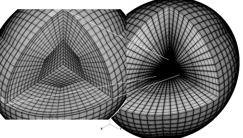
Figure 1: Cut through the global ellipsoidal mesh. In the zoomed part we show the mesh for the fluid domain only, which is more densely packed than for the outer domain.

2 Benchmarks

2.1 Galloway-Proctor Dynamo

In order to validate our implementation of the magnetic vector potential equations, we consider the case of the Galloway-Proctor dynamo (Galloway and Proctor(1992); Cattaneo et al.(1995)Cattaneo, Kim, Proctor, and Tao). We solve the kinematic dynamo problem in a 3D-periodic Cartesian domain of length $(2\pi,2\pi,2\pi/k_{z})$, where $k_{z}=0.57$ is the optimal wave-number for dynamo action. The imposed velocity field is given by

$$u_{x} = -\sin(y+\sin\omega t),$$ (1)

$$u_{y} = -\cos(x+\cos\omega t),$$ (2)

$$u_{z} = \sin(x+\cos\omega t)+\cos(y+\sin\omega t)\ .$$ (3)

This kinematic problem is solved both with our magnetic vector potential approach and with the native MHD solver available with Nek5000 based on Elsasser variables. The domain is made of 128 elements and the order of polynomial used within each element is $N=5$. Our results are also compared with results obtained using classical pseudo-spectral methods (Cattaneo et al.(1995)Cattaneo, Kim, Proctor, and Tao). The initial condition is given by $\mathbf{A}=(0,0,\cos(y)\sin(k_{z}z))$. The growth rates for various magnetic Reynolds numbers are shown in Figure 2. The agreement between the different methods is excellent and validates our implementation of the MHD equations for an idealized periodic case.

S2

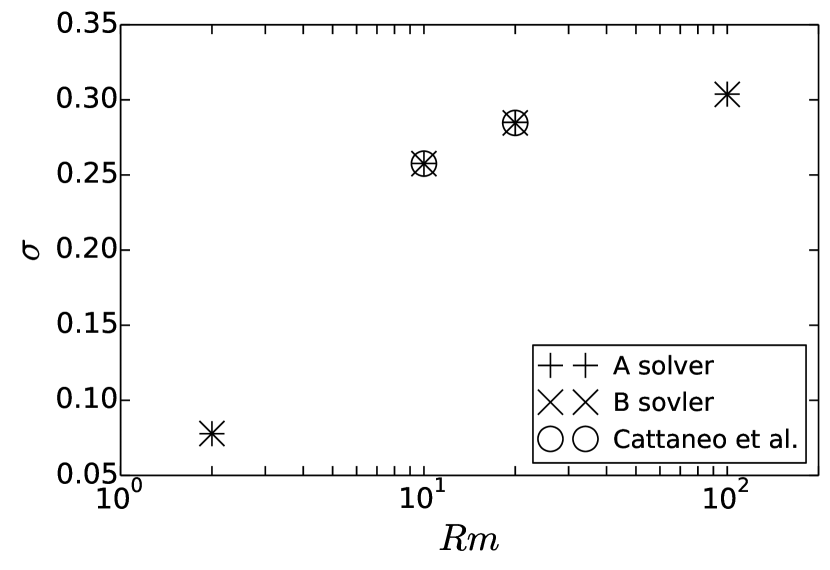
Figure 2: Growth rates of the magnetic field for the Galloway-Proctor kinematic dynamo problem versus the magnetic Reynolds number. $+$ correspond to the vector potential method used in this study. Crosses and hollow circles represent the growth rates obtained from the MHD solver of Nek5000 using Elsasser variables and from Cattaneo et al.(1995)Cattaneo, Kim, Proctor, and Tao, respectively.

2.2 Freely decaying modes in a conducting sphere

In order to check our implementation of the insulating boundary conditions, we consider the purely diffusive decay of a magnetic field inside a conducting sphere of unit radius surrounded by an insulating infinite domain. We thus solve the simple equation $\partial_{t}\mathbf{B}=\nabla^{2}\mathbf{B}$. This linear equation has an infinite set of eigensolutions. The slowest decay occurs for an axial dipole and is given by (see Iskakov et al.(2004)Iskakov, Descombes, and Dormy)

$${\bf B}={\bf B}_{0}\exp(-\pi^{2}t)\ .$$ (4)

Numerically, we solve this problem in a unit sphere surrounded by a larger sphere with radius $\chi=8.5$ and with a magnetic diffusivity increased by a factor $\lambda$. At the outer sphere boundary, we impose $\mathbf{A}=\mathbf{0}$, as in the simulations shown in the paper. The entire domain is made of 1120 elements, including 448 elements for the inner domain, and the order of polynomial used within each element is $N=5$. Our initial condition is an axial dipole of arbitrary amplitude and we consider different diffusivity ratio $\lambda$. Figure 3 shows the relative error between the measured growth rate $\sigma$ from our simulation and the theoretical prediction $\sigma_{\mathrm{th}}$ given by equation (4). As expected, we observe a rapid decrease of the error as $\lambda$ increases, and the relative error is less than $1\%$ when $\lambda=100$, which is the typical value used throughout this paper. This test validates our implementation of the insulating boundary conditions using a multi-domain approach with a jump in the magnetic diffusivity at the boundary of the fluid domain.

S3

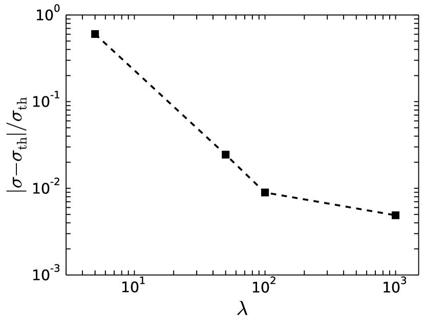
Figure 3: Relative error on the decay rate of an axial dipole in a unit sphere as a function of the diffusivity ratio $\lambda$ between the outer and inner domains.

2.3 Dudley-James dynamos

We now consider a test problem when both advection and diffusion of the magnetic field are involved in a confined domain: the so-called Dudley and James dynamos (Dudley and James(1989)). The induction equation is solved in a unit sphere surrounded by an insulating domain. The imposed flow corresponds to the so-called $s_{2}t_{2}$ case of Dudley and James(1989) (see their equation (24) p.421), which is a simple superposition of selected spherical harmonics with prescribed radial structures. Again, we solve this problem using our numerical approach, fixing $\chi=8.5$, $\lambda=100$ and varying the magnetic diffusivity. The entire domain is made of 1120 elements, including 448 elements for the inner domain, and the order of polynomial used within each element is $N=5$. The initial condition is an equatorial quadrupole of arbitrary amplitude. We compare the growth rate from the eigenproblem solved by Dudley and James(1989) and those obtained with our initial value numerical integration in Figure 4. Despite the moderate numerical resolution used, the agreement is excellent, which further confirms that our values of $\chi$ and $\lambda$ are large enough to efficiently mimic an insulating boundary in a kinematic dynamo configuration.

S4

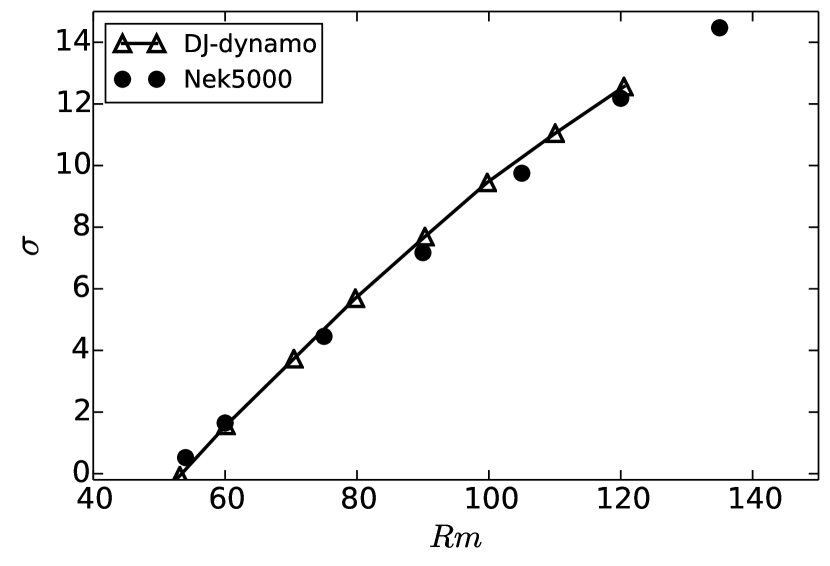
Figure 4: Growth rate of the magnetic field for the kinematic dynamo driven by the $s_{2}t_{2}$ flow. Black triangles represent the growth rates extracted from Fig. 8a of Dudley and James(1989). Black circles correspond to growth rates obtained from our simulations.

3 Numerical convergence

We now discuss how the results shown in this letter depend on our particular choice of numerical and geometric parameters. We focus on the effect of the spatial resolution through the polynomial order $N$. The impact of the aspect ratio $\chi$ and diffusivity ratio $\lambda$ are then considered. In all cases, we consider the particular case $T4$ in Table 1 of the main text, which is a tidally-driven dynamo at $Pm=2$. This case is particularly demanding due to the large magnetic Prandtl number and due to the fact that the outer domain is actually moving (i.e. $\mathbf{u}_{s}\neq\mathbf{0}$ in equation (14)) so that large diffusivity ratio is required to accurately model the outer insulating boundary.

3.1 Convergence with $N$

For case $T4$ in Table 1 of the main text, we performed three simulations which only differ by the polynomial order $N$ to check whether our numerical results are converged. As shown in Figure 5, the resulting growth rate $\sigma$ is nearly the same for $N=7$ and $N=9$. We conclude that the order of polynomial $N=7$ is sufficient to numerically resolve this problem, and use it for the tidally-driven and libration-driven simulations presented in the main paper. For the more requiring precession cases, a similar convergence study led us to use $N=9$.

S5

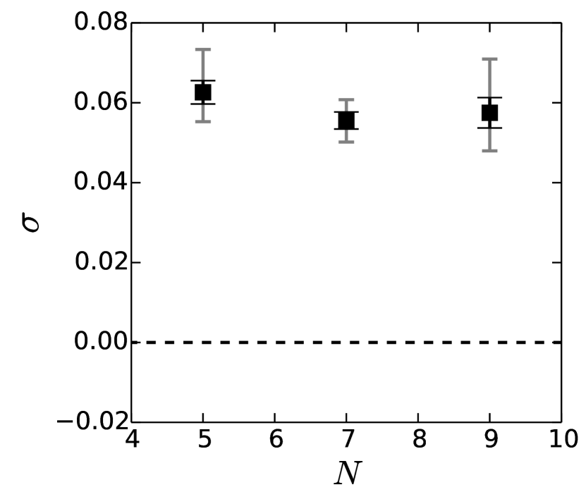
Figure 5: Growth rate $\sigma$ of the magnetic energy as a function of the order of polynomial $N$ within each element of the total domain, for the case T4 in Table 1 of the main text. The black error bars represent one standard deviation and the gray bars represent maximum and minimum estimates.

3.2 Convergence with $\chi$

We now consider the effects of changing the aspect ratio $\chi$ on the solution. We consider different aspect ratios from $\chi=4$ up to $\chi=12$ and compute the growth rate $\sigma$ of the resulting dynamo. The total number of elements in the mesh for $\chi=4$, $8$ and $12$ are $27136$, $28672$ and $30208$, respectively. We keep the number of elements in the fluid the same and fix $N=7$ and $\lambda=100$. In Figure 6, we show the convergence of $\sigma$ with $\chi$. While $\chi=4$ slightly underestimates the growth rate, $\chi=8$ and $\chi=12$ are very similar. We conclude that the choice of $\chi=8$ is sufficient for the artificial effect of the outer boundary to be negligible in our simulations (see also Chan et al.(2007)Chan, Zhang, Li, and Liao).

S6

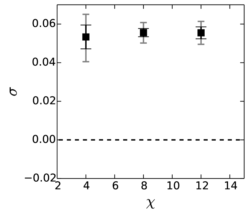
Figure 6: Growth rate $\sigma$ of the magnetic energy as a function of the aspect ratio $\chi$ between the outer and the inner domains, for the case T4 in Table 1 of the main text. The black error bars represent one standard deviation and the gray bars represent maximum and minimum estimates.

3.3 Convergence with $\lambda$

Finally, let us consider the effect of the ratio of diffusivity between the outer and inner domains. The cost of a simulation rapidly goes up with increasing $\lambda$ due to the larger number of iterations required to reach a given convergence threshold. We nevertheless need to choose a large enough ratio $\lambda$ to accurately model the insulating outer domain. In Figure 7, we show the variation of the growth rate $\sigma$, again for case $T4$, for different values of the ratio of diffusivity from $\lambda=50$ up to $\lambda=1000$. Lower values of $\lambda$ are irrelevant and very demanding numerically since the magnetic field topology is more complex and would require an increase in the resolution used in the outer domain. We observe that $\lambda=50$ overestimates the growth rate whereas $\lambda=10^{2}$ is very close to $\lambda=10^{3}$ with a relative error of less that $2\%$. We therefore conclude that using $\lambda=10^{2}$ is enough to accurately model the outer insulating domain.

S7

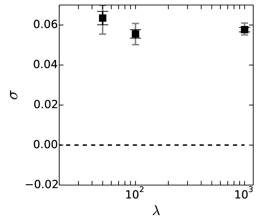
Figure 7: Growth rate $\sigma$ of the magnetic energy as a function of the diffusivity ratio $\lambda$ between the outer and the inner domains, for the case T4 in Table 1 of the main text. The black error bars represent one standard deviation and the gray bars represent maximum and minimum estimates.

References

- [Cattaneo et al.(1995)Cattaneo, Kim, Proctor, and Tao] Cattaneo, F., E.-j. Kim, M. Proctor, and L. Tao (1995), Fluctuations in quasi-two-dimensional fast dynamos, Physical Review Letters, 75(8), 1522.
- [Chan et al.(2007)Chan, Zhang, Li, and Liao] Chan, K. H., K. Zhang, L. Li, and X. Liao (2007), A new generation of convection-driven spherical dynamos using EBE finite element method, Physics of the Earth and Planetary Interiors, 163(1), 251–265.
- [Dudley and James(1989)] Dudley, M. L., and R. W. James (1989), Time-dependent kinematic dynamos with stationary flows, Proceedings of the Royal Society of London A: Mathematical, Physical and Engineering Sciences, 425(1869), 407–429, 10.1098/rspa.1989.0112.
- [Galloway and Proctor(1992)] Galloway, D. J., and M. R. E. Proctor (1992), Numerical calculations of fast dynamos in smooth velocity fields with realistic diffusion, Nature, 356, 691–693.
- [Iskakov et al.(2004)Iskakov, Descombes, and Dormy] Iskakov, A., S. Descombes, and E. Dormy (2004), An integro-differential formulation for magnetic induction in bounded domains: boundary element–finite volume method, Journal of Computational Physics, 197(2), 540–554.