Asymmetric Shapes of Radio Recombination Lines from Ionized Stellar Winds
Abstract
Recombination line profile shapes are derived for ionized spherical stellar winds at radio wavelengths. It is assumed that the wind is optically thick owing to free-free opacity. Emission lines of arbitrary optical depth are obtained assuming that the free-free photosphere forms in the outer, constant expansion portion of the wind. Previous works have derived analytic results for isothermal winds when the line and continuum source functions are equal. Here, semi-analytic results are derived for when the source functions are not equal to reveal that line shapes can be asymmetric about line center. A parameter study is presented and applications discussed.
line: profiles \addkeywordradiative transfer \addkeywordstars: early-type \addkeywordstars: winds, outflows \addkeywordradio lines: stars
0.1 Introduction
Radio astronomy has long proven to be an important window into the study of stellar astrophysics, and stellar outflows have been no exception (e.g., Dulk 1995; Güdel 2002; Kurt et al. 2002). For stellar winds a key driver has been the prospect of measuring wind mass-loss rates, , from the excess infrared (IR) and radio continuum emission relative to the stellar atmosphere (e.g., Panagia & Felli 1975; Wright & Barlow 1975). Numerous studies have focused on determining values based on this approach (e.g., Abbott et al. 1980; Abbot, Bieging, & Churchwell 1981; Abbott et al. 1986; Bieging, Abbott, & Churchwell 1989; Leitherer, Chapman, & Koribalski 1995).
One of the main results from a consideration of free-free excesses formed in the wind is that the spectral energy distribution (SED) at long wavelengths will have a power-law slope with flux . However, this outcome depends on several assumptions: isothermal, spherical symmetry, large optical depth, negligible contribution from the stellar atmosphere, and constant outflow speed. Cassinelli & Hartmann (1977) explored the effects of different power laws for the wind density and temperature distributions to relate the SED power-law slope to these influences. Schmid-Burgk (1982) showed that such SED slopes persist even for axisymmetric stellar envelopes, as long as the same power-law relations are adopted. The main difference is that flux levels are modified, which would have implications for inferring values.
Of greater relevance in recent decades has been the abundance of evidence for clumping in massive star winds. In this regard the literature is voluminous, and there has even been a conference to focus on the topic (Hamann, Feldmeier, & Oskinova 2008). The line-driven winds of massive stars (Castor, Abbot, & Klein 1975; Friend & Abbott 1986; Pauldrach, Puls, & Kudritzski 1986) are known to be subject to an instability (e.g., Lucy & White 1980; Owocki, Castor, & Rybicki 1988). This instability produces shocks in the flow and is a natural culprit for stochastic wind clumping. The clumping is well-known to affect the long wavelength emission because of the density-square dependence of the free-free emissivity. In the presence of clumping, the radio emission is overly bright for a given value of as compared to a smooth (i.e., unclumped) wind with the same mass loss. Neglecting the clumping leads to overestimates of , scaling as the square root of the clumping factor, or inverse to the square root of the volume filling factor of clumps. These factors will be defined precisely in the following section.
Clumping affects any density-square emissivity, including recombination lines. Clumping has been incorporated into several detailed complex numerical codes for modeling massive star atmospheres and their winds, such as CMFGEN (Hillier & Miller 1999) and PoWR (Hamann, Gräfener, & Liermann 2006). An important distinction for clumping is between “macroclumping” and “microclumping”. The former leads to modifications of observables that can depend on the shape of the clump and is sometimes synonymous with a “porosity” treatment. The latter is when clumps are all optically thin, so that the radiative transfer does not depend on details of clump morphology. Consequently, microclumping can be handled in terms of a scale parameter, and in fact does not alter the SED slope relative to a unclumped wind (Nugis, Crowther, & Willis 1998). Ignace (2016a) considered the impact of macroclumping vs microclumping for ionized winds at long wavelength.
This contribution is concerned with modeling a radio recombination line (RRL) profile shape that also includes continuum free-free opacity. The problem has been addressed many times before. Rodríguez (1982) derived the line profile shape for this case, with the interest of supplementing the use of the continuum to obtain with line broadening formed in the same spatial locale to obtain the wind terminal speed . Hillier, Jones, & Hyland (1983) did so as well. Ignace (2009) repeated the derivation, and expanded the consideration for inclusion of line blends. All of these treatments assume that the source function for the line and continuum is the same, as given by the Planck function for an isothermal wind. Using a numerical radiative transfer calculation, Viner, Vallee, & Hughes (1979) showed that an asymmetric line shape can result when the line and continuum source functions are unequal. Here, this result is explored further through analytic derivations. Section 0.2 introduces the model assumptions and presents a derivation for the line shape. Unlike most previous treatments, the derivation also allows for a power-law distribution of microclumping in the wind. Section 0.3 provides for a parameter study for line profile shapes. Section 0.4 discusses relevant applications for various astrophysical sources.
0.2 Radio Recombination Line Modeling
Various authors have addressed the relevance of non-LTE effects for interpreting observed RRLs. A discussion of progress on the topic can be found in Gordon & Sorochenko (2002). Relevant to wind-broadened emission lines, Viner et al. undertook a calculation of departure coefficients for studies of H ii regions. As previously noted, they allowed for spherical outflow and found that line shapes can be asymmetric. Peters, Longmore, & Dullemond (2012) conducted a similar study for H ii regions, and elaborated further on line asymmetry for an outflow. However, neither Viner et al. nor Peters et al. explored the possibility of analytic solutions for the radiative transfer. Here, the approach largely follows Ignace (2009), but relaxing the assumption that the line and continuum source functions are equal. The primary assumptions of the model are as follows:
-
i.
The wind is spherically symmetric in time average.
-
ii.
The wind is optically thick to free-free opacity. The line can be thin or thick.
-
iii.
While the line and continuum source functions may not be equal, they are taken as constant with radius.
-
iv.
Microclumping is included in the treatment, specifically as a power-law distribution111The additional power-law distribution need not be attributed to clumping. It could be attributed to something else that modifies the density. However, it cannot be the velocity law, since that would lead to a different geometry for the isovelocity zones and would invalidate the derivation that follows. The inclusion of the additional power law follows the spirit of the approach in Cassinelli & Hartmann (1977). with radius. Clumping in massive star winds is both predicted and measured to vary with radius (e.g., Runacres & Owocki 2002; Blomme et al. 2002, 2003; Puls et al. 2006).

0.2.1 Wind Parameters
Spherical symmetry requires that the wind has a strictly radial wind velocity and density. Being optically thick to free-free opacity, only the large radius flow at constant expansion will be considered. The wind terminal speed is represented by . The wind also has a time-average mass-loss rate of , and the star has radius .
Microclumping is represented as
| (1) |
where represents spatial averaging. On the right-hand side, the average density is given by the smooth wind relation for spherical symmetry, with
| (2) |
For emissivity , the emission is enhanced above the smooth wind by the clumping factor . It is often common to represent the clumping in the wind with a volume filling factor, . Both approaches are used in the literature (c.f., clumping factor: Hamann & Koesterke 1998 or Ignace, Quigley, & Cassinelli 2003; volume filling factor: Abbott et al. 1981 or Dessart et al. 2000).
For this study the clumping factor is allowed to vary with radius as a power law, with
| (3) |
The case of is for clumping that is constant throughout the flow; implies that clumping declines with radius; is the opposite case. (Note that some care must be taken with use of the power law for clumping, since .)
0.2.2 Line and Continuum Opacities
The free-free opacity, , is given by
| (4) |
where is the number density of ions, with the mean molecular weight per free ion; is the number density of electrons, with the mean molecular weight per free electron; is the mass of hydrogen; and (Cox 2001)
| (5) |
In the preceding equation, is Planck’s constant, is the Boltzmann constant, is the temperature of the gas appropriate for the continuum emission, is the root mean square ion charge, is frequency, and is the Gaunt factor.
Figure 1 shows the geometry for evaluating the optical depth along a ray. Cylindrical coordinates for the observer are , with the observer located at great distance along the -axis. Spherical observer coordinates are , with . The continuum optical depth along a ray of fixed impact parameter, , is
| (6) |
where signifies a normalized parameter, in this case and lengths are relative to , and the optical depth scaling is
| (7) |
At long wavelengths that are the focus of this paper, for the Rayleigh-Jeans limit, and .
The line opacity is somewhat similar to that of the continuum in the sense that there is a dependence on the square of density for recombination. Assuming that the wind speed is highly supersonic, the line optical depth can be approximated from Sobolev theory (Sobolev 1960). The line optical depth becomes
| (8) |
where , for a function of temperature appropriate for the line emission, and .
For the case of constant expansion of the wind at , the line-of-sight velocity shift due to the Doppler effect is . It is convenient to introduce a normalized velocity shift with
| (9) |
Also note that . Then the line optical depth becomes
| (10) |
where the power-law dependence of with radius has been substituted into the expression, along with , and is the optical depth scaling for the line. Casting the line optical depth in terms of and will prove useful for solving the radiative transfer problems in the following sections.
0.2.3 Solution for the Case of
When the line and continuum source functions are the same, let . At wavelength , just outside the maximum velocity shift of the line, the flux of continuum emission is given by
| (11) |
where is the emergent intensity as given by
| (12) |
When the wind is optically thick, such that the excess emission from the wind greatly exceeds the attentuated stellar emisison through the wind, the radiative transfer has a well-known solution when there is no clumping (Panagia & Felli 1975; Wright & Barlow 1975). When constant clumping is present (), the spectral energy distribution is unchanged, and the flux is simply enhanced above that of a smooth wind (Nugis et al. 1998).
Ignace (2009) also showed that an analytic solution can result with a power-law distribution in the clumping. The following integral relation will be found of general use in subsequent steps:
| (13) |
where is the Gamma-function.
For the case at hand, the continuum optical depth is
| (14) | |||||
| (15) | |||||
| (16) |
where the second line above uses a change of variable to , with , and
| (17) |
The flux of continuum emission becomes
| (18) |
In the Rayleigh-Jeans limit, the continuum flux will have a power-law slope of , with scaling as for the Planck function. When , the canonical slope of results. Formally, the analytic solution of Equation (18) requires that .
Within the line, the solution is really not any more complicated. Again, Ignace (2009) showed that
| (19) |
While the argument of the exponential now has two terms, the form of the integral is just like that of the pure continuum. The analytic result is
| (20) |
Note that . When , the result of Rodríguez (1982) is recovered. The foremost outcome for when the line and continuum source functions are equal is that regardless of the value of , the line profile is always symmetric about line center. However, when the two source functions are not equal, the line shape will be asymmetric, as demonstrated in the next section.
0.2.4 Solution for the Case of
In the previous section, a relatively complicated radiative transfer problem for line and continuum was found to have an analytic solution. The simplifications required to obtain that solution were spherical symmetry, time-independent flow, and the limit of constant wind expansion. Variation in the clumping factor could be included if the variation can be treated as a power law. Especially key was that both the free-free and line opacities scaled as the square of density.
The final key assumption was that the line and continuum source functions were equal. However, this assumption can be relaxed to allow for unequal source functions (yet still constant throughout the flow at large radius). In this case the solution for the emergent intensity is more complicated, and becomes
| (21) |
This expression has three terms. A ray at impact parameter intersects the conical isovelocity zone in the form of a ring. Considering just one point on this ring corresponding to for a given velocity shift , we have two path segments and one point to consider for the accumulation of sinks and sources that contribute to the emergent intensity. The first term in the expression is for the continuum emission up to the point of interest, and then its attenuation by the line opacity at the point. The second term is for the continuum emission from the point of interest to the observer. The third term is the contribution by the line emission, as attenuated by the foreground continuum opacity. Thus as before, is the total continuum optical depth along the ray, and we also have as the continuum optical depth from the observer to the point of interest where the line emissivity contributes to the emission.
When , terms involving cancel out. With unequal source functions, the dependence on persists. The emergent intensity now becomes:
| (22) |
For this expression the first term closely mimics the result from the preceding section when . Thus the other two terms in the arrangement of Equation (22) represent modifications when the source functions are unequal.
The flux still has an analytic solution. However, an additional standard integral relation is required, of the form
| (23) |
This relation can be applied to the solution for the flux by allowing , for which . One also has with .
The flux in the continuum, outside the velocities of the line, is the same as in the preceding section. However, within the line, the flux now becomes
| (24) | |||||
where
| (25) |
and
| (26) |
It is frequently the case that line profile data are plotted as continuum normalized. The continuum-normalized emission line profile is given by
| (27) | |||||
where
| (28) |
and
| (29) |
where the negative anticipates that the Gamma function in the numerator is also negative.
Note the following special cases. Of course, where there is no line opacity, the radio SED will be a power law in wavelength with
| (30) |
for . The opposite extreme is when the line opacity is significant, but the continuum is negligible. The emission line profile shape becomes
| (31) |
Note that the line shape is symmetric about line center in the limit of a strong line. Wavelength dependence pertinent to the specific line transition is implied through the factors and .


Equation (27) is the main result of this study. The first term represents a symmetric component to the emission line profile. The subsequent two terms contribute generally to asymmetric influences to the line in the form of . These influences depend on the clumping power-law exponent , on the ratio of the source functions , and on the ratio of optical depths . Note that if , the line is in emission, whereas for , the line is in absorption. Illustrative examples are given in the following section.
0.3 Results
Figures 2–4 provide illustrative results for line profile shapes. Figure 2 is for (i.e., clumping that increases with radius); Figure 3 is for (i.e., clumping that is constant with radius); and Figure 4 is for (i.e., clumping that declines with radius). Each figure has 4 panels: upper left is for , lower left is for , upper right is for , and lower right is for for Figures 2 and 3, but and 1.4 for Figure 4. Each panel has 5 line profiles, with and 10, from the weakest line to the strongest. The profiles are continuum normalized and plotted against velocity shift, . Note that each panel has a different ordinate scale.

In the case that , the line profile is actually in absorption. In the case of , the line shape takes the appearance of a weak P Cygni line shape, with blueshifted net absorption and redshifted net emission.
For , the line profiles are more symmetric about line center as compared to either or . As approaches , the line profile becomes perfectly symmetric, because the factor contributing to the line asymmetry cancels exactly when . As increases, the line shapes become increasingly asymmetric with the line skewed preferentially toward blueshifted velocities. This is natural generally because the attentuation of line emission from the farside hemisphere of the wind is greater than from the nearside hemisphere. When , absorption is exactly compensated by emission, and no asymmetry in the line can result. For the given assumptions, the line asymmetry occurs only when the source functions are unequal.
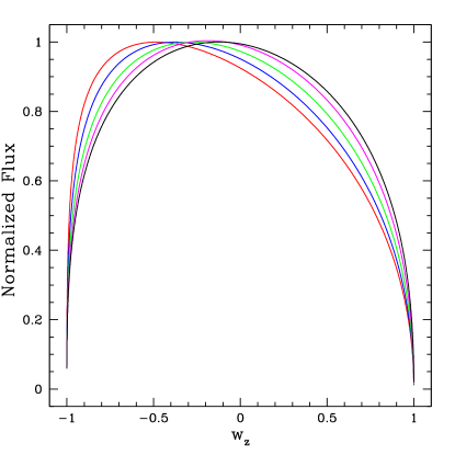
The line profiles display some degeneracy between and . As becomes large, asymmetry in the line shape lessens, in the sense that the peak emission shifts closer to line center. A large line optical depth means that (positive) has less influence on the line shape. Generally, controls the degree of asymmetry in the line, and acts as an overall amplitude for the line emission (or line equivalent width).
0.4 Conclusions
The focus of this contribution has been to highlight the asymmetry of RRLs arising from a spherical wind using an analytic derivation. Previous analytic work produced symmetric line shapes. Numerical calculations have demonstrated that asymmetric lines can be produced. Here, with the assumption of constant but unequal line and continuum source functions, asymmetric line shapes are produced. The derivation allows for the presence of microclumping in the wind in terms of a power-law distribution (rising or declining with radius from the star). While the clumping distribution can impact line asymmetry, the line asymmetry results even with constant clumping, or no clumping whatsoever. Under the model assumptions, emission line asymmetry arises from the continuum opacity (specifically the appearance of the term with in Equation [27]) that absorbs the redshifted emission from the far hemisphere more than the blueshifted emission from the near hemisphere. The result is a line shape with blueshifted emission peak. (The same effect arises in X-ray lines; c.f., Ignace 2016b).
RRLs are vigorously pursued as a diagnostic of source properties, from kinematics to geometrical aspects. Peters, Longmore, & Dullemond (2012) have made an indepth study of various factors that affect the flux of line emission and the shape of the line profile, including line asymmetry. Observational motivation for understanding line asymmetry of RRLs include some objects as the early-type binary MWC349, specifically the H76 line (Escalante et al. 1989). Understanding the line formation is key for distinguishing between radiative transfer effects for the line formation versus the influence of aspherical effects intrinsic to the source, such as binarity or asymmetric mass-loss or flow geometry. Applications for such effects include emission-line objects like MWC349 (e.g., LkH 101; Thum et al. 2013), outflow from star-forming clumps (e.g., Kim et al. 2018), and Planetary Nebulae (e.g., Ershov & Berulis 1989; Sánchez Contreras et al. 2017). Analytic solutions are valuable to these studies in two main respects: (a) they allow for rapid evaluation of parameter space that can be honed with more detailed numerical calculations to fit data, and (b) they are important for providing non-trivial benchmarks against which numerical codes can be tested.
Acknowledgements.
The author expresses appreciation to an anonymous referee for several helpful comments.References
- (1) Abbott D. C., Bieging J. H., Churchwell E., Cassinelli, J. P., 1980, ApJ, 238, 196
- (2) Abbott D. C., Bieging J. H., Churchwell E. B., 1981, ApJ, 250, 645
- (3) Abbott, D., Bieging, J., Churchwell, E., Torres, A., 1986, ApJ, 280, 671
- (4) Bieging, J., Abbott, D., Churchwell, E., 1989, ApJ, 340, 518
- (5) Blomme, R., Prinja, R., Runacres, M., Colley, S., 2002, A&A, 382, 921
- (6) Blomme, R., van de Steene, G., Prinja, R., Runacres, M., Clark, J., 2003, A&A, 408, 715
- (7) Cassinelli, J. P., Hartmann, L., 1977, ApJ, 212, 488
- (8) Castor, J., Abbott, D., Klein, R., 1975, ApJ, 195, 157
- (9) Cox, A. (ed.), 2000, “Allen’s Astrophysical Quantities,” (New York: AIP Press, Spring)
- (10) Dessart, L., Crowther, P., Hillier, D., Willis, A., Morris, P., van der Hucht, K., 2000, MNRAS, 315, 407
- (11) Dulk, G. A., 1985, ARA&A, 23, 169
- (12) Escalante, V., Rodrìguez, L., Moran, J., Canto, J., 1989, RmxAA, 17, 11
- (13) Friend, D., Abbott, D., 1986, ApJ, 311, 701
- (14) Gordon, M., Sorochenko, R., 2002, “Radio Recombination Lines. Their Physics and Astronomical Applications,” (Kluwer: Dordrecht)
- (15) Güdel, M., 2002, ARA&A, 40, 217
- (16) Hamann, W.-R., Koesterke, L., 1998, A&A, 335, 1003
- (17) Hamann, W.-R., Feldmeier, A., Oskinova, L. (eds.), 2008, “Clumping in Hot-Star Winds” (Potsdam: Universitätsverlag Potsdam)
- (18) Hamann, W.-R., Gräfener, G., Liermann, A., 2006, A&A, 457, 1015
- (19) Hillier D. I., Jones, T. J., Hyland, A. R., 1983, ApJ, 271, 221
- (20) Hillier, D. I., Miller, D. L., 1999, ApJ, 519, 354
- (21) Ignace, R., 2009, Astronomische Nachrichten, 330, 717
- (22) Ignace, R., 2016a, MNRAS, 457, 4123
- (23) Ignace, R., 2016b, AdSpR, 58, 694
- (24) Kim, W.-J., Urquhart, J., Wyrowski, F., Menten, K., Csengeri, T., 2018, A&A, 616, A107
- (25) Leitherer, C., Chapman, J. M., Koribalski, B., 1995, ApJ, 450, 289
- (26) Lucy, L., White, r., 1980, ApJ, 241, 300
- (27) Nugis T., Crowther P. A., Willis A. J., 1998, A&A, 333, 956
- (28) Owocki, S., Castor, J., Rybicki, G., 1988, ApJ, 335, 914
- (29) Panagia, N., Felli, M., 1975, A&A, 39, 1
- (30) Pauldrach, A., Puls, J., Kudritzki, R., 1986, A&A, 164, 86
- (31) Puls, J., Markova, N., Scuderi, S., Stanghellini, C., Taranova, O., Burnley, A., Howarth, I., 2006, A&A, 454, 625
- (32) Rodríguez, L., 1982, RMxAA, 5, 179
- (33) Runacres, M., Owocki, S., 2002, A&A, 381, 1015
- (34) Sánchez Contreras, C., Báez-Rubio, A., Alcolea, J., Bujarrabal, V., martín-Pintado, J., 2017, A&A, 603, A67
- (35) Sobolev, V., 1960, “Moving Envelopes of Stars” (Cambridge: Harvard University Press)
- (36) Peters, P., Longmore, S., Dullemond, C., 2012, MNRAS, 425, 2352
- (37) Thum, C, Neri, R., Báez-Rubio, A., Krips, M., 2013, A&A, 556, A129
- (38) Weiler, K., Panagia, N., Monte, M., Sramek, R., 2002, ARA&A, 40, 387
- (39) Wright, A. E., Barlow, M. J., 1975, MNRAS, 170, 41