A Unified Perspective of Evolutionary Game Dynamics Using Generalized Growth Transforms

Abstract

In this paper, we show that different types of evolutionary game dynamics are, in principle, special cases of a dynamical system model based on our previously reported framework of generalized growth transforms. The framework shows that different dynamics arise as a result of minimizing a population energy such that the population as a whole evolves to reach the most stable state. By introducing a population dependent time-constant in the generalized growth transform model, the proposed framework can be used to explain a vast repertoire of evolutionary dynamics, including some novel forms of game dynamics with non-linear payoffs.

I Introduction

Evolutionary games utilize classical game theoretic concepts to describe how a given population evolves over time as a result of interactions between the members of the population. The fitness of an individual in the population is governed by the nature of these interactions, and in accordance with the Darwinian tenets of evolution[1, 2]. For instance, in a strategic game each individual receives a payoff or gain according to the survival strategy it employs, as a result of which the traits or strategies with the maximum payoffs eventually dominate the population through reproduction, mutation, selection or cultural imitation. These principles of evolutionary game dynamics have been applied to different applications ranging from genetics, social networks, neuroeconomics to congestion control and wireless communications [2, 3, 4, 5, 6, 7, 8, 9, 10, 11, 12, 13].

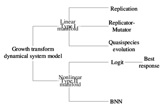
Figure 1: Illustration of the scope of the paper: Most of the commonly known evolutionary stable game dynamics can be obtained from the generalized growth transform dynamical system model, by using different forms of cost functions, adaptive time constants and manifolds.

In literature, numerous mathematical models have been proposed to describe the evolutionary process [14, 15, 16, 2, 17] and are briefly summarized in Figure 1. Each of these models subsumes different set of assumptions on the types of strategies and payoffs that the population employs in the course of evolution. However, all of these formulations can be mathematically expressed as a dynamical system model which for stable games eventually converges to a stationary point on the probability simplex defined by the available strategies in the population. The dynamics are inherently nonlinear in the most generic case, and the existence of Nash equilibria(NE) or of Evolutionarily Stable States(ESSs) depends on the nature of the inter-species interactions[18, 19, 2]. In this paper, we report that many of these evolutionary game models are special cases of our previously reported framework of a growth transform based dynamical system model [20], as illustrated in Figure 1. The framework was derived from an energy minimization-based perspective that exploited the inherent tendency of all natural systems to evolve to their most stable state (which is also the state where the system has the minimum free energy) subject to different conservation constraints [21, 22]. In this paper, we can extend the same argument to a population/network where individuals interact with each other to reach the population level most stable configuration in an energy landscape. The approach is thus similar in flavor to the concept of congestion games, and more generally potential games, which map the Nash equilibria of a game to the locally optimal points of a corresponding Lyapunov or potential function. For stable potential games involving strictly concave potentials, a unique Nash equilibrium always exists [23, 24, 25, 16]. Section II gives an overview of the generalized growth transform dynamical system model. In this paper, we demonstrate how most of the commonly studied evolutionary dynamics are special cases of the growth transform based dynamical system model. Growth transforms have been applied previously for solving replicator equations with linear payoffs and in discrete-time scenarios [26, 27, 28, 14]. In Section III we demonstrate how different types of known evolutionary dynamics like replicator dynamics with nonlinear payoffs, imitation games, best response dynamics, Brown-von-Neumann dynamics etc. can all be derived from the generic growth transform dynamical system model, in addition to generation of several interesting types of hitherto unexplored ones.

II Main Result

In [20], we used the Baum-Eagon inequality[29] to show that an optimal point of a generic Lipschitz continuous cost function $H(\mathbf{p}),\mathbf{p}\in D\subset\mathbb{R}^{N}$, where $D=\{\mathbf{p}\in\mathbb{R_{+}}^{N}:p_{i}\geq 0,\quad\sum\limits_{i=1}^{N}p_{i}=1\}$, corresponds to the steady state solution of the generalized growth transform dynamical system model with time-constant $\tau>0$, given by

$$\tau\dot{p}_{i}+p_{i}=\dfrac{p_{i}\Bigg{[}-\dfrac{\partial H(\mathbf{p})}{\partial p_{i}}+\lambda\Bigg{]}}{\sum\limits_{i}p_{i}\Bigg{[}-\dfrac{\partial H(\mathbf{p})}{\partial p_{i}}+\lambda\Bigg{]}},$$ (1)

The above equation can be rewritten in a compact form as follows

$$\tau\dot{p}_{i}=p_{i}\Bigg{[}\dfrac{f_{i}(\mathbf{p})}{\bar{f}}-1\Bigg{]},$$ (2)

where $f_{i}(\mathbf{p})=\Bigg{[}-\dfrac{\partial H(\mathbf{p})}{\partial p_{i}}+\lambda\Bigg{]}\quad\forall i$ and $\bar{f}=\sum_{i}p_{i}f_{i}(\mathbf{p})$. The constant $\lambda\in\mathbb{R}_{+}$ is chosen to ensure that $f_{i}(\mathbf{p})>0,\forall i$.

However, the convergence of Equation (1) to the steady-state solution also holds if the time-constant $\tau$ is also varied with time. This is because the normalization constraint is the only condition on the population state at any instant of time so as to ensure that the manifold $D$ is an invariant manifold, and hence other types of time constants can also be used, provided it is identical for all the strategies. If different strategies evolve according to different time constants, however, convergence to a locally optimal solution for Lipschitz continuous cost functions is not guaranteed. In this paper we will vary $\tau$ as a function of $\mathbf{p}$ such that $\tau=\dfrac{1}{\bar{g}(\mathbf{p})}$, where $\bar{g}(\mathbf{p})>0$ could be an arbitrary time-varying function. Substituting for $\tau$ in Equation (2) we arrive at the key dynamical system model equation:

$$\dot{p}_{i}=p_{i}\Bigg{[}\dfrac{f_{i}(\mathbf{p})}{\bar{f}}\bar{g}(\mathbf{p})-\bar{g}(\mathbf{p})\Bigg{]}.$$ (3)

We will now show that Equation (3) can be used to explain different evolutionary game dynamics reported in literature and also for proposing some new forms of dynamics.

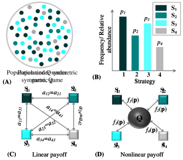
Figure 2: Illustration of a symmetric game setup with four pure strategies: (a)Population at any instant of time (colors denote the strategy each individual adopts at any time $t$); (b)Histogram showing the relative abundance of the strategies in the population, $p_{1}-p_{4}$; (c)Linear payoff case, where the payoff of an individual with strategy $i$ playing against another with startegy $j$ is given by $a_{ij}$, with the fitness of $i$ being $\sum\limits_{j}a_{ij}p_{j}$; (d)Nonlinear payoff case, where each strategy $i$ has a fitness $f_{i}(\mathbf{p})$ against the population $Q$.

III Evolutionary Game Dynamics

We first introduce some mathematical notations and terminology pertaining to evolutionary dynamics arising in the context of deterministic games [2, 3, 14]. In deterministic games, the Nash equilibrium (if it exists), remains unchanged even when perturbed by a small percentage of mutants or external agents playing a different strategy. Also, we will only consider stable games that converge to a global and stable Nash equilibrium[16, 25].

Consider an infinitely large population with a finite set $\mathbf{S}=\{1,\ldots,N\}$ of $N$ pure strategies available to each individual of the population. The $i^{th}$ strategy is then quantified using a relative abundance measure $p_{i}\in\mathbb{R}_{+}$ and a fitness function (or expected payoff) $f_{i}(\mathbf{p})$ ($f_{i}:\mathbb{R}_{+}^{N}\mapsto\mathbb{R}_{+}$), where $\mathbf{p}\in D$ is the set with elements $p_{i}$. It should be noted here that though the fitness is a function of the relative abundances of various strategies adopted by the population in the most generic case, constant fitness scenarios are also possible in certain types of evolutionary games. Also, for most of the dynamics discussed in this paper, we will consider symmetric games, where all individuals have the same strategy set $\mathbf{S}$ during the course of evolution. Figure 2(a) shows an example of a symmetric game comprising of four pure strategies, where each color denotes the strategy that each individual in the population $Q$ adopts at any instant of time. Figure 2(b) shows the relative abundance $p_{i}$ for each strategy in the population and Figure 2(c) shows an example of a linear payoff function. In this case, each individual which plays a strategy $i$ against any random member of the population playing a strategy $j$ receives a constant payoff $a_{ij}$. The average payoff or fitness of the $i-$th strategy is then given by $\sum\limits_{j}a_{ij}p_{j}$ . Figure 2(d) illustrates a more general payoff scenario, where the average payoff corresponding to the $i-th$ strategy could be a non-linear function $f_{i}(\mathbf{p})$.

Next, we present some of the most common types of evolutionary game dynamics existing in literature, and their relation to the growth transform dynamical system model proposed in Equation (3) by choosing the function $\bar{g}(\mathbf{p})$ to be directly proportional to the instantaneous mean payoff of the population, and using different forms of the cost function $H$.

III-A Replicator dynamics

Replicator dynamics [30] model the case where evolution occurs by pure natural selection, and the fitness of the individual is governed by the frequencies of other strategies in the population. The population thus evolves in a way as to promote strategies having payoffs higher than the mean payoff at any instance of time. The generic form of replicator dynamics with a nonlinear fitness function is given by:

$$\dot{p}_{i}=p_{i}[f_{i}(\mathbf{p})-\bar{f}],\quad\bar{f}=\sum\limits_{i}p_{i}f_{i}(\mathbf{p})$$ (4)

The replicator dynamics can be derived from the growth transform dynamical system model by considering $\bar{g}(\mathbf{p})=\sum\limits_{i}p_{i}(f_{i}(\mathbf{p})+\lambda)$ and a network level cost function of the form

$$H(\mathbf{p})=-\sum\limits_{i}\int_{c}^{p_{i}}f_{i}(\mathbf{z})dz_{i}-\lambda\sum\limits_{i}p_{i},$$ (5)

where $f_{i}(\mathbf{p})$ is a smooth monotonic function of $p_{i}$, and $\lambda>0$ is chosen so as to ensure $f_{i}(\mathbf{p})>0$, and can be thought of as a constant background payoff. Note that $f_{i}(\mathbf{z})=f_{i}(p_{1},\ldots,z_{i},\ldots,p_{n})\quad\forall i$, where $z_{i}$ is a dummy variable corresponding to the $i-$th strategy.

Of particular interest are the replicator dynamics under a linear payoff scenario with a constant payoff matrix $\mathbf{A}$ in a symmetric game ($a_{ij}$ being the fitness of strategy $i$ against any other strategy $j$) and $(\mathbf{Ap}_{i})$ being the fitness or average payoff of strategy $S_{i}$. This can be derived from the growth transform dynamical system model by using $\bar{g}(\mathbf{p})=\sum_{i}p_{i}((\mathbf{Ap})_{i}+\lambda)$ and a cost function of the form $H(\mathbf{p})=-\mathbf{p}^{T}\mathbf{Ap}-\lambda\sum\limits_{i}p_{i}$ over the probabilistic domain $D$. The corresponding dynamics are given by:

$$\dot{p}_{i}=p_{i}[(\mathbf{Ap})_{i}-\mathbf{p}^{T}\mathbf{Ap}]$$ (6)

In [26, 31], the discrete-time version of Equation (6) given by

$$p_{i}(t+1)=p_{i}(t)\dfrac{\mathbf{Ap}(t)_{i}+\lambda}{\sum\limits_{i}p_{i}(t)(\mathbf{Ap}(t)_{i}+\lambda)},$$ (7)

where $\lambda$ is a constant baseline payoff, was shown to be a special case of the Baum-Eagon inequality, and was employed for solving maximum clique and graph isomorphism problems which are commonly encountered in computer vision [28, 26, 27, 32].

The Lotka-Volterra equation can also be derived from the linear payoff form of the replicator equation by means of a simple linear transformation.

III-B Quasispecies evolution

These dynamics correspond to a constant fitness landscape [33], where replications from one generation to the next are error-prone with a high enough mutation rate, i.e., the $j-$th strategy can mutate to the $i-$th strategy with a probability $m_{ji}$. Forward and backward mutations are equally probable in this model, i.e., the mutation matrix $\mathbf{M}=\{m_{ij}\}$ is a doubly stochastic symmetric matrix, with $m_{ij}=m_{ji}$, and $\sum\limits_{i}m_{ij}=\sum\limits_{j}m_{ij}=1$. The dynamical system corresponding to this model of evolution is as follows :

$$\dot{p}_{i}=\sum\limits_{j}p_{j}f_{j}m_{ji}-p_{i}\sum\limits_{i}p_{i}f_{i},\quad\sum\limits_{i}m_{ji}=1\enskip\forall i$$ (8)

Noting that the mutation matrix $\mathbf{M}$ is doubly stochastic and that each strategy has a constant fitness, the quasispecies dynamics can be achieved by using $\bar{g}(\mathbf{p})=\sum\limits_{i}p_{i}[f_{i}+\lambda]$ and a cost function of the form

$$H(\mathbf{p})=-\sum\limits_{i}\log(p_{i})\sum\limits_{j}p_{j}f_{j}m_{ji}-\lambda\sum\limits_{i}p_{i},$$ (9)

since $\sum\limits_{i}m_{ji}=1$.

III-C Replicator-mutator dynamics

When both replication and mutation contribute to the evolutionary process, we arrive at the replicator-mutator equation [34]:

$$\dot{p}_{i}=\sum\limits_{j}p_{j}f_{j}(\mathbf{p})m_{ji}-p_{i}\sum\limits_{i}p_{i}f_{i}(\mathbf{p}),\quad\sum\limits_{i}m_{ji}=1\enskip\forall i$$ (10)

In a fashion similar to the previous two types of evolutionary dynamics, the mathematical equation governing the replicator-mutator model can be arrived at by considering and time constant $\bar{g}(\mathbf{p})=\sum\limits_{i}p_{i}[f_{i}(\mathbf{p})+\lambda]$ and a cost function of the form

$$H(\mathbf{p})=-\sum\limits_{i}\int_{c}^{p_{i}}\sum\limits_{j}p_{j}f_{j}(\mathbf{z})m_{ij}dz_{i}-\lambda\sum\limits_{i}p_{i}.$$ (11)

The above three examples belong to a more general class of evolutionary dynamics called imitation games, which are of the form $\dot{p}_{i}=p_{i}\zeta_{i}(\mathbf{p})$, with $\sum_{i}p_{i}\zeta_{i}(\mathbf{p})=0\quad\forall\mathbf{p}\in D$.

III-D Logit dynamics and best response dynamics

The logit dynamics [35] represent a class of evolutionary games where the individuals have a partial knowledge about the global state of the system, with a parameter $\eta>0$ representing the noise level of the system. At each step, an individual selects a strategy so as to select the current best response, depending on the noisy population-level knowledge that it possesses. The dynamics of this form are given by:

$$\dot{p}_{i}=\dfrac{\exp(f_{i}(\mathbf{p})/{\eta})}{\sum\limits_{i}\exp(f_{i}(\mathbf{p})/{\eta})}-p_{i}$$ (12)

For noiseless systems, i.e., when $\eta\to 0$, this converges to the best response dynamics [36], where each individual chooses the best available strategy with the highest probability. A discrete time version of the best response dynamics is the fictitious play [37].

For arriving at the Logit dynamics from the growth transform model, we choose $\bar{g}(\mathbf{p})=\sum\limits_{i}\exp(f_{i}(\mathbf{p})/\eta)$ a cost function of the form:

$$H(\mathbf{p})=-\sum\limits_{i}\int_{c}^{p_{i}}\dfrac{1}{z_{i}}\exp{f_{i}(\mathbf{z}/\eta)}dz_{i},\quad p_{i}>0\enskip\forall i,$$ (13)

where $f_{i}(\mathbf{z})$ has the same definition as in the replicator dynamics case.

III-E Brown-von Neumann-Nash (BNN) dynamics

When each strategy gets updated only if its payoff is greater that the average payoff of the population with a certain margin $\epsilon$, we obtain the following equation which corresponds to the Brown-von Neumann-Nash dynamics [38]:

$$\dot{p}_{i}=k_{i}(\mathbf{p})-p_{i}\sum\limits_{i}k_{i}(\mathbf{p})$$ (14)

where $k_{i}(\mathbf{p})=\max(0,((\mathbf{Ap})_{i}-\mathbf{p}^{T}\mathbf{Ap}+\epsilon))$.

The BNN dynamics, similarly, can be achieved by considering $\bar{g}(\mathbf{p})=\sum\limits_{i}k_{i}(\exp(\mathbf{x}))$ and a cost function of the form:

$$H(\mathbf{p})=-\sum\limits_{i}\int_{c}^{p_{i}}\dfrac{1}{z_{i}}k_{i}(\mathbf{z})dz_{i}$$ (15)

where $k_{i}(\mathbf{p})=\max(0,((\mathbf{Ap})_{i}-\mathbf{p}^{T}\mathbf{Ap}+\epsilon))$ as before, and $p_{i}>0\enskip\forall i$.

III-F Unconventional and novel dynamics

Novel types of evolutionary dynamics can be arrived at by using other forms of the function $\bar{g}(\mathbf{p})$, and also by using other variants of the cost function. A particularly interesting scenario uses a cost function $H(\mathbf{p})=-\sum\limits_{i}\int_{c}^{p_{i}}h(z_{i})f_{i}(\mathbf{z})dz_{i}$, which leads to a dynamical system of the form:

$$\dot{p}_{i}=p_{i}\Bigg{[}\dfrac{f_{i}^{\prime}(\mathbf{p})}{\bar{f^{\prime}}}\bar{g}(\mathbf{p})-\bar{g}(\mathbf{p})\Bigg{]},$$ (16)

where $f_{i}^{\prime}(\mathbf{p})=h(p_{i})f_{i}(\mathbf{p})=h(p_{i})\Bigg{[}-\dfrac{\partial H}{\partial p_{i}}+\lambda\Bigg{]}\quad\forall i$.

We can choose a form of $h(p_{i})\quad\forall i$ such that only a certain sub-population is selected to determine the mean fitness of the entire population. Potential candidates for the form of the functions $h(\cdot)$ include derivatives of smooth saturation functions like the hyperbolic tangent function, the logistic function, the sigmoidal function, the softmax function etc. For example, using $h(p_{i})=\sech^{2}(p_{i})$ (which corresponds to the derivative of the hyperbolic tangent function) in Equation (3) would lead to $f_{i}^{\prime}(\mathbf{p})=\sech^{2}(p_{i})f_{i}(\mathbf{p})$, which updates only certain members of the population instead of the entire population, as in the case of the standard evolutionary games. Though such types of optimization problems do not necessarily have a globally optimal solution due to the non-convexity of the domain and/or the objective function under consideration, convergence to a locally optimal solution is always guaranteed in such cases. Intuitively, this implies that even when each strategy in the population gets updated with limited information about the overall population behavior, the population will converge to a locally stable solution eventually. The concept is thus similar in essence to the lattice based population dynamics [39, 40] approach, where each individual updates its strategy based only on the strategies of a certain number of players in its local neighborhood, which can be described by a graph or by a lattice structure. Such neighborhood based models which allow local interactions and dispersal and operate at relatively smaller spatial scales were shown to promote coexistence of strategies leading to biodiversity [41], since dominated strategies in such scenarios can form isolated clusters or can survive by moving over time to a spatially different location in the lattice structure [2].

IV Discussions and Conclusions

In this paper, we used an energy minimization framework based on the generalized growth transform dynamical system model to explain different types of network dynamics for stable evolutionary games having a unique strictly stable Nash equilibrium. We also showed how unexplored evolutionary processes can also be mapped to a growth transform dynamical system with an adaptive time constant, using different variants of the underlying cost function and domain of definition. In this regard the optimal point of the objective function can be related to the Nash equilibrium and the evoluationaly stable state (ESS) of the evolutionary game.

A Nash equilibrium of a game corresponds to the set of strategies adopted by a population such that any deviation from it in the subsequent stages would not result in an increased payoff against the current strategy. An ESS, on the other hand, is a population state which is inherently stable in the sense that it cannot be invaded by a small group of mutants playing the same strategy. While an ESS is always a Nash equilibrium, the converse is not necessarily true, and only holds for strict Nash equilibria [2, 18]. In the context of the growth transform based formulation, we can conclude the following correspondence between the cost function $H$ and the nature of the equilibria:

• A generic Lipschitz continuous cost function over a convex domain might have multiple local minima, which correspond to the Nash equilibria of the game, and do not necessarily imply evolutionary stability.

• A general convex cost function over a convex domain has a set of Nash equilibria which are always stable for the types of dynamics discussed in the paper, and globally stable for BR and BNN dynamics in particular.

• A strictly convex objective function over a convex domain has a unique strict Nash equilibrium which is also the ESS, and is globally stable for all types of evolutionary dynamics discussed in this paper.

• A strictly concave cost function over a convex domain leads to a locally or globally repelling Nash equilibrium.

Future directions will involve extension of the proposed dynamical system framework for incorporate continuous strategy spaces leading to adaptive dynamics, and scenarios involving multiple types of equilibria.

References

- [1] M. A. Nowak and K. Sigmund, “Evolutionary dynamics of biological games,” Science, vol. 303, no. 5659, pp. 793–799, 2004.
- [2] J. Hofbauer and K. Sigmund, “Evolutionary game dynamics,” Bulletin of the American Mathematical Society, vol. 40, no. 4, pp. 479–519, 2003.
- [3] K. M. Page and M. A. Nowak, “Unifying evolutionary dynamics,” Journal of theoretical biology, vol. 219, no. 1, pp. 93–98, 2002.
- [4] D. Basanta, M. Simon, H. Hatzikirou, and A. Deutsch, “Evolutionary game theory elucidates the role of glycolysis in glioma progression and invasion,” Cell proliferation, vol. 41, no. 6, pp. 980–987, 2008.
- [5] E. Frey, “Evolutionary game theory: Theoretical concepts and applications to microbial communities,” Physica A: Statistical Mechanics and its Applications, vol. 389, no. 20, pp. 4265–4298, 2010.
- [6] A. R. Zomorrodi and D. Segrè, “Genome-driven evolutionary game theory helps understand the rise of metabolic interdependencies in microbial communities,” Nature Communications, vol. 8, no. 1, p. 1563, 2017.
- [7] Z. Han, D. Niyato, W. Saad, T. Başar, and A. Hjørungnes, Game theory in wireless and communication networks: theory, models, and applications. Cambridge university press, 2012.
- [8] D. Friedman, “On economic applications of evolutionary game theory,” Journal of Evolutionary Economics, vol. 8, no. 1, pp. 15–43, 1998.
- [9] A. Byde, “Applying evolutionary game theory to auction mechanism design,” in E-Commerce, 2003. CEC 2003. IEEE International Conference on, pp. 347–354, IEEE, 2003.
- [10] G. Luazuaroiu, A. Pera, R. O. Ștefuanescu Mihuailua, N. Mircicua, and O. Neguritua, “Can neuroscience assist us in constructing better patterns of economic decision-making?,” Frontiers in behavioral neuroscience, vol. 11, p. 188, 2017.
- [11] P. W. Glimcher and A. Rustichini, “Neuroeconomics: the consilience of brain and decision,” Science, vol. 306, no. 5695, pp. 447–452, 2004.
- [12] C. F. Camerer, “Strategizing in the brain,” Science, vol. 300, no. 5626, pp. 1673–1675, 2003.
- [13] L. P. Sugrue, G. S. Corrado, and W. T. Newsome, “Choosing the greater of two goods: neural currencies for valuation and decision making,” Nature Reviews Neuroscience, vol. 6, no. 5, p. 363, 2005.
- [14] N. Nisan, T. Roughgarden, E. Tardos, and V. V. Vazirani, Algorithmic game theory. Cambridge university press, 2007.
- [15] Y. Cohen and J. Cohen, “Evolutionary game theory and the evolution of neuron populations, ring rates, and decisionmaking,” 2009.
- [16] W. H. Sandholm, “Evolutionary game theory,” in Encyclopedia of Complexity and Systems Science, pp. 3176–3205, Springer, 2009.
- [17] B. Allen, G. Lippner, Y.-T. Chen, B. Fotouhi, N. Momeni, S.-T. Yau, and M. A. Nowak, “Evolutionary dynamics on any population structure,” Nature, vol. 544, no. 7649, p. 227, 2017.
- [18] J. Li, G. Kendall, and R. John, “Computing nash equilibria and evolutionarily stable states of evolutionary games,” IEEE Transactions on Evolutionary Computation, vol. 20, no. 3, pp. 460–469, 2016.
- [19] S. Mihai-Alexandru, G. Noémi, and L. R. Ioana, “Approximation of nash equilibria and the network community structure detection problem,” PloS one, vol. 12, no. 5, p. e0174963, 2017.
- [20] O. Chatterjee and S. Chakrabartty, “Decentralized global optimization based on a growth transform dynamical system model,” IEEE Transactions on Neural Networks and Learning Systems, 2018.
- [21] R. Feynman, The character of physical law. MIT press, 2017.
- [22] K. Friston, “The free-energy principle: a unified brain theory?,” Nature Reviews Neuroscience, vol. 11, no. 2, p. 127, 2010.
- [23] D. Monderer and L. S. Shapley, “Potential games,” Games and economic behavior, vol. 14, no. 1, pp. 124–143, 1996.
- [24] I. Milchtaich, “Congestion games with player-specific payoff functions,” Games and economic behavior, vol. 13, no. 1, pp. 111–124, 1996.
- [25] J. Hofbauer and W. H. Sandholm, “Stable games and their dynamics,” Journal of Economic Theory, vol. 144, no. 4, pp. 1665–1693, 2009.
- [26] M. Pelillo, “Replicator equations, maximal cliques, and graph isomorphism,” in Advances in Neural Information Processing Systems, pp. 550–556, 1999.
- [27] I. M. Bomze and B. M. Pötscher, Game theoretical foundations of evolutionary stability, vol. 324. Springer Science & Business Media, 2013.
- [28] I. M. Bomze, M. Budinich, P. M. Pardalos, and M. Pelillo, “The maximum clique problem,” in Handbook of combinatorial optimization, pp. 1–74, Springer, 1999.
- [29] L. E. Baum and G. Sell, “Growth transformations for functions on manifolds,” Pacific Journal of Mathematics, vol. 27, no. 2, pp. 211–227, 1968.
- [30] P. Schuster and K. Sigmund, “Replicator dynamics,” Journal of theoretical biology, vol. 100, no. 3, pp. 533–538, 1983.
- [31] I. Bomze, M. Pelillo, and V. Stix, “Approximating the maximum weight clique using replicator dynamics,” IEEE Transactions on neural networks, vol. 11, no. 6, pp. 1228–1241, 2000.
- [32] R. Mehta, I. Panageas, G. Piliouras, P. Tetali, and V. V. Vazirani, “Mutation, sexual reproduction and survival in dynamic environments,” in LIPIcs-Leibniz International Proceedings in Informatics, vol. 67, Schloss Dagstuhl-Leibniz-Zentrum fuer Informatik, 2017.
- [33] M. Eigen, J. McCaskill, and P. Schuster, “The molecular quasi-species,” Advances in chemical physics, vol. 75, pp. 149–263, 1989.
- [34] K. Hadeler, “Stable polymorphisms in a selection model with mutation,” SIAM Journal on Applied Mathematics, vol. 41, no. 1, pp. 1–7, 1981.
- [35] C. Alós-Ferrer and N. Netzer, “The logit-response dynamics,” Games and Economic Behavior, vol. 68, no. 2, pp. 413–427, 2010.
- [36] A. Matsui, “Best response dynamics and socially stable strategies,” Journal of Economic Theory, vol. 57, no. 2, pp. 343–362, 1992.
- [37] D. Monderer and L. S. Shapley, “Fictitious play property for games with identical interests,” Journal of economic theory, vol. 68, no. 1, pp. 258–265, 1996.
- [38] J. Hofbauer, J. Oechssler, and F. Riedel, “Brown–von neumann–nash dynamics: the continuous strategy case,” Games and Economic Behavior, vol. 65, no. 2, pp. 406–429, 2009.
- [39] E. Lieberman, C. Hauert, and M. A. Nowak, “Evolutionary dynamics on graphs,” Nature, vol. 433, no. 7023, p. 312, 2005.
- [40] M. A. Nowak, C. E. Tarnita, and T. Antal, “Evolutionary dynamics in structured populations,” Philosophical Transactions of the Royal Society of London B: Biological Sciences, vol. 365, no. 1537, pp. 19–30, 2010.
- [41] B. Kerr, M. A. Riley, M. W. Feldman, and B. J. Bohannan, “Local dispersal promotes biodiversity in a real-life game of rock–paper–scissors,” Nature, vol. 418, no. 6894, p. 171, 2002.