New Inflation in the Landscape and
Typicality of the Observed Cosmic Perturbation

Chien-I Chiang^★♢ and Keisuke Harigaya^★♢♣

^★Berkeley Center for Theoretical Physics, Department of Physics, University of California, Berkeley, CA 94720, USA

^♢Theoretical Physics Group, Lawrence Berkeley National Laboratory, Berkeley, California, USA

^♣School of Natural Sciences, Institute for Advanced Study, Princeton, NJ 08540, USA

  Abstract
We investigate if the observed small and nearly scale-invariant primordial cosmic perturbation, i.e.  the perturbation amplitude $P_{\zeta}\sim 10^{-9}$ and the spectral index $n_{s}\simeq 0.965$, is typical in the landscape of vacua after imposing anthropic selections on them. We consider the situation where the universe begins from a metastable vacuum driving a precedent inflation, a curvature-dominated open universe is created by tunneling, and the curvature energy is inflated away by new inflation. We argue that the initial inflaton field value is homogeneous but typically non-zero because of the quantum fluctuation of long wavelength modes created during the precedent inflation, and only the universe which accidentally has a small inflaton field value is anthropically selected. We show that this bias, together with certain distributions of inflation model parameters that are physically well-motivated, makes the observed small and nearly scale-invariant spectrum typical.

 

 

 

1 Introduction

Inflationary paradigm not only solves the horizon and flatness problem [1] (see also [2]), but also elegantly explains the nearly scale-invariant and Gaussian cosmic perturbation imprinted in the cosmic microwave background (CMB) and the large scale structure of the universe [3, 4, 5, 6, 7], given that inflation is driven by a scalar field with a very flat potential [8, 9] (see also [10]). However, despite the phenomenological success of the generic paradigm, the underlying physical origin of cosmic inflation is still an open problem.

We investigate the inflation paradigm in the view point of the string landscape (see [11] for a review). The string theory predicts that there are numerous vacua, and each vacuum yields an effective field theory with a different set of fields and parameters. An example leading to various cosmological constants is given in [12]. The landscape of vacua supports the notion of the anthropic principle. The parameters of the nature which we observe is not necessarily explained by the dynamics of the theory, but may be chosen so that the human civilization can exist. There would be multiple vacua on which we can live. We can calculate the distribution function of the parameters sampled from those habitable vacua weighted by the number of observers in the vacua. The parameter we observed would be around the most plausible one (the principle of mediocrity [13]). This notion succeeded in predicting a rough value of the cosmological constant [14].

In the landscape the expected inflationary dynamics is the following [15, 16]. The universe would be initially inhomogeneous, with length/energy scales set by the fundamental scale. A scalar field resides in a meta-stable vacuum and the potential energy eventually dominates the universe, driving a precedent inflation which erases the inhomogeneity. The scalar field tunnels toward the vacuum with a small potential energy, and the universe becomes open and curvature dominated [17, 18]. For habitability, inflation with a sufficient number of e-foldings must occur afterward, since otherwise the galaxy formation is prevented [19, 20]. Then the flatness of the inflaton potential is not necessarily the one to be explained by the property of the theory, but may be as a result of the anthropic selection. Still, we should ask if the small, $P_{\zeta}\sim 10^{-9}$, and nearly scale-invariant, $n_{s}\sim 0.96$, cosmic perturbation [21] is a plausible one. We investigate this question by considering the inflationary dynamics as well as the post-inflationary evolution of the universe.

Anthropic arguments from the post-inflationary evolution alone do not seem strong enough to enforce the amplitude of primordial perturbation power spectrum $P_{\zeta}\sim 10^{-9}$. A larger energy density from cosmological constant $\rho_{\scriptscriptstyle\Lambda}$ requires a larger primordial perturbation so that structure can be formed in our universe. In particular, the density contrast at the time of matter-dark energy equality needs to be larger than a certain threshold to allow structure formation [14, 22, 23]

$$\left(\frac{\delta\rho}{\rho}\right)_{\rm M-DE\,eq}=\left(\frac{\delta\rho}{\rho}\right)_{\rm R-M\,eq}\left(\frac{a_{\scriptscriptstyle\rm M-DE\,eq}}{a_{\scriptscriptstyle\rm R-M\,eq}}\right)\propto\left(\frac{\delta\rho}{\rho}\right)_{*}\left(\frac{\Omega^{(0)}_{M}}{\Omega^{(0)}_{\Lambda}}\right)^{1/3}>\left(\frac{\delta\rho}{\rho}\right)_{min}.$$ (1.1)

Here the subscripts $\rm R-M\,eq$, $\rm M-DE\,eq$, and $*$ denote the time of radiation-matter equality, matter-dark energy equality, and the time of horizon re-entrance respectively. We approximated the density contrast $\delta\rho/\rho$ at the time of radiation-matter equality by that at horizon re-entrance because the density contrast only evolves logarithmically during radiation dominant era. With $(\delta\rho/\rho)^{2}\sim P_{\zeta}$, this means that for a given $P_{\zeta}$, the maximum energy density the cosmological constant can have is then

$$\rho_{\Lambda}^{max}\propto P_{\zeta}^{3/2}.$$ (1.2)

Assuming the energy density of the cosmological constant follows a uniform probability distribution

$$\int^{\rho_{\Lambda}^{max}}_{0}d\rho_{\scriptscriptstyle\Lambda},$$ (1.3)

this translates to a contribution to the probability distribution of $P_{\zeta}$ of the form $P_{\zeta}^{3/2}$ which biases toward large $P_{\zeta}$.

A universe with a very large $P_{\zeta}$ may be anthropically disfavored by the property of the galaxy [26, 27]. If $(\delta\rho/\rho)$ is too large, the galaxy would be too dense such that the time scale of orbital disruption and close encounter with nearby planets is too short. Although it is not clear what kind of encounter kills the earth-like planet, and the corresponding bound on $\delta\rho/\rho$ is uncertain, we adopt the bound of $(\delta\rho/\rho)<\mathcal{O}(10^{-4})$ [26, 27]. Although the typical value of $\delta\rho/\rho$ is $P_{\zeta}^{1/2}$, even if $P_{\zeta}>\mathcal{O}(10^{-8})$, it is still possible that we live in a part of the universe with a small energy contrast. Assuming the probability distribution to populate at the region with a density contrast $\delta\equiv\delta\rho/\rho$ in a universe with a primordial perturbation amplitude $P_{\zeta}$ is Gaussian, the probability to be in the habitable region is

$$\int^{10^{-4}}_{0}d\delta\,\frac{1}{\sqrt{2\pi P_{\zeta}}}e^{-\frac{\delta^{2}}{2P_{\zeta}}}\simeq\int^{10^{-4}}_{0}d\delta\,\frac{1}{\sqrt{2\pi P_{\zeta}}}\propto P_{\zeta}^{-1/2}.$$ (1.4)

In Figure 1 we schematically summarize the probability distribution $\mathcal{P}_{\rm post}(P_{\zeta})$ of having a universe with primordial perturbation amplitude $P_{\zeta}$ based on the anthropic consideration of post-inflationary evolution we discussed. We see that by just considering the post-inflationary evolution, the observed value $P_{\zeta}\sim 10^{-9}$ already require a fine-tuning of about a few percent. In addition, to obtain the full probability of having a $P_{\zeta}$, one also needs to consider the probability stemming from inflation dynamics. In doing so, as most of the realistic measures suggest [28, 29, 30, 31, 32, 33], we do not weight the increase of the volume due to inflation. If the inflation scale $V$ is simply given by a mass parameter, it is biased toward the fundamental scale. Then $P_{\zeta}=\frac{V}{24\pi^{2}\epsilon}$ is also biased toward larger values. For example, in the appendix, we consider a generic small field inflation model with $Z_{2}$ symmetry and find that the probability from anthropic consideration on inflation alone strongly bias toward large $P_{\zeta}$ with $P_{\rm inf}(P_{\zeta})\propto P_{\zeta}^{19/4}$. In this type of model the small primordial perturbation is highly implausible. An inflation model with $P_{\zeta}$ not biased toward large values is required.

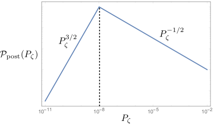
Figure 1: The schematic summary of the probability distribution $\mathcal{P}_{\rm post}(P_{\zeta})$ of having a primordial perturbation amplitude $P_{\zeta}$ from anthropic consideration of post-inflationary evolution.

A spectral index close to unity is apparently challenging. The spectral index $n_{s}$ is given by

$$n_{s}=1+2\eta-6\epsilon,\leavevmode\nobreak\ \eta\equiv\frac{V^{\prime\prime}}{V},\leavevmode\nobreak\ \epsilon\equiv\frac{1}{2}\left(\frac{V^{\prime}}{V}\right)^{2}.$$ (1.5)

Having a spectral index $n_{s}\sim 0.96$ requires $\eta\sim 0.02\ll 1$. In order to explain the nearly-scale-invariant spectrum, we essentially need to solve the $\eta$-problem [34, 35, 36, 37, 38]. It is not obvious if the requirement of the large enough number of e-foldings can ensure such small $\eta$ parameter.

Ref. [39] investigates the distributions of $P_{\zeta}$ and $n_{s}$, assuming that the inflaton potential obeys a Gaussian distribution, and find that the observed values are highly implausible unless the inflaton field value is as large as the Planck scale. Ref. [40] investigates the inflection point inflation also assuming the Gaussian distribution. In this set up the number of the e-folding tends to be larger for a small and positive $\eta$ parameter. After imposing the anthropic requirement, the spectrum tends to be blue, but the probability of $n_{s}<0.97$ is found to be about $0.2$, which is reasonably high. However, the distribution of $P_{\zeta}$ is not discussed.

In this paper we investigate the distributions of $P_{\zeta}$ and $n_{s}$ for a new inflation model where the inflaton is trapped around the origin during the precedent inflation by a Hubble induced mass. Although the field value of the inflaton is homogeneous inside the horizon because of the damping during the precedent inflation, quantum fluctuation of long-wave length modes is produced, which effectively works as a homogeneous but non-zero initial condition of inflation, unless the Hubble induced mass is much larger than the Hubble scale to suppress the quantum fluctuation. We show that this probabilistic nature of inflaton initial condition is an important key to understand $n_{s}$ close to unity. We focus on a supersymmetric model. As we will see, the smallness of $P_{\zeta}$ is then also explained, as some of the parameter of the theory can be biased toward small values or logarithmically distributed in supersymmetric theories. Our results are summarized in Figure 9, where we show the probability distribution $P_{\zeta}\mathcal{P}_{\rm net}(P_{\zeta},k)$ of $P_{\zeta}$ and $k\simeq-\eta$, taking into account of both inflationary and post-inflationary dynamics. In the contour plot we can see that the probability distribution is biased toward smaller $k$ value and hence the $\eta$-problem is solved. In addition, with an anthropic bound on the density contrast $\delta\rho/\rho<\mathcal{O}(10^{-4})$, the observed universe with $P_{\zeta}\sim 10^{-9}$ and $n_{s}\simeq 0.965$, which is marked by the blue star in Figure 9, is actually a typical one.

This paper is organized as follows. In the next section We first elaborate on the necessity of including the probability distribution of inflaton initial condition in generic new inflation models. We then consider a supersymmetric model and parametrize the probability distributions of the couplings. We find that, for a certain distribution of the couplings of the model, the observed small ($P_{\zeta}\sim 10^{-9}$) and scale-invariant $(n_{s}\simeq 0.96)$ curvature perturbation is probabilistically favorable. We then discuss and summarize our results in Sec.3. In the appendix we show our study on the general new-inflation-type model with $Z_{2}$ symmetry, where observed spectral index $n_{s}$ is probabilistically favored but the smallness of primordial perturbation cannot be explained.

2 New Inflation in the Landscape after Quantum Tunneling

In this section we consider new-inflation-type models in the landscape. We assume that the last inflation which explains the flatness of the universe and the observed cosmic perturbation is a new-inflation-type model with an inflaton $\phi$. In the theory with multiple vacua, it is expected that a singlet scalar field $\chi$ stays at its metastable vacuum and drives a precedent inflationary expansion, leading to a homogeneous universe. After the quantum tunneling of the singlet scalar field, the universe becomes an infinite open curvature dominated Friedmann-Robertson-Walker (FRW) universe while the scalar field rolls down to a local minimum with a small potential energy. The universe is eventually dominated by the potential energy of the inflaton (Figure 2). One may naively expect that a coupling between the $\chi$ field and the inflaton (leading to so-called the Hubble induced mass) can trap the inflaton to the origin and the initial inflaton field value $\phi_{i}$ is automatically small enough to initiate the last inflation. This is generically not true. As we will see, after the tunneling the Hubble induced mass of the inflaton is not effective. Therefore the inflaton fluctuation mode that just exited the horizon before quantum tunneling may survive. Although the inflaton field value is homogeneous inside the horizon, the field value must be fine-tuned for the last inflation to occur and last long enough. We investigate the impact of this observation by computing the distribution function of the curvature perturbation $P_{\zeta}$ and the spectral index $n_{s}$ (equivalently the $\eta$ parameter) after requiring enough number of e-folds $\mathcal{N}^{tot}_{e}$ during the last inflation. We find that $P_{\zeta}$ as well as $\eta$ may be biased toward small values, explaining the observed very small ($P_{\zeta}\sim 10^{-9}$) and scale-invariant $(n_{s}\simeq 0.96)$ curvature perturbation.

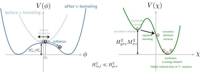
Figure 2: Schematic figure of the proposed scenario.

2.1 Hubble Induced Mass and the Initial Condition after Tunneling

Let us follow the dynamics of the singlet scaler field $\chi$ and the inflaton $\phi$ before the inflation starts. The mass of the inflaton in general depends on the energy density of the universe. Its evolution is summarised in Figure 3.

When the singlet field is at its metastable vacuum $\chi_{\rm pre}$, the potential energy $V_{\chi}$ of the singlet field dominates and the universe is in a precedent inflationary expansion. In the meanwhile, the inflaton acquires a Hubble induced mass and can be driven toward $\phi=0$. For example, in supergravity when the potential energy is dominated by the potential of the moduli field $V_{\chi}$, the potential includes

$$V\supset\frac{V_{\chi}}{M_{*}^{2}}|\phi|^{2},$$ (2.1)

where $M_{*}$ is the cutoff scale. We expect that $V_{\chi}\sim M_{*}^{4}$, and hence the Hubble induced mass of the inflaton, $m_{\phi}(\chi)$, during the precedent inflation is as large as $M_{*}$. The similar is true for non-supersymmetric theories. We expect a coupling of the form

$$M_{*}^{2}f(\frac{\chi}{M_{*}})\phi^{2},$$ (2.2)

where $f$ is some function, leading to the Hubble induced mass of $\mathcal{O}(M_{*})$. The Hubble scale $H_{\rm pre}$ is on the other hand of $\mathcal{O}(M_{*}^{2}/M_{\scriptscriptstyle P\ell})\lesssim M_{*}$. If the Hubble induced mass is positive, the inflaton is driven toward $\phi=0$.

After the quantum tunneling of the singlet field $\chi$ (denoted as $a_{0}$ in Figure 3), the universe is dominated by the curvature energy density $\rho_{K}$ and the singlet field $\chi$ is fixed by the Hubble friction. Because the Hubble induced mass $m_{\phi}^{2}$ is proportional to $\rho_{\chi}$, we have $m^{2}_{\phi}\lesssim H^{2}=\rho_{K}/3M_{\scriptscriptstyle P\ell}^{2}$ right after the tunneling. Note that the curvature energy density alone does not give a Hubble induced mass term. As the universe expands, $\rho_{K}$ decreases and when it becomes smaller than $m_{\chi}^{2}M_{\scriptscriptstyle P\ell}^{2}\sim M_{*}^{2}M_{\scriptscriptstyle P\ell}^{2}$, the singlet field $\chi$ starts to roll down to the global minimum and oscillates. At this point the mass of the inflaton is as large as the Hubble scale. However, since the energy density of the singlet field decreases as $a^{-3}$, the mass of the inflaton $m_{\phi}\sim\rho_{\chi}^{1/2}/M_{\scriptscriptstyle P\ell}$ does not exceed the Hubble scale of the expansion and hence the inflaton can be regarded as massless after the tunneling. When $\rho_{K}$ drops below the inflaton potential energy $H^{2}_{\rm inf}\sim\rho_{\phi}/M_{\scriptscriptstyle P\ell}^{2}$, the inflation begins.

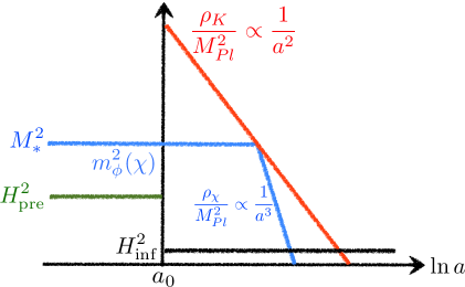
Figure 3: The evolution of inflaton’s Hubble induced mass.

Let us discuss the evolution of the fluctuation of the inflaton based on the above observation. Expanding the field into comoving momentum modes $\phi=\int\frac{d^{3}k}{(2\pi)^{3}}\phi_{\vec{k}}e^{i\vec{k}\cdot\vec{x}}$, the modes fluctuate with decreasing amplitude as the spacetime expands. During the precedent inflation era, after a mode exit the comoving horizon, $k=aH_{\rm pre}$, the amplitude is continually damped because of the Hubble induced mass and eventually vanishes in the superhorizon limit $aH_{\rm pre}\gg k$. Hence, right after tunneling, the superhorizon mode that has the largest amplitude is the one that exited the horizon right before tunneling. This mode has an amplitude

$$\delta\phi_{\rm pre}\simeq H_{\rm pre}\sqrt{\frac{H_{\rm pre}}{m_{\phi}(\chi_{\rm pre})}}\simeq\frac{M_{*}^{5/2}}{M_{\scriptscriptstyle P\ell}^{3/2}}.$$ (2.3)

The horizon after the tunneling resides inside the horizon before the tunneling. The comoving horizon $1/aH$ remains constant during curvature dominant era, and hence there is no horizon entrance nor exit. Thus inflaton fluctuation modes inside the horizon continue to be suppressed, while the long wavelength superhorizon modes are frozen as the inflaton is essentially massless during the curvature dominant era. Those frozen modes effectively work as the zero mode $\phi_{i}$ which obeys a Gaussian distribution with a zero mean and a variance $(\delta\phi_{\rm pre})^{2}$. $\phi_{i}$ is nothing but the initial condition of the new inflation.

In order to wipe out the curvature energy density and to have structures on the galaxy scale, the inflation needs to last long enough with an anthropic bound $\mathcal{N}^{tot}_{e}\gtrsim\mathcal{N}^{\rm ant}_{e}$. In [15], it is found that in order to have typical galaxies being formed, the comoving Hubble scale at the time of photon decoupling should satisfy

$$\frac{a_{dc}H_{dc}}{a_{t}H_{t}}>30,$$ (2.4)

where the subscript $t$ denotes the time right after the quantum tunneling. With some manipulation we have

$$\frac{a_{dc}H_{dc}}{a_{ent}H_{ent}}\frac{a_{*}H_{*}}{a_{end}H_{end}}\frac{a_{end}H_{end}}{a_{i}H_{i}}\frac{a_{i}H_{i}}{a_{t}H_{t}}>30.$$ (2.5)

Here $a_{ent}H_{ent}$ denotes the coving Hubble scale of the horizon re-entrance of the CMB scale, which is equal to that of horizon exit $a_{*}H_{*}$. $a_{end}H_{end}$ and $a_{i}H_{i}$ are the comoving Hubble scales at the end and beginning of the inflation respectively. Because the period between the time right after quantum tunneling and the beginning of inflation is curvature dominant, the comoving Hubble scale remains the same, i.e. $(a_{i}H_{i})/(a_{t}H_{t})$=1. We assume the Hubble scale during the inflation is nearly constant, $H_{i}\simeq H_{*}\simeq H_{end}$. Also, the comoving Hubble scale does not evolve much between the horizon re-entrance of the CMB scale and the photon decoupling, so $(a_{dc}H_{dc})/(a_{ent}H_{ent})\simeq 1$. Putting everything together, we then have a constraint

$$\mathcal{N}^{tot}_{e}>\mathcal{N}^{\rm ant}_{e}\simeq\mathcal{N}^{*}_{e}+3.4\,,$$ (2.6)

where $\mathcal{N}^{*}_{e}$ is the number of e-foldings between the end of the inflation and the horizon exits of the CMB pivot scale.

For potentials of a new inflation type, the initial field value $\phi_{i}$ must be close to zero to have long enough inflation. For a large enough $M_{*}$, $\delta\phi_{\rm pre}$ is larger than the required initial field value and hence some tuning of the initial field value is required. As $\phi_{i}$ obeys a Gaussian distribution, which is flat for small $\phi_{i}$, the probability distribution of $\phi_{i}$ in the region of interest is approximately uniform;

$$\mathcal{P}_{\phi_{i}}d\phi_{i}\propto d\phi_{i}.$$ (2.7)

The anthropic constraint $\mathcal{N}^{tot}_{e}\gtrsim\mathcal{N}^{\rm ant}_{e}$ leads to the upper bound $\phi_{i}<\phi_{\rm ant}$, where $\phi_{\rm ant}$ is the field value of the inflaton such that the number of e-foldings after the inflaton pass the field value is $\mathcal{N}^{\rm ant}_{e}$.

The fact that the initial condition $\phi_{i}$ has a probability distribution over a certain range instead of having to start at $\phi_{i}\simeq 0$ plays an important role to solve the $\eta$-problem in new inflation. Particularly, as now the inflaton tends to start from an initial condition away from zero, the anthropic constraints $\mathcal{N}^{tot}_{e}>\mathcal{N}^{\rm ant}_{e}$ requires the potential around the origin to be flatter. The $\eta$ parameter is biased toward smaller values after the anthropic constraint is imposed. On the contrary, for a small enough $M_{*}$ so that $\phi_{i}\simeq 0$ is forced, then the inflation can easily last longer than $\mathcal{N}^{\rm ant}_{e}$ e-folds and the anthropic constraints on $\mathcal{N}^{tot}_{e}$ plays no significant role. We will see this point quantitatively in the following.

2.2 A Supersymmetric New Inflation Model

In the appendix we study a new inflation model with $Z_{2}$ symmetry, assuming that the parameters of the potential are uniformly distributed. We find that the resultant $P_{\zeta}$ is strongly biased toward a large value, and the observed one is probabilistically disfavored. Here we in stead investigate a supersymmetric model where it is sensible that the parameters of the model, including the scale of the inflation, obey distributions different from uniform ones. We expect that for certain distributions of the parameters, $P_{\zeta}$ is biased toward small ones. In particular, we consider an $R$-symmetric single field new inflation model [42, 43, 44] with a discrete $R$-symmetry $Z_{2N}$ is present and the superpotential

$$W=v^{2}\Phi-\frac{g}{N+1}\Phi^{N+1},$$ (2.8)

where $\Phi$ is a chiral superfield while $v$ and $g$ are constants. Here and here after, we work in the unit where the reduced Planck scale is unity. The Kähler potential is

$$K=\Phi^{\dagger}\Phi+\frac{1}{4}k(\Phi^{\dagger}\Phi)^{2}\cdots,$$ (2.9)

where the ellipses denote higher order terms that are irrelevant to the inflationary dynamics. From Eqs.(2.8) and (2.9), the potential of the scalar component of $\Phi$ which we call $\varphi$ is given by

$$V(\varphi) =|v^{2}-g\varphi^{N}|^{2}-kv^{4}|\varphi|^{2}+\cdots$$

$$=v^{4}-kv^{4}|\varphi|^{2}-\big{(}gv^{2}\varphi^{N}+\text{ h.c.}\big{)}+\cdots.$$ (2.10)

In terms of the radial and angular components, $\varphi=\frac{\phi}{\sqrt{2}}e^{i\theta}$, the potential can be rewritten as

$$V=v^{4}-\frac{1}{2}kv^{4}\phi^{2}-\frac{g}{2^{\frac{N-2}{2}}}v^{2}\phi^{N}\cos(N\theta).$$ (2.11)

For simplicity we assume that the inflaton has an initial condition around $\theta=0$ mod $2\pi/N$ (which are minima along the angular direction) and focus only on the radial direction.

In the appendix we study general new-inflation-type models with $Z_{2}$ symmetry. Here the resulting potential has the form of Eq.(B.2) without the $c_{m}$ perturbation term. Using Eqs.(B.9) and (B.10) with $a=v^{4}$, $b=kv^{4}$, $c_{n}=gv^{2}/2^{(N-2)/2}$ and $c_{m}=0$, we have

$$n_{s}\simeq 1-2k-2N(N-1)kf_{\scriptscriptstyle N}^{*}\quad,$$ (2.12)

$$P_{\zeta}=\frac{\Big{[}g^{2}v^{4(N-3)}k^{-2(N-1)}{f_{\scriptscriptstyle N}^{*}}^{-2}\Big{]}^{\frac{1}{N-2}}}{24\pi^{2}\left(1+Nf_{\scriptscriptstyle N}^{*}\right)^{2}},$$ (2.13)

where

$$f_{\scriptscriptstyle N}\equiv f_{\scriptscriptstyle N}(k,\mathcal{N}_{e})=\frac{1}{N}\frac{1}{\left(\left[1+(N-1)k\right]e^{(N-2)k\mathcal{N}_{e}}-1\right)}$$ (2.14)

and $f_{\scriptscriptstyle N}^{*}=f_{\scriptscriptstyle N}(k,\mathcal{N}_{e}^{*})$ in which $\mathcal{N}^{*}_{e}$ is the number of e-folds between the horizon-exit of the CMB scale and the end of inflation.

The spectral index $n_{s}$, as given in Eq.(2.12), is a function of the parameter $k$, and the number of e-folds $\mathcal{N}^{*}_{e}$ between the horizon exit of the CMB scale and the end of inflation. Assuming instant reheating, this is determined by the inflation energy scale,

$$\mathcal{N}^{*}_{e}\simeq 62+\ln\left(\frac{v}{M_{\scriptscriptstyle P\ell}}\right).$$ (2.15)

Using Eq.(2.13) with $k=0.01$ and the observed $P_{\zeta}$ to get an estimate on $v$, we have $\mathcal{N}^{*}_{e}\simeq 52$. Setting $\mathcal{N}^{*}_{e}=52$, we plot the spectral index $n_{s}$ as a function of $k$ in Figure 4. One can see that $N=4$ and 5 are ruled out by the observation, while $N=6$ fits the observation very well in a certain region of $k$. Even if we relax the assumption of instant reheating, such that $\mathcal{N}^{*}_{e}<52$, the maximum $n_{s}(k)$ of $N=6$ case lies in the observational allowed region unless the reheating temperature is very small. In below we frequently use $N=6$, i.e. the model with discrete $Z_{12}$ $R$-symmetry, as a reference point.

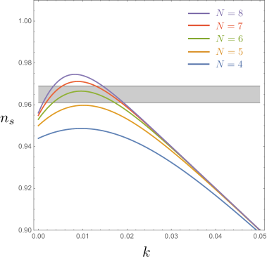
Figure 4: The $n_{s}-k$ plot for $N=4,5,6,7$ and 8, with $\mathcal{N}^{*}_{e}=52$.

2.3 Probability Distribution of the Observables

A natural question now arises: what is the probability for $k$ to lie in the region that yields observationally allowed $n_{s}$? From Figure 4 we see that the observed $n_{s}$ requires $k$ to be of the order of 0.01, while in general $k$ would be much larger. Note that the slow-roll parameter $\eta$ is related to $k$ by $\eta=-k$. Therefore, making the observed spectral index $n_{s}\sim 0.96$ probabilistically favorable is equivalent to solving the $\eta$-problem, and this requires a probability distribution that biases toward small $k$.

To investigate the probability distribution function of the observables, we need to first make assumptions on the probability distribution of the Lagrangian parameters. As $k$ is a coupling in the Kähler potential, it would be natural that $k$ obeys a uniform probability distribution $\mathcal{P}(k)dk\propto dk$. The parameters $v^{2}$ and $g$ are superpotential couplings and may obey distributions different from uniform ones. Furthermore, those parameters are related with the vacuum expectation value (vev) of the superpotential $W_{0}\equiv\left\langle{W}\right\rangle\sim v^{2(1+1/N)}g^{-1/N}$, which is related with the electroweak scale and the cosmological constant. Let us start from the distribution of $v^{2}$, $g$, the supersymmetry breaking scale $F$ and the $\mu$ term of the electroweak Higgs,

$$dv^{2}v^{2p^{\prime}}\times dgg^{q^{\prime}}\times dFF^{r}\times d\mu\mu^{s}.$$ (2.16)

If a parameter is given by a dimensional transmutation, the index ($p^{\prime},q^{\prime},r,s$) of the distribution is $-1$, while it is $1$ if the parameter is a complex parameter biased toward a large value. The electroweak scale $v_{\rm EW}^{2}$ is given by

$$v_{\rm EW}^{2}\simeq F^{2}/M_{\rm med}^{2}-\mu^{2},$$ (2.17)

where $M_{\rm med}$ is the mediation scale of the supersymmetry breaking. We assume that the electroweak scale must be in a certain range close to the observed one as is argued in [45, 46],

$$cv_{\rm EW,obs}^{2}<v_{\rm EW}^{2}<c^{\prime}v_{\rm EW,obs}^{2},$$ (2.18)

where $c$ and $c^{\prime}$ are constants which we do not have to specify. The scanning over the $\mu$ parameter yields

$$\int_{cv_{\rm EW,obs}^{2}<v_{\rm EW}^{2}<c^{\prime}v_{\rm EW,obs}^{2}}d\mu\mu^{s}\simeq v_{\rm EW,obs}^{2}\left(\frac{F}{M_{\rm med}}\right)^{s-1}\propto F^{s-1},$$ (2.19)

where we have used $F/M_{\rm med}\simeq\mu\gg v_{\rm EW,obs}$ as is suggested by the non-discovery of supersymmetric particles so far. The cosmological constant is given by

$$\rho_{\Lambda}=F^{2}-3W_{0}^{2}M_{\scriptscriptstyle P\ell}^{2},$$ (2.20)

where $W_{0}$ is the vev of the superpotential. A change of variables gives gives

$$\int dFF^{r+s-1}\propto W_{0}^{r+s-2}d\rho_{\Lambda}.$$ (2.21)

Here we have used $F^{2}\simeq 3W_{0}^{2}M_{\scriptscriptstyle P\ell}^{2}\gg\rho_{\Lambda}$. We omit the measure $d\rho_{\Lambda}$, which leads to the uniform distribution of the cosmological constant, in the following. Using the relation $W_{0}\sim v^{2(1+1/N)}g^{-1/N}$, the distribution of $v^{2}$ and $g$ are given by

$$dv^{2}v^{2p}\times dgg^{q},\leavevmode\nobreak\ \leavevmode\nobreak\ p=p^{\prime}+(1+\frac{1}{N})(r+s-2),\leavevmode\nobreak\ \leavevmode\nobreak\ q=q^{\prime}-\frac{1}{N}(r+s-2).$$ (2.22)

For $-1\leq p^{\prime},q^{\prime},r,s\leq 1$, a wide range of $(p,q)$ can be obtained.

Putting everything together, the probability distribution of the parameters to start with is

$$\int d\phi_{i}\,dk\,dg\,\,dv^{2}\,\,g^{q}\,v^{2p}.$$ (2.23)

The distribution of the initial condition $\phi_{i}$ is uniform as discussed in Sec.2.1. If the anthropic bound $\phi_{\rm ant}$ is smaller than the amplitude of quantum fluctuation $\delta\phi_{\rm pre}$ given by Eq.(2.3), then the integration of $d\phi_{i}$ ranges from $0$ to $\phi_{\rm ant}$. On the other hand, if $\phi_{\rm ant}>\delta\phi_{\rm pre}$, the integration of $d\phi_{i}$ is capped by $\delta\phi_{\rm pre}$ and the anthropic constraint is no longer effective. In other words, integrating out $d\phi_{i}$ yields

$$\int\,dk\,dg\,\,dv^{2}\,\,g^{q}\,v^{2p}\phi_{\rm bound},\leavevmode\nobreak\ \leavevmode\nobreak\ \leavevmode\nobreak\ \phi_{\rm bound}\equiv\min[\phi_{\rm ant},\delta\phi_{\rm pre}].$$ (2.24)

Using Eqs.(B.6), (B.11) and (2.13), the field value $\phi_{\rm ant}$ is given by

$$\phi_{\rm ant} =\sqrt{2}\,g^{-\frac{1}{N-3}}k^{\frac{2}{N-3}}{f_{\scriptscriptstyle N}^{*}}^{\frac{1}{(N-3)(N-2)}}\left[24\pi^{2}\left(1+Nf_{\scriptscriptstyle N}^{*}\right)^{2}\right]^{\frac{1}{2(N-3)}}{f_{\scriptscriptstyle N}^{\rm ant}}^{\frac{1}{N-2}}P_{\zeta}^{\frac{1}{2(N-3)}}$$

$$=\sqrt{2}g^{-\frac{1}{N-3}}{f_{\scriptscriptstyle N}^{\rm ant}}^{\frac{1}{N-2}}k^{\frac{1}{N-2}}h^{\frac{1}{(N-3)(N-2)}}P_{\zeta}^{\frac{1}{2(N-3)}},$$ (2.25)

where we have defined

$$h(k)\equiv k^{N-1}f_{\scriptscriptstyle N}^{*}\left[24\pi^{2}(1+Nf_{\scriptscriptstyle N}^{*})^{2}\right]^{\frac{N-2}{2}}$$ (2.26)

for future convenience. It is instructive to understand the behavior of $h(k)$ and the contribution of $\phi_{\rm ant}$, if $\phi_{\rm ant}<\delta\phi_{\rm pre}$, to the final probability distribution of $k$ which we plot in Figure 5. Most importantly, we can see that $\phi_{\rm ant}$ gives a bias toward small $k$, which is the key of solving the $\eta$-problem and making observed spectral index $n_{s}$ probabilistically favorable.

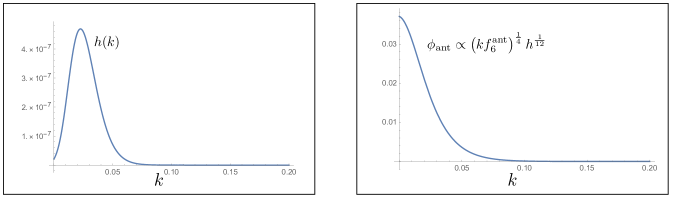
Figure 5: The function $h(k)$ (left) and the contribution of $\phi_{\rm ant}$ to the probability distribution of $k$ (right). We take $N=6$ and $\mathcal{N}^{*}_{e}=52$.

Using the relation between $v^{2}$ and $P_{\zeta}$ derived from Eq.(2.13),

$$v^{2}=g^{-\frac{1}{N-3}}h^{\frac{1}{N-3}}P_{\zeta}^{\frac{N-2}{2(N-3)}},$$ (2.27)

we can perform a change of variable to obtain the probability distribution in terms of cosmic perturbation $P_{\zeta}$. For the parameter region where $\phi_{\rm ant}<\delta\phi_{\rm pre}$, we have

$$\int\,dk\,dg\,\,dv^{2}\,\,g^{q}\,v^{2p}\phi_{\rm ant}$$ (2.28)

$$= \frac{(N-2)}{\sqrt{2}(N-3)}\int dk\,\frac{dP_{\zeta}}{P_{\zeta}}\,dg\,g^{\frac{q(N-3)-p-2}{N-3}}h^{\frac{(p+1)}{(N-3)}}P_{\zeta}^{\frac{(N-2)(p+1)}{2(N-3)}}\left[\left(kf_{\scriptscriptstyle N}^{\rm ant}\right)^{\frac{1}{N-2}}h^{\frac{1}{(N-3)(N-2)}}P_{\zeta}^{\frac{1}{2(N-3)}}\right],$$ (2.29)

where we have left the contribution from $\phi_{\rm ant}$ to $k$- and $P_{\zeta}$-distribution in the square brackets for future convenience. We now need to integrate out $g$ to obtain the final probability distribution. When $q(N-3)-p+N-5\neq 0$, the integration yields

$$\frac{(N-2)}{\sqrt{2}\left[q(N-3)-p+N-5\right]}\int dk\,\frac{dP_{\zeta}}{P_{\zeta}}\left[g^{\frac{q(N-3)-p+N-5}{(N-3)}}\right]^{g_{max}}_{g_{min}}h^{\frac{(p+1)}{(N-3)}}P_{\zeta}^{\frac{(N-2)(p+1)}{2(N-3)}}\Big{[}\cdots\Big{]}$$ (2.30)

where the ellipses in the square brackets represent the contribution from $\phi_{\rm ant}$ as in Eq.(2.29). The lower cutoff of the integral $g_{min}$ is given by Eq.(2.27) with the natural requirement $v^{2}\leq M_{*}^{2}$, i.e. the energy scale $v$ should not be larger than the cut off scale. Particularly, we have

$$g_{min}=hP_{\zeta}^{\frac{N-2}{2}}M_{*}^{-(N-3)}\ll 1.$$ (2.31)

On the other hand, $g_{max}$ is determined by the cutoff scale $M_{*}$. After restoring $M_{\scriptscriptstyle P\ell}$ and $M_{*}$ to the superpotential, we have

$$W\supset-\frac{1}{N+1}\frac{g}{M_{\scriptscriptstyle P\ell}^{N-2}}\Phi^{N+1}\equiv-\frac{1}{N+1}\frac{c_{g}}{M_{*}^{N-2}}\Phi^{N+1}.$$ (2.32)

Assuming the dimensionless coupling $c_{g}$ is bounded by unity, the coupling $g$ is bounded by

$$g<g_{max}=\left(\frac{M_{\scriptscriptstyle P\ell}}{M_{*}}\right)^{N-2}.$$ (2.33)

Therefore, if $q(N-3)-p+N-5>0$, the $g-$integration merely gives a proportional constant and does not affect the probability distribution of $k$ and $P_{\zeta}$. We therefore have

$$\mathcal{P}_{\rm inf}(k,P_{\zeta})dk\,dP_{\zeta}=\mathcal{P}_{k}\mathcal{P}_{P_{\zeta}}dk\,dP_{\zeta}=\mathcal{P}_{k}P_{\zeta}\mathcal{P}_{P_{\zeta}}dk\,d{\rm ln}P_{\zeta}$$ (2.34)

where $\mathcal{P}_{\rm inf}$ is the probability distribution from inflationary dynamics with

$$\mathcal{P}_{k} \propto h^{\frac{(p+1)}{(N-3)}}\left[\left(kf_{\scriptscriptstyle N}^{60}\right)^{\frac{1}{N-2}}h^{\frac{1}{(N-3)(N-2)}}\right],$$ (2.35)

$$P_{\zeta}\mathcal{P}_{P_{\zeta}} \propto P_{\zeta}^{\frac{(N-2)(p+1)}{2(N-3)}}P_{\zeta}^{\frac{1}{2(N-3)}}.$$ (2.36)

The quantity $P_{\zeta}\mathcal{P}_{P_{\zeta}}$ can be understood as the relative probability to obtain the curvature perturbation of $\mathcal{O}({\cal P}_{\zeta})$. When $q(N-3)-p+N-5=0$, Eq.(2.30) does not apply and the integration over $g$ yields a logarithmic contribution $\ln(g_{min})$ instead. This logarithmic contribution changes the probability distribution of $k$ and $P_{\zeta}$ only slightly, and we may use Eqs.(2.35) and (2.36) as a good approximation.

If $\phi_{\rm ant}>\delta\phi_{\rm pre}$, then $\phi_{\rm ant}$ plays no role and the integration of $\phi_{i}$ and $g$ merely yields a proportional constant which do not affect the probability distribution of the observables:

$$\int\,dk\,dg\,\,dv^{2}\,\,g^{q}\,v^{2p}\phi_{\rm bound}\propto\int dk\,\frac{dP_{\zeta}}{P_{\zeta}}h^{\frac{(p+1)}{(N-3)}}P_{\zeta}^{\frac{(N-2)(p+1)}{2(N-3)}}.$$ (2.37)

Thus for $\phi_{\rm ant}>\delta\phi_{\rm pre}$, we obtain

$$\mathcal{P}_{k} \propto h^{\frac{(p+1)}{(N-3)}},$$ (2.38)

$$P_{\zeta}\mathcal{P}_{P_{\zeta}} \propto P_{\zeta}^{\frac{(N-2)(p+1)}{2(N-3)}}.$$ (2.39)

Note that in the parameter region $q(N-3)-p+N-5\geq 0$, the probability distribution is parametrized only by $p$ but not by $q$.

In the parameter region where $q(N-3)-p+N-5<0$, the integration over $g$ is dominated by the lower cutoff contribution, where $g=g_{min}\ll 1$. Recall that $\phi_{ant}\propto g^{-1/(N-3)}$, and hence for such a small $g$, $\phi_{ant}$ is much larger than $M_{\scriptscriptstyle P\ell}$. This means the inflaton field value at the CMB scale will also be much larger than $M_{\scriptscriptstyle P\ell}$, and therefore the assumption of small field inflation breaks down.

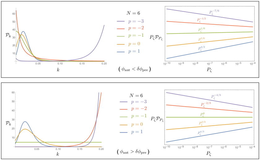
Figure 6: The probability distribution functions in the parameter region $q(N-3)-p+N-5\geq 0$ when $\phi_{\rm ant}<\delta\phi_{\rm pre}$ (upper panel) and $\phi_{\rm ant}>\delta\phi_{\rm pre}$ (lower panel), respectively. We take $N=6$ and $\mathcal{N}^{*}_{e}=52$.

In Figure 6 we plot the distribution function using Eqs.(2.35), (2.36), (2.38) and (2.39) in the parameter region $q(N-3)-p+N-5\geq 0$ for both $\phi_{\rm ant}<\delta\phi_{\rm pre}$ and $\phi_{\rm ant}>\delta\phi_{\rm pre}$. Let us first look at the upper left panel of Figure 6. We see that $\mathcal{P}_{k}$ is largely suppressed for large $k$ as long as $p\geq-2$. To understand how the parameter $p$ alters the probability distribution at large $k$, note that the functions $f_{\scriptscriptstyle N}$ and $h$ behave as

$$f_{\scriptscriptstyle N} \propto k^{-1}e^{-(N-2)k\mathcal{N}_{e}}$$ (2.40)

$$h \propto k^{N-2}e^{-(N-2)k\mathcal{N}_{e}}$$ (2.41)

when $k\to\infty$, and hence

$$\mathcal{P}_{k}\propto k^{\frac{(N-2)(p+1)+1}{N-3}}e^{-\frac{(N-2)(p+2)}{N-3}k\mathcal{N}_{e}}$$ (2.42)

for large $k$. It is therefore clear that in order to solve the $\eta$-problem, one requires $p\geq-2$ so that the distribution is suppressed for large $k$.

The behavior of $\mathcal{P}_{k}$ for negative $p$ can be understood as follows. Recall that the primordial perturbation is given as

$$P_{\zeta}\sim\frac{V}{\epsilon}\sim\frac{v^{4}}{k^{2}\phi^{2}_{\rm cmb}}.$$ (2.43)

where $\phi_{\rm cmb}$ is the inflaton field value when the CMB scale exited the horizon. Therefore, for a fixed $P_{\zeta}$, smaller $v^{2}$ requires smaller $k\phi_{\rm cmb}$. For a given e-folds $\mathcal{N}^{*}_{e}$, the field value $\phi_{\rm cmb}$ is in fact related to the parameter $k$. For larger $k$, the potential is steeper and hence $\phi_{\rm cmb}$ has to be smaller to maintain the same number of e-folds. (This relation is explicitly shown in Figure 13 in the appendix.) The full $k$-dependence of the denominator $k^{2}\phi^{2}_{\rm cmb}(k)$ is thus nontrivial, and is worked out in Eq.(B.6). It turns out that when $k$ decreases, $k^{2}\phi^{2}_{\rm cmb}(k)$ increases. Therefore, for a given $P_{\zeta}$, if $v^{2}$ is biased toward small values as when $p$ is negative, then $k$ is biased toward large values. This is why large $k$ is favored when $p$ is too negative, where the bias toward small $k$ from $\phi_{\rm ant}$ is defeated.

So far we have only discussed the probability distribution in terms of $k$ but not the observable $n_{s}$. Since the spectral index $n_{s}$ is a function of $k$ only, as given in Eq.(2.12), the probability distribution of $k$ is sufficient to give the probabilistic information of $n_{s}$. That being said, the probability distribution of $n_{s}$ displays an important feature of $R$-symmetry new inflation which we now discuss. To this end, we perform a change of variable from $k$ to $n_{s}$,

$$\int dk\,\mathcal{P}_{k}=\int dn_{s}\left|\frac{\partial k}{\partial n_{s}}\right|\mathcal{P}_{k}(k(n_{s}))\equiv\int dn_{s}\,\mathcal{P}_{n_{s}}.$$ (2.44)

As shown in Figure 4, the function $n_{s}(k)$ is not monotonic and has a maximum $n^{max}_{s}$ very close to the observed value $n_{s}\simeq 0.965$. These two properties have important implications in $\mathcal{P}_{n_{s}}$ we show in Figure 7. The first feature of $\mathcal{P}_{n_{s}}$ is the jump due to non-monotonicity of $n_{s}(k)$. The second, and probably more important, feature of $\mathcal{P}_{n_{s}}$ is that $n_{s}$ will never reach $n_{s}=1$ and $\mathcal{P}_{n_{s}}$ diverges at $n^{max}_{s}$ because the Jacobian factor $\left|\frac{\partial k}{\partial n_{s}}\right|$ diverges at $n^{max}_{s}$. Once the probability distribution of large $k$ ($n_{s}\ll 1$) is suppressed due to the probabilistic nature of initial field value $\phi_{i}$, in $R$-symmetry new inflation we not only can explain why $n_{s}$ is very close to one, but can also predict an $n_{s}\neq 1$ that is near the observed value $n_{s}\simeq 0.965$. For $\mathcal{N}^{*}_{e}=52$ and $p=-1$, the probability for $0.96<n_{s}<n^{max}_{s}$ is

$$P_{0.96<n_{s}<n^{max}_{s}}=\frac{\displaystyle\int^{n^{max}_{s}}_{0.96}\,\mathcal{P}_{n_{s}}\,dn_{s}}{\displaystyle\int^{n^{max}_{s}}_{-\infty}\,\mathcal{P}_{n_{s}}\,dn_{s}}\simeq 0.48\,,$$ (2.45)

and the probability distribution diverges at $n_{s}^{max}\simeq 0.966$. Note that $p=-2$ yields a similar result.

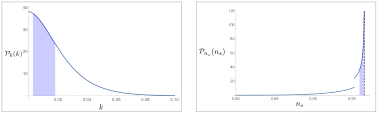
Figure 7: The normalized probability distribution function for $k$ (left) and $n_{s}$ (right). The shaded areas corresponds to the parameter region where $n_{s}>0.96$.

Move on to the probability distribution of $P_{\zeta}$, the upper right panel of Figure 6 shows that $P_{\zeta}$ is biased toward smaller values for a sufficiently negative $p$. This is simply because $P_{\zeta}$ is proportional to the inflation scale, and hence a bias toward small $v^{2}$ results in a bias toward small $P_{\zeta}$. For $p=-2$, the perturbation $P_{\zeta}$ is biased toward small value strongly. For $p=-1$, $P_{\zeta}$ is biased toward large values only mildly. The power of $P_{\zeta}\mathcal{P}_{P_{\zeta}}$, as shown in Eq.(2.36), is given by

$$\frac{p(N-2)+(N-1)}{2(N-3)}=\frac{(p+2)(N-2)}{2(N-3)}-\frac{1}{2}.$$ (2.46)

In order to solve the $\eta$-problem simultaneously, we need $p\geq-2$. The most negative power we can get for the probability of $P_{\zeta}$ from inflationary dynamics is then $-1/2$.

As we mentioned in the introduction, the anthropic consideration on the post-inflation dynamics gives an additional bias on $P_{\zeta}\mathcal{P}_{P_{\zeta}}$ that scales as $P_{\zeta}^{3/2}$ for small $P_{\zeta}$, and scales as $P_{\zeta}^{-1/2}$ for large $P_{\zeta}$ where the turning point is at $P_{\zeta}\sim 10^{-8}$. See Figure 1. Combining this with the contribution from inflationary evolution, we see that the power of $P_{\zeta}\mathcal{P}_{P_{\zeta}}$ should be smaller or equal to $\frac{1}{2}$, since otherwise $P_{\zeta}\sim O(1)$ is much more favored than $P_{\zeta}\sim 10^{-9}$. This requires

$$p\leq\frac{-2}{N-2}.$$ (2.47)

Recall that in order to solve the $\eta$-problem, one requires $p\geq-2$. Hence, to simultaneously solve the $\eta$-problem and explain the smallness of perturbation power spectrum, we need

$$-2\leq p\leq\frac{-2}{N-2}.$$ (2.48)

The probability to obtain the observed value $P_{\zeta}\simeq 2.1\times 10^{-9}$ is maximized when $p=-2$: With an anthropic bound on the density contrast $\delta\rho/\rho<\mathcal{O}(10^{-4})$ from the property of galaxies, the probability is $O(10)$%, which is reasonable.

To show the impact of the bias from $\phi_{\rm ant}$, in the lower panel of Figure 6, we show the distribution functions without the $\phi_{\rm ant}$ contribution originated from the probabilistic nature of the initial field value $\phi_{i}$, which is the case when $\phi_{\rm ant}>\delta\phi_{\rm pre}$. Comparing with the upper panel, we see that this does not affect the distribution of $P_{\zeta}$ much. However, for the distribution of $k$, the probability for large $k$ is suppressed only for $p=0$ and 1. For $p=-1$, without the additional suppression at large $k$ from $\phi_{\rm ant}$ as illustrated in the right figure of Figure 5, we have a uniform distribution in $k$ and hence it is more likely to find $k$ to be of order 1, instead of order 0.01. Comparing both distributions in the lower panel of Figure 6, it is clear that without scanning the initial condition $\phi_{i}$, it is impossible to simultaneously solve the $\eta$-problem and explain the smallness of $P_{\zeta}$.

We summarize the discussion of the $(p,q)$ parameter space for $N=6$ in Figure 8. The gray-shaded region is where $q(N-3)-p+N-5<0$ and the small field assumption breaks down; the red region is where the probability distribution of $P_{\zeta}$ biases toward large value even though the parameter $k$ tends to be small; the orange region is the opposite, where the $\eta$-problem persists despite the smallness of the perturbation power spectrum can be explained. In between the two regions we have parameter sets that can solve both problems. Those values of $(p,q)$ can be obtained by appropriate choice of $(p^{\prime},q^{\prime},r,s)$.

In claiming the existence of viable $(p,q)$, we assume the contribution to the distribution of $P_{\zeta}$ from the post-inflationary dynamics shown in Figure 1. If the power of the distribution at large $P_{\zeta}$ increases/decreases because of possible biases we have not considered, the white region in Figure 8 shrinks/expands. The white region exists as long as the power is smaller than $1/2$.

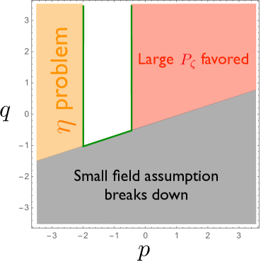
Figure 8: Illustration of the result in $(p,q)$ parameter space for $N=6$. The white region represents the parameter space where both the $\eta$-problem and the smallness of cosmic perturbation can be explained.

It is worth emphasizing again that the viable parameter sets, the white region in Figure 8, exists because of the probabilistic nature of the inflaton initial field value $\phi_{i}$. Without this contribution, the window between the red and orange regions is closed. We examine in which part of the parameter space is $\phi_{\rm ant}<\delta\phi_{\rm pre}$ and does the contribution of $\phi_{\rm ant}$ kick in. Recall that the amplitude of the quantum fluctuation $\delta\phi_{\rm pre}$ is proportional to $M_{*}^{5/2}$ as given in Eq.(2.3). On the other hand, $\phi_{\rm ant}$ also depends on $M_{*}$ through the superpotential coupling $g$. The probability distribution then has the form

$$\int\,dk\,dg\,\,dv^{2}\,\,g^{q}\,v^{2p}\,\phi_{\rm bound}(k,P_{\zeta},g;M_{*})$$

$$= \frac{(N-2)}{\sqrt{2}(N-3)}\int dk\,\frac{dP_{\zeta}}{P_{\zeta}}\,dg\,g^{\frac{q(N-3)-p-1}{N-3}}h^{\frac{(p+1)}{(N-3)}}P_{\zeta}^{\frac{(N-2)(p+1)}{2(N-3)}}\phi_{\rm bound}(k,P_{\zeta},g;M_{*}).$$ (2.49)

The parameter region of interest is $q(N-3)-p+N-5>0$. Therefore after integrating out $g$, the integration is dominated by $g_{max}=(M_{\scriptscriptstyle P\ell}/M_{*})^{N-2}$, at which

$$\phi_{\rm bound}(k,P_{\zeta};M_{*})=\min\big{[}\phi_{\rm ant}(k,P_{\zeta},g_{max}),\delta\phi_{\rm pre}\big{]}.$$ (2.50)

Combining with the contribution from the anthropic constraint discussed in the introduction,

$$\mathcal{P}_{\rm post}\left({P_{\zeta}}\right)=\min\left[(P_{\zeta}/10^{-8})^{3/2},(P_{\zeta}/10^{-8})^{-1/2}\right],$$ (2.51)

the net probability distribution $P_{\zeta}\mathcal{P}_{\rm net}(k,P_{\zeta})$ in the $(k,P_{\zeta})$ space that includes both inflationary and post-inflationary dynamics is proportional to

$$h^{\frac{(p+1)}{(N-3)}}P_{\zeta}^{\frac{(N-2)(p+1)}{2(N-3)}}\min\big{[}\phi_{\rm ant}(k,P_{\zeta},g_{max}),\delta\phi_{\rm pre}\big{]}\min\left[(P_{\zeta}/10^{-8})^{3/2},(P_{\zeta}/10^{-8})^{-1/2}\right].$$ (2.52)

The distribution $P_{\zeta}\mathcal{P}_{\rm net}$ normalized with respect to $P_{\zeta}\mathcal{P}_{\rm net}\big{|}_{k_{obs},P_{\zeta}^{obs}}$ for $N=6$, $p=-2$ and $M_{*}=10^{-2}M_{\scriptscriptstyle P\ell}$ is given in the left panel of Figure 9, where $k_{obs}\simeq 0.0134$ and $P_{\zeta}^{obs}\simeq 2.2\times 10^{-9}$ are the observed value for the parameter $k$ and the cosmic perturbation $P_{\zeta}$ respectively and $(k_{obs},P_{\zeta}^{obs})$ is marked by the blue star. To the right of the blue dashed line, $\phi_{\rm ant}<\delta\phi_{\rm pre}$ and the anthropic constraints $\phi_{\rm ant}$ plays an important role to solve the $\eta$-problem. The observed point $(k_{obs},P_{\zeta}^{obs})$ lies deep inside the region and hence the proposed scenario can indeed explain the nearly scale invariant small cosmic perturbation. Note that the cusps at $P_{\zeta}\sim 10^{-8}$ originate from the turning point of $\mathcal{P}_{\rm post}(P_{\zeta})$, while the cusps at the blue dashed line are due to $\min\big{[}\phi_{\rm ant}(k,P_{\zeta},g_{max}),\delta\phi_{\rm pre}\big{]}$. The distribution for $M_{*}=10^{-1}M_{\scriptscriptstyle P\ell}$ is given in the right panel, where the blue dashed line is absent because $\delta\phi_{\rm pre}\propto M_{*}^{5/2}$ is always larger than $\phi_{\rm ant}$.

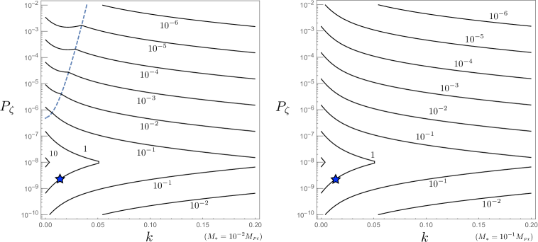
Figure 9: The contour plot of $\frac{P_{\zeta}\mathcal{P}_{\rm net}(k,P_{\zeta})}{P_{\zeta}\mathcal{P}_{\rm net}\big{|}_{k_{obs},P_{\zeta}^{obs}}}$ for $N=6$, $p=-2$ and $M_{*}=10^{-2}M_{\scriptscriptstyle P\ell}$ ($M_{*}=10^{-1}M_{\scriptscriptstyle P\ell}$) on the left (right). To the right of the blue dashed line, $\phi_{\rm ant}<\delta\phi_{\rm pre}$ and hence the anthropic constraints $\phi_{i}<\phi_{\rm ant}$ contributes to the probability distribution. The blue star marks the point $(k_{obs},P_{\zeta}^{obs})$

3 Summary and Discussion

In this work we have investigated the typicality of the small and nearly scale-invariant perturbation in the landscape. Anthropic consideration of the cosmological constant yields a probability of $P_{\zeta}$ that biases toward large perturbation, until the anthropic constraint due to the density of the galaxy kicks in. In order for the observed small $P_{\zeta}\sim 10^{-9}$ to be typical, the inflationary evolution has to give a bias toward small $P_{\zeta}$. Closeness of the spectral index to the unity should be also explained.

We consider the following scenario that naturally fits into the landscape scenario: The inflaton is coupled to a singlet scalar field that was initially trapped in a metastable vacuum and drove a precedent inflation. After the quantum tunneling of the singlet field, the universe became an open FRW universe dominated by the curvature energy density while the singlet field rolled down to a stable vacuum with negligible energy density. After a sufficient period of cosmic expansion, when the curvature energy density dropped below the potential energy of the inflaton, the inflation which explains the flatness of the universe and the cosmic perturbation occurred.

In this scenario, the inflaton field value is homogeneous inside the horizon because of the trapping during the precedent inflation. However, after the quantum tunneling the universe is curvature dominated and the trapping is no longer effective. As a result quantum fluctuation of long wavelength modes produced during the precedent inflation survive, which leads to a probabilistic nature of the initial field value of the inflaton. As the inflaton tends to start from the an initial condition away from the origin, the anthropic lower bound on the total number of e-folding during inflation favors the inflaton potential flatter around the origin, namely a smaller $\eta$ parameter.

We investigated a supersymmetric new inflation model in detail. We find that for certain distributions of the parameters, the probability to obtain $P_{\zeta}\sim 10^{-9}$ is $\mathcal{O}(10)$%, while the observed $n_{s}$ is favored. We emphasize that both the model-building and the anthropic selection from the landscape play important roles in explaining the observed properties of the cosmic perturbation, $P_{\zeta}$ and $n_{s}-1$. From the model-building side, the distribution function of the model parameters, which is not uniform owing to the supersymmetry and the $R$ symmetry, yields the distribution of $P_{\zeta}$ not biased toward large values. From the landscape side, the requirement of large enough number of e-foldings and the probabilistic nature of the initial inflaton field value set by the precedent inflation dynamics favor small $\eta$ parameter, thereby explaining the observed $n_{s}$.

The result is encouraging for the project on understanding the universe by the anthropic principle in the landscape. Further study is required toward this goal. For instance, in this paper we assume the contribution to the distribution of $P_{\zeta}$ from the post-inflationary dynamics shown in Figure 1. As we comment in Sec. 2.3, our result holds qualitatively as long as the power of the distribution at large $P_{\zeta}$ is smaller than $1/2$. It will be important to investigate the distribution at large $P_{\zeta}$ more carefully, taking into account the effect of e.g. the behavior of proto-galaxies.

Appendix A Fine-tuning in General New Inflation

In the appendix we study fine-tuning problems in general new-inflation-type models. The only symmetry we impose here is $Z_{2}$ symmetry, where the most generic potential is of the form

$$V(\phi)=M_{\scriptscriptstyle P\ell}^{4}\left[V_{0}+\sum_{n=1}^{\infty}c_{\scriptscriptstyle 2n}\left(\frac{\phi}{M_{\scriptscriptstyle P\ell}}\right)^{2n}\right].$$ (A.1)

Hereafter we will work in the Planck unit where the reduced Planck mass $M_{\scriptscriptstyle P\ell}$ is set to unity. We study how much fine-tuning is required to yield the observed perturbation amplitude and spectrum. We assume that the probability distributions for the dimensionless coefficients $V_{0}$ and $|c_{\scriptscriptstyle 2n}|$’s are uniform between zero and one, and vanish outside this interval. Certainly, not all possible values of $c_{\scriptscriptstyle 2n}$ allow inflation, as slow-roll conditions

$$\epsilon =\frac{1}{2}\left(\frac{V^{\prime}}{V}\right)^{2}\simeq\frac{1}{2}\left(\frac{\sum_{n=1}^{\infty}2n\,c_{\scriptscriptstyle 2n}\phi^{2n-1}}{V_{0}}\right)^{2},$$ (A.2)

$$\eta =\frac{V^{\prime\prime}}{V}\simeq\frac{\sum_{n=1}^{\infty}2n(2n-1)c_{\scriptscriptstyle 2n}\phi^{2n-2}}{V_{0}},$$ (A.3)

are violated if coefficients are too large. The primes in the above equations denote derivative with respect to $\phi$. The parameter region in the $\{c_{2},c_{4},c_{6},...\}$-space where inflation can occur and generate the observed power spectrum is bounded by some $c^{\scriptscriptstyle\text{max}}_{\scriptscriptstyle 2n}$ for each $c_{\scriptscriptstyle 2n}$. As we will see below, $c^{\scriptscriptstyle\text{max}}_{\scriptscriptstyle 2n}$’s are determined by the energy scale parameter $V_{0}$. As we assume the probability distribution is uniform, the probability to have the inflation to occur around the energy scale $V_{0}$ is

$$P\propto\int^{\phi_{\rm ant}}_{0}d\phi_{i}\int dV_{0}\prod_{n=1}^{\infty}\left(\int_{0}^{c^{\scriptscriptstyle\text{max}}_{\scriptscriptstyle 2n}}dc_{\scriptscriptstyle 2n}\right)\propto V_{0}\phi_{\rm ant}\prod_{n=1}^{\infty}c^{\scriptscriptstyle\text{max}}_{\scriptscriptstyle 2n}.$$ (A.4)

Note that we have simplified the problem by assuming $c^{\scriptscriptstyle\text{max}}_{\scriptscriptstyle 2n}$’s are independent on each other and a more detailed treatment will result in a probability slightly smaller than Eq.(A.4). Nevertheless, the main takeaway we can learn from such analysis will not be affected as we will explain below. Also note that we have included the probability distribution of the inflaton initial field value as advocated in Sec.2.1, and impose the anthropic constraint that inflation needs to last for more than $\mathcal{N}_{e}^{\rm ant}$.

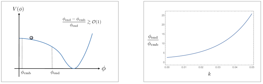
Figure 10: For new inflation, the inflationary expansion occur mostly on the hilltop where $\phi$ is close to the origin. The inflation ends at $\phi_{\text{end}}$ where the potential violates the slow-roll condition and $\phi_{\text{end}}\gg\phi_{\text{cmb}}$.

To find what $c^{\scriptscriptstyle\text{max}}_{\scriptscriptstyle 2n}$ is, we need to first know the field value $\phi_{\text{end}}$ when the inflation ends. This is determined by the number of e-folds $\mathcal{N}^{*}_{e}$ between horizon exit and the end of the inflation, the inflation energy scale $V_{0}$, and the perturbation power spectrum $P_{\zeta}$. In particular, one has

$$\mathcal{N}_{e}= \int H\,dt=\int\frac{H}{\dot{\phi}}\,d\phi=-\int\frac{V}{V^{\prime}}\,d\phi=\int\frac{d\phi}{\sqrt{2\epsilon}}\simeq\frac{\phi_{\text{end}}-\phi_{\text{cmb}}}{\sqrt{2\epsilon}}=\frac{\Delta\phi}{\sqrt{2\epsilon}},$$

$$\Delta\phi\equiv \phi_{\text{end}}-\phi_{\text{cmb}},$$ (A.5)

where we assumed the $\epsilon$ parameter to be nearly constant over the period of inflation. Its value can be determined by the perturbation power spectrum,

$$\epsilon=\frac{1}{24\pi^{2}}\frac{V_{0}}{P_{\zeta}}.$$ (A.6)

For potentials of a new inflation type, we typically have $\Delta\phi\simeq\phi_{\text{end}}$. For example, for the potential

$$V=a-\frac{1}{2}b\,\phi^{2}-c_{n}\phi^{n},$$ (A.7)

for which the relation between $\phi_{\text{end}}$ and $\phi_{\text{cmb}}$ is explicitly computed in Appendix B, the ratio $\phi_{\text{end}}/\phi_{\text{cmb}}$ depends only on the parameter $k\equiv b/a$ and is plotted in the right of Figure 10. We see that the ratio grows for larger $k$, which is not surprising as a larger $k$ requires a smaller $\phi_{\text{cmb}}$ to maintain the same e-folds of inflation. As $\Delta\phi=\phi_{\text{end}}-\phi_{\text{cmb}}$ and $\phi_{\text{end}}\gtrsim\phi_{\text{cmb}}$, we actually have $\Delta\phi\simeq\phi_{\text{end}}$ and hance

$$\phi_{\scriptscriptstyle\text{end}}\simeq\frac{\mathcal{N}^{*}_{e}}{\sqrt{12}\pi}\sqrt{\frac{V_{0}}{P_{\zeta}}}.$$ (A.8)

We define $c^{\epsilon}_{\scriptscriptstyle 2n}$ to be the value of $c_{\scriptscriptstyle 2n}$ such that the $c_{\scriptscriptstyle 2n}\phi^{2n}_{\scriptscriptstyle\text{end}}$ term alone in Eq.(A.2) can violate the $\epsilon$ slow-roll condition, i.e.

$$\frac{1}{2}\left(\frac{2nc^{\epsilon}_{\scriptscriptstyle 2n}\phi^{2n-1}_{\scriptscriptstyle\text{end}}}{V_{0}}\right)^{2}=1,$$ (A.9)

which yields

$$c^{\epsilon}_{\scriptscriptstyle 2n}=\frac{V_{0}}{\sqrt{2}n}\left(\frac{{\mathcal{N}^{*}_{e}}^{2}V_{0}}{12\pi^{2}P_{\zeta}}\right)^{\frac{1-2n}{2}}.$$ (A.10)

Similarly, we define $c^{\eta}_{\scriptscriptstyle 2n}$ such that the $c_{\scriptscriptstyle 2n}\phi^{2n}_{\scriptscriptstyle\text{end}}$ term alone in Eq.(A.3) can violate the $\eta$ slow-roll condition, which yields

$$c^{\eta}_{\scriptscriptstyle 2n}=\frac{V_{0}}{2n(2n-1)}\left(\frac{{\mathcal{N}^{*}_{e}}^{2}V_{0}}{12\pi^{2}P_{\zeta}}\right)^{1-n}.$$ (A.11)

We then define $c^{\scriptscriptstyle\text{max}}_{\scriptscriptstyle 2n}$ to be the minimum of $c^{\epsilon}_{\scriptscriptstyle 2n}$, $c^{\eta}_{\scriptscriptstyle 2n}$ and one,

$$c^{\scriptscriptstyle\text{max}}_{\scriptscriptstyle 2n}=\text{Min}\big{[}c^{\epsilon}_{\scriptscriptstyle 2n},c^{\eta}_{\scriptscriptstyle 2n},1\big{]}.$$ (A.12)

Lastly, we estimate $\phi_{\rm ant}$ originating from scanning over the initial inflaton field value. From the total number of e-folds, we have

$$\mathcal{N}^{tot}_{e}=-\int\frac{V}{V^{\prime}}\,d\phi\simeq\int\frac{V_{0}}{\sum 2n\,c_{2n}\,\phi^{2n-1}}d\phi\simeq\int\frac{V_{0}}{\sum 2n\,c^{\eta}_{2n}\,\phi^{2n-1}}\,d\phi\simeq\int\frac{V_{0}}{2n\,c^{\eta}_{2n}\,\phi^{2n-1}}\,d\phi$$ (A.13)

where in the third equality we used $c^{\eta}_{2n}$ to replace $c_{n}$ because when the potential terms are relevant to the inflationary dynamics, their coefficients will be bounded by $c^{max}_{2n}$ and $c^{\eta}_{2n}<c^{\epsilon}_{2n}$ when the energy scale $V_{0}$ is small. In the last equality, we approximated the summation by the $n\mathchar 45\relax$th term because all the relevant potential terms are comparable. After performing the integral from $\phi_{i}$ to $\phi_{end}$, because the integral is dominated by the $\phi_{i}$ term, we obtain

$$\mathcal{N}^{tot}_{e}\simeq\frac{2n-1}{2(n-1)}\left(\frac{12\pi^{2}P_{\zeta}}{{\mathcal{N}^{*}_{e}}^{2}V_{0}}\right)^{1-n}\phi_{i}^{2(1-n)},$$ (A.14)

which gives

$$\phi_{\rm ant}\propto\sqrt{\frac{V_{0}}{P_{\zeta}}}.$$ (A.15)

The probability $P\propto V_{0}\phi_{\rm ant}\prod_{n=1}^{\infty}c^{\scriptscriptstyle\text{max}}_{\scriptscriptstyle 2n}$ is a function of $V_{0}$ and $P_{\zeta}$. We plot the unnormalized probability function in the left panel of Figure 11 for three different $P_{\zeta}$’s. One can see that the probability is strongly biased toward large perturbation. In addition, there are several kinks along each curves. To understand these kinks more, it is illustrative to plot the first few $c^{\scriptscriptstyle\text{max}}_{\scriptscriptstyle 2n}$’s. In the right panel of Figure 11, we see that the coefficients for higher dimensional operators, those with $n\geq 3$, have $c^{\scriptscriptstyle\text{max}}_{\scriptscriptstyle 2n}=1$ for small $V_{0}$. This is because $\phi_{\scriptscriptstyle\text{end}}\propto\sqrt{V_{0}}$ as shown in Eq.(A.8) and hence for small $V_{0}$, the higher-dimensional operators are Planck-suppressed and irrelevant to inflationary dynamics. This is also the reason why assuming $c^{\scriptscriptstyle\text{max}}_{\scriptscriptstyle 2n}$’s are independent on each other does not change the qualitative result. Only the lower dimensional coefficients can affect the higher ones but not vice versa. As we increase the inflation energy scale, the field displacement becomes larger and hence higher-dimensional operators become relevant and their required coefficients start to decrease from one. This translates to the kinks shown in the left panel of Figure 11. For instance, in Figure 11 we see that, for $P_{\zeta}=10^{-9}$, $V_{0}\sim 10^{-17}$ indicated by the orange dashed line is precisely the scale where the octet term starts to be relevant and require fine-tuning. Also note that, regardless of the value of $P_{\zeta}$, the amount of fine-tuning is minimal when the octet operator just became relevant.

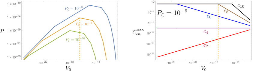
Figure 11: Left: The probability $\mathcal{P}$ for different primordial perturbation amplitude $P_{\zeta}$. Right: The values of $c^{\scriptscriptstyle\text{max}}_{\scriptscriptstyle 2},c^{\scriptscriptstyle\text{max}}_{\scriptscriptstyle 4},c^{\scriptscriptstyle\text{max}}_{\scriptscriptstyle 6},c^{\scriptscriptstyle\text{max}}_{\scriptscriptstyle 8}$ and $c^{\scriptscriptstyle\text{max}}_{\scriptscriptstyle 10}$ as a function of $V_{0}$ with $P_{\zeta}=10^{-9}$. Notice that $c^{\scriptscriptstyle\text{max}}_{\scriptscriptstyle 8}$ starts to decrease from 1 at $V_{0}\sim 10^{-16}$, where $\mathcal{P}$ reaches maximum.

We compute the probability to obtain a cosmic perturbation $P_{\zeta}$. As we have observed, the probability $P$ peaks at the point when the octet becomes relevant, i.e. when $c^{\eta}_{8}=1$. This gives us the energy scale $V^{max}_{0}$ where the fine-tuning is minimal,

$$V^{max}_{0}=\frac{1}{2\sqrt{14}}\left(\frac{{\mathcal{N}^{*}_{e}}^{2}}{12\pi^{2}P_{\zeta}}\right)^{-\frac{3}{2}}.$$ (A.16)

When we integrate out $V_{0}$ the integration is dominated by the region around $V^{max}_{0}$, we therefore have

$$P\propto V^{max}_{0}\phi_{\rm ant}c^{max}_{2}c^{max}_{4}c^{max}_{6}\propto P_{\zeta}^{\frac{19}{4}}.$$ (A.17)

This can be understood as $P_{\zeta}$ obeying the distribution

$$P(P_{\zeta})dP_{\zeta}\propto P_{\zeta}^{\frac{15}{4}}dP_{\zeta}.$$ (A.18)

The probability is strongly biased toward large $P_{\zeta}$. Unless there exists a strong anthropic bound disfavoring $P_{\zeta}$ larger than the observed one, it is unlikely that general new inflation with $Z_{2}$ symmetry results in our observed universe. Our analysis is also applicable to the case with $U(1)$ symmetry because the radial direction is essentially $Z_{2}$ symmetric, while the angular direction is flat and does not affect the inflationary dynamics at the background level.

For completeness, we continue our further analysis of general new inflation with $Z_{2}$ symmetry in the next section. In particular, assuming that the perturbation amplitude $P_{\zeta}$ is fixed to the observed value for some reason, we investigate the probability distribution of spectral index $n_{s}$. We will find that it is probabilistically favored to have a spectral index $n_{s}\simeq 0.96$, which is quite remarkable.

Appendix B New Inflation and the Most Probable Spectral Index

In Appendix A we found that when considering inflation with $Z_{2}$ symmetry, we need to fine-tune terms at least up to the octet order,

$$V=V_{0}+c_{\scriptscriptstyle 2}\phi^{2}+c_{\scriptscriptstyle 4}\phi^{4}+c_{\scriptscriptstyle 6}\phi^{6}+c_{\scriptscriptstyle 8}\phi^{8}.$$ (B.1)

Nevertheless, for simplicity we will consider potential of the form

$$V=a-\frac{1}{2}b\,\phi^{2}-c_{n}\phi^{n}-c_{m}\phi^{m}$$ (B.2)

where the $c_{n}$ term dominates over the $c_{m}$ term and the latter is treated perturbatively. Namely, we consider the case where $c_{m}$ is sufficiently small and $c_{m}\phi^{m}<c_{n}\phi^{n}$. We can then extract the physics of the complete octet model, Eq.(B.1), by extrapolation. In Eq.(B.2) we make quadratic term explicitly negative as we now consider cases where the inflaton rolls down from $\phi=0$.

The number of e-folds $\mathcal{N}_{e}$ which the inflation would last before it ends and the corresponding field value $\phi_{\scriptscriptstyle\mathcal{N}_{e}}$ has the relation

$$\mathcal{N}_{e} =\int^{\phi_{\scriptscriptstyle\mathcal{N}_{e}}}_{\phi_{end}}\frac{V}{\partial V/\partial\phi}\,d\phi$$

$$\simeq\int^{\phi_{\scriptscriptstyle\mathcal{N}_{e}}}_{\phi_{end}}\frac{a}{-b\phi-nc_{n}\phi^{n-1}-mc_{m}\phi^{m-1}}\,d\phi$$

$$\simeq a\int^{\phi_{\scriptscriptstyle\mathcal{N}_{e}}}_{\phi_{end}}\left[\frac{1}{b\phi+nc_{n}\phi^{n-1}}-\frac{m\phi^{m-1}}{b\phi+nc_{n}\phi^{n-1}}\,c_{m}\right]d\phi$$

$$=\frac{1}{(n-2)k}\ln\left(\frac{k\phi_{\scriptscriptstyle\mathcal{N}_{e}}^{2-n}+\frac{c_{n}}{a}n}{k\phi^{2-n}_{end}+\frac{c_{n}}{a}n}\right)-\frac{1}{k}\left[\mathcal{F}(\phi_{end})-\mathcal{F}({\phi_{\scriptscriptstyle\mathcal{N}_{e}}})\right]c_{m}$$ (B.3)

where we defined $k\equiv b/a$ and

$$\mathcal{F}(\phi)\equiv\frac{m}{n-2}\frac{\phi^{m-2}}{ak}\left\{\left(\frac{n-m}{m-2}\right){}_{2}F_{1}\left(1,\frac{m-2}{n-2};\frac{n+m-4}{n-2};-\frac{nc_{n}}{ak}\phi^{n-2}\right)+\frac{ak}{ak+nc_{n}\phi^{n-2}}\right\}.$$ (B.4)

Here ${{}_{2}F_{1}}$ is the hypergeometric function and $\phi_{end}$ is the field value where the inflation ends, determined by the slow-roll condition. In particular, the inflation ends when the $\eta$-parameter reaches -1, which yields

$$\phi^{n-2}_{end}\simeq\frac{a}{n(n-1)c_{n}}.$$ (B.5)

Solving Eq.(B.3) for $\phi_{\scriptscriptstyle\mathcal{N}_{e}}(\mathcal{N}_{e})$ perturbatively in $c_{m}$, that is, with $\phi_{\scriptscriptstyle\mathcal{N}_{e}}(\mathcal{N}_{e})=\phi_{\scriptscriptstyle\mathcal{N}_{e}}^{(0)}+c_{m}\,\phi_{\scriptscriptstyle\mathcal{N}_{e}}^{(1)}$, one has

$$\phi_{\scriptscriptstyle\mathcal{N}_{e}}^{(0)}=\left[\frac{a}{c_{n}}kf_{n}(k)\right]^{\frac{1}{n-2}},\quad\text{ and }\quad\phi_{\scriptscriptstyle\mathcal{N}_{e}}^{(1)}=\phi_{0}\,c_{n}^{-\frac{m-2}{n-2}}a^{\frac{m-n}{n-2}}g_{n,m}(k)$$ (B.6)

where

$$f_{n}(k)\equiv\frac{1}{n}\frac{1}{\left(\left[1+(n-1)k\right]e^{(n-2)k\mathcal{N}_{e}}-1\right)}$$ (B.7)

and

$$g_{n,m}(k)\equiv \,\frac{m(n-m)}{(n-2)(m-2)}\left(1+nf_{n}\right)\times$$

$$\hskip 28.45274pt\Bigg{\{}k^{\frac{m-n}{n-2}}f_{n}^{\frac{m-2}{n-2}}\left[{}_{2}F_{1}\left(1,\frac{m-2}{n-2};\frac{n+m-4}{n-2},-nf_{n}\right)+\frac{1}{1+nf_{n}}\right]$$

$$\hskip 56.9055pt\left.-\left(\frac{1}{n(n-1)}\right)^{\frac{m-2}{n-2}}\frac{1}{k}\left[{}_{2}F_{1}\left(1,\frac{m-2}{n-2};\frac{n+m-4}{n-2},-\frac{1}{(n-1)k}\right)+\frac{1}{1+\frac{1}{(n-1)k}}\right]\right\}.$$ (B.8)

The spectral index $n_{s}$ and perturbation power spectrum $P_{\zeta}$ when inflation can last another $\mathcal{N}_{e}$ of e-folds before it ends is then given by

$$n_{s} =1+2\eta-6\epsilon$$

$$=1-2k-2n(n-1)kf_{n}-3a^{\frac{2}{n-2}}c_{n}^{-\frac{2}{n-2}}k^{\frac{2n-2}{n-2}}\left(1+nf_{n}\right)^{2}f_{n}^{\frac{2}{n-2}}$$

$$\hskip 28.45274pt+\Bigg{\{}2a^{\frac{m-n}{n-2}}c_{n}^{-\frac{m-2}{n-2}}\left[m(1-m)k^{\frac{m-2}{n-2}}f_{n}^{\frac{m-2}{n-2}}-n(n-1)(n-2)k\,f_{n}\,g_{n,m}\right]$$

$$\hskip 42.67912pt-6a^{\frac{m-n+2}{n-2}}c_{n}^{-\frac{m}{n-2}}k^{\frac{n}{n-2}}f_{n}^{\frac{2}{n-2}}(1+nf_{n})\left(mk^{\frac{m-2}{n-2}}f_{n}^{\frac{m-2}{n-2}}+k\,g_{n,m}+n(n-1)k\,f_{n}\,g_{n,m}\right)\Bigg{\}}c_{m},$$ (B.9)

$$P_{\zeta} =\frac{1}{24\pi^{2}}\frac{V}{\epsilon}$$

$$=\frac{a^{\frac{n-4}{n-2}}k^{\frac{-2n+2}{n-2}}f_{n}^{-\frac{2}{n-2}}}{12\pi^{2}\left(1+nf_{n}\right)^{2}}\left[c^{\frac{2}{n-2}}_{n}-c^{\frac{4-m}{n-2}}_{n}\,c_{m}\,\frac{2a^{\frac{m-n}{n-2}}\left(mk^{\frac{m-n}{n-2}}f^{\frac{m-2}{n-2}}_{n}+g_{n,m}+n(n-1)\,f_{n}\,g_{n,m}\right)}{(1+nf_{n})}\right].$$ (B.10)

By taking the inverse of Eq.(B.10) perturbatively in $c_{m}$, one obtain $c_{n}=c_{n}^{(0)}+c_{m}\,c_{n}^{(1)}$ with

$$c^{(0)}_{n}=(12\pi^{2})^{\frac{n-2}{2}}a^{\frac{4-n}{2}}k^{n-1}f_{n}\left(1+nf_{n}\right)^{n-2}P_{\zeta}^{\frac{n-2}{2}},$$ (B.11)

and

$$c^{(1)}_{n}=\frac{n-2}{2}{c^{(0)}_{n}}^{\frac{n-m+2}{n-2}}\frac{2a^{\frac{m-n}{n-2}}\left(mk^{\frac{m-n}{n-2}}f_{n}^{\frac{m-2}{n-2}}+g_{n,m}+n(n-1)f_{n}\,g_{n,m}\right)}{1+nf_{n}}.$$ (B.12)

With Eq.(B.9), (B.11) and (B.12), the relation between the spectral index $n_{s}$ and the parameter $k$ is plotted in Figure 12 for various set of $(n,m)$. We set the parameter $a=10^{-16}$, the number of e-folds $\mathcal{N}_{e}=55$, and the perturbation power spectrum to the observed value, $P_{\zeta}=2.2\times 10^{-9}$. The parameter $c_{m}$ is bounded by the requirement that the perturbation holds, i.e. $c_{m}\phi^{m}<c_{n}\phi^{n}$. As $\phi_{end}>\phi_{\scriptscriptstyle\mathcal{N}_{e}}$, the bound of $c_{m}$ is therefore

$$|c_{m}|<\begin{cases}c_{n}\phi_{\scriptscriptstyle\mathcal{N}_{e}}^{n-m}&\quad(n>m),\\ \\ c_{n}\phi_{end}^{n-m}&\quad(n<m).\end{cases}$$ (B.13)

We first look at the case with quartic and sextic terms, shown on the left of Figure 12. Note that the quartic-dominant case is excluded by observation. One generic feature that appears for all $(n,m)$ is that when $n<m$, a positive perturbation ($c_{m}>0$) leads to a spectral index closer to scale-invariance, i.e. $n_{s}=1$, while a negative perturbation ($c_{m}<0$) makes $n_{s}$ deviate away from $1$. This might be counterintuitive as the potential

$$V=a-\frac{1}{2}b\phi^{2}-c_{n}\phi^{n}-c_{m}\phi^{m},$$ (B.14)

is flatter when $c_{m}<0$ and we would have expected a spectral index closer to $1$. However, a flatter potential also means the inflaton moves slower before it reaches $\phi_{end}$, and hence the field value can be closer to $\phi_{end}$ (but farther away from zero) while giving the same number of e-foldings as shown in the left of Figure 13. As the field is farther away from zero where the potential is the flattest, the spectral index can deviate from -1. The two effects, flatter potential and larger $\phi_{\scriptscriptstyle\mathcal{N}_{e}}$, compete with each other and the latter wins when $n<m$. On the other hand, for $n>m$ the effect of flatter potential dominates and a negative perturbation ($c_{m}<0$) leads to spectral index closer to 1. The fact that the two cases, $n>m$ and $n<m$, behave oppositely and the region of positive perturbation lies between two unperturbed curves makes us confident that one can extrapolate our perturbative treatment to the case where the $c_{n}$ term and $c_{m}$ term comparable – it simply lies between the two perturbative regions where one dominates the other, as shown in the right in Figure 13.

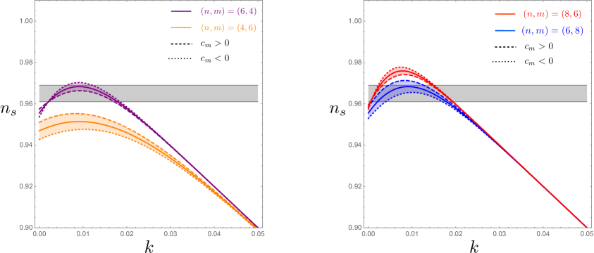
Figure 12: The $n_{s}-k$ plot for different set of $(n,m)$. The dashed lines corresponds to the boundary of positive perturbation, $c_{m}>0$, while the dotted ones represents negative perturbation, $c_{m}<0$. The grey region shows the current observational value.

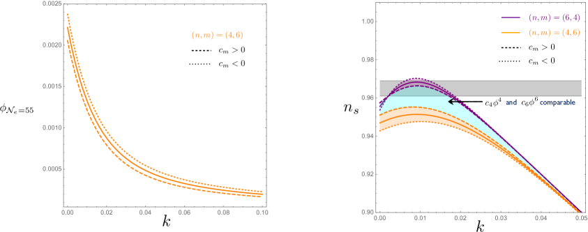
Figure 13: (Left) The $\phi-k$ plot for $(n,m)=(4,6)$. One can see that for the same $k$, $\phi$ is larger when $c_{m}<0$. (Right) Even though our treatment is perturbative, the case where $c_{n}\phi^{n}$ and $c_{m}\phi^{m}$ are comparable should continuously connect the two perturbative regions.

In Figure 12 we see that sextic dominant models, $n=6$, with either quartic perturbation ($m=4$) or octet perturbation ($m=8$), fit the observation quite well when $k\lesssim 0.018$. We discuss the chance for $k$ to lie in this region. We will focus on the following analysis without perturbation,

$$V=a-\frac{1}{2}b\,\phi^{2}-c_{n}\phi^{n}$$ (B.15)

as additional perturbation $c_{m}\phi^{m}$ does not change the end result significantly. We assume the parameter in the Lagrangian $a$, $b$ and $c_{n}$ has uniform probability distribution and also take the probabilistic nature of the initial condition into account. Using the definition $b=ak$, Eq.(B.6) and Eq.(B.11), one has

$$\int^{\phi_{\rm ant}}_{0}d\phi_{i}\int da\,db\,dc_{n}=\int da\,dP_{\zeta}\,dk\,(12\pi^{2})^{\scriptscriptstyle\frac{n-3}{2}}a^{\scriptscriptstyle\frac{7-n}{2}}P_{\zeta}^{\scriptscriptstyle\frac{n-5}{2}}k^{n-2}f_{n}\left(1+n\,f_{n}\right)^{n-3},$$ (B.16)

where we need to integrate over $a$ to obtain the probability distribution of $k$ for a given $P_{\zeta}$. For $n=6$ and 8, the integration over $a$ is divergent with an upper bound $a_{max}$ that is around $10^{-17}$ where only terms below the octec order require fine-tuning. The exact upper bound $a_{max}$ is correlated with the upper bound for $c_{n}$, but most importantly $a_{max}$ is independent on $k$ and hence the integration over $a$ does not give an additional $k$-dependence. In sum, for the cases of interest, the probability distribution of $k$ is

$$\mathcal{P}_{k}\,dk=k^{n-2}f_{n}\left(1+n\,f_{n}\right)^{n-3}\,dk,$$ (B.17)

where $f_{n}(k)$ is defined in Eq.(B.7), and the plot for $n=6$ is given in Figure 14. The shaded area corresponds to the interval $\mathcal{I}$ of $k$ that yields spectral index $n_{s}>0.96$. The probability for $k$ to lie in this region for $n=6$ is

$$P_{n_{s}>0.96}=\frac{\int_{\mathcal{I}}\mathcal{P}_{k}\,dk}{\int^{\infty}_{0}\mathcal{P}_{k}\,dk}\simeq 0.49.$$ (B.18)

and the distribution $\mathcal{P}_{k}$ peaks at $k\simeq 0.016$, which yields a spectral index of $n_{s}=0.963$. Overall it is quite remarkable that once one matches the observed perturbation power spectrum $P_{\zeta}$, there is about a few ten chance to achieve the observed spectral index without much further fine-tuning in general new inflation with $Z_{2}$ symmetry. But as we discussed in Sec.A, the observed $P_{\zeta}$ can be obtained without significant fine-tuning only if there is a strong anthropic bound on $P_{\zeta}$ right at the observed value which seems to be unlikely.

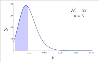
Figure 14: The normalized probability distribution of $k$ for $n=6$. The shaded area corresponds to the interval of $k$ that yields spectral index $n_{s}>0.96$.

References

- [1] A. H. Guth, “The Inflationary Universe: A Possible Solution to the Horizon and Flatness Problems,” Phys. Rev. D23 (1981) 347–356.
- [2] D. Kazanas, “Dynamics of the Universe and Spontaneous Symmetry Breaking,” Astrophys. J. 241 (1980) L59–L63.
- [3] V. F. Mukhanov and G. V. Chibisov, “Quantum Fluctuations and a Nonsingular Universe,” JETP Lett. 33 (1981) 532–535. [Pisma Zh. Eksp. Teor. Fiz.33,549(1981)].
- [4] S. W. Hawking, “The Development of Irregularities in a Single Bubble Inflationary Universe,” Phys. Lett. 115B (1982) 295.
- [5] A. A. Starobinsky, “Dynamics of Phase Transition in the New Inflationary Universe Scenario and Generation of Perturbations,” Phys. Lett. 117B (1982) 175–178.
- [6] A. H. Guth and S. Y. Pi, “Fluctuations in the New Inflationary Universe,” Phys. Rev. Lett. 49 (1982) 1110–1113.
- [7] J. M. Bardeen, P. J. Steinhardt, and M. S. Turner, “Spontaneous Creation of Almost Scale - Free Density Perturbations in an Inflationary Universe,” Phys. Rev. D28 (1983) 679.
- [8] A. D. Linde, “A New Inflationary Universe Scenario: A Possible Solution of the Horizon, Flatness, Homogeneity, Isotropy and Primordial Monopole Problems,” Phys. Lett. 108B (1982) 389–393.
- [9] A. Albrecht and P. J. Steinhardt, “Cosmology for Grand Unified Theories with Radiatively Induced Symmetry Breaking,” Phys. Rev. Lett. 48 (1982) 1220–1223.
- [10] A. A. Starobinsky, “A New Type of Isotropic Cosmological Models Without Singularity,” Phys. Lett. B91 (1980) 99–102.
- [11] L. Susskind, “The Anthropic landscape of string theory,” arXiv:hep-th/0302219 [hep-th].
- [12] R. Bousso and J. Polchinski, “Quantization of four form fluxes and dynamical neutralization of the cosmological constant,” JHEP 06 (2000) 006, arXiv:hep-th/0004134 [hep-th].
- [13] A. Vilenkin, “Predictions from quantum cosmology,” Phys. Rev. Lett. 74 (1995) 846–849, arXiv:gr-qc/9406010 [gr-qc].
- [14] S. Weinberg, “Anthropic Bound on the Cosmological Constant,” Phys. Rev. Lett. 59 (1987) 2607.
- [15] B. Freivogel, M. Kleban, M. Rodriguez Martinez, and L. Susskind, “Observational consequences of a landscape,” JHEP 03 (2006) 039, arXiv:hep-th/0505232 [hep-th].
- [16] A. H. Guth, D. I. Kaiser, and Y. Nomura, “Inflationary paradigm after Planck 2013,” Phys. Lett. B733 (2014) 112–119, arXiv:1312.7619 [astro-ph.CO].
- [17] S. R. Coleman and F. De Luccia, “Gravitational Effects on and of Vacuum Decay,” Phys. Rev. D21 (1980) 3305.
- [18] J. R. Gott, “Creation of Open Universes from de Sitter Space,” Nature 295 (1982) 304–307.
- [19] A. D. Linde and A. Mezhlumian, “Inflation with ,” Phys. Rev. D52 (1995) 6789–6804, arXiv:astro-ph/9506017 [astro-ph].
- [20] A. Vilenkin and S. Winitzki, “Probability distribution for omega in open universe inflation,” Phys. Rev. D55 (1997) 548–559, arXiv:astro-ph/9605191 [astro-ph].
- [21] Planck Collaboration, N. Aghanim et al., “Planck 2018 results. VI. Cosmological parameters,” arXiv:1807.06209 [astro-ph.CO].
- [22] H. Martel, P. R. Shapiro, and S. Weinberg, “Likely values of the cosmological constant,” Astrophys. J. 492 (1998) 29, arXiv:astro-ph/9701099 [astro-ph].
- [23] J. D. Barrow and P. Saich, “Growth of large-scale structure with a cosmological constant,” Monthly Notices of the Royal Astronomical Society 262 (June, 1993) 717–725.
- [24] J. D. Barrow and F. J. Tipler, The Anthropic Cosmological Principle. Oxford U. Pr., Oxford, 1986.
- [25] R. Bousso and R. Harnik, “The Entropic Landscape,” Phys. Rev. D82 (2010) 123523, arXiv:1001.1155 [hep-th].
- [26] M. Tegmark and M. J. Rees, “Why is the Cosmic Microwave Background fluctuation level 10**(-5)?,” Astrophys. J. 499 (1998) 526–532, arXiv:astro-ph/9709058 [astro-ph].
- [27] M. Tegmark, A. Aguirre, M. Rees, and F. Wilczek, “Dimensionless constants, cosmology and other dark matters,” Phys. Rev. D73 (2006) 023505, arXiv:astro-ph/0511774 [astro-ph].
- [28] A. D. Linde, D. A. Linde, and A. Mezhlumian, “From the Big Bang theory to the theory of a stationary universe,” Phys. Rev. D49 (1994) 1783–1826, arXiv:gr-qc/9306035 [gr-qc].
- [29] R. Bousso, “Holographic probabilities in eternal inflation,” Phys. Rev. Lett. 97 (2006) 191302, arXiv:hep-th/0605263 [hep-th].
- [30] A. De Simone, A. H. Guth, M. P. Salem, and A. Vilenkin, “Predicting the cosmological constant with the scale-factor cutoff measure,” Phys. Rev. D78 (2008) 063520, arXiv:0805.2173 [hep-th].
- [31] R. Bousso, B. Freivogel, and I.-S. Yang, “Properties of the scale factor measure,” Phys. Rev. D79 (2009) 063513, arXiv:0808.3770 [hep-th].
- [32] Y. Nomura, “Physical Theories, Eternal Inflation, and Quantum Universe,” JHEP 11 (2011) 063, arXiv:1104.2324 [hep-th].
- [33] J. Garriga and A. Vilenkin, “Watchers of the multiverse,” JCAP 1305 (2013) 037, arXiv:1210.7540 [hep-th].
- [34] B. A. Ovrut and P. J. Steinhardt, “Supersymmetry and Inflation: A New Approach,” Phys. Lett. 133B (1983) 161–168.
- [35] R. Holman, P. Ramond, and G. G. Ross, “Supersymmetric Inflationary Cosmology,” Phys. Lett. 137B (1984) 343–347.
- [36] A. B. Goncharov and A. D. Linde, “Chaotic Inflation in Supergravity,” Phys. Lett. 139B (1984) 27–30.
- [37] G. D. Coughlan, R. Holman, P. Ramond, and G. G. Ross, “Supersymmetry and the Entropy Crisis,” Phys. Lett. 140B (1984) 44–48.
- [38] E. J. Copeland, A. R. Liddle, D. H. Lyth, E. D. Stewart, and D. Wands, “False vacuum inflation with Einstein gravity,” Phys. Rev. D49 (1994) 6410–6433, arXiv:astro-ph/9401011 [astro-ph].
- [39] M. Tegmark, “What does inflation really predict?,” JCAP 0504 (2005) 001, arXiv:astro-ph/0410281 [astro-ph].
- [40] A. Masoumi, A. Vilenkin, and M. Yamada, “Inflation in random Gaussian landscapes,” JCAP 1705 no. 05, (2017) 053, arXiv:1612.03960 [hep-th].
- [41] J. D. Barrow, “The Isotropy of the Universe,” Quarterly Journal of the Royal Astronomical Society 23 (Sept., 1982) 344.
- [42] K. Kumekawa, T. Moroi, and T. Yanagida, “Flat potential for inflaton with a discrete R invariance in supergravity,” Prog. Theor. Phys. 92 (1994) 437–448, arXiv:hep-ph/9405337 [hep-ph].
- [43] K. I. Izawa and T. Yanagida, “Natural new inflation in broken supergravity,” Phys. Lett. B393 (1997) 331–336, arXiv:hep-ph/9608359 [hep-ph].
- [44] K. Harigaya, M. Ibe, and T. T. Yanagida, “Lower Bound on the Garvitino Mass TeV in -Symmetry Breaking New Inflation,” Phys. Rev. D89 no. 5, (2014) 055014, arXiv:1311.1898 [hep-ph].
- [45] V. Agrawal, S. M. Barr, J. F. Donoghue, and D. Seckel, “The Anthropic principle and the mass scale of the standard model,” Phys. Rev. D57 (1998) 5480–5492, arXiv:hep-ph/9707380 [hep-ph].
- [46] L. J. Hall, D. Pinner, and J. T. Ruderman, “The Weak Scale from BBN,” JHEP 12 (2014) 134, arXiv:1409.0551 [hep-ph].