MI-TH-187

We study extremal static dyonic black holes in four-dimensional Einstein-Maxwell-Dilaton theory, for general values of the constant $a$ in the exponential coupling $e^{a\phi}$ of the dilaton to the Maxwell kinetic term. Explicit solutions are known only for $a=0$, $a=1$ and $a=\sqrt{3}$, and for general $a$ when the electric and magnetic charges $Q$ and $P$ are equal. We obtain solutions as power series expansions around $Q=P$, in terms of a small parameter $\epsilon=a^{-1}\,\log(Q/P)$. Using these, and also solutions constructed numerically, we test a relation between the mass and the charges that had been conjectured long ago by Rasheed. We find that although the conjecture is not exactly correct it is in fact quite accurate for a wide range of the black hole parameters. We investigate some improved conjectures for the mass relation. We also study the circumstances under which entropy super-additivity, which is related to Hawking’s area theorem, is violated. This extends beyond previous examples exhibited in the literature for the particular case of $a=\sqrt{3}$ dyonic black holes.

$\,{}^{\dagger}$gengwj@mail.bnu.edu.cn   $\,{}^{\ddagger}$bkg218@lehigh.edu  $\,{}^{*}$mrhonglu@gmail.com  $\,{}^{\sharp}$pope@physics.tamu.edu

1 Introduction

The Einstein-Maxwell-Dilaton (EMD) theory in four dimensions, and its black hole solutions, have been investigated extensively in the last few decades. The theory is a generalization of Einstein-Maxwell theory in which a real dilatonic scalar field $\phi$ is included, coupling not only to gravity but also, via a non-minimal term, to the Maxwell field. The Lagrangian is given by

$${\cal L}=\sqrt{-g}\Big{(}R-{\textstyle{\frac{\scriptstyle 1}{\scriptstyle 2}}}(\partial\phi)^{2}-{\textstyle{\frac{\scriptstyle 1}{\scriptstyle 4}}}e^{a\phi}F^{2}\Big{)}\,,\qquad F=dA\,.$$ (1.1)

For certain specific values of the dilaton coupling constant $a$, the EMD theory corresponds to particular truncations of four-dimensional maximal ${\cal N}=8$ supergravity, and for this reason much attention has been focused on these cases because of their relevance in string theory. In fact, these special cases all fall within the consistent truncation of the ${\cal N}=8$ theory to ${\cal N}=2$ STU supergravity [1], which comprises pure ${\cal N}=2$ supergravity coupled to three vector multiplets. The further truncations to special cases of the EMD theory arise by setting some of the STU supergravity fields, or combinations of fields, to zero. The various truncations lead to an EMD theory with $a$ taking one of the values $a=0$, ${\textstyle{\frac{\scriptstyle 1}{\scriptstyle\sqrt{3}}}}$, 1 or $\sqrt{3}$ [2, 3, 4]. The case of $a=0$ can also be reduced to pure Einstein-Maxwell theory, since the dilaton can be consistently truncated in this case. When $a=\sqrt{3}$ the EMD theory also corresponds to the Kaluza-Klein reduction of five-dimensional pure gravity. Because of the enhanced Cremer-Julia like symmetries [5, 6, 7, 8] of the dimensional reduction of the supergravity theories, in these four special cases among the general EMD theories, one can use solution-generating techniques to construct charged black hole solutions from neutral ones.

Static non-extremal black holes in the general four-dimensional EMD theory were constructed in [9, 10]. Explicit solutions are obtainable for all values of the dilaton coupling in the case where the black hole carries purely electric or purely magnetic charge. Dyonic black holes, carrying both electric and magnetic charge, can be constructed explicitly in the three cases $a=0$, $a=1$ and $a=\sqrt{3}$. When $a=0$ this is rather trivial, since there then exists a duality symmetry of the equations of motion, allowing a purely electric or purely magnetic Reissner-Nordström (RN) black hole to be transformed into a dyonic one. Rotating black holes have also been studied in the EMD theory. In particular, the dyonic rotating solutions in the $a=\sqrt{3}$ EMD theory were constructed by Rasheed in [11] (see also [12]).

In this paper we shall focus our attention on static black hole solutions in the EMD theories; in particular on the dyonically-charged black holes. As mentioned above, these can be constructed explicitly when $a=0$, 1 or $\sqrt{3}$, but no explicit solutions are known for other values of the dilaton coupling, except when the electric and magnetic charges are equal, in which case the dilaton is constant and the solution reduces to a dyonic Reissner-Nordström black hole. We shall therefore use various approximation and numerical techniques in order to investigate the nature of the dyonic black hole solutions for general values of $a$. We shall, furthermore, restrict our attention to the case of extremal dyonic black holes.

In the extremal limit, the mass of a black hole is no longer specifiable independently, but rather, it is a definite function of the electric and magnetic charges. For the three special cases mentioned above, where explicit solutions are known, the mass $M$ is given in terms of the electric charge $Q$ and magnetic charge $P$ by the relations

$$a=0\,, \quad M=2\sqrt{Q^{2}+P^{2}}\,,$$ (1.2)

$$a=1\,, \quad M=\sqrt{2}(Q+P)\,,$$ (1.3)

$$a=\sqrt{3}\,, \quad M=(Q^{\frac{2}{3}}+P^{\frac{2}{3}})^{\frac{3}{2}}\,.$$ (1.4)

Based on these expressions, and also the known mass-charge relations of extremal single-charge or equal-charge solutions, Rasheed [11] conjectured a possible formula for the mass as a function of $Q$ and $P$ for dyonic extremal black holes for general values of the dilaton coupling constant $a$, namely

$$M={\frac{2}{\sqrt{a^{2}+1}}}(Q^{b}+P^{b})^{{\frac{1}{b}}}\,,\qquad b={\frac{2\log 2}{\log(2a^{2}+2)}}\,.$$ (1.5)

The approximate solutions that we are able to construct for general values of the dilaton coupling allow us to test the validity of this conjecture, and in fact, we are able to establish that it does not hold. However, we are able to obtain an approximate relation, valid in the regime when $Q$ and $P$ are close to one another, but we have not found a simple closed-form relation for $M=M(Q,P)$ that is valid for general values of the dilaton coupling $a$.

The other purpose of this paper is to study a thermodynamic property of black holes known as entropy super-additivity or sub-additivity. Gravitating systems, and black holes especially, have thermodynamic properties that are rather different from those of more conventional laboratory systems. This is related to the the long-range nature of the gravitational field, and the fact that it cannot be screened. In particular, the entropy does not scale homogeneously with the mass of the black hole. Unlike in more conventional thermodynamic systems, the entropy of a black hole is not a concave function of the other extensive variables. A property that does hold, however, in many black hole solutions, is that the entropy is a super-additive function. That is, if one considers black hole solutions with mass $M$, angular momentum $J$, charges $Q^{i}$, and entropy $S=S(M,J,Q^{i})$, then for two such sets of parameters $(M_{1},J_{1},Q^{i}_{1})$ and $(M_{2},J_{2},Q^{i}_{2})$, entropy super-additivity asserts that

$$S(M_{1}+M_{2},J_{1}+J_{2},Q^{i}_{1}+Q^{i}_{2})\geq S(M_{1},J_{1},Q^{i}_{1})+S(M_{2},J_{2},Q^{i}_{2})\,,$$ (1.6)

(with all angular momenta and charges taken, without loss of generality, to be non-negative). This property was observed for Kerr-Newman black holes in [13], and was recently explored for a variety of black holes in [14]. Situations where entropy super-additivity is not satisfied seem to be rather rare, and just one example was exhibited in [14], namely the dyonic black hole in $a=\sqrt{3}$ EMD theory. Since entropy super-additivity holds for the other explicitly known examples of dyonic EMD black holes (i.e. for $a=0$ and $a=1$), it is therefore of considerable interest to investigate this question for the case of general dilaton coupling $a$.

The paper is organized as follows: In section 2 we obtain the equations of motion for the various functions in the ansatz for static dyonic solutions, including the equation relating the metric functions in the case of extremal solutions. In section 3 we discuss the known explicit static solutions, including purely electric and purely magnetic black holes for all values of the dilaton coupling $a$, and the dyonic black hole solutions for the special cases $a=0$, $a=1$ and $a=\sqrt{3}$. In section 4 we present our construction of extremal dyonic solutions for general dilaton coupling $a$, as power series expansions in the parameter $\epsilon=a^{-1}\,\log(Q/P)$, by perturbing around the exactly-solvable case where $Q=P$. We then use these solutions to investigate candidate formulae giving the mass in terms of the electric and magnetic charges of the extremal black holes. We also test the mass formulae in the regime far away from $Q\sim P$, by constructing numerical solutions for the dyonic black holes. In section 5 we examine the conditions under which entropy super-additivity holds, showing that counter-examples can arise when $a$ is sufficiently large. Finally, after conclusions in section 6, we give some further details of our series expansion results in appendix A, and our numerical procedures in appendix B.

2 The theory and equations of motion

In this section, we study the EMD theory (1.1), focusing on constructing spherically symmetric black hole solutions. It is sometimes convenient to express the dilaton coupling constant $a$ as [4]

$$a^{2}={\frac{4}{N}}-1\,.$$ (2.1)

When $N=1$, 2, 3 or 4, corresponding to $a=\sqrt{3}$, 1, ${\textstyle{\frac{\scriptstyle 1}{\scriptstyle\sqrt{3}}}}$ or 0, the theory can be consistently embedded in a supergravity theory, with $N$ denoting the number of basic stringy building blocks in string or M-theory [4]. The equations of motion are

$$\Box\phi = {\textstyle{\frac{\scriptstyle 1}{\scriptstyle 4}}}ae^{a\phi}F^{2}\,,\qquad\nabla_{\mu}e^{a\phi}F^{\mu\nu}=0\,,$$ (2.2)

$$E_{\mu\nu} \equiv R_{\mu\nu}-{\textstyle{\frac{\scriptstyle 1}{\scriptstyle 2}}}g_{\mu\nu}R={\textstyle{\frac{\scriptstyle 1}{\scriptstyle 2}}}\left(\partial_{\mu}\phi\partial_{\nu}\phi-{\textstyle{\frac{\scriptstyle 1}{\scriptstyle 2}}}g_{\mu\nu}(\partial\phi)^{2}\right)+{\textstyle{\frac{\scriptstyle 1}{\scriptstyle 2}}}e^{a\phi}\left(F_{\mu\nu}^{2}-{\textstyle{\frac{\scriptstyle 1}{\scriptstyle 4}}}g_{\mu\nu}F^{2}\right)\,.$$ (2.3)

We shall consider static, spherically-symmetric solutions. The most general ansatz with both electric and magnetic charges is

$$ds^{2} = -h(r)dt^{2}+{\frac{dr^{2}}{f(r)}}+r^{2}d\Omega^{2}\,,\qquad\phi=\phi(r)\,,$$ (2.4)

$$A = A_{0}(r)dt+p\cos\theta\,d\phi\,,$$ (2.5)

where $p$ is a constant, associated with the magnetic charge. The Maxwell equation implies that

$$A_{0}^{\prime}={\frac{q}{r^{2}}}\,e^{-a\phi}\,\sqrt{{\frac{h}{f}}}\,,$$ (2.6)

where the integration constant $q$ is proportional to the electric charge. The electric and magnetic charges are given by

$$Q={\frac{1}{16\pi}}\int_{r\rightarrow\infty}e^{a\phi}{*F}={\textstyle{\frac{\scriptstyle 1}{\scriptstyle 4}}}q\,,\qquad P={\frac{1}{16\pi}}\int F={\textstyle{\frac{\scriptstyle 1}{\scriptstyle 4}}}p\,.$$ (2.7)

The scalar equation of motion is then given by

$$\phi^{\prime\prime}+{\textstyle{\frac{\scriptstyle 1}{\scriptstyle 2}}}\Big{(}{\frac{h^{\prime}}{h}}+{\frac{f^{\prime}}{f}}+{\frac{4}{r}}\Big{)}\phi^{\prime}-{\frac{a}{2r^{4}f}}(p^{2}e^{a\phi}-q^{2}e^{-a\phi})=0\,.$$ (2.8)

The Einstein equations of motion can be given in terms of the combinations

$$E^{t}_{t}-E^{r}_{r} = {\frac{f}{r}}\Big{(}{\frac{f^{\prime}}{f}}-{\frac{h^{\prime}}{h}}+{\textstyle{\frac{\scriptstyle 1}{\scriptstyle 2}}}r\phi^{\prime 2}\Big{)}=0\,,$$ (2.9)

$$E^{t}_{t}+E^{r}_{r} = {\frac{f}{r}}\Big{(}\frac{p^{2}e^{a\phi}+q^{2}e^{-a\phi}}{2fr^{3}}+\frac{f^{\prime}}{f}+\frac{2(f-1)}{fr}+\frac{h^{\prime}}{h}\Big{)}=0\,,$$ (2.10)

$$E^{t}_{t}+E^{2}_{2} = {\textstyle{\frac{\scriptstyle 1}{\scriptstyle 2}}}f\Big{(}\frac{f^{\prime}h^{\prime}}{2fh}+\frac{f^{\prime}}{fr}-\frac{2}{fr^{2}}+\frac{h^{\prime\prime}}{h}+\frac{3h^{\prime}}{hr}-\frac{h^{\prime 2}}{2h^{2}}+\frac{2}{r^{2}}\Big{)}=0\,.$$ (2.11)

The last equation above can be integrated, yielding

$$f=\frac{h\left(4hr^{2}+\mu\right)}{r^{2}\left(rh^{\prime}+2h\right)^{2}}\,,$$ (2.12)

where $\mu$ is an integration constant associated with non-extremality. Setting $\mu=0$ yields the extremal solution with

$$f^{-1}=\Big{(}1+{\frac{rh^{\prime}}{2h}}\Big{)}^{2}\,.$$ (2.13)

(Dyonic solutions were also investigated in [15] in a different but equivalent parameterization of the metric. This included a relation implied by extremality that is equivalent to our equation (2.13).)

3 Special exact solutions

In the previous section, we obtained the equations of the EMD theory for static and spherically-symmetric black holes carrying both electric and magnetic charges. The general solutions are unknown; however, many special classes of the solutions are known and we present them in this section.

3.1 Purely electric or purely magnetic solutions

The metrics of either purely electrically-charged or magnetically-charged black holes take the same form. In the coordinate choice of [16, 17], they are given by

$$ds^{2}=-H^{-{\frac{2}{a^{2}+1}}}\tilde{f}dt^{2}+H^{{\frac{2}{a^{2}+1}}}\left({\frac{dr^{2}}{\tilde{f}}}+r^{2}d\Omega^{2}_{2}\right)\,,\quad H=1+{\frac{\mu s^{2}}{r}}\,,\quad\tilde{f}=1-{\frac{\mu}{r}}\,,$$ (3.1)

with the matter fields given by

$$\hbox{electric}: F_{1}={\frac{q}{r^{2}}}H^{-2}dt\wedge dr\,,\qquad\phi={\frac{2a}{a^{2}+1}}\log{H}\,,\qquad q={\frac{2\mu}{\sqrt{a^{2}+1}}}c\,s\,,$$

magnetic: $$F=p\,\Omega_{{\scriptscriptstyle(2)}}\,,\qquad\phi=-{\frac{2a}{a^{2}+1}}\log{H}\,,\qquad p={\frac{2\mu}{\sqrt{a^{2}+1}}}c\,s\,,$$ (3.2)

where $c=\cosh\delta$ and $s=\sinh\delta$. The horizon is located at $r_{0}=\mu$ and the extensive thermodynamic quantities are

$$\hbox{electric}: M={\textstyle{\frac{\scriptstyle 1}{\scriptstyle 2}}}\mu(1+{\textstyle{\frac{\scriptstyle 2}{\scriptstyle 1+a^{2}}}}s^{2})\,,\qquad Q={\textstyle{\frac{\scriptstyle 1}{\scriptstyle 4}}}q\,,\qquad S=\pi\mu^{2}\,c^{{\frac{4}{1+a^{2}}}}\,,$$

$$\hbox{magnetic}: M={\textstyle{\frac{\scriptstyle 1}{\scriptstyle 2}}}\mu(1+{\textstyle{\frac{\scriptstyle 2}{\scriptstyle 1+a^{2}}}}s^{2})\,,\qquad P={\textstyle{\frac{\scriptstyle 1}{\scriptstyle 4}}}p\,,\qquad S=\pi\mu^{2}\,c^{{\frac{4}{1+a^{2}}}}\,.$$ (3.3)

From these, we can express the entropy in terms of mass and charges:

$$S(M,Q) = {\frac{\pi 2^{5-\frac{N}{2}}(M^{2}-NQ^{2})^{2-\frac{N}{2}}\Big{(}M\sqrt{M^{2}-{\frac{8(N-2)Q^{2}}{N}}}+M^{2}-2(N-2)Q^{2}\Big{)}^{{\frac{N}{2}}}}{(4-N)NM\sqrt{M^{2}-{\frac{8(N-2)Q^{2}}{N}}}+((N-4)N+8)M^{2}-4(N-2)NQ^{2}}},$$

$$S(M,P) = \frac{\pi 2^{5-\frac{N}{2}}(M^{2}-NP^{2})^{2-\frac{N}{2}}\Big{(}M\sqrt{M^{2}-\frac{8(N-2)P^{2}}{N}}+M^{2}-2(N-2)P^{2}\Big{)}^{{\frac{N}{2}}}}{(4-N)NM\sqrt{M^{2}-\frac{8(N-2)P^{2}}{N}}+((N-4)N+8)M^{2}-4(N-2)NP^{2}}.$$ (3.4)

The extremal limit corresponds to taking $\mu\rightarrow 0$, and $\delta\rightarrow\infty$ while keeping $q$ or $p$ fixed. Under this limit, we have

$$\hbox{electric}: M_{\text{ext}}={\textstyle{\frac{\scriptstyle 2}{\scriptstyle\sqrt{a^{2}+1}}}}Q=NQ\,,\qquad S_{\text{ext}}=0\,,$$

$$\hbox{magnetic}: M_{\text{ext}}={\textstyle{\frac{\scriptstyle 2}{\scriptstyle\sqrt{a^{2}+1}}}}P=NP\,,\qquad S_{\text{ext}}=0\,.$$ (3.5)

These extremal black holes with $N=2,3$ and 4 can be viewed as bound states with zero threshold energy [18].

3.2 Known dyonic solutions

The EMD theory admits a class of dyonic black holes with constant dilaton $\phi_{0}$. The solution is given by

$$h=f=1-{\frac{2M}{r}}+{\frac{qp}{2r^{2}}}\,,\qquad\phi=\phi_{0}\,,\qquad q=\sqrt{2}q_{0}e^{{\frac{1}{2}}a\phi_{0}}\,,\qquad p=\sqrt{2}q_{0}e^{-{\frac{1}{2}}a\phi_{0}}\,.$$ (3.6)

Note that this solution has constant $\phi$ and hence we can make a constant shift of $\phi$ by $\phi_{0}$ and obtain the RN-like black hole with equal electric and magnetic charges. In particular, in the extremal limit, we have

$$ds^{2} = -\big{(}1-{\frac{r_{0}}{r}}\big{)}^{2}dt^{2}+{\frac{dr^{2}}{\big{(}1-{\frac{r_{0}}{r}}\big{)}^{2}}}+r^{2}d\Omega_{2}^{2}\,,$$

$$\phi = 0\,,\qquad P=Q={\textstyle{\frac{\scriptstyle 1}{\scriptstyle 4}}}\sqrt{2}r_{0}\,.$$ (3.7)

The mass and charges are related by $M=2\sqrt{2}Q=2\sqrt{2}P$.

In this paper, however, we are interested in solutions with a running dilaton such that $\phi\rightarrow 0$ asymptotically at infinity. Explicit solutions are unknown for generic values of $a$. For the dilaton coupling constant $a$ taking the values $a=0$, 1 or $\sqrt{3}$, exact solutions for dyonic black holes are known. The $a=0$ case yields the RN dyonic black hole:

$$ds^{2} = -fdt^{2}+{\frac{dr^{2}}{f}}+r^{2}d\Omega_{2}^{2}\,,$$

$$F = {\frac{q}{r^{2}}}dt\wedge dr+p\Omega_{{\scriptscriptstyle(2)}}\,,\qquad f=1-{\frac{2M}{r}}+{\frac{q^{2}+p^{2}}{4r^{2}}}\,.$$ (3.8)

The solution has mass $M$ and electric and magnetic charges $Q={\textstyle{\frac{\scriptstyle 1}{\scriptstyle 4}}}q$ and $P={\textstyle{\frac{\scriptstyle 1}{\scriptstyle 4}}}p$, respectively. In the extremal limit, we have

$$M=2\sqrt{P^{2}+Q^{2}}\,.$$ (3.9)

To be precise, the dilaton is not running in this solution.

For $a=1$, the dyonic black solution is

$$ds^{2} = -(H_{1}H_{2})^{-1}{\tilde{f}}dt^{2}+(H_{1}H_{2})\left({\frac{dr^{2}}{\tilde{f}}}+r^{2}d\Omega^{2}_{(2)}\right)\,,$$

$$F = {\frac{q}{r^{2}}}H_{1}^{-2}\,dt\wedge dr+p\,\Omega_{(2)}\,,\qquad\phi=\log{\frac{H_{1}}{H_{2}}}\,,$$

$${\tilde{f}} = 1-{\frac{\mu}{r}}\,,\qquad H_{i}=1+{\frac{\mu s_{i}^{2}}{r}}\,,\qquad q=\sqrt{2}\mu s_{1}c_{1}\,,\quad p=\sqrt{2}\mu s_{2}c_{2}\,,$$ (3.10)

where $c_{i}=\cosh\delta_{i}$ and $s_{i}=\sinh\delta_{i}$. The solution contains three independent integration constants $(\mu,\delta_{1},\delta_{2})$, parameterizing the mass, electric and magnetic charges

$$M={\textstyle{\frac{\scriptstyle 1}{\scriptstyle 2}}}\mu(1+s_{1}^{2}+s_{2}^{2})\,,\qquad Q={\textstyle{\frac{\scriptstyle 1}{\scriptstyle 4}}}q\,,\qquad P={\textstyle{\frac{\scriptstyle 1}{\scriptstyle 4}}}p\,.$$ (3.11)

The solution describes a black hole whose horizon is located at $r_{0}=\mu$, and the corresponding Bekenstein-Hawking entropy is

$$S=\pi\mu^{2}c_{1}^{2}c_{2}^{2}\,.$$ (3.12)

In the extremal limit, where $\mu\rightarrow 0$ and $\delta\rightarrow\infty$, while keeping $(Q,P)$ fixed, the mass and entropy are related to $Q$ and $P$ by

$$M=\sqrt{2}(Q+P)\,,\qquad S=8\pi QP\,.$$ (3.13)

It should be pointed out that the embedding of the $a=1$ EMD theory in supergravities requires $F\wedge F=0$. Thus the dyonic solution presented here is not a supergravity solution.

The $a=\sqrt{3}$ dyonic black hole was constructed in [9, 10]. In this paper, we present the solution in a form where the integration constants are $(\mu,\delta_{1},\delta_{2})$, as in the previous examples. Following the notation of [19] and making the reparameterization for the integration constants

$$\lambda_{1}=\frac{s_{1}^{2}(c_{1}^{2}+1)c_{2}^{2}}{c_{1}^{2}(s_{1}^{2}s_{2}^{2}+c_{1}^{2}+c_{2}^{2})}\,,\qquad\lambda_{2}=\frac{s_{2}^{2}(c_{2}^{2}+1)c_{1}^{2}}{c_{2}^{2}(s_{1}^{2}s_{2}^{2}+c_{1}^{2}+c_{2}^{2})}\,,$$ (3.14)

we find that the solution becomes

$$ds^{2} = -(H_{1}H_{2})^{-{\frac{1}{2}}}{\tilde{f}}dt^{2}+(H_{1}H_{2})^{{\frac{1}{2}}}\left({\frac{dr^{2}}{\tilde{f}}}+r^{2}d\Omega_{(2)}^{2}\right)\,,$$

$$F = {\frac{q}{r^{2}}}H_{1}^{-2}H_{2}dt\wedge dr+p\,\Omega_{(2)}\,,\qquad\phi={\frac{\sqrt{3}}{2}}\log{\frac{H_{1}}{H_{2}}}\,,$$

$${\tilde{f}} = 1-{\frac{\mu}{r}}\,,\qquad H_{i}=1+{\frac{\mu s^{2}_{i}}{r}}+{\frac{\mu^{2}c_{i}^{2}s^{2}_{1}s^{2}_{2}}{2(c^{2}_{1}+c^{2}_{2})r^{2}}}\,,$$ (3.15)

$$q=\mu s_{1}c_{1}\sqrt{{\textstyle{\frac{\scriptstyle 1+c^{2}_{1}}{\scriptstyle c^{2}_{1}+c^{2}_{2}}}}}\,,\qquad p=\mu s_{2}c_{2}\sqrt{{\textstyle{\frac{\scriptstyle 1+c^{2}_{2}}{\scriptstyle c^{2}_{1}+c^{2}_{2}}}}}\,.$$

This solution describes a black hole whose horizon is located at $r_{0}=\mu$. The mass, electric and magnetic charges, and entropy are given by

$$M={\textstyle{\frac{\scriptstyle 1}{\scriptstyle 4}}}\mu(c^{2}_{1}+c^{2}_{2})\,,\qquad Q={\textstyle{\frac{\scriptstyle 1}{\scriptstyle 4}}}q\,,\qquad P={\textstyle{\frac{\scriptstyle 1}{\scriptstyle 4}}}p\,,\qquad S=\frac{\pi c_{1}c_{2}(c_{1}^{2}+1)(c_{2}^{2}+1)}{2(c_{1}^{2}+c_{2}^{2})}\mu^{2}\,.$$ (3.16)

In this parameterization, $(\delta_{1},\delta_{2})$ are two independent constants. The special cases of $\delta_{2}=0$ or $\delta_{1}=0$ lead to purely electric or purely magnetic black holes, respectively. The extremal limit corresponds to taking $\mu\rightarrow$ and $\delta_{i}\rightarrow\infty$, while keeping the charges $(Q,P)$ fixed. Specifically, we introduce $\tilde{s}_{i}$,

$$\mu=\sqrt{\tilde{s}_{1}^{2}+\tilde{s}_{2}^{2}}\;\epsilon\,,\qquad s^{2}_{i}={\frac{4\tilde{s_{i}}^{2}}{\epsilon}}\,,$$ (3.17)

and let $\epsilon\rightarrow 0$, under which $c_{i}\rightarrow s_{i}$. We obtain

$$M=(\tilde{s}_{1}^{2}+\tilde{s}_{2}^{2})^{\textstyle{\frac{\scriptstyle 3}{\scriptstyle 2}}}\,,\qquad Q=\tilde{s}_{1}^{3}\,,\qquad P=\tilde{s}_{2}^{3}\,.$$ (3.18)

Thus the mass and entropy for the extremal dyonic black hole are

$$M=(Q^{\frac{2}{3}}+P^{\frac{2}{3}})^{\frac{3}{2}}\,,\qquad S=8\pi QP\,.$$ (3.19)

4 Approximate solutions of extremal dyonic black holes

In this section, we consider extremal dyonic black holes for the EMD theory with a generic value of the dilaton coupling constant $a$. The extremality condition is given by (2.13), and thus the solution takes the form

$$ds^{2} = -hdt^{2}+(h+{\textstyle{\frac{\scriptstyle 1}{\scriptstyle 2}}}rh^{\prime})^{2}{\frac{dr^{2}}{h^{2}}}+r^{2}d\Omega_{2}^{2}\,,\qquad\phi=\phi(r)\,,$$

$$F = {\frac{q}{r^{2}}}e^{-a\phi}\sqrt{h}\big{(}1+{\frac{rh^{\prime}}{2h}}\big{)}\,dr\wedge dt+p\,\Omega_{{\scriptscriptstyle(2)}}\,.$$ (4.1)

The remaining two functions $h$ and $\phi$ satisfy

$${\frac{h^{\prime\prime}}{h}}+{\frac{2h^{\prime}}{rh}}+{\frac{rh^{\prime 3}}{4h^{3}}} = {\frac{(2h+rh^{\prime})^{3}}{16r^{4}h^{3}}}(p^{2}e^{a\phi}+q^{2}e^{-a\phi})\,,$$

$$\phi^{\prime\prime}-{\textstyle{\frac{\scriptstyle 1}{\scriptstyle 4}}}\phi^{\prime}\big{(}r\phi^{\prime 2}-{\frac{4h^{\prime}}{h}}-{\frac{8}{r}}\big{)} = {\frac{a(2h+rh^{\prime})^{2}}{8r^{4}h^{2}}}(p^{2}e^{a\phi}-q^{2}e^{-a\phi})\,,$$ (4.2)

together with the first-order constraint

$$\phi^{\prime 2}+{\frac{h^{\prime 2}}{h^{2}}}={\frac{(2h+rh^{\prime})^{2}}{4r^{4}h^{2}}}(p^{2}e^{a\phi}+q^{2}e^{-a\phi})\,.$$ (4.3)

4.1 Approximate solutions

Exact solutions for generic dilaton coupling $a$ are unknown except for the case with a constant dilaton. In particular, if we insist that $\phi$ vanish asymptotically at infinity, then in the constant-dilaton case it vanishes everywhere and the corresponding solution is RN-like with $P=Q$. In this section, we consider solutions with $P\neq Q$, and hence with a running dilaton. We introduce a small parameter $\epsilon$, characterising the deviation away from $P=Q$, by writing

$$Q={\textstyle{\frac{\scriptstyle 1}{\scriptstyle 4}}}q=Q_{0}e^{{\textstyle{\frac{\scriptstyle 1}{\scriptstyle 2}}}a\epsilon}\,,\qquad P={\textstyle{\frac{\scriptstyle 1}{\scriptstyle 4}}}p=Q_{0}e^{-{\textstyle{\frac{\scriptstyle 1}{\scriptstyle 2}}}a\epsilon}\,,\qquad Q_{0}={\frac{r_{0}}{2\sqrt{2}}}\,.$$ (4.4)

Note that this implies that we have

$$S=8\pi PQ\,,$$ (4.5)

for extremal dyonic black holes. When $\epsilon=0$, we have $P=Q$ and the exact solution is known, given by (3.7). In this section, we consider solutions with small $\epsilon$ as a perturbation from (3.7). Namely, we write the solutions for $h$ and $\phi$ as

$$h=\big{(}1-{\frac{r_{0}}{r}}\big{)}^{2}\Big{[}1+\sum_{n\geq 1}\epsilon^{n}h_{n}(r)\Big{]}\,,\qquad\phi=\sum_{n\geq 1}\epsilon^{n}\phi_{n}(r)\,.$$ (4.6)

We solve the equations order by order in $\epsilon$ for $h_{n}$ and $\phi_{n}$. We then find that at each order, the solutions can be obtained analytically, and are given by

$${\frac{h}{x^{2}}} = 1+\epsilon^{2}\frac{k\left(1-x^{2k-1}\right)}{4(1-2k)}+\frac{\epsilon^{4}k^{2}}{192\left(16k^{2}-1\right)(1-2k)^{2}}\Big{[}2\left(4k^{4}+8k^{3}+45k^{2}+4k-1\right)$$

$$+3(1-2k)^{2}\left(2k^{2}-12k-5\right)x^{4k-1}-4\left(8k^{4}+10k^{3}+57k^{2}+5k-5\right)x^{2k-1}$$

$$+3(4k-1)(4k+1)^{2}x^{4k-2}\Big{]}+{\cal O}(\epsilon^{6})\,,$$

$$\phi = \epsilon(1-x^{k})-\frac{\epsilon^{3}kx^{k-1}}{24\left(8k^{2}-2k-1\right)}\Big{[}\left(2k^{3}-9k^{2}+2\right)x^{2k+1}+3k(4k+1)x^{2k}$$ (4.10)

$$-\left(2k^{3}+3k^{2}+3k+2\right)x\Big{]}+{\cal O}(\epsilon^{5})\,,$$

where we have expressed the dilaton coupling $a$ and the radial coordinate $r$ in the form

$$a^{2}={\textstyle{\frac{\scriptstyle 1}{\scriptstyle 2}}}k(k+1)\,,\qquad x=1-{\frac{r_{0}}{r}}\,.$$ (4.11)

The $x$ coordinate runs from 0 to 1, as the radial coordinate $r$ runs from the horizon at $r=r_{0}$ to asymptotic infinity. Note that the solutions have no branch cut singularities in the cases where $k$ is taken to be an integer. In deriving the above solutions, we restricted the integration constants by imposing the following criteria: (1) the quantity $h/x^{2}$ is regular on the horizon; (2) $h/x^{2}$ is set to one as $x\rightarrow 1$; (3) $\phi$ is of order $\epsilon$ on the horizon and vanishes asymptotically as $x\rightarrow 1$. The solution is then completely fixed at each order by these criteria. In appendix A we present the results for $(h/x^{2})$ and $\phi$ up to and including order $\epsilon^{10}$ and $\epsilon^{9}$, respectively.

It is clear that the solution is well defined from the horizon at $x=0$ to asymptotic infinity at $x=1$, which describes an extremal black hole for each $k$. The ADM mass is given by

$$M = r_{0}\Big{[}1+{\frac{\epsilon^{2}k}{8}}+\frac{\epsilon^{4}k^{2}\left(2k^{2}+4k-1\right)}{384(4k+1)}$$ (4.18)

$$+\frac{\epsilon^{6}k^{3}\left(24k^{5}+64k^{4}+52k^{3}-18k^{2}+34k+19\right)}{46080(4k+1)^{2}(6k+1)}$$

$$+\frac{\epsilon^{8}k^{4}/10321920}{(4k+1)^{3}(6k+1)(8k+1)}\Big{[}384k^{8}+2560k^{7}+5792k^{6}+4440k^{5}$$

$$+380k^{4}-680k^{3}-2532k^{2}-1910k-559]$$

$$+\frac{\epsilon^{10}k^{5}/3715891200}{(4k+1)^{4}(6k+1)^{2}(8k+1)(10k+1)}\Big{[}46080k^{12}-435072k^{11}$$

$$-4154368k^{10}-8803712k^{9}-5889792k^{8}+2243328k^{7}+6981648k^{6}$$

$$+6048408k^{5}+3652188k^{4}+2110608k^{3}+914808k^{2}+288590k+29161\Big{]}\,,$$

$$+{\cal O}(\epsilon^{12})\,.$$

The electric and magnetic potentials $\Phi_{q}$ and $\Phi_{p}$ are presented explicitly, as power series in $\epsilon$, in appendix A. It can now be verified, up to the order of $\epsilon^{10}$, that the first law of extremal black hole thermodynamics is satisfied, namely

$$dM=\Phi_{q}dQ+\Phi_{p}dP\,,\qquad M=\Phi_{q}Q+\Phi_{p}P\,.$$ (4.19)

4.2 Mass-charge relation

Having obtained the mass (4.18) and charges (4.4) in terms of $r_{0}$ and the small parameter $\epsilon$, we can test the validity of the mass relation (1.5) that was conjectured by Rasheed, order by order in powers of $\epsilon$. We find that

$$M-{\frac{2}{\sqrt{a^{2}+1}}}(Q^{b}+P^{b})^{{\frac{1}{b}}}={\textstyle{\frac{\scriptstyle 1}{\scriptstyle 8}}}k\Big{(}1-{\frac{(1+k)\log 2}{\log(k(k+1)+2)}}\Big{)}r_{0}\epsilon^{2}+{\cal O}(\epsilon^{4})\,.$$ (4.20)

Thus we see that unless $k=0,1,2$, corresponding to $a=0$, $a=1$ or $a=\sqrt{3}$, the conjectured relation is violated at the order $\epsilon^{2}$.

We have not succeeded in finding an exact mass-charge relation, based on the data from our approximate solutions. However, we can improve on the conjecture by Rasheed, and thus we may consider the mass-charge relation

$$M^{2}-{\textstyle{\frac{\scriptstyle 8}{\scriptstyle k(k+1)+2}}}(P^{2}+Q^{2})-{\textstyle{\frac{\scriptstyle k(k+1)}{\scriptstyle k(k+1)+2}}}(8PQ)^{{\frac{2}{k+1}}}M^{{\frac{2(k-1)}{k+1}}}\approx 0\,.$$ (4.21)

As in the case of the Rasheed conjecture (1.5), the above relation works exactly for all $(P,Q)$ when $k=0,1,2$. It also works for general $k$, in the special cases of $P=0$, $Q=0$, or $P=Q$. For $P\neq Q$, but with $\epsilon$ small, we find that the left-hand side of (4.21) is given by

$$-\frac{k(k-2)(k-1)k^{\frac{1}{2}\left(k^{2}+k+6\right)}(k+1)^{\frac{1}{2}\left(k^{2}+k-2\right)}}{32(4k+1)\left(k^{2}+k+2\right)^{\frac{1}{2}k(k+1)}}r_{0}^{k(k+1)}\epsilon^{4}+{\cal O}(\epsilon^{6})\,.$$ (4.22)

Thus we see that the relation (4.21) captures the mass-charge relation up to order $\epsilon^{4}$, improving upon the Rasheed conjecture (1.5) which already fails at order $\epsilon^{2}$.

We can, of course, simply view the expression (4.18), which gives the mass as a power series in $\epsilon$, as a mass-charge relation that is valid up to order $\epsilon^{10}$. Thus, from (4.4), we have that

$$r_{0}=\sqrt{8PQ}\,,\qquad\epsilon={\frac{2}{a}}\,{\rm arcsinh}\Big{(}{\frac{Q-P}{2\sqrt{PQ}}}\Big{)}\,,$$ (4.23)

and so the right-hand side of (4.18) can be re-expressed as a power series in the small quantity

$$w={\frac{Q-P}{2\sqrt{(1+k)PQ}}}\,.$$ (4.24)

The mass formula (4.18) therefore becomes

$$M = \sqrt{8PQ}\,\Big{[}1+w^{2}-{\frac{1+2k+2k^{2}}{2(1+4k)}}\,w^{4}+{\frac{(1+2k+2k^{2})(1+6k+16k^{2}+12k^{3})}{2(1+4k)^{2}\,(1+6k)}}\,w^{6}$$

$$-{\frac{(1+2k+2k^{2})(5+60k+382k^{2}+1316k^{3}+2592k^{4}+2560k^{5}+960k^{6})}{8(1+4k)^{3}(1+6k)(1+8k)}}\,w^{8}$$

$$+{\frac{(1+2k+2k^{2})}{8(1+4k)^{4}(1+6k)^{2}(1+8k)(1+10k)}}\,\Big{(}7+168k+2030k^{2}$$

$$\qquad+15644k^{3}+80856k^{4}+288352k^{5}+703808k^{6}+1147488k^{7}$$

$$\qquad+1174336k^{8}+670656k^{9}+161280k^{10}\Big{)}\,w^{10}+\cdots\Big{]}\,,$$

with the expansion on the right-hand side involving a function purely of $P$ and $Q$.

It is noteworthy that in terms of the parameterization (4.4) of $P$ and $Q$ in terms of $\epsilon$ and $r_{0}$, the exact mass relations (1.4) for the $a=0$, 1 and $\sqrt{3}$ extremal black holes become

$$k=0: \qquad a=0\,,\qquad M=2\sqrt{Q^{2}+P^{2}}=r_{0}\,,$$ (4.26)

$$k=1: \qquad a=1\,,\qquad M=\sqrt{2}(Q+P)=r_{0}\,\cosh{\frac{\epsilon}{2}}\,,$$ (4.27)

$$k=2: \qquad a=\sqrt{3}\,,\quad M=(Q^{\frac{2}{3}}+P^{\frac{2}{3}})^{\frac{3}{2}}=r_{0}\,\Big{(}\cosh{\frac{\epsilon}{\sqrt{3}}}\Big{)}^{3/2}\,.$$ (4.28)

It is thus tempting to try an ansatz for the mass formula, in the case of general $a$, of the form

$$\widetilde{M}=r_{0}\,(\cosh\alpha\epsilon)^{\beta}\,.$$ (4.29)

The two constants $\alpha$ and $\beta$ can be chosen so as to match the terms at orders $\epsilon^{2}$ and $\epsilon^{4}$ in the expansion (4.18), implying that they are given by

$$\alpha^{2}={\frac{k\,(2+4k-k^{2})}{4(1+4k)}}\,,\qquad\beta={\frac{1+4k}{2+4k-k^{2}}}\,.$$ (4.30)

Perhaps not surprisingly, the ansatz breaks down at order $\epsilon^{6}$, with

$$M-\widetilde{M}=-{\frac{(k-2)(k-1)k^{4}\,(k+1)(3k+2)\,r_{0}}{1920(1+4k)^{2}(1+6k)}}\,\epsilon^{6}+{\cal O}(\epsilon^{8})\,.$$ (4.31)

Of course, this term and all subsequent terms vanish, as they must, in the special cases $k=0$, $k=1$ and $k=2$ for which (4.29) will be exact. Note that for general $k$, if (4.29) is expressed in terms of $P$ and $Q$, it becomes

$$\widetilde{M}=2^{{\textstyle{\frac{\scriptstyle 3}{\scriptstyle 2}}}-\beta}\,(PQ)^{{\textstyle{\frac{\scriptstyle 1}{\scriptstyle 2}}}-{\textstyle{\frac{\scriptstyle\alpha\beta}{\scriptstyle a}}}}\,\Big{[}Q^{{\textstyle{\frac{\scriptstyle 2\alpha}{\scriptstyle a}}}}+P^{{\textstyle{\frac{\scriptstyle 2\alpha}{\scriptstyle a}}}}\Big{]}^{\beta}\,,$$ (4.32)

which is a more general function than the rather natural-looking ansatz (1.5) that was proposed by Rasheed. (Only at $k=0$, 1 and 2 does (4.32) reduce to the form of the ansatz in (1.5).) And indeed, (4.32) gives an approximation to the true mass formula (4.18) that works up to (but not including) order $\epsilon^{6}$, whereas (1.5) works only up to (but not including) order $\epsilon^{4}$.

Another option for writing down a mass-charge relation is first to invert the expansion (4.18) for $M$ as a power series in $\epsilon$, re-casting it as an expansion for $\epsilon$ as a power series in

$$y\equiv{\frac{M}{r_{0}}}-1={\frac{M}{\sqrt{8PQ}}}-1\,.$$ (4.33)

Substituting this expansion into $\cosh a\epsilon$, which is equal to $(P^{2}+Q^{2})/(2PQ)$, we find

$${\frac{(Q-P)^{2}}{2(k+1)PQ}}=2y+{\frac{(2k^{2}+2k+1)}{4k+1}}\,y^{2}-{\frac{2k\,(k-1)(2k^{2}+2k+1)}{(4k+1)^{2}\,(6k+1)}}\,y^{3}$$

$$+{\frac{k\,(k-1)(2k^{2}+2k+1)(20k^{3}+46k^{2}+4k+5)}{2(4k+1)^{3}\,(6k+1)(8k+1)}}\,y^{4}$$ (4.34)

$$-{\frac{3k(k-1)(2k^{2}+2k+1)(144k^{7}+712k^{6}+904k^{5}+230k^{4}+106k^{3}-k^{2}+4k+1)}{(4k+1)^{4}\,(6k+1)^{2}\ (8k+1)(10k+1)}}\,y^{5}+\cdots\,.$$

This provides a mass-charge equation relating $M$, $P$ and $Q$ that is valid up to, but not including, order $\epsilon^{12}$. Although this form (4.34) of the mass-charge relation is somewhat less convenient than (4.2), which directly gives an expression for $M$ as a function of $P$ and $Q$, it does seem that the coefficients in the expansion are rather simpler in (4.34).

We can use numerical methods in order to compare the accuracy of the various approximate mass formulae in the cases where $Q$ and $P$ are no longer close to one another. Our numerical approach for constructing the extremal dyonic black holes is discussed in Appendix B. Focusing on the case of $k=3$ (i.e. $a=\sqrt{6}$) as an example, we compare the three mass formulae (1.5), (4.21) and (4.34) with the actual mass obtained from the numerical calculations. The results are plotted in Fig. 1. In this plot we fix $PQ=1/8$, so that the horizon radius is $r_{0}=1$. We plot the difference $(M-m)/(M+m)$ as a function of $\log(P/Q)$ where $M$ is obtained from the approximate mass formulae and $m$ is obtained from the numerical calculations. We also obtained the analogous result for the $a=\sqrt{10}$ case. We can see from the plots that although Rasheed’s mass formula and our mass formula (4.21) are approximate, they both capture the mass-charge relation quite accurately.

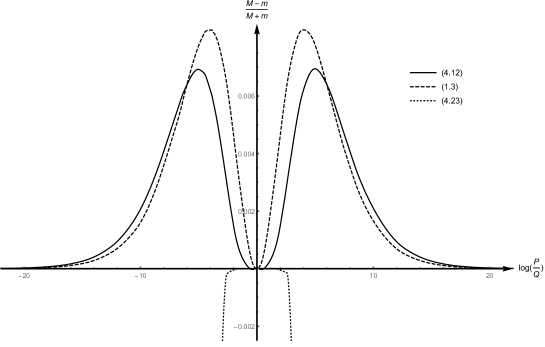
Figure 1: This plot shows the difference between the approximate mass formula $M$ and the actual mass $m$ obtained from the numerical calculations, with horizontal axis $x=\log(P/Q)$ and vertical axis $y=(M-m)/(M+m)$. In this plot, we fix $PQ=1/8$, corresponding to a horizon radius $r_{0}=1$. The dashed line is from the Rasheed formula, the continuous line is for our new formula (4.21); the dotted line for (4.34). Thus for $|\log(P/Q)|<2$, the mass formula (4.34) is much better, but it quickly diverges from the true mass as $|\log(P/Q)|$ increases, with a radius of convergence of about 2. Our new formula (4.21) is better than Rasheed’s at small $x$, but is not as good as $x$ increases. However, overall our expression (4.21) appears to improve upon Rasheed’s in fitting the actual data. The maximum error in our formula is about 0.6%, whilst Rasheed’s is about 0.9%. We also obtained similar results for the case $a=\sqrt{10}$.

5 Entropy super-additivity and sub-additivity

As we discussed in the introduction, entropy super-additivity is a property exhibited by many black holes, although the dyonic black hole in the $a=\sqrt{3}$ EMD theory provides a counter-example [14]. Since the dyonic black holes in $a=0$ and $a=1$ EMD theory do, on the other hand, obey the super-additivity property, it is therefore of interest to study for general values of the dilaton coupling $a$.

For a static black hole with mass $M$ and electric and magnetic charges $Q$ and $P$, the entropy must be a function of these quantities,

$$S=S(M,Q,P)\,.$$ (5.1)

We now consider the splitting of the black hole into two black holes with masses and charges $(M_{1},Q_{1},P_{1})$ and $(M_{2},Q_{2},P_{2})$, with

$$M=M_{1}+M_{2}\,,\qquad Q=Q_{1}+Q_{2}\,,\qquad P=P_{1}+P_{2}\,,$$ (5.2)

and we consider the quantity

$$\Delta S\equiv S(M,Q,P)-S(M_{1},Q_{1},P_{1})-S(M_{2},Q_{2},P_{2})\,.$$ (5.3)

The splitting of the black hole is the inverse of the joining of the two black holes, and the entropy is super-additive if $\Delta S>0$, and sub-additive if $\Delta S<0$.

Our goal in this section is to study $\Delta S$ in cases where a non-trivial dyonic black hole with $Q\neq P$ is involved, and in the earlier sections we have obtained approximate results for such black holes in the case of the extremal limit. Thus here, we shall investigate the entropy additivity property for the splitting of an extremal dyonic black hole with mass $M$ and electric and magnetic charges $(Q,P)$ into two black holes where one is purely electric, with mass $M_{1}$ and charge $(Q,0)$, and the other is purely magnetic, with mass $M_{2}$ and charge $(0,P)$. These purely electric and magnetic black holes are not necessarily extremal. Since we require $M=M_{1}+M_{2}$, and since $M_{1}$ and $M_{2}$ are bounded below by the masses $M_{1}(Q,0)_{\rm ext}$ and $M_{2}(0,P)_{\rm ext}$ of the extremal black holes with these charges,

$$M_{1}(Q,0)\geq M_{1}(Q,0)_{\rm ext}\,,\qquad M_{2}(0,P)\geq M_{2}(0,P)_{\rm ext}\,,$$ (5.4)

it follows that we must have

$$M(Q,P)_{\rm ext}\geq M(Q,0)_{\rm ext}+M(0,P)_{\rm ext}\,.$$ (5.5)

The dyonic black holes satisfying this condition have been referred to as “black hole bombs” [20, 21]. They are closely related to the $SL(3,R)$-Toda system and can be generalized to $SL(n,R)$-Toda black holes [22].

In the following subsections, we shall study $\Delta S$ as a function of the dilaton coupling $a$ in two situations; in one, $Q$ and $P$ will be held fixed, whilst in the other we shall hold the entropy $S=8\pi PQ$ of the extremal dyonic black hole fixed, and look at $\Delta S$ as the ratio $P/Q$ is allowed to vary.

5.1 Fixed $P$ and $Q$

We shall first study the simple case where $Q=P$, for which the mass of the extremal dyonic black hole is known exactly (see section 3.2, under eqn (3.7)):

$$M=M(Q,Q)_{\rm ext}=2\sqrt{2}Q\,,\qquad S(Q,Q)_{\rm ext}=8\pi Q^{2}\,.$$ (5.6)

The masses $M_{1}=M_{1}(Q,0)$ and $M_{2}=M_{2}(0,Q)$ of the purely electric and purely magnetic black holes must satisfy $M_{1}+M_{2}=M=2\sqrt{2}Q$. Thus $M_{1}$ must satisfy

$${\frac{2}{\sqrt{a^{2}+1}}}Q=M_{1}^{\rm ext}\leq M_{1}=M-M_{2}\leq M-M_{2}^{\rm ext}=2\sqrt{2}Q-{\frac{2}{\sqrt{a^{2}+1}}}Q\,.$$ (5.7)

Note that from the inequality between the left-most and right-most terms in this expression, we can immediately deduce that we must have $a\geq 1$. The entropy of the two electric and magnetically charged black holes are given in (3.4). We can thus evaluate $\Delta S$ as a function of $M_{1}$, for various values of the dilaton coupling constant $a$. Setting $Q=1$ without loss of generality, these results are plotted in the left-hand graph in Fig. 2, for the examples of $a^{2}=3$, 6 and 10.

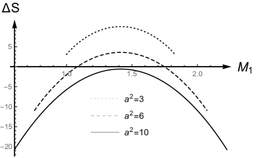
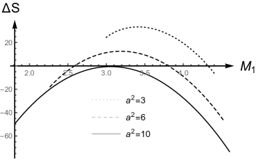
Figure 2: In both plots, we present $\Delta S$ as a function of $M_{1}$, which runs from $M_{1}^{\rm ext}$ to $M-M_{2}^{\rm ext}$, for the cases $a^{2}=3$, 6 and 10. In the left-hand plot we have chosen $Q=P=1$, and in the right-hand plot $Q=3,P=1$.

We now turn to an example where $Q$ and $P$ are unequal. For generic values of $a$, this means that we must resort to numerical methods to construct the extremal dyonic solution. We shall consider the example where $Q=3$ and $P=1$. In this case, the purely electric and magnetic solutions are

$$M_{1}^{\rm ext}={\frac{6}{\sqrt{a^{2}+1}}}\,,\qquad M_{2}^{\rm ext}={\frac{2}{\sqrt{a^{2}+1}}}\,.$$ (5.8)

The masses of the dyonic solutions for $a^{2}=6,10$ cases have to be obtained by numerical methods, described in appendix B. We find

$$a^{2}=3: M=(1+3^{{\frac{2}{3}}})^{{\frac{3}{2}}}\sim 5.41\,,$$

$$a^{2}=6: M\sim 5.28\,,$$

$$a^{2}=10: M\sim 5.20\,.$$ (5.9)

With these data, we can calculate $\Delta S$ as a function of $M_{1}$, which runs from $M_{1}^{\rm ext}$ to $M-M_{2}^{\rm ext}$. The result is presented in the right-hand graph in Fig. 2.

The general picture that emerges from these examples is that in this region of parameter space the entropy is super-additive for small values of $a^{2}$, but it tends to become sub-additive for larger values of $a^{2}$.

5.2 Fixed $S_{P,Q}=8\pi PQ$

Here, we study the super-additivity of the entropy for the splitting an extremal dyonic black hole into an extremal magnetically-charged black hole and a non-extremal electrically-charged black hole. We look at $\Delta S$ as a function of the ratio $P/Q$ while holding the entropy of the extremal dyonic black hole fixed. In particular we shall consider a horizon radius $r_{0}=1$ for the extremal dyonic black hole. In other words, it will have $S=\pi$ and $PQ=1/8$. Since the entropy $S_{\rm P}^{\rm ext}$ for the extremal magnetically-charged black hole vanishes, we shall have

$$\Delta S=S_{\rm P,Q}^{\rm ext}-S_{Q}^{\rm non-ext}\,.$$ (5.10)

We obtain and plot the results, again for the cases $a^{2}=3$, 6 and 10, in Fig. 3. The result for $a^{2}=3$ can be obtained analytically. For the cases $a^{2}=6$ and $a^{2}=10$, we have used the numerical solutions to find the mass.

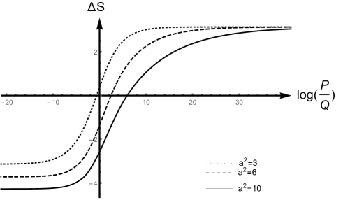
Figure 3: The entropy difference for splitting a dyonic black hole to an extremal magnetic black hole and a non-extremal electric black hole. The electric and magnetic charges satisfy $QP=1/8$. The entropy is super-additive for sufficiently large $P/Q$ and becomes sub-additive as $P/Q$ decreases. Note that for all the $a^{2}=3$, 6 and 10 cases, the extremal dyonic black hole can be viewed as a black hole bomb, satisfying (5.5).

First, we note that for large $P/Q$, the quantity $\Delta S$ is positive and hence the entropy is super-additive. As $P/Q$ decreases, $\Delta S$ becomes negative, and so the entropy becomes sub-additive. Interestingly, in the limit $P/Q\rightarrow 0$, the quantity $\Delta S$ approaches a negative constant that depends on $a$. Assuming this conclusion is in general true for the $a^{2}\geq 1$ cases, we can derive some useful information about the mass of the dyonic black hole as $P/Q\rightarrow 0$. It is evident that at leading order, the mass in this limit is given by $\sqrt{N}Q$. We postulate that the sub-leading order is given by

$$M=\sqrt{N}Q\Big{(}1+\gamma\,\big{(}{\frac{P}{Q}}\big{)}^{\delta}+\cdots\Big{)}\,,\qquad\hbox{with}\qquad{\frac{P}{Q}}\rightarrow 0\,.$$ (5.11)

Here $(\delta,\gamma)$ are constants that at present we are unable to determine for the case of a generic dilaton coupling constant $a$. After the dyonic black hole is split into purely electric and purely magnetic black holes, only the non-extremal electric black hole has an entropy. The mass of the electric black hole is

$$M_{Q}=\sqrt{N}Q\Big{(}1+\gamma\,\big{(}{\frac{P}{Q}}\big{)}^{\delta}-{\frac{P}{Q}}+\cdots\Big{)}\,.$$ (5.12)

Assuming that $\delta<1$, it then follows from (3.4) that at leading order the entropy is given by

$$S_{Q}^{\rm non-ext}=\pi(1+a^{2})2^{2{\frac{1+2a^{2}}{1+a^{2}}}}a^{-{\frac{4a^{2}}{1+a^{2}}}}\big{(}\gamma{\frac{P}{Q}}\big{)}^{{\frac{2a^{2}}{1+a^{2}}}}Q^{2}+\cdots\,.$$ (5.13)

Since $PQ$ is fixed, for this leading-order quantity to be constant we must have

$$\delta={\frac{1+a^{2}}{2a^{2}}}\,.$$ (5.14)

Note that $\delta\leq 1$ for $a^{2}\geq 1$, thus the result is applicable for $a^{2}>1$. Then, at leading order as $P/Q\rightarrow 0$, $\Delta S$ is given by

$$\Delta S\rightarrow 8\pi PQ(1-c)\,,\qquad c=(1+a^{2})2^{{\frac{a^{2}-1}{a^{2}+1}}}a^{-{\frac{4a^{2}}{a^{2}+1}}}\gamma^{{\frac{2a^{2}}{a^{2}+1}}}\,.$$ (5.15)

For the special case $a^{2}=3$, we have $\delta=2/3$ and $\gamma=3/2$, and hence $c=2$. This is consistent with the $a=\sqrt{3}$ result in Fig. 3. For general $a>1$, we have determined $\delta$ by this method, but the coefficient $\gamma$ cannot be determined generically. The plots indicates that the constant $c$ is bigger than 1 and it increases as $a$ increases.

6 Conclusions

In this paper, we have studied the extremal static dyonic solutions of the four-dimensional Einstein-Maxwell-Dilaton theory for generic values of the dilaton coupling $a$. Except in the special cases $a=0$, $a=1$ and $a=\sqrt{3}$, where the explicit solutions can be constructed, it is necessary to use approximation techniques or numerical methods in order to study the solutions.

Our method for constructing approximate solutions is based on the observation that one can solve the equations explicitly, for any value of $a$, in the special case when the electric charge $Q$ and the magnetic charge $P$ are equal. (The dilaton becomes constant in this case, and the solution is just an extremal Reissner-Nordström $Q=P$ dyonic black hole.) We then construct the solution, in terms of series expansions in powers of the small parameter $\epsilon=a^{-1}\,\log(Q/P)$, in the regime where the ratio $Q/P$ is close to unity.

One of our reasons for studying this problem is that there is a long-standing conjecture by Rasheed [11], dating back to 1995, for a possible expression for the mass of the extremal dyonic black hole as a function of the electric and magnetic charges and the dilaton coupling $a$. The power-series solutions that we obtain for $Q/P$ close to unity are sufficient to be able to demonstrate that the conjectured mass formula in [11] fails, at order $\epsilon^{2}$, when $a$ is not equal to one of the three values mentioned above for which the exact dyonic solutions are known. We were able to show, however, by means of a numerical construction of the dyonic solutions, that the conjectured mass formula is a reasonably good approximation even as one moves away from the $Q\sim P$ regime of our power-series solutions. We have also made some somewhat improved conjectures for mass formulae, which work up to higher orders in $\epsilon$, but again, they are only approximations. However, our findings from the numerical construction of the dyonic black hole solutions suggest that both the Rasheed formula (1.5) and our formula (4.21) capture the essence of the mass-charge relation for extremal dyonic black holes quite accurately, even when $Q/P$ is far away from unity.

Our perturbative construction of the extremal dyonic black hole solutions made use of the fact that we know the exact solution, for all $a$, when $Q=P$, and so we could expand around this solution in terms of the small parameter $\epsilon=a^{-1}\,\log(Q/P)$. Of course, we also know the exact solution when $P=0$ or $Q=0$, and one might wonder whether this could provide another starting point for obtaining a solution as a perturbative expansion valid for very large $P/Q$ or $Q/P$. However, this does not seem to be a promising option. The problem is that no matter how large or small $Q/P$ is, as long as $Q$ and $P$ are both non-zero the near-horizon geometry of the extremal black hole is of the form AdS${}_{2}\times S^{2}$. By contrast, the horizon is singular for an extremal black hole carrying purely electric or purely magnetic charge (except in the case $a=0$). Thus the starting point for such a perturbative expansion would be singular. It is interesting, nevertheless, that our numerical construction of the black hole solutions led us to a mass formula of the form (5.11) for a nearly electric extremal black hole, with $\delta$ given by (5.14).

The other main topic in this paper has been the study of the circumstances under which the property of super-additivity of the entropy of the dyonic black holes is satisfied. This property, defined in our discussion in the introduction, has been found to be satisfied by many classes of black hole solutions. But already, in [14], it was observed that it could be violated in certain regimes for dyonic $a=\sqrt{3}$ EMD black holes. Our findings in this paper extend this observation further, and indicate that entropy super-additivity can be violated in certain parameter regimes for all the dyonic EMD black holes with larger values of $a$.

All the examples where entropy super-additivity fails are associated with the situation where a “black-hole bomb” can occur, of the kind discussed for $a=\sqrt{3}$ extremal dyonic black holes in [20, 21]. Namely, these are situations where the mass of an extremal dyonic black hole is greater than the sums of the masses of separated pure electric and pure magnetic black holes of the same total charge, as in (5.5). This can happen, as we saw, when the dilaton coupling $a$ is such that $a^{2}>1$.

In [14], the relation between Hawking’s black hole area theorem and entropy super-additivity was discussed. The area theorem asserts that, subject to cosmic censorship, the area (or entropy) of the horizon of a black hole final state formed from the coalescence of two black holes cannot be less than the sum of the two original horizon areas (or entropies). The area theorem would then imply entropy super-additivity [14]. However, an important distinction is that the area theorem is only applicable in cases where the coalescence of the black holes is physically possible. As discussed in [12] for the $a=\sqrt{3}$ dyonic black hole, if a static dyonic black hole separated into a pure electric and a pure magnetic black hole, there would be an angular momentum proportional to $QP$ and so the decay to purely static constituents would seem to be ruled out by angular momentum conservation. Thus the breakdown of entropy super-additivity that we have seen in cases where $a^{2}>1$ in this paper need not be in conflict with the Hawking area theorem.

An intriguing point, worthy of further investigation, is that one can seemingly sidestep the complication of angular momentum in the electromagnetic field of a decomposed dyonic black hole by considering a slight modification of the original EMD theory (1.1), in which a second electromagnetic field is introduced, with the Lagrangian

$${\cal L}=\sqrt{-g}(R-{\textstyle{\frac{\scriptstyle 1}{\scriptstyle 2}}}(\partial\phi)^{2}-{\textstyle{\frac{\scriptstyle 1}{\scriptstyle 4}}}e^{a\phi}F_{1}^{2}-{\textstyle{\frac{\scriptstyle 1}{\scriptstyle 4}}}e^{-a\phi}F_{2}^{2}\,.$$ (6.1)

This theory admits black hole solutions where $F_{1}$ and $F_{2}$ carry electric charges $Q_{1}$ and $Q_{2}$ that are essentially identical to the dyonic solutions of the EMD theory (1.1), where the EMD charges are $Q=Q_{1}$ and $P=Q_{2}$ [23]. One then has all the same features of the occurrence of black-hole bomb solutions for $a^{2}>1$, and violations of entropy super-additivity, as we saw earlier in the EMD theory. Now, however, there is no angular momentum in the electromagnetic field(s) for separated component black holes, and so the argument in [12] that could have ruled out the dyon decay process no longer applies. It would be interesting to investigate this further, to see how the occurrence of entropy sub-additivity could be compatible with the Hawking area theorem for the black holes in this theory.

Appendix A Approximate solution up to $\epsilon^{10}$ order

In this appendix, we present the dyonic extremal black hole solution (4.6) up to and including the order $\epsilon^{10}$. The results are necessary to derive the mass formula (4.18). Having defined (4.11), we have

$${\frac{h}{x^{2}}} = 1+\epsilon^{2}\frac{k\left(x-x^{2k}\right)}{4(1-2k)x}+\frac{\epsilon^{4}k^{2}}{192\left(16k^{2}-1\right)(1-2k)^{2}x^{2}}\Big{(}2\left(4k^{4}+8k^{3}+45k^{2}+4k-1\right)x^{2}$$ (A.76)

$$+3(1-2k)^{2}\left(2k^{2}-12k-5\right)x^{4k+1}-4\left(8k^{4}+10k^{3}+57k^{2}+5k-5\right)x^{2k+1}$$

$$+3(4k-1)(4k+1)^{2}x^{4k}\Big{)}$$

$$-\frac{\epsilon^{6}k^{3}}{23040(2k-1)^{3}(4k-1)(4k+1)^{2}(6k-1)(6k+1)x^{3}}\Big{[}$$

$$-45(2k-1)^{2}(4k+1)(6k-1)(6k+1)^{2}\left(2k^{2}-12k-5\right)x^{6k+1}$$

$$+30(4k-1)(4k+1)^{2}(6k-1)(6k+1)\left(4k^{3}+6k^{2}+18k+7\right)x^{4k+1}$$

$$+30(2k-1)^{2}(6k-1)(6k+1)\left(2k^{2}-12k-5\right)\left(4k^{3}+6k^{2}+18k+7\right)x^{4k+2}$$

$$-45(2k-1)^{3}(4k-1)\left(12k^{5}-168k^{4}+384k^{3}+478k^{2}+154k+15\right)x^{6k+2}$$

$$-4(6k-1)\Big{(}816k^{8}+2596k^{7}+10976k^{6}+17565k^{5}+30794k^{4}$$

$$+16852k^{3}+1980k^{2}-638k-91\Big{)}x^{2k+2}+4\Big{(}576k^{9}+2880k^{8}$$

$$+10040k^{7}+18424k^{6}+35874k^{5}+16588k^{4}+4178k^{3}+657k^{2}+32k+1\Big{)}x^{3}$$

$$90k(4k-1)(4k+1)^{2}(6k-1)(6k+1)^{2}x^{6k}\Big{]}$$

$$+\frac{\epsilon^{8}k^{4}}{5160960(1-4k)^{2}(4k+1)^{3}\left(2304k^{4}-100k^{2}+1\right)(1-2k)^{4}x^{4}}\Big{[}$$

$$840k(4k-1)^{2}(4k+1)^{3}(6k-1)(6k+1)(8k-1)^{2}(8k+1)^{2}x^{8k}$$

$$-32(4k-1)(8k-1)\Big{(}142848k^{13}+739008k^{12}+3101104k^{11}+7958032k^{10}$$

$$+16656424k^{9}+23696532k^{8}+26928519k^{7}+18001947k^{6}+6125349k^{5}$$

$$+688362k^{4}-88674k^{3}-2111k^{2}+2455k+205\Big{)}x^{2k+3}$$

$$+504(4k-1)(4k+1)^{2}(6k-1)(8k-1)(8k+1)\Big{(}288k^{8}+888k^{7}+2808k^{6}$$

$$+4150k^{5}+5382k^{4}+3066k^{3}+395k^{2}-154k-23\Big{)}x^{4k+2}$$

$$+504(2k-1)^{2}(6k-1)(8k-1)(8k+1)\left(2k^{2}-12k-5\right)\Big{(}288k^{8}+888k^{7}$$

$$+2808k^{6}+4150k^{5}+5382k^{4}+3066k^{3}+395k^{2}-154k-23\Big{)}x^{4k+3}$$

$$-5040k(2k+1)(4k-1)^{2}(4k+1)^{2}(6k-1)(6k+1)^{2}(8k-1)(8k+1)$$

$$\times\left(k^{2}+k+3\right)x^{6k+1}-2520(2k-1)^{2}(2k+1)(4k-1)(4k+1)(6k-1)$$

$$\times(6k+1)^{2}(8k-1)(8k+1)\left(k^{2}+k+3\right)\left(2k^{2}-12k-5\right)x^{6k+2}$$

$$-2520(2k-1)^{3}(2k+1)(4k-1)^{2}(8k-1)(8k+1)\left(k^{2}+k+3\right)$$

$$\times\left(12k^{5}-168k^{4}+384k^{3}+478k^{2}+154k+15\right)x^{6k+3}$$

$$+5040k(2k-1)^{2}(4k-1)(4k+1)^{2}(6k-1)(6k+1)(8k-1)(8k+1)^{2}$$

$$\times\left(2k^{2}-12k-5\right)x^{8k+1}+315(2k-1)^{3}(4k+1)(8k-1)(8k+1)^{2}$$

$$\times\left(1056k^{7}-14736k^{6}+40648k^{5}+21908k^{4}-6720k^{3}-3072k^{2}+206k+85\right)x^{8k+2}$$

$$+105(2k-1)^{4}(4k-1)^{2}(4k+1)(6k-1)\Big{(}288k^{7}-6816k^{6}+41288k^{5}-42780k^{4}$$

$$-98488k^{3}-49044k^{2}-9238k-585\Big{)}x^{8k+3}+8\Big{(}1253376k^{15}+10708992k^{14}$$

$$+36770816k^{13}+94049792k^{12}+188965248k^{11}+274829056k^{10}+333916576k^{9}$$

$$+198513792k^{8}+76889376k^{7}+16710012k^{6}-958500k^{5}-1023835k^{4}-208600k^{3}$$

$$-25410k^{2}-692k+1\Big{)}x^{4}\Big{]}$$

$$+\frac{\epsilon^{10}k^{5}/1857945600}{(1-4k)^{2}(2k-1)^{5}(4k+1)^{4}(6k-1)(6k+1)^{2}((8k)^{2}-1)((10k)^{2}-1)x^{5}}\Big{[}$$

$$18900k(4k+1)^{4}(5k-1)(6k-1)(6k+1)^{2}(8k-1)(8k+1)(10k+1)^{2}(1-4k)^{2}$$

$$\times(1-10k)^{2}x^{10k}+16(10k-1)\Big{(}24454103040k^{20}+180194770944k^{19}$$

$$+818173599744k^{18}+2620475621888k^{17}+6424614622720k^{16}+12257466595232k^{15}$$

$$+18895354632528k^{14}+22768387442448k^{13}+21525540388776k^{12}$$

$$+14557877561170k^{11}+6343842768089k^{10}+1440749945746k^{9}-16416399844k^{8}$$

$$-81249938138k^{7}-13005568630k^{6}-2134737402k^{5}-422081208k^{4}-38850528k^{3}$$

$$-1452596k^{2}+118640k+7381\Big{)}x^{2k+4}-240(4k-1)(4k+1)^{2}(6k+1)$$

$$\times(8k-1)(10k-1)(10k+1)\Big{(}1953792k^{13}+9522432k^{12}+33807040k^{11}$$

$$+77129152k^{10}+137796448k^{9}+176370384k^{8}+170812668k^{7}+107973084k^{6}$$

$$+35323968k^{5}+1927524k^{4}-1522824k^{3}-84773k^{2}+27358k+2497\Big{)}x^{4k+3}$$

$$-240(1-2k)^{2}(6k+1)(8k-1)(10k-1)(10k+1)\left(2k^{2}-12k-5\right)\Big{(}1953792k^{13}$$

$$+9522432k^{12}+33807040k^{11}+77129152k^{10}+137796448k^{9}+176370384k^{8}$$

$$+170812668k^{7}+107973084k^{6}+35323968k^{5}+1927524k^{4}-1522824k^{3}$$

$$-84773k^{2}+27358k+2497\Big{)}x^{4k+4}+15120k(4k-1)(4k+1)^{2}(6k-1)$$

$$\times(6k+1)^{2}(8k-1)(8k+1)(10k-1)(10k+1)\Big{(}1776k^{8}+5396k^{7}+14776k^{6}$$

$$+20945k^{5}+23464k^{4}+13512k^{3}+1880k^{2}-778k-121\Big{)}x^{6k+2}$$

$$+7560(4k+1)(6k-1)(6k+1)^{2}(8k-1)(8k+1)(10k-1)(10k+1)(1-2k)^{2}$$

$$\times\left(2k^{2}-12k-5\right)\Big{(}1776k^{8}+5396k^{7}+14776k^{6}+20945k^{5}+23464k^{4}+13512k^{3}$$

$$+1880k^{2}-778k-121\Big{)}x^{6k+3}+7560(2k-1)^{3}(4k-1)(8k-1)(8k+1)(10k-1)$$

$$\times(10k+1)\left(12k^{5}-168k^{4}+384k^{3}+478k^{2}+154k+15\right)\Big{(}1776k^{8}+5396k^{7}$$

$$+14776k^{6}+20945k^{5}+23464k^{4}+13512k^{3}+1880k^{2}-778k-121\Big{)}x^{6k+4}$$

$$-25200(1-8k)^{2}(1-4k)^{2}k(4k+1)^{3}(6k-1)(6k+1)^{2}(8k+1)^{2}(10k-1)$$

$$\times(10k+1)\left(8k^{3}+12k^{2}+24k+11\right)x^{8k+1}-151200(1-2k)^{2}k(4k-1)(4k+1)^{2}$$

$$\times(6k-1)(6k+1)^{2}(8k-1)(8k+1)^{2}(10k-1)(10k+1)\left(2k^{2}-12k-5\right)$$

$$\times\left(8k^{3}+12k^{2}+24k+11\right)x^{8k+2}-9450(2k-1)^{3}(4k+1)(6k+1)(8k-1)$$

$$\times(8k+1)^{2}(10k-1)(10k+1)\left(8k^{3}+12k^{2}+24k+11\right)\Big{(}1056k^{7}-14736k^{6}$$

$$+40648k^{5}+21908k^{4}-6720k^{3}-3072k^{2}+206k+85\Big{)}x^{8k+3}-3150(1-4k)^{2}$$

$$\times(1-2k)^{4}(4k+1)(6k-1)(6k+1)(10k-1)(10k+1)\left(8k^{3}+12k^{2}+24k+11\right)$$

$$\times\left(288k^{7}-6816k^{6}+41288k^{5}-42780k^{4}-98488k^{3}-49044k^{2}-9238k-585\right)x^{8k+4}$$

$$+94500k(4k-1)(4k+1)^{3}(6k-1)(6k+1)^{2}(8k-1)(8k+1)(10k+1)^{2}(1-2k)^{2}$$

$$\times(1-10k)^{2}\left(2k^{2}-12k-5\right)x^{10k+1}+141750k(2k-1)^{3}(4k+1)^{2}(6k+1)(8k-1)$$

$$\times(8k+1)(10k-1)(10k+1)^{2}\Big{(}672k^{7}-9168k^{6}+25648k^{5}+13092k^{4}-4768k^{3}$$

$$-2044k^{2}+138k+55\Big{)}x^{10k+2}+4725(4k-1)(4k+1)(6k+1)(10k-1)(10k+1)^{2}$$

$$\times(1-2k)^{4}\Big{(}46080k^{10}-1036800k^{9}+6347040k^{8}-7926032k^{7}-13623936k^{6}$$

$$-3194472k^{5}+1403580k^{4}+601032k^{3}+30696k^{2}-10528k-1035\Big{)}x^{10k+3}$$

$$+4725(2k-1)^{5}(4k+1)(6k-1)(8k-1)(1-4k)^{2}\Big{(}17280k^{11}-586800k^{10}$$

$$+5939232k^{9}-19042592k^{8}-2829296k^{7}+47470368k^{6}+51882672k^{5}+24555420k^{4}$$

$$+6245400k^{3}+885440k^{2}+65762k+1989\Big{)}x^{10k+4}-16\Big{(}10970726400k^{21}$$

$$+146040422400k^{20}+641482899456k^{19}+1856477659136k^{18}+4318539487232k^{17}$$

$$+8304191960320k^{16}+13318866483328k^{15}+17499377526912k^{14}$$

$$+18755721158592k^{13}+15109498274704k^{12}+9239954852200k^{11}$$

$$+4215820540256k^{10}+1343741413744k^{9}+260198810504k^{8}+18391021108k^{7}$$

$$-6289646720k^{6}-2254086318k^{5}-335839017k^{4}-29710472k^{3}$$

$$-1578494k^{2}-25270k-1\Big{)}x^{5}\Big{]}\,,$$

and also

$$\phi = \epsilon(1-x^{k})-\frac{\epsilon^{3}kx^{k-1}}{24\left(8k^{2}-2k-1\right)}\Big{[}\left(2k^{3}-9k^{2}+2\right)x^{2k+1}+3k(4k+1)x^{2k}$$ (A.136)

$$-\left(2k^{3}+3k^{2}+3k+2\right)x\Big{]}-\frac{\epsilon^{5}k^{2}x^{k-2}}{1920\left(-8k^{2}+2k+1\right)^{2}\left(24k^{2}-2k-1\right)}\Big{[}$$

$$-30k(k+1)(4k-1)(4k+1)(6k+1)\left(2k^{2}+k+2\right)x^{2k+1}-10(k+1)(2k-1)$$

$$\times(4k-1)(6k+1)\left(k^{2}-4k-2\right)\left(2k^{2}+k+2\right)x^{2k+2}+45k(2k-1)(4k+1)$$

$$\times(6k+1)\left(4k^{3}-20k^{2}-2k+3\right)x^{4k+1}+3(4k-1)(4k+1)(1-2k)^{2}$$

$$\times\left(3k^{4}-34k^{3}+60k^{2}+64k+12\right)x^{4k+2}+(k+1)\Big{(}384k^{7}+880k^{6}+844k^{5}$$

$$+1196k^{4}+495k^{3}+433k^{2}-28k-4\Big{)}x^{2}+15k(4k-1)(4k+1)^{2}(5k-1)$$

$$\times(6k+1)x^{4k}\Big{]}-\frac{\epsilon^{7}k^{3}x^{k-3}}{322560\left(8k^{2}-2k-1\right)^{3}\left(24k^{2}-10k+1\right)\left(48k^{2}+14k+1\right)}\Big{[}$$

$$-525k(k+1)(4k-1)(4k+1)^{2}(5k-1)(6k-1)(6k+1)(8k+1)$$

$$\times\left(2k^{2}+k+2\right)x^{4k+1}-1575k(k+1)(2k-1)(4k+1)(6k-1)(6k+1)(8k+1)$$

$$\times\left(2k^{2}+k+2\right)\left(4k^{3}-20k^{2}-2k+3\right)x^{4k+2}+315k(2k-1)(4k+1)^{2}(6k-1)$$

$$\times(6k+1)(7k-1)(8k+1)\left(8k^{3}-43k^{2}-2k+7\right)x^{6k+1}-105(1-2k)^{2}(k+1)$$

$$\times(4k-1)(4k+1)(6k-1)(8k+1)\left(2k^{2}+k+2\right)\left(3k^{4}-34k^{3}+60k^{2}+64k+12\right)$$

$$\times x^{4k+3}+21k(k+1)(4k+1)(6k-1)(8k+1)\Big{(}2112k^{7}+4480k^{6}+5452k^{5}$$

$$+6368k^{4}+3015k^{3}+1969k^{2}-244k-52\Big{)}x^{2k+2}+7(k+1)(2k-1)(6k-1)$$

$$\times(8k+1)\left(k^{2}-4k-2\right)\Big{(}2112k^{7}+4480k^{6}+5452k^{5}+6368k^{4}+3015k^{3}+1969k^{2}$$

$$-244k-52\Big{)}x^{2k+3}+315k(4k+1)(8k+1)(1-2k)^{2}\Big{(}528k^{7}-6240k^{6}+13902k^{5}$$

$$+8549k^{4}-2480k^{3}-1251k^{2}+80k+37\Big{)}x^{6k+2}+15(2k-1)^{3}(4k-1)(4k+1)$$

$$\times(6k-1)\left(72k^{7}-1449k^{6}+7162k^{5}-4290k^{4}-14972k^{3}-8316k^{2}-1712k-120\right)$$

$$\times x^{6k+3}+105k(4k-1)(4k+1)^{3}(6k-1)(6k+1)(7k-2)(7k-1)(8k+1)x^{6k}$$

$$-(k+1)\Big{(}313344k^{12}+1416960k^{11}+2031488k^{10}+2659344k^{9}+3369536k^{8}$$

$$+2520904k^{7}+2329376k^{6}+866389k^{5}+542126k^{4}+2059k^{3}+13622k^{2}$$

$$-156k+8\Big{)}x^{3}\Big{]}$$

$$-\frac{\epsilon^{9}k^{4}x^{k-4}/92897280}{\left(-24k^{2}+2k+1\right)^{2}\left(-8k^{2}+2k+1\right)^{4}\left(3840k^{4}-256k^{3}-124k^{2}+4k+1\right)}\Big{[}$$

$$2835k(3k-1)(4k+1)^{4}(6k-1)(6k+1)^{2}(8k-1)(8k+1)(9k-2)(9k-1)$$

$$\times(10k+1)(1-4k)^{2}x^{8k}-60k(k+1)(4k-1)(4k+1)(6k+1)(8k-1)(10k+1)$$

$$\times\Big{(}1622016k^{12}+6469632k^{11}+11055040k^{10}+15928848k^{9}+17757472k^{8}$$

$$+14360408k^{7}+10484068k^{6}+4008509k^{5}+1687990k^{4}-210673k^{3}-6314k^{2}$$

$$+2676k+328\Big{)}x^{2k+3}-20(k+1)(2k-1)(4k-1)(6k+1)(8k-1)$$

$$\times(10k+1)\left(k^{2}-4k-2\right)\Big{(}1622016k^{12}+6469632k^{11}+11055040k^{10}$$

$$+15928848k^{9}+17757472k^{8}+14360408k^{7}+10484068k^{6}+4008509k^{5}$$

$$+1687990k^{4}-210673k^{3}-6314k^{2}+2676k+328\Big{)}x^{2k+4}+630k(k+1)(4k-1)$$

$$\times(4k+1)^{2}(5k-1)(6k-1)(6k+1)(8k-1)(8k+1)(10k+1)\Big{(}3072k^{7}$$

$$+6320k^{6}+8372k^{5}+9148k^{4}+4545k^{3}+2639k^{2}-404k-92\Big{)}x^{4k+2}$$

$$+1890k(k+1)(2k-1)(4k+1)(6k-1)(6k+1)(8k-1)(8k+1)(10k+1)$$

$$\times\left(4k^{3}-20k^{2}-2k+3\right)\Big{(}3072k^{7}+6320k^{6}+8372k^{5}+9148k^{4}+4545k^{3}$$

$$+2639k^{2}-404k-92\Big{)}x^{4k+3}+126(k+1)(4k-1)(4k+1)(6k-1)(8k-1)$$

$$\times(8k+1)(10k+1)(1-2k)^{2}\left(3k^{4}-34k^{3}+60k^{2}+64k+12\right)\Big{(}3072k^{7}$$

$$+6320k^{6}+8372k^{5}+9148k^{4}+4545k^{3}+2639k^{2}-404k-92\Big{)}x^{4k+4}$$

$$-8820(1-4k)^{2}k(k+1)(4k+1)^{3}(6k-1)(6k+1)^{2}(7k-2)(7k-1)(8k-1)$$

$$\times(8k+1)(10k+1)\left(2k^{2}+k+2\right)x^{6k+1}-26460k(k+1)(2k-1)(4k-1)$$

$$\times(4k+1)^{2}(6k-1)(6k+1)^{2}(7k-1)(8k-1)(8k+1)(10k+1)\left(2k^{2}+k+2\right)$$

$$\times\left(8k^{3}-43k^{2}-2k+7\right)x^{6k+2}-26460(1-2k)^{2}k(k+1)(4k-1)(4k+1)$$

$$\times(6k+1)(8k-1)(8k+1)(10k+1)\left(2k^{2}+k+2\right)\Big{(}528k^{7}-6240k^{6}+13902k^{5}$$

$$+8549k^{4}-2480k^{3}-1251k^{2}+80k+37\Big{)}x^{6k+3}-1260(1-4k)^{2}(k+1)(2k-1)^{3}$$

$$\times(4k+1)(6k-1)(6k+1)(8k-1)(10k+1)\left(2k^{2}+k+2\right)\Big{(}72k^{7}-1449k^{6}$$

$$+7162k^{5}-4290k^{4}-14972k^{3}-8316k^{2}-1712k-120\Big{)}x^{6k+4}+1890k(2k-1)$$

$$\times(4k-1)(4k+1)^{3}(6k-1)(6k+1)^{2}(8k-1)(8k+1)(9k-2)(9k-1)(10k+1)$$

$$\times\left(20k^{3}-112k^{2}-2k+19\right)x^{8k+1}+2835k(4k+1)^{2}(6k+1)(8k-1)(8k+1)$$

$$\times(9k-1)(10k+1)(1-2k)^{2}\Big{(}6720k^{8}-82368k^{7}+215376k^{6}+48524k^{5}$$

$$-70874k^{4}-5716k^{3}+6472k^{2}+140k-149\Big{)}x^{8k+2}+2835k(2k-1)^{3}(4k-1)$$

$$\times(4k+1)(6k+1)(10k+1)\Big{(}153600k^{11}-3068928k^{10}+16559680k^{9}-17930416k^{8}$$

$$-28325608k^{7}-1887768k^{6}+4959928k^{5}+865666k^{4}-224292k^{3}-45844k^{2}$$

$$+2762k+595\Big{)}x^{8k+3}+315(4k+1)(6k-1)(6k+1)(8k-1)(1-2k)^{4}(1-4k)^{2}$$

$$\times\Big{(}960k^{10}-28904k^{9}+255619k^{8}-687148k^{7}-248660k^{6}+1424192k^{5}+1520776k^{4}$$

$$+645008k^{3}+135520k^{2}+13952k+560\Big{)}x^{8k+4}+(k+1)\Big{(}17553162240k^{19}$$

$$+124438708224k^{18}+271959490560k^{17}+337797214208k^{16}+528200379392k^{15}$$

$$+626970144000k^{14}+599490141888k^{13}+573004064640k^{12}+344069871216k^{11}$$

$$+252342317824k^{10}+75725482900k^{9}+40504057176k^{8}-2466846655k^{7}$$

$$+594782927k^{6}-490948197k^{5}-88246935k^{4}-1565208k^{3}$$

$$-1021080k^{2}+10864k+16\Big{)}x^{4}\Big{]}\,.$$

The mass is given by (4.18). Electric and magnetic potentials are given by

$$\Phi_{p}+\Phi_{q}=2\sqrt{2}+\frac{\epsilon^{2}(k-1)k}{4\sqrt{2}}+\frac{\epsilon^{4}(k-1)k^{2}\left(4k^{2}+5k-17\right)}{384\sqrt{2}(4k+1)}$$ (A.137)

$$+\frac{\epsilon^{6}(k-1)k^{3}\left(96k^{5}+256k^{4}-482k^{3}-627k^{2}+1636k+721\right)}{92160\sqrt{2}(4k+1)^{2}(6k+1)}$$ (A.138)

$$+\frac{\epsilon^{8}(k-1)k^{4}/41287680}{\sqrt{2}(4k+1)^{3}(6k+1)(8k+1)}\Big{[}3072k^{8}+12416k^{7}-28256k^{6}-229080k^{5}$$ (A.139)

$$-128126k^{4}+49307k^{3}-218013k^{2}-209383k-58337\Big{]}$$ (A.140)

$$+\frac{\epsilon^{10}(k-1)k^{5}/29727129600}{\sqrt{2}(4k+1)^{4}(6k+1)^{2}(8k+1)(10k+1)}\Big{[}737280k^{12}+4098048k^{11}+18086912k^{10}$$ (A.141)

$$+359104768k^{9}+1348868928k^{8}+2065662408k^{7}+1359107628k^{6}+120145038k^{5}$$ (A.142)

$$-96852447k^{4}+189495288k^{3}+193902858k^{2}+74709050k+7734241\Big{]}+{\cal O}(\epsilon^{12})\,,$$

$$\Phi_{p}-\Phi_{q}=\frac{\epsilon(k-1)k}{\sqrt{k(k+1)}}+\frac{\epsilon^{3}(k-1)k^{2}\left(4k^{2}+5k-5\right)}{48\sqrt{k(k+1)}(4k+1)}$$ (A.143)

$$+\frac{\epsilon^{5}(k-1)k^{3}\left(96k^{5}+256k^{4}-482k^{3}-867k^{2}+76k+121\right)}{7680\sqrt{k(k+1)}(4k+1)^{2}(6k+1)}$$ (A.144)

$$+\frac{\epsilon^{7}(k-1)k^{4}/2580480}{\sqrt{k(k+1)}(4k+1)^{3}(6k+1)(8k+1)}\Big{[}3072k^{8}+12416k^{7}+4000k^{6}-24792k^{5}$$ (A.145)

$$+113794k^{4}+224531k^{3}+83799k^{2}-6775k-6845\Big{]}$$ (A.146)

$$+\frac{\epsilon^{9}(k-1)k^{5}/1486356480}{\sqrt{k(k+1)}(4k+1)^{4}(6k+1)^{2}(8k+1)(10k+1)}\Big{[}737280k^{12}+4098048k^{11}$$ (A.147)

$$-26149888k^{10}-195329792k^{9}-391234752k^{8}-426620472k^{7}-528488532k^{6}$$ (A.148)

$$-645596082k^{5}-449469567k^{4}-153041592k^{3}-16272102k^{2}+4269290k+698161\Big{]}$$

$$+{\cal O}(\epsilon^{11})\,.$$ (A.149)

Appendix B Numerical procedure

In this appendix, we describe our numerical procedure for constructing the extremal dyonic black holes in the EMD theory. The equations of motion for the extremal case are reduced to (4.2) and (4.3). In order to perform the numerical calculations, we need to set up the boundary data. Since the equations become singular on the horizon itself, we choose to set the integration boundary data slightly outside the horizon. Assuming that the horizon is at $r_{0}$, for given $p$ and $q$, we can obtain the near-horizon solution analytically by means of power expansions in $(r-r_{0})$. By working to sufficiently high order in powers of $(r-r_{0})$, this approximate solution allows us to set initial data for the numerical integration of the system from near horizon to asymptotic infinity and to achieve the desired degree of numerical accuracy. From the resulting numerical solution we can then read off the asymptotic data such as, in particular, the mass of the extremal dyonic black hole.

The charge parameters are given by

$$q=\sqrt{2}r_{0}e^{{\frac{1}{2}}a\phi_{0}}\,,\qquad p=\sqrt{2}r_{0}e^{-{\frac{1}{2}}a\phi_{0}}\,.$$ (B.1)

In other words, for extremal dyonic black holes, the solution is specified by the electric and magnetic charges, which are related to the horizon radius $r_{0}$ and the value $\phi_{0}=\phi(r_{0})$ of the dilaton $\phi(r)$ on the horizon. The entropy is given by $S=\pi r_{0}^{2}$. With the dilaton coupling constant $a$ parameterized by (4.11), we find that the leading order of the near-horizon expansion is

$$h=h_{2}(r-r_{0})^{2}+\cdots\,,\qquad\phi=\phi_{0}+\phi_{k}(r-r_{0})^{k}+\cdots\,.$$ (B.2)

In this paper, we shall focus on the cases where $k$ is integer, so that the series expansion is analytic. For low-lying examples of $k$, we find

$$\qquad a=\sqrt{3}\,,\quad k=2:$$

$${\frac{h}{h_{2}}} = \sum_{i=2}{\frac{i-1}{r_{0}^{i-2}}}(\delta r)^{i}+{\textstyle{\frac{\scriptstyle 1}{\scriptstyle 6}}}r_{0}\phi_{2}^{2}(\delta r)^{5}+\cdots\,,$$

$$\phi = \phi_{0}+\phi_{2}(\delta r)^{2}-{\frac{2\phi_{2}}{r_{0}}}(\delta r)^{3}-{\frac{3\phi_{2}}{r_{0}^{2}}}(\delta r)^{4}-\big{(}\frac{4\phi_{2}}{r_{0}^{3}}-\frac{r_{0}\phi_{2}^{3}}{6}\big{)}(\delta r)^{5}+\cdots\,,$$

$$\qquad a=\sqrt{6}\,,\quad k=3:$$

$${\frac{h}{h_{2}}} = \sum_{i=2}{\frac{i-1}{r_{0}^{i-2}}}(\delta r)^{i}+{\textstyle{\frac{\scriptstyle 3}{\scriptstyle 20}}}r_{0}\phi_{3}^{2}(\delta r)^{7}+\cdots\,,$$

$$\phi = \phi_{0}+\phi_{3}(\delta r)^{3}-{\frac{3\phi_{3}}{r_{0}}}(\delta r)^{4}+{\frac{6\phi_{3}}{r_{0}^{2}}}(\delta r)^{5}-{\frac{10\phi_{3}}{r_{0}^{3}}}(\delta r)^{6}+{\frac{15\phi_{3}}{r_{0}^{4}}}(\delta r)^{7}+\cdots\,,$$

$$\qquad a=\sqrt{10}\,,\quad k=4:$$

$${\frac{h}{h_{2}}} = \sum_{i=2}{\frac{i-1}{r_{0}^{i-2}}}(\delta r)^{i}+{\textstyle{\frac{\scriptstyle 1}{\scriptstyle 7}}}{r_{0}\phi_{4}^{2}}(\delta r)^{9}+\cdots\,,$$

$$\phi = \phi_{0}+\phi_{4}(\delta r)^{4}-{\frac{4\phi_{4}}{r_{0}}}(\delta r)^{6}+{\frac{10\phi_{4}}{r_{0}^{2}}}(\delta r)^{6}-{\frac{20\phi_{4}}{r_{0}^{4}}}(\delta r)^{6}+{\frac{35\phi_{4}}{r_{0}^{4}}}(\delta r)^{8}+\cdots\,,$$ (B.3)

where $\delta r=r-r_{0}$. There are two free parameters that are to be determined, namely $h_{2}$ and $\phi_{k}$. The parameter $h_{2}$ is fixed by requiring that $h(r\rightarrow\infty)=1$. The parameter $\phi_{k}$ is fixed by requiring that $\phi(r\rightarrow\infty)=0$. After obtaining the numerical solutions, the mass can be read off from the formula

$$M={\textstyle{\frac{\scriptstyle 1}{\scriptstyle 2}}}r^{2}h^{\prime}\Big{|}_{r\rightarrow\infty}\,.$$ (B.4)

References

- [1] M.J. Duff, J.T. Liu and J. Rahmfeld, Four-dimensional string-string-string triality, Nucl. Phys. B 459, 125 (1996) doi:10.1016/0550-3213(95)00555-2 [hep-th/9508094].
- [2] M.J. Duff and J. Rahmfeld, Massive string states as extreme black holes, Phys. Lett. B 345, 441 (1995) doi:10.1016/0370-2693(94)01638-S [hep-th/9406105].
- [3] G.W. Gibbons, G.T. Horowitz and P.K. Townsend, Higher dimensional resolution of dilatonic black hole singularities, Class. Quant. Grav. 12, 297 (1995) doi:10.1088/0264-9381/12/2/004 [hep-th/9410073].
- [4] H. Lü and C.N. Pope, -brane solitons in maximal supergravities, Nucl. Phys. B 465, 127 (1996) doi:10.1016/0550-3213(96)00048-X [hep-th/9512012].
- [5] E. Cremmer and B. Julia, The supergravity theory. 1. the Lagrangian, Phys. Lett. B 80, 48 (1978) [Phys. Lett. 80B, 48 (1978)]. doi:10.1016/0370-2693(78)90303-9
- [6] B. Julia, Group Disintegrations; E. Cremmer, Supergravities in 5 dimensions, in “Superspace and Supergravity,” Eds. S.W. Hawking and M. Rocek (Cambridge University Press, 1981) 331; 267.
- [7] E. Cremmer, B. Julia, H. Lü and C.N. Pope, Dualization of dualities. 1., Nucl. Phys. B 523, 73 (1998) doi:10.1016/S0550-3213(98)00136-9 [hep-th/9710119].
- [8] E. Cremmer, B. Julia, H. Lü and C.N. Pope, Dualization of dualities. 2. Twisted self-duality of doubled fields, and superdualities, Nucl. Phys. B 535, 242 (1998) doi:10.1016/S0550-3213(98)00552-5 [hep-th/9806106].
- [9] G.W. Gibbons and K.i. Maeda, Black holes and membranes in higher dimensional theories with dilaton fields, Nucl. Phys. B 298, 741 (1988). doi:10.1016/0550-3213 (88)90006-5
- [10] G.W. Gibbons and D.L. Wiltshire, Black holes in Kaluza-Klein theory, Annals Phys. 167, 201 (1986) Erratum: [Annals Phys. 176, 393 (1987)]. doi:10.1016/S0003-4916 (86)80012-4, 10.1016/0003-4916(87)90008-X
- [11] D. Rasheed, The rotating dyonic black holes of Kaluza-Klein theory, Nucl. Phys. B 454, 379 (1995) doi:10.1016/0550-3213(95)00396-A [hep-th/9505038].
- [12] F. Larsen, Rotating Kaluza-Klein black holes, Nucl. Phys. B 575, 211 (2000) doi:10. 1016/S0550-3213(00)00064-X [hep-th/9909102].
- [13] D. Tranah and P.T. Landsberg, Thermodynamics of non-extensive entropies II, Collective Phenomena 3 (1980) 81-88.
- [14] M. Cvetič, G.W. Gibbons, H. Lü and C.N. Pope, Killing horizons: Negative temperatures and entropy super-additivity, arXiv:1806.11134 [hep-th], to appear in Phys. Rev. D.
- [15] M.E. Abishev, K.A. Boshkayev, V.D. Dzhunushaliev and V.D. Ivashchuk, Dilatonic dyon black hole solutions, Class. Quant. Grav. 32, no. 16, 165010 (2015) doi:10.1088/0264-9381/32/16/165010 arXiv:1504.07657 [gr-qc].
- [16] M.J. Duff, H. Lü and C. N. Pope, The Black branes of M theory, Phys. Lett. B 382, 73 (1996) doi:10.1016/0370-2693(96)00521-7 [hep-th/9604052].
- [17] M. Cvetič and A.A. Tseytlin, Nonextreme black holes from nonextreme intersecting M-branes, Nucl. Phys. B 478, 181 (1996) doi:10.1016/0550-3213(96)00411-7 [hep-th/9606033].
- [18] J. Rahmfeld, Extremal black holes as bound states, Phys. Lett. B 372, 198 (1996) doi:10.1016/0370-2693(96)00063-9 [hep-th/9512089].
- [19] H. Lü, Y. Pang and C.N. Pope, AdS dyonic black hole and its thermodynamics, JHEP 1311, 033 (2013) doi:10.1007/JHEP11(2013)033 [arXiv:1307.6243 [hep-th]].
- [20] G.W. Gibbons and R.E. Kallosh, Topology, entropy and Witten index of dilaton black holes, Phys. Rev. D 51, 2839 (1995) doi:10.1103/PhysRevD.51.2839 [hep-th/9407118].
- [21] H. Lü and C.N. Pope, Fission and fusion bound states of p-brane solitons, hep-th/9606047.
- [22] H. Lü and W. Yang, SL(n,R)-Toda black holes, Class. Quant. Grav. 30, 235021 (2013) doi:10.1088/0264-9381/30/23/235021 [arXiv:1307.2305 [hep-th]].
- [23] H. Lü, Charged dilatonic AdS black holes and magnetic AdS vacua, JHEP 1309, 112 (2013) doi:10.1007/JHEP09(2013)112 [arXiv:1306.2386 [hep-th]].