Subaru High-$z$ Exploration of Low-Luminosity Quasars (SHELLQs). V. Quasar Luminosity Function and Contribution to Cosmic Reionization at $z$ = 6

Abstract

We present new measurements of the quasar luminosity function (LF) at $z\sim 6$, over an unprecedentedly wide range of the rest-frame ultraviolet luminosity $M_{1450}$ from $-30$ to $-22$ mag. This is the fifth in a series of publications from the Subaru High-$z$ Exploration of Low-Luminosity Quasars (SHELLQs) project, which exploits the deep multi-band imaging data produced by the Hyper Suprime-Cam (HSC) Subaru Strategic Program survey. The LF was calculated with a complete sample of 110 quasars at $5.7\leq z\leq 6.5$, which includes 48 SHELLQs quasars discovered over 650 deg², and 63 brighter quasars discovered by the Sloan Digital Sky Survey and the Canada-France-Hawaii Quasar Survey (including one overlapping object). This is the largest sample of $z\sim 6$ quasars with a well-defined selection function constructed to date, and has allowed us to detect significant flattening of the LF at its faint end. A double power-law function fit to the sample yields a faint-end slope $\alpha=-1.23^{+0.44}_{-0.34}$, a bright-end slope $\beta=-2.73^{+0.23}_{-0.31}$, a break magnitude $M_{1450}^{*}=-24.90^{+0.75}_{-0.90}$, and a characteristic space density $\Phi^{*}=10.9^{+10.0}_{-6.8}$ Gpc^-3 mag^-1. Integrating this best-fit model over the range $-18<M_{1450}<-30$ mag, quasars emit ionizing photons at the rate of $\dot{n}_{\rm ion}=10^{48.8\pm 0.1}$ s^-1 Mpc^-3 at $z=6.0$. This is less than 10 % of the critical rate necessary to keep the intergalactic medium ionized, which indicates that quasars are not a major contributor to cosmic reionization.

1 Introduction

The first billion years of the Universe, corresponding to redshift $z>5.7$, have been the subject of major observational and theoretical studies in the last few decades. The first generation of stars, galaxies, and supermassive black holes (SMBHs) are thought to have formed during this epoch, and the Universe became reionized during that time, most likely due to the ionizing photons from these light sources. A large number of high-$z$ galaxies and galaxy candidates have been identified up to $z\sim 10$ and beyond, and the evolution of the galaxy luminosity function (LF) has been intensively studied (e.g., Bouwens et al., 2011, 2015; McLeod et al., 2016; Oesch et al., 2016, 2018; Ishigaki et al., 2018). Robertson et al. (2015) demonstrated that these high-$z$ galaxies produced sufficient quantities of ionizing photons to dominate the reionization process, based on the Planck measurements of the cosmic microwave background polarization (Planck Collaboration, 2016) and an assumed value of the Lyman continuum escape fraction.

The search for high-$z$ quasars has also undergone significant progress in the recent years, thanks to the advent of wide-field (1,000-deg² class) multi-band red-sensitive imaging surveys such as the SDSS (York et al., 2000), the Canada-France-Hawaii Telescope Legacy Survey (CFHTLS), the Panoramic Survey Telescope & Rapid Response System 1 (Pan-STARRS1; Chambers et al., 2016), and the United Kingdom Infrared Telescope (UKIRT) Infrared Deep Sky Survey (UKIDSS; Lawrence et al., 2007). At the time of writing of this paper, there are 242, 145, 18, and 2 quasars reported in the literature at redshifts beyond $z$ = 5.7, 6.0, 6.5, and 7.0, respectively. The two highest-$z$ quasars were found at $z=7.09$ (Mortlock et al., 2011) and $z=7.54$ (Bañados et al., 2018). The quasar LF at $z=6$ has been measured with the complete samples of quasars from the SDSS (Jiang et al., 2016) and the Canada-France-Hawaii Quasar Survey (CFHQS; Willott et al., 2010) based on the CFHTLS. However, the above measurements were limited mostly to $M_{1450}<-24$ mag where the LF is approximated by a single power-law, with only a single CFHQS quasar known at a fainter magnitude ($M_{1450}=-22.2$ mag). Thus it has remained unclear whether or not the LF has a break, and what the faint-end slope is if the break exists. This is a critical issue, since the faint-end shape of the LF reflects a more typical mode of SMBH growth than probed by luminous quasars, and it has a direct impact on the estimate of the quasar contribution to cosmic reionization.

In the past few years, there have been several attempts to find low-luminosity quasars at $z\sim 6$. Kashikawa et al. (2015) found two quasars (one of which may in fact be a galaxy) with $M_{1450}\sim-23$ mag over 6.5 deg² imaged by Suprime-Cam (Miyazaki et al., 2002), a former-generation wide-field camera on the Subaru 8.2-m telescope. The number densities derived from these two (or one) quasars and the faintest CFHQS quasar may point to flattening of the faint-end LF, but the small sample size hampered accurate measurements of the LF shape. Onoue et al. (2017) took over the analysis of the above Suprime-Cam data, but found no additional quasars, confirming the number density measured by Kashikawa et al. (2015). On the other hand, Giallongo et al. (2015) reported Chandra X-ray detection of five very faint active galactic nuclei (AGNs) at $z\sim 6$, with $-19\leq M_{1450}\leq-21$ mag, over 170 arcmin² of the Great Observatories Origins Deep Survey (GOODS; Giavalisco et al., 2004) field. This surprisingly high detection rate could indicate a significant AGN contribution to cosmic reionization. However, their results have been challenged by a number of independent deep X-ray studies, finding much lower number densities of faint AGNs (e.g., Weigel et al., 2015; Cappelluti et al., 2016; Vito et al., 2016; Ricci et al., 2017; Parsa et al., 2018). A high number density of high-$z$ faint AGNs may also be in tension with the epoch of He II reionization inferred from observations (D’Aloisio et al., 2017; Khaire, 2017; Mitra et al., 2018).

There have also been extensive efforts to measure the quasar LF at lower redshifts, e.g., at $z\sim 4$ (Glikman et al., 2011; Ikeda et al., 2011; Masters et al., 2012) and at $z\sim 5$ (Ikeda et al., 2012; McGreer et al., 2013; Yang et al., 2016). Recently Kulkarni et al. (2018) re-analyzed a large sample of quasars compiled from the above and other papers, and reported very bright break magnitudes ($M_{1450}^{*}<-27$ mag) with steep faint-end slopes at $4\leq z\leq 6$. On the other hand, more recent data reaching $\sim$1 mag fainter than the previous measurements seem to suggest that the LF breaks at fainter magnitudes both at $z\sim 4$ (Akiyama et al., 2018) and $z\sim 5$ (McGreer et al., 2018, see the discussion in §4 of this paper).

This paper presents new measurements of the quasar LF at $z\sim 6$, exploiting a complete sample of 110 quasars at $5.7\leq z\leq 6.5$. The sample includes 48 low-luminosity quasars recently discovered by the Subaru High-$z$ Exploration of Low-Luminosity Quasars (SHELLQs; Matsuoka et al., 2016) project. SHELLQs rests on the Subaru Strategic Program (SSP) survey (Aihara et al., 2018b) with Hyper Suprime-Cam (HSC; Miyazaki et al., 2018), a wide-field camera mounted on the Subaru telescope. We are carrying out follow-up spectroscopy of high-$z$ quasar candidates imaged by the HSC, and have so far identified 150 candidates over 650 deg², which include 74 high-$z$ quasars, 25 high-$z$ luminous galaxies, 6 [O III] emitters at $z\sim 0.8$, and 45 Galactic cool dwarfs (Matsuoka et al., 2016, 2018a, 2018b, Matsuoka et al. 2018c, in preparation). We are also carrying out near-infrared (IR) spectroscopy and Atacama Large Millimeter/ submillimeter Array (ALMA) observations of the discovered objects. The first ALMA results were published in Izumi et al. (2018), and further results are in preparation.

This paper is organized as follows. In §2 we describe our quasar sample to establish the LF, drawn from the SDSS, the CFHQS, and the SHELLQs. The completeness of the SHELLQs quasar selection is evaluated in §3. The binned and parametric LFs are presented and discussed in §4, and the quasar contribution to cosmic reionization is estimated in §5. A summary appears in §6. We adopt the cosmological parameters $H_{0}$ = 70 km s^-1 Mpc^-1, $\Omega_{\rm M}$ = 0.3, and $\Omega_{\rm\Lambda}$ = 0.7. All magnitudes are presented in the AB system (Oke & Gunn, 1983), and are corrected for Galactic extinction (Schlegel et al., 1998). In what follows, we refer to $z$-band magnitudes with the AB subscript (“$z_{\rm AB}$”), while redshift $z$ appears without a subscript.

2 Quasar Sample

We derive the quasar LF with a complete sample of 110 quasars at $5.7\leq z\leq 6.5$, as summarized in Table 1 and plotted in Figure 1. These quasars are drawn from the SDSS, the CFHQS, and the SHELLQs, which roughly cover the bright, middle, and faint portions of the magnitude range we probe ($-22<M_{1450}<-30$ mag), respectively. Table 2 lists the number of objects in each $M_{1450}$ bin used for the LF calculation, and the corresponding survey volumes ($V_{\rm a}$; see below).

Figure 1: The complete quasar sample used in this work, taken from the SDSS (squares), the CFHQS (crosses), and the SHELLQs (dots). The absolute magnitudes ($M_{1450}$) of the CFHQS quasars have been re-measured in a way consistent with that of the SDSS and SHELLQs (see the text).

Table 1: Complete quasar sample

Name	$z$	$M_{1450}$	SC	Name	$z$	$M_{1450}$	SC	Name	$z$	$M_{1450}$	SC
$J000239.40+255034.8$	5.82	$-27.61$	1a	$J092721.82+200123.6$	5.77	$-26.78$	1a	$J151248.71+442217.5$	6.18	$-23.06$	3
$J000552.33-000655.7$	5.85	$-25.86$	1c	$J095740.40+005333.7$	6.05	$-22.98$	3	$J151657.87+422852.9$	6.13	$-24.33$	3
$J000825.77-062604.6$	5.93	$-26.04$	1b	$J100401.37+023930.9$	6.41	$-24.52$	3	$J152555.79+430324.0$	6.27	$-23.90$	3
$J002806.57+045725.3$	6.04	$-26.38$	1b	$J103027.09+052455.0$	6.31	$-27.53$	1a	$J154552.08+602824.0$	5.78	$-27.37$	1a
$J003311.40-012524.9$	6.13	$-25.12$	2a	$J104433.04-012502.1$	5.78	$-27.61$	1a	$J154505.62+423211.6$	6.50	$-24.15$	3
$J005006.67+344522.6$	6.25	$-26.86$	2a	$J104845.05+463718.4$	6.20	$-27.51$	1a	$J160253.98+422824.9$	6.09	$-26.85$	1a
$J005502.91+014618.3$	5.98	$-24.66$	2a	$J105928.61-090620.4$	5.92	$-25.46$	2a	$J162331.80+311200.6$	6.25	$-27.04$	1a
$J010013.02+280225.8$	6.30	$-29.10$	1a	$J113717.72+354956.9$	6.03	$-27.08$	1a	$J163033.89+401209.7$	6.06	$-26.14$	1b
$J010250.64-021809.9$	5.95	$-24.46$	2a	$J113753.64+004509.7$	6.40	$-24.14$	3	$J164121.64+375520.5$	6.05	$-25.60$	2a
$J012958.51-003539.7$	5.78	$-24.39$	1c	$J114338.34+380828.7$	5.81	$-26.76$	1a	$J205321.77+004706.8$	5.92	$-25.54$	1c
$J013603.17+022605.7$	6.21	$-24.73$	2a	$J114648.42+012420.1$	6.27	$-23.71$	3	$J205406.50-000514.4$	6.04	$-26.09$	1c
$J014837.64+060020.0$	5.92	$-27.08$	1a	$J114632.66-015438.2$	6.16	$-23.43$	3	$J210054.62-171522.5$	6.09	$-24.81$	2a
$J020258.21-025153.6$	6.03	$-23.39$	3	$J114816.64+525150.3$	6.42	$-27.80$	1a	$J211951.89-004020.1$	5.87	$-24.73$	1c
$J020332.38+001229.4$	5.72	$-25.74$	1c	$J115221.27+005536.6$	6.37	$-25.31$	3	$J214755.42+010755.5$	5.81	$-25.00$	1c
$J020611.20-025537.8$	6.03	$-24.91$	3	$J120103.02+013356.4$	6.06	$-23.85$	3	$J220132.07+015529.0$	6.16	$-22.97$	3
$J021013.19-045620.8$	6.43	$-24.51$	3	$J120246.37-005701.7$	5.93	$-22.83$	3	$J220417.92+011144.8$	5.94	$-24.59$	3
$J021627.81-045534.1$	6.01	$-21.51$	2b	$J120737.43+063010.1$	6.04	$-26.60$	1b	$J221644.47-001650.1$	6.10	$-23.82$	3
$J021721.59-020852.6$	6.20	$-23.19$	3	$J120859.23-020034.8$	6.2	$-24.73$	3	$J221917.22+010249.0$	6.16	$-23.11$	3
$J022743.29-060530.3$	6.20	$-25.26$	3	$J121503.42-014858.7$	6.05	$-23.04$	3	$J222309.51+032620.3$	6.05	$-25.20$	3
$J023930.24-004505.3$	5.82	$-24.50$	1c	$J121721.34+013142.6$	6.20	$-25.35$	3	$J222827.83+012809.5$	6.01	$-22.65$	3
$J030331.41-001912.9$	6.08	$-25.31$	1c	$J121905.34+005037.5$	6.01	$-23.85$	3	$J222847.71+015240.5$	6.08	$-24.00$	3
$J031649.87-134032.3$	5.99	$-24.88$	2a	$J124340.81+252923.9$	5.85	$-26.22$	1a	$J222901.65+145709.0$	6.15	$-24.93$	2a
$J035349.73+010404.6$	6.07	$-26.49$	1c	$J125051.93+313021.9$	6.15	$-27.11$	1a	$J223644.58+003256.9$	6.4	$-23.75$	3
$J081054.32+510540.1$	5.80	$-26.98$	1a	$J125757.47+634937.2$	6.02	$-26.14$	1b	$J223947.47+020747.5$	6.26	$-24.69$	3
$J081827.39+172251.8$	6.02	$-27.37$	1a	$J130608.25+035626.3$	6.02	$-27.32$	1a	$J224237.55+033421.6$	5.88	$-24.59$	2a
$J083400.88+021146.9$	6.15	$-24.05$	3	$J131911.29+095051.3$	6.13	$-27.12$	1b	$J225205.44+022531.9$	6.12	$-22.74$	3
$J083525.76+321752.6$	5.89	$-25.76$	1b	$J135012.04-002705.2$	6.49	$-24.34$	3	$J225538.04+025126.6$	6.34	$-23.87$	3
$J083643.86+005453.2$	5.81	$-27.86$	1a	$J140028.80-001151.4$	6.04	$-22.95$	3	$J230422.97+004505.4$	6.36	$-24.28$	3
$J084035.09+562419.9$	5.84	$-26.64$	1a	$J140319.13+090250.9$	5.86	$-26.27$	1b	$J230735.36+003149.3$	5.87	$-24.71$	1c
$J084119.52+290504.4$	5.98	$-27.08$	1b	$J140646.90-014402.5$	6.10	$-23.37$	3	$J231038.88+185519.7$	6.00	$-27.61$	1a
$J084229.43+121850.5$	6.07	$-26.85$	1a	$J140629.13-011611.1$	6.33	$-24.61$	3	$J231546.58-002357.9$	6.12	$-25.41$	1c
$J084431.60-005254.6$	6.25	$-23.74$	3	$J141111.27+121737.3$	5.93	$-26.75$	1a	$J231802.80-024634.0$	6.05	$-25.19$	2a
$J084408.61-013216.5$	6.18	$-23.97$	3	$J141728.67+011712.4$	6.02	$-22.83$	3	$J232514.25+262847.6$	5.77	$-26.98$	1a
$J085048.25+324647.9$	5.87	$-26.74$	1b	$J142200.24+001103.1$	5.89	$-22.79$	3	$J232908.28-030158.8$	6.42	$-25.37$	2a
$J085813.52+000057.1$	5.99	$-25.28$	3	$J142517.72-001540.8$	6.18	$-23.44$	3	$J232914.46-040324.1$	5.90	$-24.26$	2a
$J085907.19+002255.9$	6.39	$-24.09$	3	$J142920.23-000207.5$	6.04	$-23.42$	3	$J235651.58+002333.3$	6.00	$-24.84$	1c
$J091833.17+013923.4$	6.19	$-23.71$	3	$J150941.78-174926.8$	6.12	$-26.93$	2a

Note. — The survey codes (SC) represent the SDSS main (1a), SDSS overlap (1b), SDSS stripe 82 (1c), CFHQS wide (2a), CFHQS deep (2b), and SHELLQs (3) surveys. A full description of the individual objects may be found in Jiang et al. (2016) for the SDSS quasars, in Willott et al. (2010) for the CFHQS quasars, and in our previous papers for the SHELLQs quasars. $J231546.58-002357.9$ was also recovered by the CFHQS and SHELLQs, and is hence included in the complete samples of all the three surveys. Five quasars in the SHELLQs sample ($J021013.19-045620.8$, $J022743.29-060530.3$, $J121721.34+013142.6$, $J220417.92+011144.8$, $J221917.22+010249.0$) were originally discovered by other surveys (see Table 1 of Matsuoka et al., 2018b, for the details), but are not included in the SDSS or CFHQS complete sample.

Table 2: Number of objects in the $M_{1450}$ bins

$M_{1450}$	$\Delta M_{1450}$	SDSS-main	SDSS-overlap	SDSS-S82	CFHQS-W	CFHQS-D	SHELLQs	Total
$-22.00$	1.0	0 ( 0.000)	0 ( 0.000)	0 ( 0.000)	0 ( 0.000)	1 ( 0.003)	0 (0.058)	1 (0.062)
$-22.75$	0.5	0 ( 0.000)	0 ( 0.000)	0 ( 0.000)	0 ( 0.000)	0 ( 0.014)	8 (0.681)	8 (0.694)
$-23.25$	0.5	0 ( 0.000)	0 ( 0.000)	0 ( 0.000)	0 ( 0.000)	0 ( 0.020)	9 (1.629)	9 (1.649)
$-23.75$	0.5	0 ( 0.000)	0 ( 0.000)	0 ( 0.000)	0 ( 0.072)	0 ( 0.023)	10 (2.307)	10 (2.403)
$-24.25$	0.5	0 ( 0.000)	0 ( 0.000)	1 ( 0.179)	2 ( 0.494)	0 ( 0.024)	8 (2.645)	11 (3.341)
$-24.75$	0.5	0 ( 0.000)	0 ( 0.000)	4 ( 0.791)	6 ( 1.207)	0 ( 0.024)	7 (2.811)	17 (4.833)
$-25.25$	0.5	0 ( 0.000)	0 ( 0.000)	3 ( 1.322)	5 ( 1.883)	0 ( 0.024)	6 (2.911)	14 (6.140)
$-25.75$	0.5	0 ( 0.000)	1 ( 0.619)	3 ( 1.606)	1 ( 2.282)	0 ( 0.024)	0 (2.969)	5 (7.501)
$-26.25$	0.5	1 ( 3.647)	5 ( 7.170)	2 ( 1.652)	0 ( 2.376)	0 ( 0.024)	0 (3.005)	8 (17.874)
$-26.75$	0.5	8 (25.859)	2 ( 8.251)	0 ( 1.645)	2 ( 2.355)	0 ( 0.024)	0 (3.025)	12 (41.159)
$-27.50$	1.0	14 (56.040)	2 ( 2.940)	0 ( 1.645)	0 ( 2.311)	0 ( 0.024)	0 (3.040)	16 (66.002)
$-29.00$	2.0	1 (56.040)	0 ( 0.000)	0 ( 1.645)	0 ( 2.311)	0 ( 0.024)	0 (3.040)	1 (63.061)
Total	8.0	24 (141.587)	10 (18.981)	13 (10.485)	16 (15.291)	1 (0.255)	48 (28.120)	112 (214.719)

Note. — $M_{1450}$ and $\Delta M_{1450}$ represent the center and width of each magnitude bin, respectively. The numbers in the parentheses represent the cosmic volumes contained in the individual surveys ($V_{a}$; see Equation 6), given in Gpc³.

2.1 SDSS

We exploit a complete sample of 47 SDSS quasars at $5.7\leq z\leq 6.5$, presented in Jiang et al. (2016). Of these, 24 quasars with $z_{\rm AB}\leq 20$ mag were discovered in the SDSS main survey, using single-epoch imaging data with 54-sec exposures. 17 quasars (in which 7 quasars were also found in the main survey) with $20\leq z_{\rm AB}\leq 20.5$ mag were discovered in the SDSS overlap regions, where two or more exposures were taken, due to the scanning strategy and repeated observations of some fields in the main survey. The remaining 13 quasars with $z_{\rm AB}\leq 22$ mag were discovered in the SDSS Stripe 82 on the celestial equator, which was repeatedly scanned 70 – 90 times (Annis et al., 2014; Jiang et al., 2014). In total, these 47 quasars span the magnitude range from $M_{1450}=-30$ to $-24$ mag. The absolute magnitudes ($M_{1450}$) were estimated by extrapolating the continuum spectrum redward of Ly$\alpha$ to rest-frame 1450 Å, by assuming a power-law shape $f_{\lambda}\propto\lambda^{-1.5}$ (except for a few quasars, whose observed spectra covered that rest-frame wavelength, or whose near-IR spectra provided estimates of the continuum slope). The effective area of the main, overlap, and Stripe 82 surveys are 11,240, 4223, and 277 deg², respectively.

The selection completeness was estimated with model quasars, which were created using spectral simulations presented in McGreer et al. (2013). The models were designed to reproduce the observed colors of $\sim$60,000 quasars at $2.5<z<3.5$ in the SDSS Baryon Oscillation Spectroscopic Survey (Ross et al., 2012), and took into account the observed relations between spectral features and luminosity, such as the Baldwin effect. The effect of IGM absorption was modeled using the prescription of Worseck & Prochaska (2011) extended to higher redshifts with the data from Songaila & Cowie (2010), and was checked against the measurements of Songaila (2004) and Fan et al. (2006). The electronic data of the completeness functions of each of the three surveys were kindly provided by Linhua Jiang in private communication.

2.2 CFHQS

We use a complete sample of 17 CFHQS quasars at $5.7\leq z\leq 6.5$, presented in Willott et al. (2010). Of these, 12 quasars were discovered in the Red-sequence Cluster Survey 2 (RCS-2) field observed with the MegaCam on CFHT, with exposure times of 500 and 360 sec in the $i$ and $z$ band, respectively. Four quasars were discovered in the CFHTLS Very Wide (VW) field, imaged for 540 and 420 sec in the MegaCam $i$ and $z$ band, respectively. These 16 quasars (“CFHQS-wide quasars”, hereafter) span the magnitude range from $M_{1450}=-27$ to $-24$ mag. The remaining quasar, with $M_{1450}=-22.2$ mag, was discovered in the CFHQS deep field, which is a combination of the CFHTLS Deep and the Subaru XMM-Newton Deep Survey (SXDS) fields. The effective areas of the CFHQS wide (RCS-2 $+$ CFHTLS-VW) and deep (CFHTLS-Deep $+$ SXDS) fields are 494 and 4.47 deg², respectively. The selection completeness was estimated with quasar models created from the observed spectra of 180 SDSS quasars at $3.1<z<3.2$. The effect of IGM absorption was incorporated based on the data taken from Songaila (2004). The electronic data of the completeness functions were kindly provided by Chris Willott in private communication.

The absolute magnitudes ($M_{1450}$) of the CFHQS quasars were originally estimated from the observed $J$-band fluxes with a template quasar spectrum. For consistency with the measurements in the SDSS and the SHELLQs, we re-measured their $M_{1450}$ by extrapolating the continuum spectrum redward of Ly$\alpha$, assuming a power-law shape $f_{\lambda}\propto\lambda^{-1.5}$. The resultant $M_{1450}$ values differ from the original (CFHQS) values by $-0.4-+0.2$ mag for all but one quasar; the exception is the faintest quasar $J021627.81-045534.1$, for which the new measurement indicates 0.7-mag fainter continuum luminosity than in the original measurement. This quasar has an unusually strong Ly$\alpha$ line, contributing about 70 % of the observed $z$-band flux (Willott et al., 2009). It has a similar $z-J$ color to other high-$z$ quasars despite the strong contribution of Ly $\alpha$ to the $z$-band flux, suggesting that the $J$-band also has significant contribution from strong lines like C IV $\lambda$1549. If so, the continuum flux is significantly fainter than the $J$-band magnitude would indicate.

2.3 SHELLQs

We use 48 SHELLQs quasars at $5.7\leq z\leq 6.5$, discovered from the HSC-SSP Wide survey fields. HSC is a wide-field camera mounted on the Subaru Telescope (Miyazaki et al., 2018). It has a nearly circular field of view of 1^∘.5 diameter, covered by 116 2K $\times$ 4K fully depleted Hamamatsu CCDs, with a pixel scale of 0″.17. The HSC-SSP survey (Aihara et al., 2018b) has three layers with different combinations of area and depth. The Wide layer is observing 1400 deg² in several discrete fields mostly along the celestial equator, with 5$\sigma$ point-source depths of ($g_{\rm AB}$, $r_{\rm AB}$, $i_{\rm AB}$, $z_{\rm AB}$, $y_{\rm AB}$) = (26.5, 26.1, 25.9, 25.1, 24.4) mag measured in 2″.0 apertures. The total exposure times range from 10 minutes in the $g$- and $r$-bands to 20 minutes in the $i$-, $z$-, and $y$-bands, divided into individual exposures of $\sim$3 minutes each. The Deep and the UltraDeep layers are observing smaller areas (27 and 3.5 deg²) down to deeper limiting magnitudes ($r_{\rm AB}$ = 27.1 and 27.7 mag, respectively). Data reduction was performed with the dedicated pipeline hscPipe (Bosch et al., 2018). We use the point spread function (PSF) magnitude ($m_{\rm PSF,AB}$, or simply $m_{\rm AB}$) and the CModel magnitude ($m_{\rm CModel,AB}$), which are measured by fitting the PSF models and two-component, PSF-convolved galaxy models to the source profile, respectively (Abazajian et al., 2004; Bosch et al., 2018). We utilize forced photometry, which measures source flux with a consistent aperture in all bands. The aperture is usually defined in the $z$ band for $i$-band dropout sources, including high-redshift quasars. A full description of the HSC-SSP survey may be found in Aihara et al. (2018b).

The SHELLQs quasars used in this work were drawn from the HSC-SSP Wide survey fields. While the candidate selection procedure has changed slightly through the course of the survey, we defined a single set of criteria to select the 48 objects. We first queried the “S17A” internal data release (containing all the data taken before 2017 May) of the SSP survey, with the following conditions:

$$z_{\rm AB}<24.5\ \&\ \sigma_{z}<0.155\ \&\ i_{\rm AB}-z_{\rm AB}>2.0$$

$$\&\ z_{\rm AB}-z_{\rm CModel,AB}<0.15$$

$$\&\ {\tt merge.peak.(g,r,z,y)}\ =({\tt f},{\tt f},{\tt t},{\tt t})$$

$$\&\ {\tt(z,y).inputcount.value}\geq(2,2)$$

$$\&\ {\tt(i,z,y).pixelflags.edge}=({\tt f},{\tt f},{\tt f})$$

$$\&\ {\tt(i,z,y).pixelflags.saturatedcenter}=({\tt f},{\tt f},{\tt f})$$

$$\&\ {\tt(i,z,y).pixelflags.crcenter}=({\tt f},{\tt f},{\tt f})$$

$$\&\ {\tt(i,z,y).pixelflags.bad}=({\tt f},{\tt f},{\tt f})$$

$$\&\ {\tt(i,z,y).pixelflags.bright.objectcenter}=({\tt f},{\tt f},{\tt f})$$

(1)

The first line defines the selection limits of magnitude, photometry S/N, and color, while the second line rejects apparently extended objects (see Matsuoka et al., 2016, and the following section). The merge.peak flag is true (t) if the source is detected in the specified band, and false (f) if not. The quasars in the present complete sample are required to be observed in the $i$, $z$, and $y$ bands (but not necessarily in the $g$ or $r$ band), and to be detected both in the $z$ and $y$ bands. The condition on the inputcount.value flag requires that the query is performed on the fields where two or more exposures were taken in each of the $z$ and $y$ bands. The last five conditions reject sources on the pixels that are close to the CCD edge, saturated, affected by cosmic rays, registered as bad pixels, or close to bright objects, in any of the $i$, $z$, or $y$ bands.

The sources selected above were matched, within 1″.0, to near-IR sources from the UKIDSS (Lawrence et al., 2007) and Visible and Infrared Survey Telescope for Astronomy (VISTA) Kilo-degree Infrared Galaxy (VIKING) surveys (Edge et al., 2013). We then calculated a Bayesian probability ($P_{\rm Q}^{\rm B}$) for each candidate being a quasar rather than a Galactic brown dwarf (BD), based on models for the spectral energy distribution (SED) and surface density as a function of magnitude (see Matsuoka et al., 2016, for the details). Our algorithm does not include galaxy models at present. We consider those sources with $P_{\rm Q}^{\rm B}>0.1$ in the list of candidates for spectroscopy. Only $\sim$10 % of the final SHELLQs quasars have near-IR counterparts in practice, and they would have been selected as candidates with the HSC photometry alone; the near-IR photometry is mainly used to reject contaminating BDs, which have much redder near-IR - optical colors than do high-$z$ quasars.

Finally, the candidates went through a screening process using the HSC images. We first used an automatic algorithm with Source Extractor (Bertin & Arnouts, 1996), to remove apparently spurious sources (e.g., cosmic rays, transient objects, and CCD artifacts). The algorithm rejects those sources whose photometry (in all the available bands) is not consistent within 5$\sigma$ error between the stacked and individual pre-stacked images, and those sources whose shapes are too compact, diffuse, or elliptical to be celestial point sources. We checked a portion of the rejected sources, and confirmed that no real, stable sources were rejected in this automatic procedure. Indeed, we adopted conservative rejection criteria here, so that any ambiguous cases were passed through to the next stage. The remaining candidates were then screened by eye, which removed additional problematic objects (mostly cosmic rays and transient sources). The automatic procedure rejected $>$95 % of the input candidates, and $\sim$80 % of the remaining candidates were removed by eye.

The final spectroscopic identification is still underway, but now has been completed down to a limiting magnitude of $z_{\rm AB}^{\rm splim}\simeq 24.0$ mag. The actual $z_{\rm AB}^{\rm splim}$ values vary from field to field, depending on the available telescope time when the individual fields were observable, and are summarized in Table 3. In total, 48 quasars with $z_{\rm AB}\leq z_{\rm AB}^{\rm splim}$ and spectroscopic redshifts $5.7\leq z\leq 6.5$ were selected as the complete sample for the present work. The remaining SHELLQs quasars were not in the sample because they are fainter than $z_{\rm AB}^{\rm splim}$, outside the above redshift range, or fail to meet one or more of the criteria listed in Equation 1. The absolute magnitudes ($M_{1450}$) were estimated in the same way as used for the SDSS quasars (see above).

Table 3: SHELLQs survey fields

Name	R.A. range	Decl. range	Area	$z_{\rm AB}^{\rm splim}$	$N_{\rm obj}$
	(deg)	(deg)	(deg2)	(mag)
XMM	28 – 41	$-7$ – $+3$	83.7	24.1	5
GAMA09H	127 – 155	$-3$ – $+6$	165.1	23.8	8
WIDE12H	173 – 200	$-3$ – $+3$	106.5	23.8	10
GAMA15H	205 – 227	$-3$ – $+3$	100.7	24.0	8
VVDS	330 – 357	$-2$ – $+7$	124.7	24.2	13
HECTOMAP	220 – 252	$+42$ – $+45$	65.4	24.0	4
Total	$\cdots$	$\cdots$	646.1	$\cdots$	48

Note. — The field names refer to the distinct areas covered in the HSC-SSP survey to date; see Aihara et al. (2018b) for details. $z_{\rm AB}^{\rm splim}$ and $N_{\rm obj}$ represent the spectroscopic limiting magnitude and the number of quasars included in the present complete sample, respectively.

The effective survey area was estimated with a random source catalog stored in the HSC-SSP database (Coupon et al., 2018). The random points are placed over the entire survey fields, with surface density of 100 arcmin^-2, and each point contains the survey information at the corresponding position (number of exposures, variance of background sky, pixel quality flags, etc.) for each filter. We queried this random catalog with the pixel flag conditions presented in Equation 1. The number of output points were then divided by the input surface density, giving the effective survey area as listed in Table 3.

The SDSS, CFHQS, and SHELLQs samples contain one quasar in common ($J231546.58-002357.9$). This quasar is treated as an independent object in each of the individual survey volumes, in order not to underestimate the number density.

3 SHELLQs Completeness

The SHELLQs quasar selection is known to be fairly complete at bright magnitudes, to which past wide-field surveys (such as SDSS and CFHQS) were sensitive. The HSC-SSP S17A survey footprint contains 8 previously-known high-$z$ quasars with $i_{\rm AB}-z_{\rm AB}>2.0$, and our selection recovered 7 of them. The remaining quasar is blended with a foreground galaxy, which boosted the $i$-band flux of the quasar measured by the HSC pipeline and caused it to be rejected. We evaluate the actual selection completeness in this section.

3.1 Source Detection

Source detection in the HSC data processing pipeline (hscPipe; Bosch et al., 2018) is performed on PSF-convolved images, by finding pixels with flux $>$5$\sigma$ above the background sky. Here $\sigma$ is the root-mean-square (RMS) of the local background fluctuations. For a point source, this thresholding is approximately equivalent to $m_{\rm AB}<m_{\rm AB}^{5\sigma}$, where $m_{\rm AB}^{5\sigma}$ represents the PSF limiting magnitude at which S/N = 5 (see Bosch et al., 2018, for a description of the theory). The HSC database stores $m_{\rm AB}^{5\sigma}$ measurements for each patch (12′$\times$ 12′) in the survey. As shown in Figure 2, all but a small fraction of the survey patches have $z_{\rm AB}^{5\sigma}>24$ mag. The $z$-band detection completeness is thus expected to be close to 100 % for the quasars in our complete sample, which are brighter than $z_{\rm AB}^{\rm splim}$ = 23.8 – 24.2 mag.

Figure 2: Histograms of the 5$\sigma$ limiting magnitudes ($m_{\rm AB}^{5\sigma}$) measured in the 12′$\times$ 12′ patches of the survey fields, in the $i$ (dotted), $z$ (solid) and $y$ (dashed) bands.

We tested the detection completeness in each band with simulations, in which artificial point sources were inserted on random positions of the stacked HSC images, and then recovered with hscPipe. The input source models were created with the PSFs measured at each image position. The same simulations were used in Aihara et al. (2018a) to evaluate the detection completeness of the HSC-SSP Public Data Release 1. These simulations were performed on 180 12′$\times$ 12′ patches selected randomly from the survey area (the computer time required to run over the entire survey area would have been prohibitively long). The recovery rate of the input sources, as a function of magnitude, is then fitted with a function (Serjeant et al., 2000):

$$f(m_{\rm AB})=\frac{f_{\rm max}-f_{\rm min}}{2}(\tanh[\alpha(m_{\rm AB}^{50}-m_{\rm AB})]+1)+f_{\rm min}$$ (2)

where $f_{\rm max}$, $f_{\rm min}$, $\alpha$, and $m_{\rm AB}^{50}$ represent the detection completeness at the brightest and faintest magnitudes, the sharpness of the transition between $f_{\rm max}$ and $f_{\rm min}$, and the magnitude at which the detection completeness is 50 %, respectively.

The resultant completeness functions are presented in Figure 3. Overall they have similar shapes to each other, except for varying depths from patch to patch. It is worth noting that the completeness at the faintest magnitudes ($f_{\rm min}$) is higher than zero, which is due to chance superposition of input sources with true sources in the original HSC images used. Figure 4 compares the $m_{\rm AB}^{50}$ values with the 5$\sigma$ limiting magnitudes ($m_{\rm AB}^{5\sigma}$) described above. These two quantities agree very well with each other, as expected given that the hscPipe detection threshold is approximately equivalent to $m_{\rm AB}<m_{\rm AB}^{5\sigma}$.

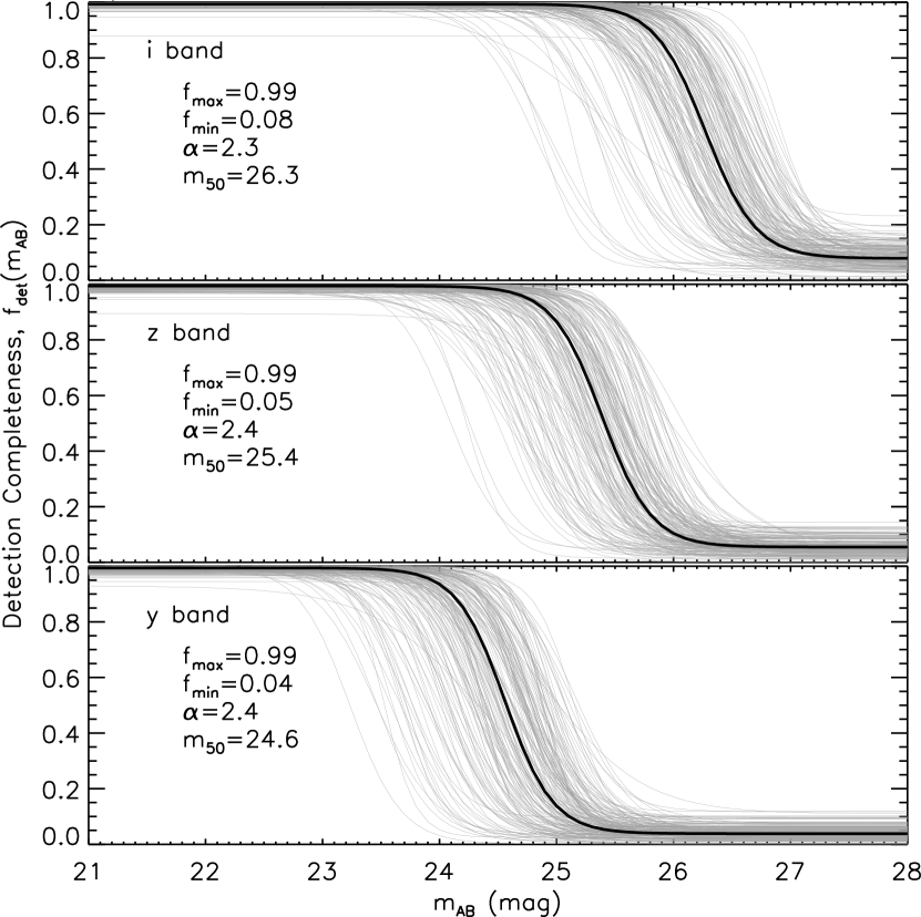
Figure 3: Detection completeness in the $i$ (top), $z$ (middle), and $y$ (bottom) bands as modeled by Equation 2, measured in each of the 180 random survey patches (thin gray lines). The thick solid lines represent the median completeness, calculated with the median parameter values as reported in each panel.

Figure 4: Comparison between $m_{\rm AB}^{5\sigma}$ (5$\sigma$ limiting magnitudes) and $m_{\rm AB}^{50}$ (50-% completeness magnitudes) in the $i$ (crosses), $z$ (dots), and $y$ (open circles) bands. The dotted line represents $m_{\rm AB}^{5\sigma}=m_{\rm AB}^{50}$.

Based on the above measurements and simulations, we quantified the detection completeness in the $z$ and $y$ bands over the entire survey area, as follows. For each 12′$\times$ 12′ patch (“$p$”), the completeness functions $f_{\rm det}(z_{\rm AB},p)$ and $f_{\rm det}(y_{\rm AB},p)$ were defined using Equation 2. We retrieved $z_{\rm AB}^{5\sigma}$ and $y_{\rm AB}^{5\sigma}$ from the survey database, and used them as surrogates for $z_{\rm AB}^{50}$ and $y_{\rm AB}^{50}$ in the individual patches. The parameters $f_{\rm max}$ and $f_{\rm min}$ were fixed to 1.0 and 0.0, respectively. Finally we assumed $\alpha$ = 2.4, the median value measured in both the $z$ and $y$ bands for the 180 patches in which we ran the simulations (the dispersion in this quantity measured by the median absolute deviation is $\Delta\alpha\sim 0.4$ in both bands). We checked that the present results are not sensitive to the choice of $\alpha$, since the detection completeness is close to 100 % at the present magnitude limit of $z_{\rm AB}<24.2$ mag.

3.2 Point Source Selection

The SHELLQs algorithm uses the criterion:

$$z_{\rm AB}-z_{\rm CModel,AB}<0.15$$ (3)

to identify point sources from the HSC database. The completeness of this selection was evaluated with a special HSC dataset on the COSMOS field, one of the two UltraDeep fields of the SSP survey, for which we have many more exposures than in a Wide field. This dataset was created by stacking a portion of the UltraDeep data taken during the best, median, or worst seeing conditions to match the Wide depth. We selected stars on this field with the Hubble Space Telescope (HST) Advanced Camera for Surveys (ACS) catalog (Leauthaud et al., 2007), and measured the fraction of stars meeting Equation 3. The results are presented in Figure 5. The completeness of our point source selection is close to 100 % at bright magnitudes, and decreases mildly to 90 % at $z_{\rm AB}\sim 24.0$ mag. No significant difference was observed between the different seeing conditions at $z_{\rm AB}<24$ mag. We fitted the above results for the median seeing with Equation 2, and obtained the best-fit parameters ($f_{\rm max}$, $f_{\rm min}$, $\alpha$, $z_{\rm AB}^{50}$) = (1.00, 0.72, 0.76, 24.5). This best-fit function, $f_{\rm ps}(z_{\rm AB})$, is used to simulate the selection completeness of point sources in the following.

Figure 5: Selection completeness of point sources, $f_{\rm ps}(z_{\rm AB})$, estimated with the HST ACS stars on the SSP Wide-depth dataset of the COSMOS field. The open circles, dots, and crosses represent the best, median, and worst seeing conditions, respectively. The best-fit function (Equation 2) to the median seeing data is represented by the dashed curve.

On the other hand, we found that the effect of resolved host galaxies on our quasar selection is negligible. This was simulated as follows. Since the luminosities of high-$z$ quasar host galaxies are unknown, we assumed the following, based on the low-$z$ results for SDSS quasars with similar nuclear luminosity to the SHELLQs quasars (Matsuoka et al., 2014, 2015): (i) the typical host galaxy luminosity ranges from $M_{UV}=-18$ to $-21$ mag (corresponding to $z_{\rm CModel,AB}\sim 25.5-28.5$ mag at $z=6$), and (ii) there is no correlation between the nuclear and host galaxy luminosities. The host galaxies were simulated with a sample of Lyman Break Galaxies (LBGs) at $z\sim 6$, found from the HSC-SSP Wide data (Harikane et al., 2018; Ono et al., 2018). We used 231 LBGs with $24.0<z_{\rm CModel,AB}<25.0$ mag, where AGN contamination to the sample is small (Ono et al., 2018). For each LBG, we randomly assigned $M_{UV}$ from $-18$ to $-21$ mag, assumed a flat UV spectral slope ($\beta=-2.0$; Stanway et al., 2005), and calculated the corresponding CModel flux ($f_{\rm CModel}^{\rm sim}$) at $z=6$. The PSF flux was calculated as $f_{\rm PSF}^{\rm sim}=f_{\rm CModel}^{\rm sim}\times(f_{\rm PSF}^{\rm obs}/f_{\rm CModel}^{\rm obs})$, where $f_{\rm PSF}^{\rm obs}/f_{\rm CModel}^{\rm obs}$ is the ratio between the PSF and CModel fluxes observed for the individual LBGs. Then we added various AGN fluxes ($f^{\rm AGN}=f_{\rm PSF}^{\rm AGN}=f_{\rm CModel}^{\rm AGN}$) artificially, and calculated the fraction of the simulated objects that satisfy Equation 3 and are thus “unresolved”:

$$-2.5\log\left(\frac{f_{\rm PSF}^{\rm sim}+f^{\rm AGN}}{f_{\rm CModel}^{\rm sim}+f^{\rm AGN}}\right)<0.15.$$ (4)

We found that the unresolved fraction is 100 % at AGN magnitudes $z_{\rm AB}<25.0$ mag, and decreases to 90 % at 26.0 mag. We thus conclude that our point source selection loses only a negligible fraction of quasars due to the resolved host galaxies, at the present magnitude limit of $z_{\rm AB}<24.2$ mag.

Here we note that compact galaxies could have $z_{\rm AB}-z_{\rm CModel,AB}<0.15$, and contaminate our quasar candidates. Indeed, so far we have discovered 25 high-$z$ galaxies in addition to 74 high-$z$ quasars from the HSC candidates. However, the present work uses only spectroscopically confirmed quasars, and thus is not affected by galaxy contamination.

3.3 Foreground flux contamination

As we wrote previously, we failed to recover one of the eight previously-known quasars in our survey footprint, due to $i$-band flux contamination of a foreground galaxy. The forced photometry can overestimate the $i$-band flux of an $i$-band dropout object superposed on a foreground source, because the aperture is defined by the object image in a redder band.

In order to simulate this effect, we randomly selected 10000 points from the HSC-SSP random source catalog in the way that we described in §2.3, and measured the $i$-band flux in an aperture placed at each point. The aperture size was set to twice the seeing FWHM at each position. The probability density distribution (PDF) of the measured fluxes is presented in Figure 6. The distribution around $f_{\nu}=0$ follows a Gaussian distribution, which represents the sky background fluctuation. In addition, the measured distribution has a tail toward higher $f_{\nu}$, which can be approximated by the function $f_{\rm fgd}(f_{\nu})\ =\ 3.3\ e^{-5\sqrt{f_{\nu,29}}}+0.0014$ ($f_{\nu,29}=f_{\nu}\times 10^{29}$ erg s^-1 cm^-2 Hz^-1) truncated at $f_{\nu,29}=5.8$ (corresponding to $i_{\rm AB}=22.0$ mag, above which the measured PDF contains less than 0.5 % of the total probability). This tail contains 12 % of the total probability, which is the fraction of sources affected by the foreground flux contamination. We use this function $f_{\rm fgd}(f_{\nu})$ in the following simulations.

The foreground flux contamination is much less significant in the $z$ and $y$ bands, in which high-$z$ quasars (meeting Equation 1) are clearly detected and the hscPipe deblender properly apportions the measured flux. Huang et al. (2018) demonstrated that the HSC flux measurement is accurate within 0.1 mag after deblending for the vast majority of the sources.

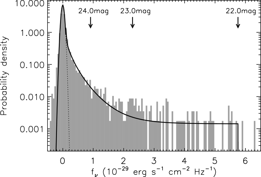
Figure 6: Probability density distribution of the $i$-band fluxes measured on random positions (histogram). The solid line represents the best-fit function, which is a combination of a Gaussian function (dotted line) and the function $f_{\rm fgd}(f_{\nu})$ defined in the text. The arrows mark the fluxes corresponding to $i_{\rm AB}=22.0$, 23.0, and 24.0 mag.

3.4 Total Completeness

The total completeness of our selection was estimated with quasar models, created from 319 SDSS spectra of luminous ($-27\leq M_{i}\leq-30$) quasars at $z\simeq 3$. This SDSS sample contains 29 radio-selected quasars, which are not sensitive to incompleteness in the color selection (see, e.g., Worseck & Prochaska, 2011). We selected a sample of 29 non-radio-selected quasars (i.e., objects selected for SDSS spectroscopy with other targeting criteria) from the remaining 290 objects, matched in luminosity to the radio-selected quasars, and compared the composite spectra of the two samples. This is shown in Figure 7. The composite spectra are almost identical to each other, indicating that the colors of radio- and color-selected quasars are similar, and that we introduce no significant bias by using the spectra of all 319 quasars in the simulations which follow. We note that the above radio-selected quasars are still a part of the magnitude-limited SDSS sample, and are biased against optically-faint populations such as obscured quasars. The present estimate does not include incompleteness due to such quasars that are missing from the SDSS spectroscopic sample.

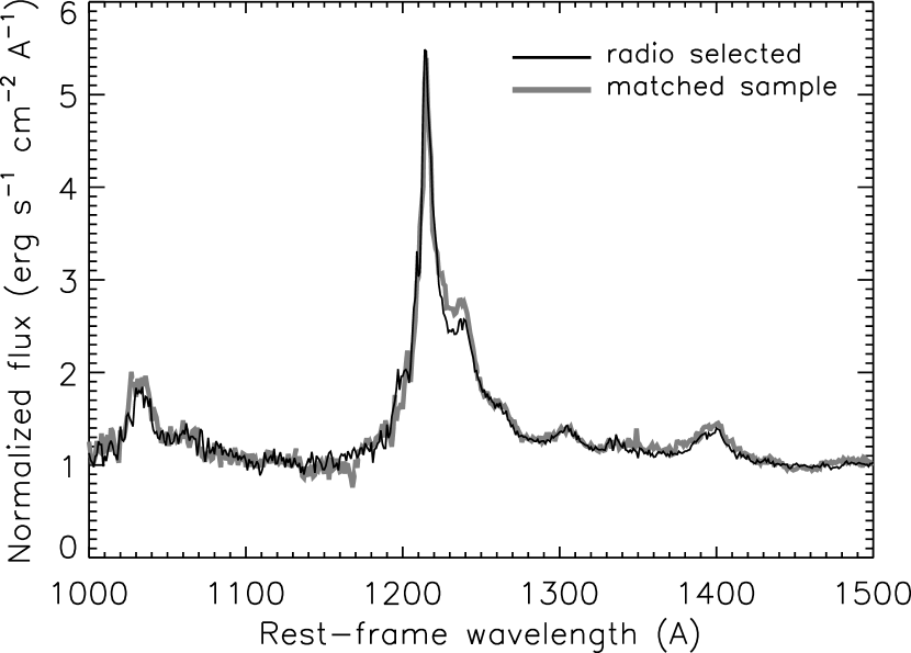
Figure 7: Composite spectra of 29 radio-selected SDSS quasars (black dashed line) and of a matched sample of 29 quasars selected by other criteria (gray solid line) at $z\simeq 3$. These composite spectra were created by converting the individual spectra to rest-frame wavelengths and normalizing the flux at 1450 Å, and then averaging all the input spectra.

Each of the above 319 spectra was redshifted to $z$ = 5.6 – 6.6, with $\Delta z=0.01$ steps, with appropriate correction for the different amounts of IGM H I absorption between $z\sim 3$ and $z\sim 6$. The IGM absorption in the original SDSS spectra was removed using the mean IGM effective optical depth ($\tau_{\rm eff}$) at $z\leq 3$ presented by Songaila (2004). We then added IGM absorption to the redshifted model spectra by assuming the mean and scatter of $\tau_{\rm eff}$ taken from Eilers et al. (2018). The absorption started at a wavelength corresponding to 1 proper Mpc from the quasar, to model the effect of quasar proximity zones. The assumed proximity radius is appropriate for the mean luminosity of the SHELLQs quasars ($M_{1450}\sim-23$ mag; Eilers et al., 2017). The damping wing of the IGM absorption was modeled following the prescription in Totani et al. (2006).

At this stage we found that the mean and the scatter of rest-frame Ly$\alpha$ equivalent widths (EWs) of the model quasars were 64 $\pm$ 16 Å (this includes the effect of IGM absorption, and was measured with a subset of model quasars matched in redshift to the observed sample; the scatter was measured with the median absolute deviation), which are larger than those of the observed sample, 38 $\pm$ 12 Å. This trend is opposite to the luminosity dependence known as the Baldwin effect, and may be in part due to the redshift dependence of quasar SEDs, including a higher fraction of weak-line quasars found at higher redshifts (e.g., Bañados et al., 2016; Shen et al., 2018). We scaled the Ly$\alpha$ line of the model spectra, with the scaling factor chosen randomly from a Gaussian distribution of mean 0.6 and standard deviation 0.2, which roughly reproduces the observed EW distribution. Since the HSC bands cover only a limited portion (rest-frame wavelength $\lesssim 1500$ Å) of the high-$z$ quasar spectra redward of Ly$\alpha$, differences in other emission lines or continuum slopes between the $z\sim 3$ SDSS quasars and the SHELLQs quasars would not be very relevant here.

The simulations of our quasar selection were performed with five million points selected from the HSC-SSP random source catalog, using the pixel flag conditions in Equation 1. We randomly assigned one of the above quasar models to each random point, and calculated apparent magnitudes, assuming an absolute magnitude drawn from a uniform distribution from $M_{1450}=-20$ to $-28$ mag. We then added simulated errors to the apparent magnitudes, assuming a Gaussian error distribution with standard deviation ($\sigma$) equal to the sky background RMS, computed from the $5\sigma$ limiting magnitudes of the corresponding patches ($m^{5\sigma}_{\rm AB}$; see above). We simulated the foreground flux contamination using the PDF $f_{\rm fgd}(f_{\nu})$, derived in §3.3.

We then applied additional flux scatter with a Gaussian distribution with standard deviation 0.3 mag, in each of the three bands. This was necessary to match the color distributions of the model and observed quasars, while it does not change the derived LF significantly. This additional scatter may account for other sources of flux fluctuation than explicitly considered above, including photometry errors due to cosmic rays, image artifacts, and imperfect source deblending, the host galaxy contribution, and difference in the intrinsic SED shapes between the above SDSS quasars and the SHELLQs quasars (see, e.g., Niida et al., 2016). The resultant color distributions of the model and observed quasars are presented in Figure 8.

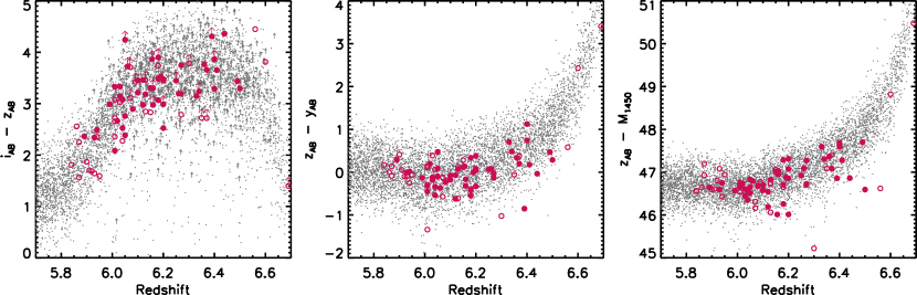
Figure 8: The $i_{\rm AB}-z_{\rm AB}$ (left), $z_{\rm AB}-y_{\rm AB}$ (middle), and $z_{\rm AB}-M_{1450}$ (right) distributions of the simulated quasars with $z_{\rm AB}<24.2$ mag (gray dots). The arrows represent 2$\sigma$ lower limits. The SHELLQs quasars included in and excluded from the present complete sample are represented by the filled and open circles, respectively.

We selected a portion of the above simulated quasars, such that a quasar with simulated magnitudes ($z_{\rm AB}$, $y_{\rm AB}$) on a patch $p$ has a probability $f_{\rm det}(z_{\rm AB},p)\times f_{\rm det}(y_{\rm AB},p)\times f_{\rm ps}(z_{\rm AB})$ of being selected. This accounts for the field variance of the detection completeness. We further selected those meeting the following conditions:

$$z_{\rm AB}<z_{\rm AB}^{\rm slim}\ \&\ \sigma_{z}<0.155\ \&\ i_{\rm AB}-z_{\rm AB}>2.0.$$ (5)

Finally we calculated Bayesian quasar probabilities ($P_{\rm Q}^{\rm B}$) for the selected sources, using the method described in Matsuoka et al. (2016), and counted the number of sources with $P_{\rm Q}^{\rm B}>0.1$. The total completeness, $f_{\rm comp}(z,M_{1450})$, is given by the ratio between the output and input numbers of random sources, calculated in bins of $z$ and $M_{1450}$. There are roughly 400 simulated quasars in each bin with sizes $\Delta{z}=0.01$ and $\Delta{M_{1450}}=0.05$.

Figure 9 presents the total completeness derived above. The selection of the present complete sample is most sensitive to $5.9<z<6.5$ and $M_{1450}<-22.5$ mag. The completeness drops at $z\leq 5.9$ due to the color cut of $i-z>2.0$, while it drops more gradually at $z\geq 6.5$ due to the increasing contamination of brown dwarfs (which reduces the quasar probability $P_{\rm Q}^{\rm B}$). The figure also shows that several quasars located in the high completeness region are not included in the complete sample. This is caused by various reasons; some quasars are in survey fields that fail to meet the pixel flag conditions (Equation 1) in the S17A data release, and some quasars have $i-z$ colors just below the threshold of 2.0. The faintest quasars with $M_{1450}>-22.5$ mag simply fail to meet the condition $z_{\rm AB}<z_{\rm AB}^{\rm slim}$.

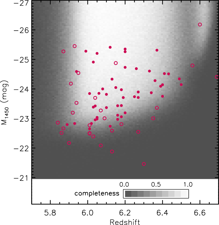
Figure 9: Total completeness of the SHELLQs complete quasar selection, ranging from $f_{\rm comp}(z,M_{1450})=1.0$ in white to 0.0 in gray. The SHELLQs quasars included in and excluded from the present complete sample are marked by the filled and open circles, respectively.

In the following section, we use the completeness functions of the SDSS, CFHQS, and SHELLQs to derive a single LF. These functions were all derived with quasar models tied to spectra of SDSS quasars at $z\sim 3$, while the IGM absorption models in the SDSS and CFHQS were created from older $\tau_{\rm eff}$ data than those we used here for the SHELLQs sample. We tested another IGM absorption model for the SHELLQs sample, with the mean and scatter of the $\tau_{\rm eff}$ determined empirically to reproduce the data in Songaila (2004), and found little change in the derived completeness or LF. In addition, while the completeness correction is most important at the faintest luminosity of a given sample, the faintest SDSS/CFHQS quasars have smaller available volumes ($V_{\rm a}$; see below and Table 2) and thus smaller weights in LF calculation than do the CFHQS/SHELLQs quasars with similar luminosities and high completeness. Thus we conclude that no significant bias is introduced by combining the completeness functions of the three surveys.

4 Luminosity Function

First, we derive the binned LF using the 1/$V_{\rm a}$ method (Avni & Bahcall, 1980). The cosmic volume available to discover a quasar, in a magnitude bin $\Delta M_{1450}$, is given by

$$V_{\rm a}=\frac{1}{\Delta M_{1450}}\int_{\Delta M_{1450}}\int_{\Delta z}f_{\rm comp}(z,M_{1450})\ \frac{dV_{\rm c}}{dz}\ dz\ dM_{1450},$$ (6)

where $\Delta z$ represents the redshift range to calculate the LF, and $dV_{\rm c}/dz$ is the co-moving volume element probed by a survey. The binned LF and its uncertainty are then given by

$$\Phi_{\rm b}(M_{1450})=\frac{1}{\Delta M_{1450}}\sum\frac{1}{V_{\rm a}},$$

$$\Delta\Phi_{\rm b}(M_{1450})=\frac{1}{\Delta M_{1450}}\left[\sum\left(\frac{1}{V_{\rm a}}\right)^{2}\right]^{1/2},$$ (7)

where the sum is taken over the quasars in the magnitude bin. This expression ignores the redshift evolution of the LF over the measured range ($5.7\leq z\leq 6.5)$; we will take this evolution into account in the parametric LF described below. Here we combine the three complete samples of quasars from the SDSS, the CFHQS, and the SHELLQs, to derive a single binned LF over $-22<M_{1450}<-30$ mag (we use the completeness functions and the survey areas of the SDSS and CFHQS described in §2.1 and §2.2). We set the bin size $\Delta M_{1450}=0.5$ mag, except at both ends of the luminosity coverage where the sample size is small. The results of this calculation are listed in Table 4 and presented in Figure 10.

The derived LF agrees well with the previous results from the SDSS (Jiang et al., 2016) and the CFHQS (Willott et al., 2010) at $M_{1450}<-25$ mag, and significantly improves the accuracy at fainter magnitudes. It may be worth mentioning that the number density of the brightest bin measured by Jiang et al. (2016) and in this work do not exactly match, although the two works use a single SDSS quasar in common. This is due to the different choice of the bin center and width, which is known to have a significant impact on the binned LF when the sample size is small. On the other hand, we significantly increased the available survey volume for the faintest bin at $M_{1450}=-22.00$, and found a number density lower than (but consistent within 1$\sigma$) the previous measurement by Willott et al. (2010).

Table 4: Binned luminosity function

$M_{1450}$	$\Delta M_{1450}$	$\Phi_{\rm b}(M_{1450})$	$N_{\rm obj}$
		(Gpc-3 mag-1)
$-22.00$	1.0	16.2 $\pm$ 16.2	1
$-22.75$	0.5	23.0 $\pm$ 8.1	8
$-23.25$	0.5	10.9 $\pm$ 3.6	9
$-23.75$	0.5	8.3 $\pm$ 2.6	10
$-24.25$	0.5	6.6 $\pm$ 2.0	11
$-24.75$	0.5	7.0 $\pm$ 1.7	17
$-25.25$	0.5	4.6 $\pm$ 1.2	14
$-25.75$	0.5	1.33 $\pm$ 0.60	5
$-26.25$	0.5	0.90 $\pm$ 0.32	8
$-26.75$	0.5	0.58 $\pm$ 0.17	12
$-27.50$	1.0	0.242 $\pm$ 0.061	16
$-29.00$	2.0	0.0079 $\pm$ 0.0079	1
$-22.75$	0.5	14.4 $\pm$ 6.4	5
$-23.25$	0.5	8.5 $\pm$ 3.2	7

Note. — $M_{1450}$ and $\Delta M_{1450}$ represent the center and width of each magnitude bin, respectively. $N_{\rm obj}$ represents the number of quasars contained in the bin. The last two rows report the LF at $-22.5<M_{1450}<-23.5$ excluding narrow Ly$\alpha$ quasars (see the text).

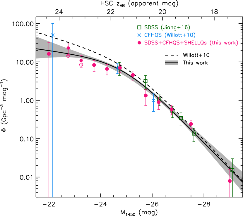
Figure 10: Binned LF measured by the SDSS (squares; Jiang et al., 2016), the CFHQS (crosses; Willott et al., 2010), and this work combining the SDSS, CFHQS, and SHELLQs samples (dots). The open circles show the LF excluding the five quasars with narrow Ly$\alpha$ (see the text). The solid line represents our parametric LF with the 1$\sigma$ confidence interval shown by the shaded area, while the dashed line represents the parametric LF of Willott et al. (2010). All the parametric LFs are calculated at $z=6.0$.

Next, we derive the parametric LF, using a commonly-used double power-law function:

$$\Phi_{\rm p}(M_{1450})=\frac{10^{k(z-6)}\Phi^{*}}{10^{0.4(\alpha+1)(M_{1450}-M_{1450}^{*})}+10^{0.4(\beta+1)(M_{1450}-M_{1450}^{*})}},$$ (8)

where $\alpha$ and $\beta$ are the faint- and bright-end slopes, respectively. We fix the redshift evolution term to $k=-0.47$ (Willott et al., 2010) or $k=-0.7$ (Jiang et al., 2016); we found that the choice makes little difference in the determination of other parameters (see below). Following the argument in Jiang et al. (2016), we adopt $k=-0.7$ as our standard value. The parameters $M_{1450}^{*}$ and $\Phi^{*}$ give the break magnitude and normalization of the LF, respectively.

We perform a maximum likelihood fit (Marshall et al., 1983) to determine the four free parameters ($\alpha$, $\beta$, $M_{1450}^{*}$, and $\Phi^{*}$). Specifically, we maximize the likelihood $L$ by minimizing $S=-2\ln{L}$, given by

$$S=-2\sum\ln\left[\Phi_{\rm p}(z,M_{1450})\ f_{\rm comp}(z,M_{1450})\right]$$

$$+2\int_{-\infty}^{+\infty}\int_{-\infty}^{+\infty}\Phi_{\rm p}(M_{1450},z)\ f_{\rm comp}(z,M_{1450})\ \frac{dV_{\rm c}}{dz}\ dz\ dM_{1450},$$

where the sum in the first term is taken over all quasars in the sample. The resultant parametric LF is presented in Figure 10, and the best-fit LF parameters are listed in the first row of Table 5. Figure 11 presents the confidence regions of the individual LF parameters.

Table 5: Parametric luminosity function

	$\Phi^{*}$	$M^{*}_{1450}$	$\alpha$	$\beta$	$k$
	(Gpc-3 mag-1)
Standard	$10.9^{+10.0}_{-6.8}$	$-24.90^{+0.75}_{-0.90}$	$-1.23^{+0.44}_{-0.34}$	$-2.73^{+0.23}_{-0.31}$	$-0.7$
Different $k$	$9.5^{+9.6}_{-6.2}$	$-25.02^{+0.82}_{-0.98}$	$-1.27^{+0.42}_{-0.33}$	$-2.74^{+0.24}_{-0.33}$	$-0.47$
Free $k$	$7.8^{+9.2}_{-5.6}$	$-25.18^{+0.88}_{-1.13}$	$-1.34^{+0.43}_{-0.34}$	$-2.76^{+0.26}_{-0.40}$	$-0.2^{+0.2}_{-0.1}$
Narrow-Ly$\alpha$ quasars excluded	$14.1^{+6.8}_{-6.7}$	$-24.64^{+0.54}_{-0.66}$	$-0.88^{+0.48}_{-0.39}$	$-2.67^{+0.18}_{-0.25}$	$-0.7$
Quasars with $z>5.9$	$8.1^{+12.3}_{-5.9}$	$-25.30^{+1.05}_{-1.15}$	$-1.39^{+0.45}_{-0.32}$	$-2.79^{+0.32}_{-0.48}$	$-0.7$

This is the first time that observed data have shown a clear break in the LF for $z\sim 6$ quasars. The bright-end slope, $\beta=-2.73^{+0.23}_{-0.31}$, agrees very well with those reported previously by Willott et al. (2010, $\beta=-2.81$, with the faint-end slope fixed to $\alpha=-1.5$) and Jiang et al. (2016, $\beta=-2.8\pm 0.2$, fitting only the brightest portion of the LF). The break magnitude is $M_{1450}^{*}=-24.90^{+0.75}_{-0.90}$, and the LF flattens significantly toward lower luminosities. The slope $\alpha=-1.23^{+0.44}_{-0.34}$ is even consistent with a completely flat faint-end LF (i.e., $\alpha=1.0$).

We also performed LF calculations with $k$ fixed to $-0.47$ or allowed to vary as a free parameter, and found that the other LF parameters are not very sensitive to the choice of $k$. These results are listed in the second and third rows of Table 5. The fitting with variable $k$ favors relatively flat LF evolution ($k=-0.2^{+0.2}_{-0.1}$), which may be consistent with a tendency that $k$ is smaller for lower-luminosity quasars seen in Jiang et al. (2016, their Figure 10). But given the short redshift baseline of the present sample, we chose to adopt the fixed value $k=-0.7$ for our standard LF.

Recently, Kulkarni et al. (2018) reported a very bright break magnitude of $M_{1450}^{*}=-29.2^{+1.1}_{-1.9}$ mag at $z\sim 6$, by re-analyzing the quasar sample constructed by Jiang et al. (2016), Willott et al. (2010), and Kashikawa et al. (2015). However, their data favor a single power-law LF, and thus the break magnitude was forced to be at the bright end of the sample in their LF fitting (Kulkarni et al., 2018). The present work indicates that the LF breaks at a much fainter magnitude, in the luminosity range that has been poorly explored previously.

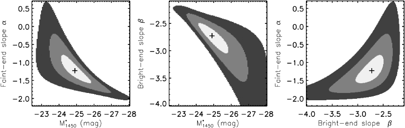
Figure 11: Confidence regions (light gray: 1$\sigma$, gray: 2$\sigma$, dark gray: 3$\sigma$) of the individual LF parameters. The best-fit values are marked by the crosses.

It may be worth noting that the CFHQS-deep survey discovered one quasar in the $M_{1450}=-22.00$ bin from $V_{\rm a}=0.003$ Gpc³, while SHELLQs discovered no quasars (in the present complete sample) in the same $M_{1450}$ bin from $V_{\rm a}=0.058$ Gpc³ (Table 2). This is presumably due to statistical fluctuations. Based on the present parametric LF, the expected total number of quasars in the CFHQS-deep survey is roughly one, with the most likely luminosity in the range $-25\lesssim M_{1450}\lesssim-22$ mag. In reality the survey discovered one quasar with $M_{1450}=-21.5$ mag and none at brighter magnitudes, which is consistent with the expectation. On the other hand, the expected number of SHELLQs quasars in the $M_{1450}=-22.00$ bin is roughly one. This is consistent with the actual discovery of no quasars in this bin, given Poisson noise.

The SHELLQs complete sample used here includes five objects with narrow Ly$\alpha$ lines (FWHM $<500$ km s^-1) at $-23.5<M_{1450}<-22.5$. We classified them as quasars based on their extremely high Ly$\alpha$ luminosities, featureless continuum, and possible mini broad absorption line system of N V $\lambda$1240 seen in their composite spectrum (Matsuoka et al., 2018a). It is possible that they are not in fact type-1 quasars, so for reference, we re-calculated the binned LF at $-23.5<M_{1450}<-22.5$ omitting these five objects, and listed the results in the last two rows of Table 4. The parametric LF in this case is reported in the fourth row of Table 5, which shows a modest difference from the standard case.

We also calculated the LF by limiting the sample to the 89 quasars in our complete sample at $z>5.9$, the redshift range over which the CFHQS and SHELLQs are most sensitive (see Figure 1). The resultant parametric LF is listed in the last row of Table 5. The LF in this case has slightly brighter $M^{*}_{1450}$ and steeper $\alpha$ than the standard LF, but the difference is smaller than the fitting uncertainty.

Figure 12 displays our LF and several past measurements below the break magnitude, $M_{1450}\geq-25$ mag. We found a flatter LF than reported in Willott et al. (2010) and Onoue et al. (2017, and their previous paper ()), who had only a few low-luminosity quasars in their samples. The extrapolation of our LF underpredicts the number densities of faint AGNs compared to those reported by Giallongo et al. (2015), while the former is consistent with the more recent measurements by Parsa et al. (2018). On the other hand, we note that the above X-ray measurements are immune to dust obscuration, and that the discrepancy with the rest-UV measurements, if any, could be due to the presence of a large population of obscured AGNs in the high-$z$ universe. Finally, Figure 12 indicates that LBGs (taken from Ono et al., 2018) outnumber quasars at $M_{1450}>-23$ mag. This is consistent with our experience from the SHELLQs survey, which found increasing numbers of LBGs contaminating the quasar candidate sample at $z_{\rm AB}>23$ mag (Matsuoka et al., 2016, 2018a, 2018b).

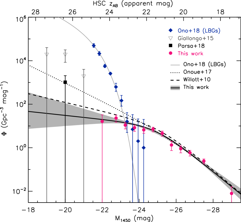
Figure 12: Binned LFs measured by Ono et al. (2018, for LBGs; diamonds), Giallongo et al. (2015, triangles), Parsa et al. (2018, squares), and this work (dots). In the X-ray measurements by Giallongo et al. (2015) and Parsa et al. (2018), the rest-UV magnitudes $M_{1450}$ were estimated from the optical photometry of the galaxies matched to the X-ray sources. The lines represent the parametric LFs measured by Ono et al. (2018, for LBGs; gray solid), Onoue et al. (2017, their case $1^{\prime}$; dotted), Willott et al. (2010, dashed), and this work (solid; the 1$\sigma$ confidence interval is shown by the shaded area). All the parametric LFs are calculated at $z=6.0$.

We compare the present LF with those recently derived at $z\sim 4$ (Akiyama et al., 2018) and $z\sim 5$ (McGreer et al., 2018) in Figure 13. The overall shape of the binned LF remains relatively similar, while there is a steep decline of the total number density toward higher redshifts. However, the best-fit break magnitudes reported in the above studies differ substantially, i.e., $M_{1450}^{*}$ = ($-25.36\pm 0.13$, $-27.42^{+0.22}_{-0.26}$, $-24.90^{+0.75}_{-0.90}$) at $z\sim$ (4, 5, 6). This may be in part due to the choice of the fixed bright-end slope $\beta=-4.0$ in McGreer et al. (2018), which is significantly steeper than measured at $z\sim 4$ ($\beta\sim-3.1$; Akiyama et al., 2018) or at $z\sim 6$ ($\beta\sim-2.7$; this work). As shown in the middle panel of Figure 11, the bright-end slope and the break magnitude are strongly covariant in the parametric LF fitting. We found that the binned LF of McGreer et al. (2018) can also be fitted reasonably well with $\beta=-3.0$, as shown in Figure 13 (dashed line). The best-fit break magnitude in this case is $M_{1450}^{*}=-25.6\pm 0.3$, which is close to the break magnitudes at $z\sim 4$ and $z\sim 6$. The figure also displays the parametric LFs reported by Kulkarni et al. (2018); while these LFs match the data in the luminosity ranges covered by their sample, the LFs seem to overpredict the number densities of fainter quasars presented in the recent studies by Akiyama et al. (2018), McGreer et al. (2018), and this paper.

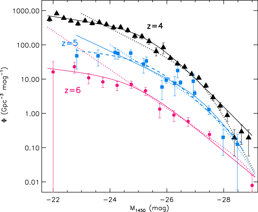
Figure 13: Binned LFs at $z\sim 4$ (triangles; Akiyama et al., 2018), $z\sim 5$ (squares; McGreer et al., 2018), and $z\sim 6$ (dots; this work), along with the parametric LFs at those redshifts (the three solid lines). The dashed line represents the parametric LF fitted to the McGreer et al. (2018) data with the fixed bright-end slope $\beta=-3.0$ (see the text), while the three dotted lines represent the parametric LFs at the three redshifts reported by Kulkarni et al. (2018).

Since the LF is a product of the mass function and the Eddington ratio function of SMBHs, it is not straightforward to interpret the significant flattening observed at $M_{1450}\geq-25$ mag, in terms of a unique physical model. It could indicate relatively mass-independent number densities and/or quasar radiation efficiency, at low SMBH masses. We will compare our LF with theoretical models in a forthcoming paper. Alternatively, as discussed above, the LF flattening may indicate an increasing fraction of obscured AGNs toward low luminosities, especially in light of the X-ray results in Figure 12. This could be an interesting subject for future deep X-ray observations, such as those that ATHENA (Nandra et al., 2013) will achieve.

5 Contribution to Cosmic Reionization

There is much debate about the source of photons that are responsible for cosmic reionization, as we discussed in §1. Here we derive the total ionizing photon density from quasars per unit time, $\dot{n}_{\rm ion}$ (s^-1 Mpc^-3), and compare with that necessary to keep the IGM fully ionized. The ionizing photon density can be calculated as:

$$\dot{n}_{\rm ion}=f_{\rm esc}\ \epsilon_{1450}\ \xi_{\rm ion},$$ (10)

where $f_{\rm esc}$ is the photon escape fraction, $\epsilon_{1450}$ (erg s^-1 Hz^-1 Mpc^-3) is the total photon energy density from quasars at 1450 Å:

$$\epsilon_{1450}=\int\Phi_{\rm p}(M_{1450},z)L_{1450}dM_{1450},$$ (11)

and $\xi_{\rm ion}$ [s^-1/(erg s^-1 Hz^-1)] is the number of ionizing photons from a quasar with a monochromatic luminosity $L_{1450}$ = 1 erg s^-1 Hz^-1 at 1450 Å:

$$\xi_{\rm ion}=(L_{1450})^{-1}\int^{4\nu_{\rm LL}}_{\nu_{\rm LL}}\frac{L_{\nu}}{h\nu}d\nu.$$ (12)

Equation 11 was integrated from $M_{1450}=-18$ to $-30$ mag, using the parametric LF derived in the previous section. In Equation 12, we used a broken power-law quasar SED ($f_{\nu}\propto\nu^{-1.70}$ at $\lambda<912\$Å and $\propto\nu^{-0.61}$ at $\lambda>912\$Å) presented by Lusso et al. (2015), and integrated from the H I Lyman limit (frequency $\nu=\nu_{\rm LL}$) to the He II Lyman limit ($\nu=4\nu_{\rm LL}$). The implicit assumptions here are that the above SED, created from luminous quasars at $z\sim 2.4$, holds for the present high-$z$ quasars, and that all the ionizing photons with $\nu<4\nu_{\rm LL}$ are absorbed by the IGM. The resultant photon density is $\dot{n}_{\rm ion}=10^{48.8\pm 0.1}$ s^-1 Mpc^-3 at $z=6.0$ for $f_{\rm esc}=1$. We would get lower $\dot{n}_{\rm ion}$ for $f_{\rm esc}<1$, which may be the case for low-luminosity quasars (Cristiani et al., 2016; Micheva et al., 2017; Grazian et al., 2018). The energy density at 912 Å is estimated to be $\epsilon_{912}=10^{22.9\pm 0.1}$ erg s^-1 Hz^-1 Mpc^-3, which is close to the value reported by Haardt & Madau (2012) at $z=6$. The results presented in this section change very little when the faint limit of the integral in Equation 11 is changed to $M_{1450}=-10$ mag, or when the five SHELLQs quasars with narrow Ly $\alpha$ (see §4) are excluded.

On the other hand, the evolution of the H II volume-filling factor in the IGM, $Q_{\rm HII}(t)$, is given by

$$\frac{dQ_{\rm HII}}{dt}=\frac{\dot{n}_{\rm ion}}{\bar{n}_{\rm H}}-\frac{Q_{\rm HII}}{\bar{t}_{\rm rec}},$$ (13)

where $\bar{n}_{\rm H}$ and $\bar{t}_{\rm rec}$ are the mean hydrogen density and recombination time, respectively (Madau et al., 1999). In the ionized IGM with $Q_{\rm HII}=1.0$, the rate of ionizing photon density which balances recombination is given by

$$\dot{n}^{\rm crit}_{\rm ion}=\frac{\bar{n}_{\rm H}}{\bar{t}_{\rm rec}}=10^{50.0}C_{\rm HII}\left(\frac{1+z}{7}\right)^{3}({\rm s}^{-1}{\rm Mpc}^{-3}),$$ (14)

where $C_{\rm HII}$ represents an effective H II clumping factor (Bolton & Haehnelt, 2007). The ionizing photon density we found above, given our LF, is less than 10 % of $\dot{n}^{\rm crit}_{\rm ion}$ for the plausible range of $C_{\rm HII}=1.0-5.0$ (Shull et al., 2012). This means that quasars alone cannot sustain reionization. For reference, we would get $\dot{n}_{\rm ion}=10^{50.3}$ s^-1 Mpc^-3 $\sim\dot{n}^{\rm crit}_{\rm ion}$ if we assumed no LF break ($\alpha=\beta=-2.73$) and integrated Equation 11 from $M_{1450}=-18$ to $-30$ mag.

Finally, we numerically integrate Equation 13 and track the evolution of $Q_{\rm HII}$ driven solely by quasar radiation. We assume that the IGM was neutral at $z=15$, and that $\dot{n}_{\rm ion}$ was constant in time (i.e., it stayed at $10^{48.8\pm 0.1}$ s^-1 Mpc^-3) or evolved as $\propto 10^{-0.7z}$ (i.e., proportional to the LF normalization found around $z=6$) at $5<z<15$. We followed Robertson et al. (2015) to estimate $\bar{n}_{\rm H}$ and $\bar{t}_{\rm rec}$. The results of this calculation are presented in Figure 14. For reference, we also plot the $Q_{\rm HII}$ evolution driven by star-forming galaxies, using the star formation rate density at $z<15$ presented in Robertson et al. (2015). This figure demonstrates that star-forming galaxies can supply enough high-energy photons to ionize the IGM by $z=6$, while quasars cannot. We thus conclude that quasars are not a major contributor to reionization. Even if there is a large population of obscured AGNs that are missed by rest-UV surveys (see the discussion in §4), they are unlikely to release many ionizing photons, since the ionizing photon escape fraction from these objects would be close to $f_{\rm esc}\sim 0$.

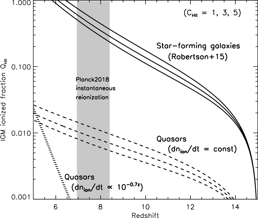
Figure 14: Evolution of the H II volume-filling factor in the IGM. The three solid curves represent contribution from star-forming galaxies (Robertson et al., 2015) for the clumping factor $C_{\rm HII}$ = 1, 3, 5 from top to bottom. The dashed and dotted curves represent the quasar contribution for the same $C_{\rm HII}$ values, for models with constant $\dot{n}_{\rm ion}$ or $\dot{n}_{\rm ion}\propto 10^{-0.7z}$, respectively (see the text). The shaded area represents the 1$\sigma$ confidence interval of the instantaneous reionization redshift, taken from the Planck measurements (Planck Collaboration et al., 2018).

6 Summary

This paper presented new measurements of the quasar LF at $z\sim 6$, which is now established over an unprecedentedly wide magnitude range from $M_{1450}=-30$ to $-22$ mag. We collected a complete sample of 110 quasars from the SDSS, the CFHQS, and the SHELLQs surveys. The completeness of the SHELLQs quasar selection was carefully evaluated, and we showed that the selection is most sensitive to quasars with $5.9<z<6.5$ and $M_{1450}<-22.5$ mag. The resultant binned LF is consistent with previous results at $M_{1450}<-25$ mag, while it exhibits significant flattening at fainter magnitudes. The maximum likelihood fit of a double power-law function to the sample yielded a faint-end slope $\alpha=-1.23^{+0.44}_{-0.34}$, a bright-end slope $\beta=-2.73^{+0.23}_{-0.31}$, a break magnitude $M_{1450}^{*}=-24.90^{+0.75}_{-0.90}$, and a characteristic space density $\Phi^{*}=10.9^{+10.0}_{-6.8}$ Gpc^-3 mag^-1. The rate of ionizing photon density from quasars is $\dot{n}_{\rm ion}=10^{48.8\pm 0.1}$ s^-1 Mpc^-3, when integrated over $-18<M_{1450}<-30$ mag. This accounts for $<$10 % of the critical rate necessary to keep the IGM fully ionized at $z=6.0$. We conclude that quasars are not a major contributor to cosmic reionization.

The HSC-SSP survey is making steady progress toward its goal of observing 1,400 deg² in the Wide layer. We will continue follow-up spectroscopy to construct a larger complete sample of $z\sim 6$ quasars, down to lower luminosity than probed in the present work. We are also starting an intensive effort to explore higher redshifts, with the aim of establishing the quasar LF at $z\sim 7$. At the same time, we are collecting near-IR spectra to measure the SMBH masses and mass accretion rates, which will be used in combination with the LFs to understand the growth of SMBHs in the early Universe. The ALMA follow-up observations are also ongoing, which will provide valuable information on the formation and evolution of the host galaxies.

References

- Abazajian et al. (2004) Abazajian, K., Adelman-McCarthy, J. K., Agüeros, M. A., et al. 2004, AJ, 128, 502
- Aihara et al. (2018a) Aihara, H., Armstrong, R., Bickerton, S., et al. 2018, PASJ, 70, S8
- Aihara et al. (2018b) Aihara, H., Arimoto, N., Armstrong, R., et al. 2018, PASJ, 70, S4
- Akiyama et al. (2018) Akiyama, M., He, W., Ikeda, H., et al. 2018, PASJ, 70, S34
- Annis et al. (2014) Annis, J., Soares-Santos, M., Strauss, M. A., et al. 2014, ApJ, 794, 120
- Avni & Bahcall (1980) Avni, Y., & Bahcall, J. N. 1980, ApJ, 235, 694
- Bañados et al. (2016) Bañados, E., Venemans, B. P., Decarli, R., et al. 2016, ApJS, 227, 11
- Bañados et al. (2018) Bañados, E., Venemans, B. P., Mazzucchelli, C., et al. 2018, Nature, 553, 473
- Bertin & Arnouts (1996) Bertin, E., & Arnouts, S. 1996, A&AS, 117, 393
- Bolton & Haehnelt (2007) Bolton, J. S., & Haehnelt, M. G. 2007, MNRAS, 382, 325
- Bosch et al. (2018) Bosch, J., Armstrong, R., Bickerton, S., et al. 2018, PASJ, 70, S5
- Bouwens et al. (2011) Bouwens, R. J., Illingworth, G. D., Labbe, I., et al. 2011, Nature, 469, 504
- Bouwens et al. (2015) Bouwens, R. J., Illingworth, G. D., Oesch, P. A., et al. 2015, ApJ, 803, 34
- Cappelluti et al. (2016) Cappelluti, N., Comastri, A., Fontana, A., et al. 2016, ApJ, 823, 95
- Chambers et al. (2016) Chambers, K. C., Magnier, E. A., Metcalfe, N., et al. 2016, arXiv:1612.05560
- Coupon et al. (2018) Coupon, J., Czakon, N., Bosch, J., et al. 2018, PASJ, 70, S7
- Cristiani et al. (2016) Cristiani, S., Serrano, L. M., Fontanot, F., Vanzella, E., & Monaco, P. 2016, MNRAS, 462, 2478
- D’Aloisio et al. (2017) D’Aloisio, A., Upton Sanderbeck, P. R., McQuinn, M., Trac, H., & Shapiro, P. R. 2017, MNRAS, 468, 4691
- Edge et al. (2013) Edge, A., Sutherland, W., Kuijken, K., et al. 2013, The Messenger, 154, 32
- Eilers et al. (2018) Eilers, A.-C., Davies, F. B., & Hennawi, J. F. 2018, ApJ, 864, 53
- Eilers et al. (2017) Eilers, A.-C., Davies, F. B., Hennawi, J. F., et al. 2017, ApJ, 840, 24
- Fan et al. (2006) Fan, X., Strauss, M. A., Becker, R. H., et al. 2006, AJ, 132, 117
- Fukugita et al. (1996) Fukugita, M., Ichikawa, T., Gunn, J. E., et al. 1996, AJ, 111, 1748
- Giallongo et al. (2015) Giallongo, E., Grazian, A., Fiore, F., et al. 2015, A&A, 578, A83
- Giavalisco et al. (2004) Giavalisco, M., Ferguson, H. C., Koekemoer, A. M., et al. 2004, ApJ, 600, L93
- Glikman et al. (2011) Glikman, E., Djorgovski, S. G., Stern, D., et al. 2011, ApJ, 728, L26
- Grazian et al. (2018) Grazian, A., Giallongo, E., Boutsia, K., et al. 2018, A&A, 613, A44
- Haardt & Madau (2012) Haardt, F., & Madau, P. 2012, ApJ, 746, 125
- Harikane et al. (2018) Harikane, Y., Ouchi, M., Ono, Y., et al. 2018, PASJ, 70, S11
- Huang et al. (2018) Huang, S., Leauthaud, A., Murata, R., et al. 2018, PASJ, 70, S6
- Ikeda et al. (2012) Ikeda, H., Nagao, T., Matsuoka, K., et al. 2012, ApJ, 756, 160
- Ikeda et al. (2011) Ikeda, H., Nagao, T., Matsuoka, K., et al. 2011, ApJ, 728, L25
- Ishigaki et al. (2018) Ishigaki, M., Kawamata, R., Ouchi, M., et al. 2018, ApJ, 854, 73
- Izumi et al. (2018) Izumi, T., Onoue, M., Shirakata, H., et al. 2018, arXiv:1802.05742 (Paper III)
- Jiang et al. (2014) Jiang, L., Fan, X., Bian, F., et al. 2014, ApJS, 213, 12
- Jiang et al. (2016) Jiang, L., McGreer, I. D., Fan, X., et al. 2016, ApJ, 833, 222
- Kashikawa et al. (2015) Kashikawa, N., Ishizaki, Y., Willott, C. J., et al. 2015, ApJ, 798, 28
- Khaire (2017) Khaire, V. 2017, MNRAS, 471, 255
- Kulkarni et al. (2018) Kulkarni, G., Worseck, G., & Hennawi, J. F. 2018, arXiv:1807.09774
- Lawrence et al. (2007) Lawrence, A., Warren, S. J., Almaini, O., et al. 2007, MNRAS, 379, 1599
- Leauthaud et al. (2007) Leauthaud, A., Massey, R., Kneib, J.-P., et al. 2007, ApJS, 172, 219
- Lusso et al. (2015) Lusso, E., Worseck, G., Hennawi, J. F., et al. 2015, MNRAS, 449, 4204
- Madau et al. (1999) Madau, P., Haardt, F., & Rees, M. J. 1999, ApJ, 514, 648
- Marshall et al. (1983) Marshall, H. L., Tananbaum, H., Avni, Y., & Zamorani, G. 1983, ApJ, 269, 35
- Masters et al. (2012) Masters, D., Capak, P., Salvato, M., et al. 2012, ApJ, 755, 169
- Matsuoka et al. (2018b) Matsuoka, Y., Iwasawa, K., Onoue, M., et al. 2018b, ApJS, 237, 5
- Matsuoka et al. (2016) Matsuoka, Y., Onoue, M., Kashikawa, N., et al. 2016, ApJ, 828, 26
- Matsuoka et al. (2018a) Matsuoka, Y., Onoue, M., Kashikawa, N., et al. 2018a, PASJ, 70, S35
- Matsuoka et al. (2015) Matsuoka, Y., Strauss, M. A., Shen, Y., et al. 2015, ApJ, 811, 91
- Matsuoka et al. (2014) Matsuoka, Y., Strauss, M. A., Price, T. N., III, & DiDonato, M. S. 2014, ApJ, 780, 162
- McGreer et al. (2018) McGreer, I. D., Fan, X., Jiang, L., & Cai, Z. 2018, AJ, 155, 131
- McGreer et al. (2013) McGreer, I. D., Jiang, L., Fan, X., et al. 2013, ApJ, 768, 105
- McLeod et al. (2016) McLeod, D. J., McLure, R. J., & Dunlop, J. S. 2016, MNRAS, 459, 3812
- Micheva et al. (2017) Micheva, G., Iwata, I., & Inoue, A. K. 2017, MNRAS, 465, 302
- Mitra et al. (2018) Mitra, S., Choudhury, T. R., & Ferrara, A. 2018, MNRAS, 473, 1416
- Miyazaki et al. (2018) Miyazaki, S., Komiyama, Y., Kawanomoto, S., et al. 2018, PASJ, 70, S1
- Miyazaki et al. (2002) Miyazaki, S., Komiyama, Y., Sekiguchi, M., et al. 2002, PASJ, 54, 833
- Mortlock et al. (2011) Mortlock, D. J., Warren, S. J., Venemans, B. P., et al. 2011, Nature, 474, 616
- Nandra et al. (2013) Nandra, K., Barret, D., Barcons, X., et al. 2013, arXiv:1306.2307
- Niida et al. (2016) Niida, M., Nagao, T., Ikeda, H., et al. 2016, ApJ, 832, 208
- Oesch et al. (2016) Oesch, P. A., Brammer, G., van Dokkum, P. G., et al. 2016, ApJ, 819, 129
- Oesch et al. (2018) Oesch, P. A., Bouwens, R. J., Illingworth, G. D., Labbé, I., & Stefanon, M. 2018, ApJ, 855, 105
- Oke & Gunn (1983) Oke, J. B., & Gunn, J. E. 1983, ApJ, 266, 713
- Ono et al. (2018) Ono, Y., Ouchi, M., Harikane, Y., et al. 2018, PASJ, 70, S10
- Onoue et al. (2017) Onoue, M., Kashikawa, N., Willott, C. J., et al. 2017, ApJ, 847, L15
- Parsa et al. (2018) Parsa, S., Dunlop, J. S., & McLure, R. J. 2018, MNRAS, 474, 2904
- Planck Collaboration (2016) Planck Collaboration, Ade, P. A. R., Aghanim, N., et al. 2016, A&A, 594, A13
- Planck Collaboration et al. (2018) Planck Collaboration, Aghanim, N., Akrami, Y., et al. 2018, arXiv:1807.06209
- Ricci et al. (2017) Ricci, F., Marchesi, S., Shankar, F., La Franca, F., & Civano, F. 2017, MNRAS, 465, 1915
- Richards et al. (2002) Richards, G. T., Fan, X., Newberg, H. J., et al. 2002, AJ, 123, 2945
- Robertson et al. (2015) Robertson, B. E., Ellis, R. S., Furlanetto, S. R., & Dunlop, J. S. 2015, ApJ, 802, L19
- Ross et al. (2012) Ross, N. P., Myers, A. D., Sheldon, E. S., et al. 2012, ApJS, 199, 3
- Schlegel et al. (1998) Schlegel, D. J., Finkbeiner, D. P., & Davis, M. 1998, ApJ, 500, 525
- Serjeant et al. (2000) Serjeant, S., Oliver, S., Rowan-Robinson, M., et al. 2000, MNRAS, 316, 768
- Shen et al. (2018) Shen, Y., Wu, J., Jiang, L., et al. 2018, arXiv:1809.05584
- Shull et al. (2012) Shull, J. M., Harness, A., Trenti, M., & Smith, B. D. 2012, ApJ, 747, 100
- Songaila (2004) Songaila, A. 2004, AJ, 127, 2598
- Songaila & Cowie (2010) Songaila, A., & Cowie, L. L. 2010, ApJ, 721, 1448
- Stanway et al. (2005) Stanway, E. R., McMahon, R. G., & Bunker, A. J. 2005, MNRAS, 359, 1184
- Totani et al. (2006) Totani, T., Kawai, N., Kosugi, G., et al. 2006, PASJ, 58, 485
- Vito et al. (2016) Vito, F., Gilli, R., Vignali, C., et al. 2016, MNRAS, 463, 348
- Yang et al. (2016) Yang, J., Wang, F., Wu, X.-B., et al. 2016, ApJ, 829, 33
- York et al. (2000) York, D. G., Adelman, J., Anderson, J. E., Jr., et al. 2000, AJ, 120, 1579
- Weigel et al. (2015) Weigel, A. K., Schawinski, K., Treister, E., et al. 2015, MNRAS, 448, 3167
- Willott et al. (2010) Willott, C. J., Delorme, P., Reylé, C., et al. 2010, AJ, 139, 906
- Willott et al. (2009) Willott, C. J., Delorme, P., Reylé, C., et al. 2009, AJ, 137, 3541
- Worseck & Prochaska (2011) Worseck, G., & Prochaska, J. X. 2011, ApJ, 728, 23