Machine learning for molecular dynamics with strongly correlated electrons

Abstract

We use machine learning to enable large-scale molecular dynamics (MD) of a correlated electron model under the Gutzwiller approximation scheme. This model exhibits a Mott transition as a function of on-site Coulomb repulsion $U$. The repeated solution of the Gutzwiller self-consistency equations would be prohibitively expensive for large-scale MD simulations. We show that machine learning models of the Gutzwiller potential energy can be remarkably accurate. The models, which are trained with $N=33$ atoms, enable highly accurate MD simulations at much larger scales ($N\gtrsim 10^{3}$). We investigate the physics of the smooth Mott crossover in the fluid phase.

Understanding strongly correlated electron systems is an outstanding challenge in condensed matter theory. Some of the simplest many-body models remain unsolved. This challenge persists despite steady progress in theoretical and computational methods. Machine learning (ML) is becoming a promising tool to help model various types of many-body phenomena.

Because the many-body quantum state space grows exponentially with system size, the cost of a direct numerical solution quickly becomes intractable. Unbiased quantum Monte Carlo (QMC) can be very effective in special cases (e.g., for the square-lattice Hubbard model at half filling), but generally one is plagued by the “sign problem” of resolving the delicate signal that remains after cancellations between samples with complex phases Troyer and Wiese (2005). Many clever mitigation strategies have emerged Parisi (1983); Bloch (2017); Cristoforetti et al. (2012); Fukuma and Umeda (2017); Frame et al. (2018). An intriguing possibility is to use ML to extract relevant physics from QMC samples without reweighting Broecker et al. (2017); Ch’ng et al. (2017).

Alternatively, one may seek to represent the many-body state variationally, e.g. with the density matrix renormalization group  White (1992); Schollwöck (2011) or tensor network generalizations. ML is inspiring new variational ansatzes Carleo and Troyer (2017); Nomura et al. (2017); Cai and Liu (2018); Levine et al. (2018) that compare favorably with previous ones.

To make quantitative predictions for real correlated electron materials, one commonly employs physically motivated approximations, such as variational and fixed node QMC Foulkes et al. (2001) and dynamical mean-field theory (DMFT) Kotliar et al. (2006). These methods remain computationally demanding. Again, ML presents new opportunities. For example, ML may be useful as a low-cost surrogate model for the impurity solver within DMFT Arsenault et al. (2014) or even the full DMFT calculation itself Arsenault et al. (2015).

An emerging research area is the molecular dynamics (MD) of strongly correlated electron materials. Developing such toolkits not only is of fundamental importance, but also has important technological implications. While quantum MD methods based on density functional theory (DFT) have been successfully applied to a wide variety of materials, they have limited validity in their treatment of electron correlations. On the other hand, most of the many-body techniques mentioned above are computationally too costly for MD simulations.

ML offers the possibility of large-scale MD simulations by emulating the time-consuming quantum calculations required at each time step. Indeed, ML has already proven to be extremely effective in modeling MD potentials for chemistry and materials applications Rupp (2015); Behler (2015); Shapeev (2016); Smith et al. (2017); Bartók et al. (2017); Gilmer et al. (2017); Schütt et al. (2017); Lubbers et al. (2018); Schütt et al. (2018); Willatt et al. (2018); Dragoni et al. (2018); Butler et al. (2018). An ML model might be trained from a dataset containing $10^{4}$–$10^{6}$ individual atomic forces, often calculated with DFT. In organic chemistry, ML now routinely predicts molecular energies that agree with new DFT calculations to within $0.04$ eV ($1$ kcal/mol) Smith et al. (2017); Lubbers et al. (2018); Schütt et al. (2018), whereas DFT itself is almost certainly not this accurate. This success has spurred recent efforts to calculate the training data at levels of quantum theory significantly beyond DFT McGibbon et al. (2017); Smith et al. (2018a); Chmiela et al. (2018).

Here we show that ML can be similarly effective for building fast, linear-scaling MD potentials that capture correlated electron physics. Specifically, we use ML to enable large-scale Gutzwiller MD simulations of a liquid Hubbard model Chern et al. (2017); Julien et al. (2017). The correlated electronic state is computed using an efficient Gutzwiller method at every time step. Contrary to DFT, the Gutzwiller approach captures crucial correlation effects such as the Mott metal-insulator transition, and produces a $U$-$T$ phase diagram qualitatively similar to that of DMFT Wang et al. (2010). For our neural network model Smith et al. (2017) running on a single modern graphics processing unit (GPU), a typical force evaluation costs $\sim 10\,\mu\textrm{s}$ per atom. For the systems considered in the present study, ML is up to six orders of magnitude faster than direct quantum calculations.

The present work opens a path toward large-scale dynamical simulation of realistic models of correlated materials. Future studies could train ML models on data generated from small-scale QMC or DMFT calculations. ML works well assuming locality, i.e., that the total energy can be decomposed as a sum of local contributions . Our success in this study offers evidence that locality can remain valid in the presence of strong electron correlations.

Following earlier work Chern et al. (2017), we consider a single-orbital model Hamiltonian

$$\mathcal{H}[\mathbf{r},\mathbf{p}]=\mathcal{H}_{\textrm{Hubbard}}[\mathbf{r}]+V_{\textrm{pair}}[\mathbf{r}]+E_{\textrm{kin}}[\mathbf{p}],$$ (1)

where $\{\mathbf{r}_{i}\}$ and $\{\mathbf{p}_{i}\}$ are the positions and momentum of the nuclei. The electronic part

$$\mathcal{H}_{\textrm{Hubbard}} =-\sum_{i\neq j}\sum_{\sigma}t_{ij}c_{i\sigma}^{\dagger}c_{j\sigma}+U\sum_{i}n_{i\uparrow}n_{i\downarrow},$$ (2)

has hopping and on-site Coulomb repulsion terms. The operator $c_{i\sigma}^{\dagger}$ creates an electron with spin $\sigma\in\{\uparrow,\downarrow\}$ on the $i$th atom, and $n_{i\sigma}=c_{i\sigma}^{\dagger}c_{i\sigma}$ is the number operator. We take the system to be half filled (one electron per nucleus). The hoppings $t_{ij}=t(|\mathbf{r}_{i}-\mathbf{r}_{j}|)$ decay exponentially with distance between nuclei, $t(r)=t_{0}\exp(-r/\xi_{1})$. The pair repulsions $V_{\textrm{pair}}=\sum_{i\neq j}\phi_{ij}/2$ also decay exponentially, $\phi_{ij}=\phi(|\mathbf{r}_{i}-\mathbf{r}_{j}|)$ with $\phi(r)=\phi_{0}\exp(-r/\xi_{2})$. Selecting $t_{0}=24\,\textrm{eV}$, $\xi_{1}=0.526\,\textrm{Å}$, $\phi_{0}=100\,\textrm{eV}$, and $\xi_{2}=0.283\,\textrm{Å}$ gives a highly simplified model of hydrogen. With these choices, at $U=0$ the dimer molecule is bound with energy $-4.58\,\textrm{eV}$ at distance $r_{0}=0.83\,\textrm{Å,}$ in loose agreement with the physical values of $-4.52\,\textrm{eV}$ and $0.74\,\textrm{Å}$. Our model clearly departs from hydrogen, however, in the large range of Hubbard $U$ values that we consider: $0\,\textrm{eV}\leq U\leq 17\,\textrm{eV}$ Chiappe et al. (2007). Finally, our Hamiltonian includes a kinetic energy term $E_{\textrm{kin}}=\sum_{i}|\mathbf{p}_{i}|^{2}/2m$, where $m\approx 1\,\textrm{amu}$ is the mass of the proton.

Gutzwiller method. To estimate the electronic free energy at nonzero $U$, we employ a finite temperature generalization of the Gutzwiller projection method Wang et al. (2010); Sandri et al. (2013). In this approach, we seek a variational approximation $\rho_{G}=\mathcal{P}\rho_{0}\mathcal{P}$ for the density matrix $\exp(-\beta\mathcal{H}_{\textrm{Hubbard}})$. Here $\rho_{0}$ is the Boltzmann distribution of free quasi-particles, and the so-called Gutzwiller projection operator $\mathcal{P}=\prod_{i}\mathcal{P}_{i}$ effectively reweights electron occupation numbers at each site. We consider the paramagnetic phase of the Hubbard model, which means $n_{i,\uparrow}=n_{i,\downarrow}$. The variational target is to minimize a free energy $F_{G}=\langle\mathcal{H}_{\textrm{Hubbard}}\rangle_{G}-TS_{G}$, where $S_{G}=\textrm{Tr}\,(\rho_{G}/Z_{G})\ln(\rho_{G}/Z_{G})$, subject to the Gutzwiller constraint $\langle n_{i}\rangle_{G}=\langle n_{i}\rangle_{0}$. We use $\langle\mathcal{O}\rangle_{G}$ and $\langle\mathcal{O}\rangle_{0}$ to denote expectations of $\mathcal{O}$ computed from density matrices $\rho_{G}$ and $\rho_{0}$, respectively. Importantly, the expectation values of the hopping terms can be efficiently computed using the so-called Gutzwiller approximation Gutzwiller (1965) (exact in infinite dimensions): $\langle c_{i}^{\dagger}c_{j}\rangle_{G}=\mathcal{R}_{i}\mathcal{R}_{j}\,\langle c_{i}^{\dagger}c_{j}\rangle_{0}$, where the renormalization factor $\mathcal{R}_{i}$ is uniquely determined from the electron density $n_{i}^{0}=\langle n_{i}\rangle_{G}$ and double occupancy $d_{i}=\langle n_{i\uparrow}n_{i\downarrow}\rangle_{G}$ Lanatà et al. (2012).

Although $S_{G}$ cannot be evaluated exactly, a good approximation to the free energy is $F_{G}=F_{0}+U\sum_{i}d_{i}-T\Delta S.$ The term $F_{0}=-k_{B}T\ln{\rm Tr}\rho_{0}$ is the free energy of quasi-particles and $\Delta S$ is the entropy correction due to the projector $\mathcal{P}$ Wang et al. (2010).

Self-consistent minimization of $F_{G}$ with respect to the variational parameters produces the electronic free energy of interest. This minimization is performed by cycling between two steps Lanatà et al. (2012). (1) For fixed $n_{i}^{0}$ and $d_{i}$, the renormalized Hamiltonian

$$\mathcal{H}_{0}=-\sum_{i\neq j}\mathcal{R}_{i}\mathcal{R}_{j}t_{ij}c_{i}^{\dagger}c_{j}-\sum_{i}\mu_{i}n_{i}$$ (3)

is diagonalized to obtain $\rho_{0}$. The Lagrange multipliers $\mu_{i}$ impose the density constraint. (2) For fixed $\rho_{0}$, one adjusts $n_{i}^{0}$ and $d_{i}$ to minimize $F_{G}$.

Once converged, we treat $V_{\textrm{elec}}=\min\,F_{G}$ as the electronic part of the total MD potential, $V=V_{\textrm{elec}}+V_{\textrm{pair}}$. The corresponding forces,

$$-\frac{\partial V}{\partial\mathbf{r}_{i}}=2\sum_{j}\frac{\partial t_{ij}}{\partial\mathbf{r}_{i}}\mathcal{R}_{i}\mathcal{R}_{j}\,\langle c_{i}^{\dagger}c_{j}\rangle_{0}-\sum_{j}\frac{\partial\phi_{ij}}{\partial\mathbf{r}_{i}},$$ (4)

drive MD simulations of the nuclei under the Born-Oppenheimer approximation. To derive Eq. (4), we used the fact that $F_{G}$ is minimized with respect to the variational parameters.

The scheme here is largely similar to that of our previous Gutzwiller MD study Chern et al. (2017). The primary difference is that, here, we reinitialize the variational parameters at each MD time step before iteratively optimizing them. In the prior version of our code, we selected the initial guess for ($n_{i}^{0}$, $d_{i}$) as the self-consistent solution obtained in the previous MD time step. That lack of reinitialization leads to weakly stable solution branches of the Gutzwiller equations, and strong hysteresis. In the present study, we enforce that $V_{\textrm{elec}}$ is single valued by reinitializing $(n_{i}^{0},d_{i})$ to default values at each time step before iteratively solving the self-consistency equations. This scheme eliminates hysteresis and simultaneously lowers the Gutzwiller variational free energy.

Machine learning. Solving the above Gutzwiller equations for the MD potential $V_{\textrm{elec}}[\mathbf{r}]$ at each time step can be computationally expensive. We use an ML model to estimate $\hat{V}_{\textrm{elec}}\approx V_{\textrm{elec}}$, while treating $V_{\textrm{pair}}$ exactly. A key assumption is the (non-unique) decomposition of energy as a sum of local contributions, $\hat{V}_{\textrm{elec}}=\sum_{i=1}^{N}\hat{V}_{\textrm{elec};i},$ where $V_{\textrm{elec};i}$ is a function only of the atomic environment near atom $i$. We use a neural network to model the local potential $V_{\textrm{elec};i}$. We have explored two established architectures, the hierarchically interacting particle neural network (HIP-NN) Lubbers et al. (2018) and the accurate neural network engine for molecular energies (ANI) Smith et al. (2017). Although HIP-NN may yield slightly better accuracies, we selected ANI for our MD simulations because of its highly optimized NeuroChem implementation .

ANI constructs a rotationally and translationally invariant representation of the environment near atom $i$ from two types of information: (1) the pairwise distances $\{r_{ij}\}$ for all atoms $j$ satisfying $r_{ij}=|\mathbf{r}_{i}-\mathbf{r}_{j}|<2.8\,\textrm{Å}$, and (2) the set of three-body angles $\{\theta_{jik}\}$, where $\cos\theta_{jik}=\mathbf{r}_{ij}\cdot\mathbf{r}_{ik}/r_{ij}r_{ik}$, provided that both $r_{ij}$ and $r_{ik}$ are less than $2.0\,\textrm{Å}$. The values $\{r_{ij}\}$ and $\{\theta_{jik}\}$ transformed into a fixed-length “feature vector” $\{G_{i,m}\}_{m=1\dots M_{0}}$ using continuous binning. In this study, $G_{i,m}$ contains $M_{0}=96$ scalar components. There will typically be about 5–15 atoms within a distance $2.8\,\textrm{Å}$ of atom $i$, and $G_{i,m}$ describes this environment.

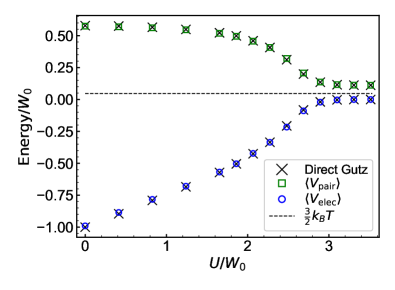
Figure 1: MD averaged electronic free energy $\langle V_{\textrm{elec}}\rangle$ and pair repulsion energy $\langle V_{\textrm{pair}}\rangle$, for varying Hubbard $U$. At every MD time step, forces are produced by an ML model that emulates the Gutzwiller calculation. The crosses represent reference simulations that use direct Gutzwiller calculations rather than ML. The dashed line represents the kinetic energy. The energy scale is $W_{0}=-\langle V_{\textrm{elec}}\rangle|_{U=0}=4.84\,\textrm{eV}$. Tests show that these results with $N=100$ atoms are representative of $N\rightarrow\infty$.

The neural network $\hat{V}_{\textrm{elec},i}$ is composed of multiple real-valued activations $\{z_{m}^{\ell}\}_{m=1\dots M_{\ell}}$ for layer index $\ell=0\dots L$. The input to the neural network is the feature vector, $z_{m}^{\ell=0}=G_{i,m}$. Each neural network layer has the form, $z_{m}^{\ell+1}=f_{\textrm{activ}}(\sum_{n=1}^{M_{\ell}}w_{mn}^{\ell}z_{n}^{\ell}+b_{m}^{\ell})$. The matrix elements $w_{mn}^{\ell}$ and offsets $b_{m}^{\ell}$ are learnable parameters. We select $f_{\textrm{activ}}(x)$ to be the continuously differentiable exponential linear unit (CELU) Barron (2017). A linear combination of the outputs of the final layer yields the local potential, $\hat{V}_{\textrm{elec};i}=\sum_{n=1}^{M_{L}}w_{n}^{L}z_{n}^{L}+b^{L}$. We select $L=3$ and layer sizes $M_{0}=96$, $M_{1}=48$, $M_{2}=32$, and $M_{3}=16$. There are thus approximately $10^{4}$ learnable parameters in this neural network.

Training of the model parameters involves optimizing a loss function $\mathcal{L}$ that quantifies the deviation between the model $\hat{V}_{\textrm{elec}}$ and direct Gutzwiller calculations $V_{\textrm{elec}}$, evaluated on a training dataset. The loss function incorporates errors in the potential, $\hat{V}_{\textrm{elec}}-V_{\textrm{elec}}$ and forces $\nabla_{\mathbf{r}_{i}}(\hat{V}_{\textrm{elec}}-V_{\textrm{elec}})$. We optimize the parameters $w_{mn}^{\ell}$ and $b_{m}^{\ell}$ using the adaptive moment estimation (Adam) variant of stochastic gradient descent Kingma and Ba (2014). To mitigate overfitting, we employ weight decay regularization with $\alpha=10^{-6}$ Loshchilov and Hutter (2017) and early stopping. For a general introduction to this ML methodology, see Ref. Goodfellow et al., 2016.

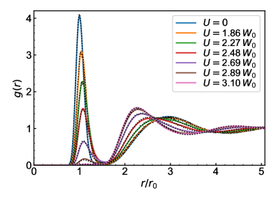
Figure 2: Radial distribution functions $g(r)$ for varying Hubbard $U$, and the same simulation parameters as in Fig. 1. The results using ML (colored lines) are in strong agreement with direct Gutzwiller calculations (black dots). The typical bond length at $U=0$ is $r_{0}=0.83\,\textrm{Å}$.

To produce our training dataset, we ran MD simulations with forces obtained from direct Gutzwiller calculations. We used Verlet integration with a time step of 0.2 fs to evolve the atoms. The simulation box has periodic boundary conditions, and its volume $V_{0}$ is set according to a fixed density $\varrho_{0}=N/V_{0}=0.153\,\textrm{Å}^{-3}$. Just $N=33$ atoms are sufficient to train an extensible ML potential, which remains valid for much larger $N$. To fix the temperature $k_{B}T=0.15\,\textrm{eV}$, we employ a Langevin thermostat with a friction coefficient $\gamma=5\times 10^{-3}\,{\rm amu/fs}$ . We generated independent training data sets for $U$ values ranging from 0 to 17 eV. For each $U$, we collected $3000$ snapshots, one per $200$ MD time steps. Every snapshot contains the electron free energy and associated forces.

We found that an ML model trained on this dataset alone would lead to unstable MD simulations. To improve the robustness of our ML model, we collected additional data that sampled a broader range of the atomic configurations. Specifically, we augmented our training dataset by running additional direct Gutzwiller MD with $k_{B}T=0.075\,\textrm{eV}$ and $k_{B}T=0.3\,\textrm{eV}$ for the Langevin thermostat only, without changing the temperature used in the Gutzwiller equations. Our total training dataset, per $U$ value, thus contains $9,000$ MD snapshots and about $3\times 10^{5}$ atomic forces.

We reduce variance by averaging over an ensemble of eight neural networks, each trained on a subset of the data Smith et al. (2018b).

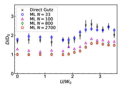
Figure 3: The diffusivity $D$ for varying Hubbard $U$, and the same simulation parameters as in Fig. 1. At $U=0$ with $N=2700$ atoms, we measure $D_{0}=0.0088\,\textrm{Å}^{2}/\textrm{fs}$. Direct Gutzwiller calculations (black crosses) employ five times fewer time steps than used in the ML-based simulations. Approximately $N=800$ atoms are required to reach convergence.

Results. We use our ML models to drive efficient and accurate MD simulations at large scales. Figure 1 shows mean energies for an MD simulation with $N=100$ atoms (keeping $k_{{\rm B}}T=0.15\,\textrm{eV}$) and $3\times 10^{6}$ time steps. The mean electronic energy evaluated at $U=0$ serves as a convenient energy scale, $W_{0}=4.84\,\textrm{eV}$. At large $U$ the electrons become localized, the electronic energy $V_{\textrm{elec}}$ goes to zero, and atoms repel according to $V_{\textrm{pair}}$. At small $U$ the system is metallic and $V_{\textrm{elec}}$ is an attractive interaction that tends to bond atoms into dimer molecules, counterbalanced by $V_{\textrm{pair}}$.

For validation, we also performed reference simulations using forces from direct Gutzwiller calculations at each MD time step, and only $\approx 10^{5}$ time steps. The ML and reference simulations in Fig. 1 are barely distinguishable, which is remarkable given that the training data were generated using only $N=33$ atoms. We also directly compare the ML predictions $\hat{V}_{\textrm{elec}}$ with reference energy calculations $V_{\textrm{elec}}$ for $N=100$ and $N=800$. The mean absolute error (MAE) scales as $0.02\,\sqrt{N}\,W_{0}$. The factor $\sqrt{N}$ appears because the errors in local contributions $\hat{V}_{\textrm{elec};i}$ and $\hat{V}_{\textrm{elec};j}$ are essentially independent for atoms $i\neq j$. The MAE of electronic force $-\nabla\hat{V}_{\textrm{elec}}$ is approximately $0.009\,f_{0}$, where $f_{0}=17.7\,\textrm{eV}/\textrm{Å}$ is the mean force magnitude at $U=0.$ If we were to reduce our training data by a factor of 10, this force MAE would increase by about 10%.

Figure 2 shows the radial distribution functions $g(r)$. At $U=0$, $g(r)$ has a characteristic peak at $r_{0}=0.83\,\mathring{A}$, which reflects the bond length of a dimer molecule. This peak gradually decreases with increasing $U$, and disappears entirely at $U\gtrsim 3.1\,W_{0}$, where $\langle V_{\textrm{elec}}\rangle\approx 0$ according to Fig. 1. The ML-based simulations again appear almost identical to direct-Gutzwiller reference simulations.

Figure 3 shows a dynamic observable, the diffusivity

$$D=\frac{1}{3N}\sum_{i=1}^{N}\int_{0}^{\infty}\langle{\bf v}_{i}(t)\cdot{\bf v}_{i}(0)\rangle\mathrm{d}t.$$ (5)

Replacing $\infty$ with a finite time $\tau$ would yield a naive estimator of $D$. Instead we use an estimator $\hat{D}(\tau)=\frac{1}{2\tau}\frac{1}{3N}\sum_{i}|\int_{0}^{\tau}{\bf v}_{i}(t)dt|^{2}$ with reduced variance. Varying $\tau$, we find that the bias of the estimator $D\approx\langle\hat{D}(\tau_{0})\rangle$ becomes negligible at $\tau_{0}$ corresponding to $10^{5}$ MD time steps. We collected more than ten independent samples of $\hat{D}(\tau_{0})$ from each MD simulation and estimated the error bars using bootstrapping. $D$ converges surprisingly slowly with system size; about $N\approx 800$ atoms seem to be required. Such simulations would have been extremely challenging without ML.

Due to updates in our Gutzwiller solver, the present results deviate significantly from prior work Chern et al. (2017). The mean energies (Fig. 1) and $g(r)$ curves (Fig. 2) now vary smoothly with $U$, indicating a crossover rather than a first-order transition. We also observe in Fig. 3 that $D$ decays smoothly after reaching its peak at the Mott transition, whereas before we had observed a sharp drop. The previous results were dependent on strong hysteresis effects. Here we reinitialize the Gutzwiller parameters at every time step, which eliminates hysteresis and lowers the variational free energy in all instances we checked. We argue that the present approach is more consistent with the assumption (used in the finite-temperature Gutzwiller method) that the electrons are in equilibrium.

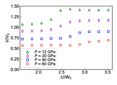
Figure 4: A volume collapse occurs with decreasing $U$. Here we employ an ensemble with constant pressure $P=12,20,40,$ and $80\,\textrm{GPa}$; the pressure of the previous simulations at fixed volume $V_{0}(N)=N/\varrho_{0}$ corresponds to $P=20\,\textrm{GPa}$ when $U\approx 2.4\,W_{0}$. At this temperature, there is a relatively smooth Mott cross-over.

Finally, we investigate the nature of the Mott transition using large-scale MD with $N=2700$ atoms. Here, we switch to an ensemble with constant pressure $P=12,20,40,$ and $80\,\textrm{GPa}$, implemented using the Monte Carlo barostat algorithm Faller and de Pablo (2002). The pressure of our previous (fixed density) simulations matches $P=20\,\textrm{GPa}$ when $U\approx 2.4\,W_{0}$. Figure 4 shows collapse of volume $V$ with decreasing $U$, corresponding to the crossover from the Mott insulating phase to the metallic state.

The ML techniques applied here demonstrate that, with more realistic quantum models, it will be possible to perform large-scale Gutzwiller MD simulations of the structural properties of real f-electron materials, such as Pu, and other correlated electron systems. It is surprising how accurately ML predicts Gutzwiller forces using only the atomic environment within a 2.8 Å radius. The power of ML is that, under the locality assumption, only training data for relatively small system sizes are required. In future work, it should be feasible to generate training data from, e.g., quantum Monte Carlo or DMFT. Once the ML model has been trained, accurate MD simulations of unprecedented scale become practical. For MD boxes with $N=2700$ atoms, our ML model running on a Tesla P100 GPU can evaluate all forces in about 26 ms, which is $\approx 10^{6}$ times faster (extrapolated) than our reference Gutzwiller implementation running on a Intel Xeon CPU E5-2680. We anticipate that a distributed ML/MD implementation could readily enable simulations of $f$-electron materials with millions of atoms.