On the accurate evaluation of unsteady Stokes layer potentials in moving two-dimensional geometries

Abstract

Two fundamental difficulties are encountered in the numerical evaluation of time-dependent layer potentials. One is the quadratic cost of history dependence, which has been successfully addressed by splitting the potentials into two parts - a local part that contains the most recent contributions and a history part that contains the contributions from all earlier times. The history part is smooth, easily discretized using high-order quadratures, and straightforward to compute using a variety of fast algorithms. The local part, however, involves complicated singularities in the underlying Green’s function. Existing methods, based on exchanging the order of integration in space and time, are able to achieve high order accuracy, but are limited to the case of stationary boundaries. Here, we present a new quadrature method that leaves the order of integration unchanged, making use of a change of variables that converts the singular integrals with respect to time into smooth ones. We have also derived asymptotic formulas for the local part that lead to fast and accurate hybrid schemes, extending earlier work for scalar heat potentials and applicable to moving boundaries. The performance of the overall scheme is demonstrated via numerical examples.

Keywords: Unsteady Stokes flow, linearized Navier-Stokes equations, boundary integral equations, asymptotic expansion, layer potentials, moving geometries.

1 Introduction

In this paper, we consider an integral equation approach to the linearized, incompressible Navier-Stokes equations (also called unsteady Stokes flow) in a nonstationary domain $D_{T}=\prod_{\tau=0}^{T}D(\tau)$ with smooth boundary $\Gamma_{T}=\prod_{\tau=0}^{T}\Gamma(\tau)$:

(1.1) $$\frac{\partial{\bf u}}{\partial t} =\Delta{\bf u}-\nabla p+{\bf g},\qquad(\mathbf{x},t)\in D_{T},$$

(1.2) $$\nabla\cdot{\bf u} =0,\qquad(\mathbf{x},t)\in D_{T},$$

(1.3) $${\bf u}(\mathbf{x},0) ={\bf u}_{0}(\mathbf{x}),\qquad\mathbf{x}\in D(0),$$

subject to either Dirichlet (“velocity”) boundary conditions

(1.4) $${\bf u}(\mathbf{x},t)={\bf f}(\mathbf{x},t),\qquad(\mathbf{x},t)\in\Gamma_{T}$$

or Neumann (“traction”) boundary conditions

(1.5) $$\left(\frac{\partial\mathbf{u}_{i}(\mathbf{x},t)}{\partial\mathbf{x}_{k}}+\frac{\partial\mathbf{u}_{k}(\mathbf{x},t)}{\partial\mathbf{x}_{i}}-p(\mathbf{x},t)\delta_{ik}\right)\mathbf{n}_{k}(\mathbf{x})=\mathbf{f}(\mathbf{x},t),\qquad(\mathbf{x},t)\in\Gamma_{T}.$$

While unsteady Stokes flow is of interest in its own right in modeling slow viscous flow, with applications in microfluidics [16, 17], it also arises in solving the fully nonlinear incompressible Navier-Stokes equations, where ${\bf g}=-{\bf u}\cdot\nabla{\bf u}$. In fact, most widely used marching schemes for the nonlinear problem treat the advective term explicitly so that ${\bf g}(\mathbf{x},t)$ can be considered a known function when marching in time [2, 4, 5, 14, 22, 26].

We are interested here in methods for the unsteady Stokes equations that enforce the divergence-free condition exactly, without the need for a projection step. Recently, we described a “mixed potential” method that accomplishes this task through a Helmholtz decomposition of the forcing term ${\bf g}$ [8]. In the present paper, we continue our investigation, begun in [15], of integral equation methods that rely on the Green’s function for the unsteady Stokes equations - the so-called unsteady Stokeslet. We will discuss the relative merits of the mixed potential approach and the unsteady Stokeslet-based approach in the concluding section. For the moment, we simply note that initial, volume, and layer potentials based on the unsteady Stokeslet involve nothing more than convolution with the Green’s function without any Helmholtz decomposition. Moreover, standard velocity or traction boundary conditions can be imposed using the double layer or single layer potential, respectively. These lead to well-conditioned integral equations of Volterra type.

For stationary boundaries, high-order accurate quadrature schemes have also developed [15], following the approach developed for layer heat potentials in [9, 20, 21]. That is, the layer potentials are split into two parts - a local part and a history part, where the local part contains the temporal integration on the interval $[t-\delta,t]$ and the history part contains the temporal integration on $[0,t-\delta]$. The local part involves essential singularities in time, treated by exchanging the order of integration in space and time, and carrying out product integration in time analytically. The history part requires fast algorithms, but is more or less straightforward to discretize since the integrals encountered are smooth in time.

When the boundary is nonstationary, the aforementioned scheme can still be used to evaluate heat layer potentials accurately. As observed in [20], the heat kernel admits the following factorization:

(1.6) $$G_{H}(\mathbf{x},t;\mathbf{y}(\tau),\tau) =\frac{1}{4\pi(t-\tau)}e^{-\frac{\|\mathbf{x}-\mathbf{y}(\tau)\|^{2}}{4(t-\tau)}}$$

$$=\frac{1}{4\pi(t-\tau)}e^{-\frac{\|\mathbf{x}(t)-\mathbf{y}(t)\|^{2}}{4(t-\tau)}}\cdot e^{-\frac{\|\mathbf{y}(t)-\mathbf{y}(\tau)\|^{2}}{4(t-\tau)}}\cdot e^{-\frac{(\mathbf{x}(t)-\mathbf{y}(t))\cdot(\mathbf{y}(t)-\mathbf{y}(\tau))}{2(t-\tau)}}.$$

Note that the first term on the right side of Eq. 1.6 can be dealt with via product integration, as in the stationary case, while the second and third terms are both smooth so long as the boundary motion is smooth, since the factor $\frac{\mathbf{y}(t)-\mathbf{y}(\tau)}{(t-\tau)}$ is then well behaved as a function of $\tau$. Unfortunately, this simple modification fails for unsteady Stokes layer potentials. The unsteady Stokeslet $\mathbf{G}(\mathbf{x},t;\mathbf{y},\tau)$ [11, 15] is given by the formula

(1.7) $$\mathbf{G}(\mathbf{x},t;\mathbf{y},\tau) =\frac{e^{-\|\mathbf{r}\|^{2}/4(t-\tau)}}{4\pi(t-\tau)}\left(\mathbf{I}-\frac{\mathbf{r}\otimes\mathbf{r}}{\|\mathbf{r}\|^{2}}\right)-\frac{1-e^{-\|\mathbf{r}\|^{2}/4(t-\tau)}}{2\pi\|\mathbf{r}\|^{2}}\left(\mathbf{I}-2\frac{\mathbf{r}\otimes\mathbf{r}}{\|\mathbf{r}\|^{2}}\right),$$

where $\mathbf{r}=\mathbf{x}-\mathbf{y}$. As a result, when the boundary is moving, $\mathbf{r}=\mathbf{x}-\mathbf{y}(\tau)$ and the first term can be handled as above but the second term on the right-hand side of Eq. 1.7 cannot be factorized as a Stokeslet on a fixed domain modulated by a smooth function, due to the presence of the factor $\|\mathbf{r}\|^{2}$ in the denominator.

Here, we present an accurate numerical scheme for the evaluation of the local part of the unsteady Stokes layer potentials for both static and moving geometries. For this, we split the local part further into two parts: $[t-\delta,t]=[t-\delta,t-\epsilon]\cup[t-\epsilon,t]$ - the second part is treated asymptotically and the interval $[{t-\delta},{t-\epsilon}]$ is treated by a change of variables in the nearly singular integrals, as in [28]. We carry out the asymptotic analysis only to lowest order for both the single and double layer potentials. The double layer derivation is somewhat technical as compared with the double layer heat potential [10, 28] because the kernel is not Riemann-integrable and defined only in the principal value sense. Furthermore, although the first asymptotic term, of the order $\sqrt{\epsilon}$, is local in space-time, the next term of order $O(\epsilon)$ involves an integral on the entire spatial boundary. By contrast, asymptotic expansions for heat layer potentials involves terms which remain local (although they involve higher and higher order spatial derivatives for higher and higher powers of $\epsilon$.)

An important difference between the current approach and the earlier method of [15] is that the spatial integrals are now singular rather than weakly singular and have to be interpreted in the principal value sense. Fortunately, there are many high-order rules available, such as the Gauss-trapezoidal rule of [1]. After combining all these tools, the overall scheme is high-order accurate even for nonstationary boundaries and the linear systems which arise from implicit time-marching schemes are well-conditioned and amenable to solution using iterative schemes such as GMRES [24].

The paper is organized as follows. In section 2, we state some needed integral identities and summarize the relevant properties of single and double layer potentials for unsteady Stokes flow. In section 3, we derive the leading order asymptotic expansions for layer potentials and in section 4, we discuss the numerical treatment of the nearly-singular parts. In section 5, a fully discrete numerical scheme is described for the Dirichlet problem. Numerical examples are presented in section 6 with some concluding remarks in section 7.

2 Mathematical preliminaries

We turn now to a brief summary of potential theory for unsteady Stokes flow. We refer the reader to [6, 7, 25] for a detailed analysis of the properties of these parabolically singular layer potentials.

Definition 1.

Let $\boldsymbol{\phi}$ be a vector-valued function defined on $\Gamma_{T}$. Then the single layer potential operator $\mathcal{S}$ is defined by the formula

(2.1) $$\mathcal{S}[\boldsymbol{\phi}](\mathbf{x},t)=\int_{0}^{t}\int_{\Gamma(\tau)}\mathbf{G}(\mathbf{x},t;\mathbf{y},\tau)\mathbf{\boldsymbol{\phi}}(\mathbf{y},\tau)ds(\mathbf{y})d\tau,$$

where $\mathbf{G}(\mathbf{x},t;\mathbf{y},\tau)$ is defined in Eq. 1.7. The double layer potential operator $\mathcal{D}$ is defined by the formula

(2.2) $$\mathcal{D}[\boldsymbol{\phi}](\mathbf{x},t)=\int_{0}^{t}\int_{\Gamma(\tau)}\mathbf{D}(\mathbf{x},t;\mathbf{y},\tau)\mathbf{\boldsymbol{\phi}}(\mathbf{y},\tau)ds(\mathbf{y})d\tau+\int_{\Gamma(t)}\frac{\mathbf{r}\otimes\mathbf{n}(\mathbf{y})}{2\pi\|\mathbf{r}\|^{2}}\mathbf{\boldsymbol{\phi}}(\mathbf{y},t)ds(\mathbf{y}),$$

where

(2.3) $$\mathbf{D}(\mathbf{x},t;\mathbf{y},\tau) =\frac{\mathbf{n}(\mathbf{y})\otimes\mathbf{r}+(\mathbf{n}(\mathbf{y})\cdot\mathbf{r})(\mathbf{I}-2\frac{\mathbf{r}\otimes\mathbf{r}}{\|\mathbf{r}\|^{2}})}{8\pi}\frac{e^{-\lambda}}{(t-\tau)^{2}}$$

$$-\frac{\mathbf{n}(\mathbf{y})\otimes\mathbf{r}+\mathbf{r}\otimes\mathbf{n}(\mathbf{y})+(\mathbf{n}(\mathbf{y})\cdot\mathbf{r})(\mathbf{I}-4\frac{\mathbf{r}\otimes\mathbf{r}}{\|\mathbf{r}\|^{2}})}{8\pi}\frac{1-e^{-\lambda}-\lambda e^{-\lambda}}{\lambda^{2}(t-\tau)^{2}},$$

with $\lambda=\frac{\|\mathbf{r}\|^{2}}{4(t-\tau)}$. The kernel in the second term of Eq. 2.2 is the contribution of the instantaneous pressurelet $\mathbf{p}(\mathbf{x},t;\mathbf{y},\tau)$, denoted by

(2.4) $$\mathbf{p}(\mathbf{x},t;\mathbf{y},\tau)=\frac{\mathbf{r}}{2\pi\|\mathbf{r}\|^{2}}\delta(t-\tau),$$

where the Dirac $\delta$ function is understood to satisfy the condition $\int_{0}^{t}\delta(t-\tau)d\tau=1$.

We decompose the single layer potential $\mathcal{S}[\boldsymbol{\phi}]$ defined in Eq. 2.1 into two parts - a local part and a history part:

(2.5) $$\mathcal{S}[\boldsymbol{\phi}]=\mathcal{S}_{L}[\boldsymbol{\phi}]+\mathcal{S}_{H}[\boldsymbol{\phi}],$$

where the local part is

(2.6) $$\mathcal{S}_{L}[\boldsymbol{\phi}](\mathbf{x},t)=\int_{t-\delta}^{t}\int_{\Gamma(\tau)}\mathbf{G}(\mathbf{x},t;\mathbf{y},\tau)\boldsymbol{\phi}(\mathbf{y},\tau)ds(\mathbf{y})d\tau,$$

and the history part is

(2.7) $$S_{H}[\boldsymbol{\phi}](\mathbf{x},t)=\int_{0}^{t-\delta}\int_{\Gamma(\tau)}\mathbf{G}(\mathbf{x},t;\mathbf{y},\tau)\boldsymbol{\phi}(\mathbf{y},\tau)ds(\mathbf{y})d\tau.$$

It is convenient to split the double layer potential $\mathcal{D}[\boldsymbol{\phi}]$ into three parts: a local part $\mathcal{D}_{L}[\boldsymbol{\phi}]$, a history part $\mathcal{D}_{H}[\boldsymbol{\phi}]$, and a pressure part $\mathcal{D}_{P}[\boldsymbol{\phi}]$:

(2.8) $$\mathcal{D}[\boldsymbol{\phi}]=\mathcal{D}_{L}[\boldsymbol{\phi}]+\mathcal{D}_{H}[\boldsymbol{\phi}]+\mathcal{D}_{P}[\boldsymbol{\phi}]$$

with

$$\mathcal{D}_{L}[\boldsymbol{\phi}] :=\int_{t-\delta}^{t}\int_{\Gamma(\tau)}\mathbf{D}(\mathbf{x},t;\mathbf{y},\tau)\boldsymbol{\phi}(\mathbf{y},\tau)ds(\mathbf{y})d\tau,$$

$$\mathcal{D}_{H}[\boldsymbol{\phi}] :=\int_{0}^{t-\delta}\int_{\Gamma(\tau)}\mathbf{D}(\mathbf{x},t;\mathbf{y},\tau)\boldsymbol{\phi}(\mathbf{y},\tau)ds(\mathbf{y})d\tau,$$

$$\mathcal{D}_{P}[\boldsymbol{\phi}] :=\int_{\Gamma(t)}\frac{\mathbf{r}\otimes\mathbf{n}(\mathbf{y})}{2\pi\|\mathbf{r}\|^{2}}\mathbf{\boldsymbol{\phi}}(\mathbf{y},t)ds(\mathbf{y}),$$

where the first and third terms on the right side of Eq. 2.8 are understood in the principal value sense. For both layer potentials, the parameter $\delta$ will be chosen to be a constant multiple of whatever time step $\Delta t$ is being used in a time-marching scheme. The density $\boldsymbol{\phi}$, will be represented by a piecewise polynomial approximation with respect to the time variable. The degree of that approximation determines the time order of accuracy of the numerical scheme [15].

We will make use of the following integral identities:

(2.9) $$\int_{-\infty}^{\infty}e^{-z^{2}}dz=\sqrt{\pi},\quad\int_{-\infty}^{\infty}z^{2}e^{-z^{2}}dz =\frac{\sqrt{\pi}}{2},$$

(2.10) $$\int_{-\infty}^{\infty}\frac{1-e^{-z^{2}}}{z^{2}}dz =2\sqrt{\pi},$$

(2.11) $$\int_{-\infty}^{\infty}\frac{1-e^{-z^{2}}-z^{2}e^{-z^{2}}}{z^{4}}dz =\frac{2\sqrt{\pi}}{3}.$$

The formulas Eq. 2.9 are well-known. To prove Eq. 2.10, let $f(x)$ be defined by the formula

(2.12) $$f(x)=\int_{-\infty}^{\infty}\frac{1-e^{-xz^{2}}}{z^{2}}dz.$$

It is easy to show that $f(x)$ is well defined for $x\in(0,+\infty)$ since the integrand is bounded as $z\rightarrow 0$ and integrable as $z\rightarrow\pm\infty$. Moreover, calculation shows that $\lim_{x\rightarrow 0^{+}}f(x)=0$ and $f^{\prime}(x)=\int_{-\infty}^{\infty}e^{-xz^{2}}dz=\frac{\sqrt{\pi}}{\sqrt{x}}$ for $x>0$. Integrating $f^{\prime}(x)$ from $0$ to $1$, we obtain Eq. 2.10. Similarly, let $g(x)$ be defined by

(2.13) $$g(x)=\int_{-\infty}^{\infty}\frac{1-e^{-xz^{2}}-xz^{2}e^{-xz^{2}}}{z^{4}}dz.$$

Then $\lim_{x\rightarrow 0^{+}}g(x)=0$ and $g^{\prime}(x)=\int_{-\infty}^{\infty}xe^{-xz^{2}}dz=\sqrt{\pi x}$ for $x>0$. Integrating $g^{\prime}(x)$ from $0$ to $1$, we obtain Eq. 2.11.

Remark 1.

To solve the equations Eq. 1.1 with velocity boundary conditions, we seek a representation of the solution of the form

$${\bf u}(\mathbf{x},t)=\mathcal{D}[\boldsymbol{\phi}](\mathbf{x},t)+{\cal V}[{\bf g}](\mathbf{x},t),$$

where

$${\cal V}[{\bf g}](\mathbf{x},t)=\int_{0}^{t}\int_{\Omega(\tau)}\mathbf{G}(\mathbf{x},t;\mathbf{y},\tau)\bf{g}(\mathbf{y},\tau)\,d\mathbf{y}\,d\tau.$$

This satisfies the partial differential equation and divergence condition bu construction [15]. Imposition of the boundary condition Eq. 1.4 leads to the boundary integral equation

(2.14) $$-\frac{1}{2}\boldsymbol{\phi}(\mathbf{x},t)+\mathcal{D}^{\ast}[\boldsymbol{\phi}](\mathbf{x},t)={\bf f}(\mathbf{x},t)-{\cal V}[{\bf g}](\mathbf{x},t)$$

where $\mathcal{D}^{\ast}[\boldsymbol{\phi}](\mathbf{x},t)$ denotes the double layer potential defined in the principal value sense. We are primarily interested here in the solution of this equation and the design of suitable quadrature methods and will assume that the the volume source term and corresponding potential ${\cal V}[{\bf g}](\mathbf{x},t)$ are absent for the sake of simplicity.

3 Asymptotic analysis of the local layer potentials

While it is possible to treat the local parts of the single and double layer potentials by quadrature techniques alone, it will turn out to be more efficient to split them further in the form:

(3.1) $$\mathcal{S}_{L}[\boldsymbol{\phi}]=\mathcal{S}_{\epsilon}[\boldsymbol{\phi}]+\mathcal{S}_{N}[\boldsymbol{\phi}]$$

and

(3.2) $$\mathcal{D}_{L}[\boldsymbol{\phi}]=\mathcal{D}_{\epsilon}[\boldsymbol{\phi}]+\mathcal{D}_{N}[\boldsymbol{\phi}]$$

where

$$\mathcal{S}_{\epsilon}[\boldsymbol{\phi}] :=\int_{t-\epsilon}^{t}\int_{\Gamma(\tau)}\mathbf{G}(\mathbf{x},t;\mathbf{y},\tau)\boldsymbol{\phi}(\mathbf{y},\tau)ds(\mathbf{y})d\tau,$$

$$\mathcal{S}_{N}[\boldsymbol{\phi}] :=\int_{t-\delta}^{t-\epsilon}\int_{\Gamma(\tau)}\mathbf{G}(\mathbf{x},t;\mathbf{y},\tau)\boldsymbol{\phi}(\mathbf{y},\tau)ds(\mathbf{y})d\tau,$$

$$\mathcal{D}_{\epsilon}[\boldsymbol{\phi}] :=\int_{t-\epsilon}^{t}\int_{\Gamma(\tau)}\mathbf{D}(\mathbf{x},t;\mathbf{y},\tau)\boldsymbol{\phi}(\mathbf{y},\tau)ds(\mathbf{y})d\tau$$

$$\mathcal{D}_{N}[\boldsymbol{\phi}] :=\int_{t-\delta}^{t-\epsilon}\int_{\Gamma(\tau)}\mathbf{D}(\mathbf{x},t;\mathbf{y},\tau)\boldsymbol{\phi}(\mathbf{y},\tau)ds(\mathbf{y})d\tau.$$

The terms $\mathcal{S}_{\epsilon}[\boldsymbol{\phi}]$ and $\mathcal{D}_{\epsilon}[\boldsymbol{\phi}]$ will be treated by asymptotic methods, with $\epsilon$ chosen to be sufficiently small to satisfy a given error tolerance.

To carry out the analysis, let the reference “target” point be denoted by $\mathbf{x}\in\Gamma(t)$. The unit tangent vector, unit normal vector and signed curvature at $\mathbf{x}$ are denoted by $\mathbf{T}$, $\mathbf{n}$, and $\kappa$, respectively. The velocity at $(\mathbf{x},t)$ is denoted by $\mathbf{v}$. Assuming the curve is parametrized in arclength $s$, starting from $\mathbf{x}$, the “source” point $\mathbf{y}(s,\tau)\in\Gamma(\tau)$ has the following Taylor expansion in $s$ and $t-\tau$:

(3.3) $$\mathbf{y}(s,\tau)=\mathbf{x}+\mathbf{T}s-\frac{1}{2}\mathbf{n}\,\kappa s^{2}-(\mathbf{v}\cdot\mathbf{n})\mathbf{n}(t-\tau)+\cdots.$$

Lemma 1.

The leading order asymptotic expansion of the single layer potential is given by

(3.4) $$\mathcal{S}_{\epsilon}[\boldsymbol{\phi}](\mathbf{x},t)=\sqrt{\frac{\epsilon}{\pi}}\mathbf{T}\otimes\mathbf{T}\boldsymbol{\phi}(\mathbf{x},t)+O(\epsilon).$$

Proof.

We first split the spatial integral in $\mathcal{S}_{\epsilon}[\boldsymbol{\phi}]$ into two parts:

(3.5) $$\int_{\Gamma(\tau)}=\int_{\Gamma(\tau)\cap B_{a}^{c}(\mathbf{x})}+\int_{\Gamma(\tau)\cap B_{a}(\mathbf{x})},$$

where $B_{a}(\mathbf{x})$ is a ball of radius $a$ centered at $\mathbf{x}$ and $B_{a}^{c}(\mathbf{x})$ is its complement in $\mathbb{R}^{2}$. Here, $a$ is a fixed small positive number. Clearly, $\|\mathbf{r}\|$ is bounded away from zero on $\Gamma(\tau)\cap B_{a}^{c}(\mathbf{x})$. Thus, the term $\frac{e^{-\|\mathbf{r}\|^{2}/4(t-\tau)}}{4\pi(t-\tau)}\rightarrow 0$ exponentially fast as $\epsilon\rightarrow 0$ for $\tau\in(t-\epsilon,t)$, and the term $\frac{1-e^{-\|\mathbf{r}\|^{2}/4(t-\tau)}}{2\pi\|\mathbf{r}\|^{2}}$ approaches $\frac{1}{2\pi\|\mathbf{r}\|^{2}}$. Combining these two facts, we conclude that

(3.6) $$\int_{t-\epsilon}^{t}\int_{\Gamma(\tau)\cap B_{a}^{c}(\mathbf{x})}\sim O(\epsilon),$$

and hence,

(3.7) $$\mathcal{S}_{\epsilon}[\boldsymbol{\phi}](\mathbf{x},t)=\int_{t-\epsilon}^{t}\int_{\Gamma(\tau)\cap B_{a}(\mathbf{x})}\mathbf{G}(\mathbf{x},t;\mathbf{y},\tau)\boldsymbol{\phi}(\mathbf{y},\tau)ds(\mathbf{y})d\tau+O(\epsilon).$$

In the following asymptotic estimates, we assume $s^{2}=O(t-\tau)$.

(3.8) $$\mathbf{r} =\mathbf{x}-\mathbf{y}=-\mathbf{T}s+\frac{1}{2}\mathbf{n}\kappa s^{2}+(\mathbf{v}\cdot\mathbf{n})\mathbf{n}(t-\tau)+\cdots,$$

$$\|\mathbf{r}\|^{2} =s^{2}+O(s^{3}),\qquad\frac{\mathbf{r}\otimes\mathbf{r}}{\|\mathbf{r}\|^{2}}=\mathbf{T}\otimes\mathbf{T}+O(s),\qquad ds(\mathbf{y})=(1+O(s^{2}))ds.$$

Substituting Eq. 3.8 into Eq. 3.7, we obtain

(3.9) $$\mathcal{S}_{\epsilon}[\boldsymbol{\phi}](\mathbf{x},t)=\int_{t-\epsilon}^{t}\int_{-a}^{a}\left(\frac{e^{-s^{2}/4(t-\tau)+O(s)}}{4\pi(t-\tau)}\left(\mathbf{I}-\mathbf{T}\otimes\mathbf{T}+O(s)\right)\right.$$

$$\left.-\frac{1-e^{-s^{2}/4(t-\tau)+O(s)}}{2\pi s^{2}}\left(\mathbf{I}-2\mathbf{T}\otimes\mathbf{T}+O(s)\right)\right)\boldsymbol{\phi}(\mathbf{y},\tau)(1+O(s^{2}))dsd\tau+O(\epsilon).$$

The change of variables $z=\frac{s}{\sqrt{4(t-\tau)}}$ and $u=\sqrt{4(t-\tau)}$ gives $s=zu$, $\tau=t-u^{2}/4$, $dsd\tau=-2(t-\tau)dzdu$. Thus,

(3.10) $$\mathcal{S}_{\epsilon}[\boldsymbol{\phi}](\mathbf{x},t)=2\int_{0}^{2\sqrt{\epsilon}}\int_{-\infty}^{\infty}\left(\frac{e^{-z^{2}}}{4\pi}\left(\mathbf{I}-\mathbf{T}\otimes\mathbf{T}\right)\right.$$

$$\left.-\frac{1-e^{-z^{2}}}{8\pi z^{2}}\left(\mathbf{I}-2\mathbf{T}\otimes\mathbf{T}\right)\right)\boldsymbol{\phi}(\mathbf{y}(zu,t-u^{2}/4),t-u^{2}/4)dzdu+O(\epsilon).$$

Note that $\mathbf{x}=\mathbf{y}(0,t)$. Substituting Eqs. 2.9 and 2.10 into the above expression, we obtain

(3.11) $$\mathcal{S}_{\epsilon}[\boldsymbol{\phi}](\mathbf{x},t)=4\sqrt{\epsilon}\left(\frac{\sqrt{\pi}}{4\pi}\left(\mathbf{I}-\mathbf{T}\otimes\mathbf{T}\right)-\frac{\sqrt{\pi}}{4\pi}\left(\mathbf{I}-2\mathbf{T}\otimes\mathbf{T}\right)\right)\boldsymbol{\phi}(\mathbf{x},t)+O(\epsilon),$$

from which the result follows. ∎

Lemma 2.

The leading order asymptotic expansion of the double layer potential is given by

(3.12) $$\mathcal{D}_{\epsilon}[\boldsymbol{\phi}](\mathbf{x},t) =\int_{t-\epsilon}^{t}\int_{\Gamma(\tau)}\mathbf{D}(\mathbf{x},t;\mathbf{y},\tau)\boldsymbol{\phi}(\mathbf{y},\tau)ds(\mathbf{y})d\tau$$

$$=\sqrt{\frac{\epsilon}{\pi}}\left\{\left(\frac{1}{6}\mathbf{v}\cdot\mathbf{n}+\frac{1}{2}\kappa\right)\mathbf{I}+\frac{1}{3}(\mathbf{v}\cdot\mathbf{n})\mathbf{T}\otimes\mathbf{T}\right.$$

$$\left.-\left(\frac{\mathbf{v}\cdot\mathbf{n}}{6}+\frac{3\kappa}{2}\right)\mathbf{n}\otimes\mathbf{n}\right\}\boldsymbol{\phi}(\mathbf{x},t)$$

$$+\sqrt{\frac{\epsilon}{\pi}}\left\{\mathbf{n}\otimes\mathbf{T}+2\mathbf{T}\otimes\mathbf{n}\right\}\boldsymbol{\phi}_{s}(\mathbf{x},t)+O(\epsilon).$$

Proof.

Analysis of the double layer is more involved because of the fact that it is defined only in the principal value sense. We proceed by first expanding various needed quantities in terms of the arclength parameter $s$:

$$\mathbf{r}=\mathbf{x}-\mathbf{y}=-\mathbf{T}s+\frac{1}{2}\mathbf{n}\kappa s^{2}+(\mathbf{v}\cdot\mathbf{n})\mathbf{n}(t-\tau)+O(s^{3}),$$

$$\mathbf{n}(\mathbf{y})=\mathbf{n}+\mathbf{T}\kappa s+O(s^{2}),$$

(3.13) $$\mathbf{n}(\mathbf{y})\cdot\mathbf{r}=-\frac{1}{2}\kappa s^{2}+(\mathbf{v}\cdot\mathbf{n})(t-\tau)+O(s^{3}),$$

$$\mathbf{n}(\mathbf{y})\otimes\mathbf{r}=-\mathbf{n}\otimes\mathbf{T}s+\left(\frac{1}{2}\mathbf{n}\otimes\mathbf{n}-\mathbf{T}\otimes\mathbf{T}\right)\kappa s^{2}+(\mathbf{v}\cdot\mathbf{n})\mathbf{n}\otimes\mathbf{n}(t-\tau)+O(s^{3}),$$

$$\mathbf{r}\otimes\mathbf{n}(\mathbf{y})=-\mathbf{T}\otimes\mathbf{n}s+\left(\frac{1}{2}\mathbf{n}\otimes\mathbf{n}-\mathbf{T}\otimes\mathbf{T}\right)\kappa s^{2}+(\mathbf{v}\cdot\mathbf{n})\mathbf{n}\otimes\mathbf{n}(t-\tau)+O(s^{3}),$$

$$\boldsymbol{\phi}(\mathbf{y},\tau)=\boldsymbol{\phi}(\mathbf{x},t)+\boldsymbol{\phi}_{s}(\mathbf{x},t)s+O(s^{2}).$$

In the last expression, $\boldsymbol{\phi}_{s}$ is the derivative of $\boldsymbol{\phi}$ with respect to arclength. Using the same change of variables as for the single layer, namely $z=\frac{s}{\sqrt{4(t-\tau)}}$ and $u=\sqrt{4(t-\tau)}$, we have

(3.14) $$\int_{t-\epsilon}^{t}\int_{-\infty}^{\infty}s^{2}\frac{e^{-s^{2}/4(t-\tau)}}{(t-\tau)^{2}}dsd\tau=8\int_{0}^{2\sqrt{\epsilon}}\int_{-\infty}^{\infty}z^{2}e^{-z^{2}}dzdu=8\sqrt{\pi\epsilon},$$

(3.15) $$\int_{t-\epsilon}^{t}\int_{-\infty}^{\infty}(t-\tau)\frac{e^{-s^{2}/4(t-\tau)}}{(t-\tau)^{2}}dsd\tau=2\int_{0}^{2\sqrt{\epsilon}}\int_{-\infty}^{\infty}e^{-z^{2}}dzdu=4\sqrt{\pi\epsilon},$$

(3.16) $$\int_{t-\epsilon}^{t}\int_{-\infty}^{\infty}s^{2}\frac{1-e^{-s^{2}/4(t-\tau)}-s^{2}/(4(t-\tau))e^{-s^{2}/4(t-\tau)}}{(s^{2}/(4(t-\tau)))^{2}(t-\tau)^{2}}dsd\tau=16\sqrt{\pi\epsilon},$$

(3.17) $$\int_{t-\epsilon}^{t}\int_{-\infty}^{\infty}(t-\tau)\frac{1-e^{-s^{2}/4(t-\tau)}-s^{2}/(4(t-\tau))e^{-s^{2}/4(t-\tau)}}{(s^{2}/(4(t-\tau)))^{2}(t-\tau)^{2}}dsd\tau=\frac{8}{3}\sqrt{\pi\epsilon}.$$

The desired result follows from combining Eqs. 2.3, 3.2, 3.8, 3.13, 3.14, 3.15, 3.16 and 3.17 after simplifying the resulting expression. ∎

4 Quadrature methods for the nearly singular parts

We now consider the evaluation of the nearly singular contributions to the single and double layer potentials, $\mathcal{S}_{N}[\boldsymbol{\phi}]$ and $\mathcal{D}_{N}[\boldsymbol{\phi}]$. Inspection of the kernels shows that we need to consider the following terms which involve singularities in either space or time:

(4.1) $$\frac{\mathbf{r}\otimes\mathbf{r}}{\|\mathbf{r}\|^{2}},\qquad\frac{e^{-\lambda}}{t-\tau},\qquad\frac{e^{-\lambda}}{(t-\tau)^{2}},\qquad\frac{1-e^{-\lambda}}{\lambda(t-\tau)},\qquad\frac{1-e^{-\lambda}-\lambda e^{-\lambda}}{\lambda^{2}(t-\tau)^{2}},$$

where $\lambda=\frac{\|\mathbf{r}\|^{2}}{4(t-\tau)}$.

Each entry in the tensor product $\frac{\mathbf{r}\otimes\mathbf{r}}{\|\mathbf{r}\|^{2}}$ is bounded by $1$ but does not have a definite limiting value as $\|\mathbf{r}\|\rightarrow 0$. In [15], it was shown that by carrying out product integration in time first, the resulting spatial convolution kernels have logarithmic singularities for which there are effective quadrature rules. The full double layer kernel (including the pressurelet) involves non-integrable singularities, so it is critical to use quadrature rules that integrate functions in the principal value sense as well. Alpert’s Gauss-trapezoidal rule for logarithmic singularities [1] accomplishes both tasks with very high order accuracy for discretizations based on equispaced points with respect to an underlying parametrization of the curve $\Gamma(t)$. For adaptive methods, based on representing the boundary as the concatenation of boundary segments, a variety of other high-order rules are available [3, 18, 23, 29, 12, 13, 19]. In all cases, the spatial quadrature rules avoid kernel evaluation at the singular point $\mathbf{r}={\bf 0}$ itself. Thus, we will assume that $\mathbf{r}\neq{\bf 0}$ in the subsequent discussion.

The remaining four terms in Eq. 4.1 involve singularities in time. We need to integrate these terms when multiplied by a smooth function of $\tau$ on the interval $[t-\delta,t-\epsilon]$. Assuming for simplicity that the smooth function is constant, we follow the approach introduced for heat potentials in [28] and apply the change of variables $t-\tau=e^{z}$. Assuming the smooth function is constant as a function of $\tau$, we have

(4.2) $$\int_{t-\delta}^{t-\epsilon}\frac{e^{-\lambda}}{t-\tau}d\tau =\int_{\ln\epsilon}^{\ln\delta}e^{-\frac{\|\mathbf{r}\|^{2}}{4}e^{-z}}dz,$$

$$\int_{t-\delta}^{t-\epsilon}\frac{e^{-\lambda}}{(t-\tau)^{2}}d\tau =\int_{\ln\epsilon}^{\ln\delta}e^{-\frac{\|\mathbf{r}\|^{2}}{4}e^{-z}}e^{-z}dz,$$

$$\int_{t-\delta}^{t-\epsilon}\frac{1-e^{-\lambda}}{\lambda(t-\tau)}d\tau =\int_{\ln\epsilon}^{\ln\delta}\frac{4}{\|\mathbf{r}\|^{2}}\left(1-e^{-\frac{\|\mathbf{r}\|^{2}}{4}e^{-z}}\right)e^{z}dz,$$

$$\int_{t-\delta}^{t-\epsilon}\frac{1-e^{-\lambda}-\lambda e^{-\lambda}}{\lambda^{2}(t-\tau)^{2}}d\tau =\int_{\ln\epsilon}^{\ln\delta}\frac{16}{\|\mathbf{r}\|^{4}}\left(1-e^{-\frac{\|\mathbf{r}\|^{2}}{4}e^{-z}}-\frac{\|\mathbf{r}\|^{2}}{4}e^{-z}e^{-\frac{\|\mathbf{r}\|^{2}}{4}e^{-z}}\right)e^{z}dz.$$

Note that all of the integrals in Eq. 4.2 are smooth in the new variable $z$ (even for $\mathbf{r}={\bf 0}$). Following [28], in which only the first two integrals above arise, we use Gauss-Legendre quadrature on the interval $[\ln\epsilon,\ln\delta]$ to compute these integrals and the corresponding temporal integration in both $\mathcal{S}_{N}[\boldsymbol{\phi}]$ and $\mathcal{D}_{N}[\boldsymbol{\phi}]$. A detailed analysis of the discretization error is nontrivial even for the case of the scalar heat kernel. It is shown in [28], however, that the error in $n$-point Gauss-Legendre quadrature for the single layer potential is of the order $O(\Delta t^{k})+O\left(\log\left(\frac{\Delta t}{\epsilon}\right)\,f(n)\right)$, where $f(n)$ is an exponentially decreasing function of $n$. The first term accounts for the use of a k$th$ order accurate approximation of the density in time. The second term is more subtle. The order of accuracy is low with respect to the time step but compensated for by permitting controllable precision by increasing $n$. Our numerical experiments are consistent with the estimate above, but in practice, local error estimation based on the desired precision will more efficiently determine the number of nodes required than a priori analysis. Numerical experiments show that the number of quadrature points needed is about $10\log_{10}(1/\epsilon)$ to achieve a precision of $\epsilon$ for $\|\mathbf{r}\|\in[0,1]$, assuming that $\|\mathbf{r}\|$ is a smoothly varying function of $\tau$. It is likely that we could reduce the number of nodes needed by a more specialized generalized Gaussian rule [3, 23, 29].

5 Numerical Implementation

We illustrate the use of our hybrid scheme in solving the problem of unsteady Stokes flow with velocity boundary conditions. The procedure follows that in [15], and we refer the reader to that paper for a detailed discussion. In short, for the history part $\mathcal{D}_{H}[\boldsymbol{\phi}]$, we make use of a Fourier spectral approximation of the unsteady Stokeslet. This permits the use of the nonuniform FFT and recurrence relations, which reduces the cost of evaluation to $O(NM\log M)$, where $N$ is the number of time steps and $M$ is the number of points in the discretization of the boundary. Because the kernel separates in both space and time in the Fourier basis, moving boundaries pose no difficulty. The local part $\mathcal{D}_{L}[\boldsymbol{\phi}]$ is handled by the techniques outlined above in sections 3 and 4. Because of the error in the asymptotic piece, it is convenient to set the cutoff parameter $\epsilon$ to the user-specified tolerance $\varepsilon$. The near singular error is then controlled by the number of nodes in the near-singular part, which is if the order $O(\log(1/\varepsilon)$. It is also possible to forego the use of asymptotics entirely and use the near singular quadrature on $[t-\delta,t=\varepsilon^{2}]$ with an error of the order $O(\varepsilon)$ from the truncation in time. This increases the number of Gauss-Legendre nodes needed, but could have advantages in terms of robustness and is useful for numerical validation of the asymptotic estimate and for step-size control. Finally, it was shown in [15] that any implicit multistep semi-discretization scheme results in a system of second kind integral equations at each time step, even though the time-dependent Volterra integral equations themselves are not of the second kind [6, 25]. Thus, iterative solution using GMRES requires only a modest number of iterations to solve the resulting linear system.

6 Numerical Results

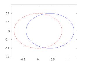
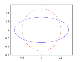
Figure 6.1: Two moving boundaries. Left: An ellipse moving with constant speed. Right: a circle morphing into an ellipse. Red dashed line: initial position; blue solid line: final position.

We illustrate the performance of our method in two moving geometries (Figure 6.1):

1. an ellipse moving with constant speed

   (6.1) $$\left\{\begin{aligned} y_{1}(\theta,t)&=0.8\cos(\theta)+0.4t,\\ y_{2}(\theta,t)&=0.2\sin(\theta),\end{aligned}\right.\qquad\theta\in[0,2\pi]$$

2. a circle deforming to an ellipse

   (6.2) $$\left\{\begin{aligned} y_{1}(\theta,t)&=(0.5+0.2t)\cos(\theta),\\ y_{2}(\theta,t)&=(0.5-0.2t)\sin(\theta),\end{aligned}\right.\qquad\theta\in[0,2\pi],\ 0\leq t\leq 1.$$

Example 1.

Validation of the asymptotic expansion Eq. 3.4 of the unsteady Stokes single layer potential.

To confirm the validity (and correctness) of the asymptotics for the single layer potential, we calculate the single layer potential on two moving boundaries for $t\in[0,T]$ with $T=0.075$ and density function

(6.3) $$\boldsymbol{\phi}(\mathbf{y},t)=\left(\cos(20y_{2}(\theta,T),3y_{1}^{3}(\theta,T)\right).$$

A 12-digit accurate reference solution is computed using our near-singular quadrature rules on the interval $[0,T-\epsilon_{M}]$ with 16$th$ order accurate spatial integration rules on a mesh with $200$ points. We then use the hybrid asymptotic/numerical method and compute the near-singular part on $[0,T-\epsilon]$ to 12-digit accuracy for various values of $\epsilon$. After adding the asymptotic contribution, this should match the reference solution with an error dominated by the asymptotics. Figure 6.2 shows the relative $l^{2}$ error as a function of $\epsilon$ for the two moving boundaries in Figure 6.1, which is clearly consistent with our analysis showing that it should be proportional to $\epsilon$.

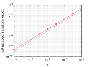
Figure 6.2: Asymptotic errors in the single layer potential Eq. 3.4. Red circles indicate numerical results and the dashed blue line is the function $y=10x$. Results for the moving boundary Eq. 6.1 are plotted on the left and results for the moving boundary Eq. 6.2 are plotted on the right.

Example 2.

Validation of the asymptotic expansion Eq. 3.12 of the unsteady Stokes double layer potential.

In our second experiment, we carry out the same analysis for the double layer potential, with the same strategy for validation. The results are shown in Figure 6.3, clearly showing the linear decrease of the error with $\epsilon$.

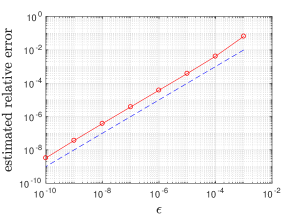
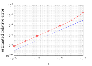
Figure 6.3: Asymptotic errors in the double layer potential Eq. 3.12. Red circles indicate numerical results and the dashed blue line is the function $y=10x$. Results for the moving boundary Eq. 6.1 are plotted on the left and results for the moving boundary Eq. 6.2 are plotted on the right.

Example 3.

Unsteady Stokes flow for a bounded, moving domain with velocity boundary conditions.

In our last example, we demonstrate the overall convergence of the full scheme for unsteady Stokes flow in a moving geometry, solving the integral equation Eq. 2.14 (in the absence of a forcing term). We use a scheme that is fourth order accurate in time and $16$th order in space, with an exact solution of the form

(6.4) $${\bf u}(\mathbf{x},t) =\sum_{j=1}^{5}\frac{1}{t^{2}}e^{-|\mathbf{x}-\mathbf{y}_{j}|^{2}/(4t)}\left(x_{2}-y_{j2},-(x_{1}-y_{j1})\right)$$

$$\quad+e^{-1/t}\sin(20t)e^{x_{1}}\left(\cos(x_{2}),-\sin(x_{2})\right),$$

where ${\bf x}=(x_{1},x_{2})$ and the $\{\mathbf{y}_{j}\}$ are chosen to be equispaced on the circle of radius $2$ centered at the origin, which encloses both domains of interest. The number of spatial discretization points is $200$ and the spatial discretization error is negligible. We place $100$ test points inside the computational domain. Table 6.1 lists the numerical results for both moving boundaries. Here $N$ is the total number of time steps, $\Delta t$ is the step size, $E$ is the relative $l^{2}$ error at the final time $T=1$, and $r$ is the ratio of relative $l^{2}$ errors for successive time step refinements. That is, $r(j)=E(j-1)/E(j)$, which gives a rough estimate of the convergence order. Note that $r\approx 2^{4}$, consistent with fourth order convergence once $\Delta t$ is sufficiently small.

Table 6.1: Numerical results for solving the problem of unsteady Stokes flow with velocity boundary conditions in the moving geometries shown in Figure 6.1.

$N$	$20$	$40$	$80$	$160$	$320$	$640$
$\Delta t$	$1/20$	$1/40$	$1/80$	$1/160$	$1/320$	$1/640$
Moving boundary Eq. 6.1
E	$5.6\cdot 10^{-5}$	$5.3\cdot 10^{-7}$	$1.7\cdot 10^{-7}$	$9.9\cdot 10^{-9}$	$5.8\cdot 10^{-10}$	$3.8\cdot 10^{-11}$
r		$107$	$3.0$	$17.5$	$17.2$	$15.4$
Moving boundary Eq. 6.2
E	$4.7\cdot 10^{-5}$	$3.6\cdot 10^{-7}$	$1.6\cdot 10^{-7}$	$9.8\cdot 10^{-9}$	$6.0\cdot 10^{-10}$	$3.8\cdot 10^{-11}$
r		$130$	$2.3$	$16$	$16$	$15.8$

7 Conclusions

We have developed a new method for the accurate evaluation of unsteady Stokes layer potentials in moving geometries. The scheme is based on splitting the local parts of the layer potentials into asymptotic and nearly-singular components. The leading order asymptotic contributions are derived analytically and the nearly-singular parts are handled accurately via a single Gauss-Legendre quadrature panel using an exponential change of variables in time. Numerical experiments demonstrate that the scheme converges at the expected rate for flows in bounded domains with velocity boundary conditions. One limitation of the current scheme is that the history part is handled using a spectral approximation of the Green’s function [9, 10, 21]. We are currently working on a marching scheme that represents the history part on an adaptive spatial mesh using the “bootstrapping” method of [27].

It is worth noting that the recently developed mixed potential method for unsteady Stokes flow [8] also permits high order accurate marching schemes in moving geometries. An advantage of that method is that it requires only harmonic and layer potentials, simplifying the fast algorithm and quadrature issues. A disadvantage is that it requires computation of the Helmholtz decomposition of the volume forcing term. Unsteady Stokes potentials lead to better-conditioned integral equations when using fully implicit marching schemes (at least for large time steps) and require only integration of the volume forcing term against the Green’s function. We intend to explore the relative performance of these two approaches in future work.

References

- [1] B. K. Alpert. Hybrid Gauss-trapezoidal quadrature rules. SIAM J. Sci. Comput., 20(5):1551–1584, 1999.
- [2] U. M. Ascher, S. J. Ruuth, and B. M. Wetton. Implicit-explicit methods for time-dependent partial differential equations. SIAM J. Numer. Anal., 32:797–823, 1995.
- [3] J. Bremer, Z. Gimbutas, and V. Rokhlin. A nonlinear optimization procedure for generalized Gaussian quadratures. SIAM J. Sci. Comput., 32(4):1761–1788, 2010.
- [4] D. L. Brown, R. Cortez, and M. L. Minion. Accurate projection methods for the incompressible Navier-Stokes equations. J. Comput. Phys., 168(2):464–499, 2001.
- [5] A. J. Chorin. Numerical solution of the Navier-Stokes equations. Math. Comput., 22:745–762, 1968.
- [6] E. B. Fabes, J. E. Lewis, and N. M. Riviere. Boundary value problems for the Navier-Stokes equations. Am. J. Math., 99:626–668, 1977.
- [7] E. B. Fabes, J. E. Lewis, and N. M. Riviere. Singular integrals and hydrodynamic potentials. Am. J. Math., 99:601–625, 1977.
- [8] L. Greengard and S. Jiang. A new mixed potential representation for the equations of unsteady, incompressible flow. arXiv:1809.08442, 2018.
- [9] L. Greengard and P. Lin. Spectral approximation of the free-space heat kernel. Appl. Comput. Harmon. Anal., 9:83–97, 2000.
- [10] L. Greengard and J. Strain. A fast algorithm for the evaluation of heat potentials. Comm. Pure Appl. Math., 43:949–963, 1990.
- [11] R. B. Guenther and E. A. Thomann. Fundamental solutions of Stokes and Oseen problem in two spatial dimensions. J. Math. Fluid Mech., 9:489–505, 2007.
- [12] J. Helsing. A fast and stable solver for singular integral equations on piecewise smooth curves. SIAM J. Sci. Comput., 33(1):153–174, 2011.
- [13] J. Helsing and R. Ojala. Corner singularities for elliptic problems: integral equations, graded meshes, quadrature, and compressed inverse preconditioning. J. Comput. Phys., 227(20):8820–8840, 2008.
- [14] W. D. Henshaw. A fourth-order accurate method for the incompressible Navier-Stokes equations on overlapping grids. J. Comput. Phys., 113:13–25, 1994.
- [15] S. Jiang, S. Veerapaneni, and L. Greengard. Integral equation methods for unsteady Stokes flow in two dimensions. SIAM J. Sci. Comput., 34(4):A2197–A2219, 2012.
- [16] G. E. Karniadakis, A. Beskok, and N. Aluru. Microflows and Nanoflows. Springer, New York, 2005.
- [17] S. Kim and S. J. Karrila. Microhydrodynamics: Principles and Selected Applications. Dover, New York, 2005.
- [18] P. Kolm and V. Rokhlin. Numerical quadratures for singular and hypersingular integrals. Comput. Math. Appl., 41(3–4):327–352, 2001.
- [19] R. Kress. Linear Integral Equations, volume 82 of Applied Mathematical Sciences. Springer–Verlag, Berlin, third edition, 2014.
- [20] J. Li and L. Greengard. High order accurate methods for the evaluation of layer heat potentials. SIAM J. Sci. Comput., 31:3847–3860, 2009.
- [21] P. Lin. On the Numerical Solution of the Heat Equation in Unbounded Domains. PhD thesis, Courant Institute of Mathematical Sciences, New York University, New York, 1993.
- [22] J.-G. Liu, J. Liu, and R. L. Pego. Stable and accurate pressure approximation for unsteady incompressible viscous flow. J. Comput. Phys., 229(9):3428–3453, 2010.
- [23] J. Ma, V. Rokhlin, and S. Wandzura. Generalized Gaussian quadrature rules for systems of arbitrary functions. SIAM J. Numer. Anal., 33(3):971–996, 1996.
- [24] Y. Saad and M. H. Schultz. GMRES: a generalized minimal residual algorithm for solving nonsymmetric linear systems. SIAM J. Sci. Statist. Comput., 7(3):856–869, 1986.
- [25] Z. Shen. Boundary value problems for parabolic Lamé systems and a nonstationary linearized system of Navier-Stokes equations in Lipschitz cylinders. Am. J. Math., 113:293–373, 1991.
- [26] R. Temam. Sur l’approximation de la solution des equations de Navier-Stokes par la methode des fractionnarires II. Arch. Rational Mech. Anal., 33:377–385, 1969.
- [27] J. Wang. Integral equation methods for the heat equation in moving geometry. PhD thesis, Courant Institute of Mathematical Sciences, New York University, New York, September 2017.
- [28] J. Wang and L. Greengard. Hybrid asymptotic/numerical methods for the evaluation of layer heat potentials in two dimensions. Adv. Comput. Math., accepted, 2018.
- [29] N. Yarvin and V. Rokhlin. Generalized Gaussian quadratures and singular value decompositions of integral operators. SIAM J. Sci. Comput., 20(2):699–718, 1998.