Bound and unbound rovibrational states of the methane-argon dimer

Abstract

Peculiarities of the intermolecular rovibrational quantum dynamics of the methane-argon complex are studied using a new, ab initio potential energy surface [Y. N. Kalugina, S. E. Lokshtanov, V. N. Cherepanov, and A. A. Vigasin, J. Chem. Phys. 144, 054304 (2016)], variational rovibrational computations, and detailed symmetry considerations within the molecular symmetry group of this floppy complex as well as within the point groups corresponding to the local minimum structures. The computed (ro)vibrational states up to and beyond the dissociation asymptote are characterized using two limiting models: the rigidly rotating molecule’s model and the coupled-rotor model of the rigidly rotating methane and an argon atom orbiting around it.

I Introduction

Methane is an abundant molecule not only on Earth, but in the Universe Kalugina et al. (2016); Liu and Jäger (2004). On Earth it has the third largest contribution to the greenhouse effect, after water vapor and carbon-dioxide, meanwhile on Titan, the moon of Saturn it is the most important greenhouse gas Samuelson et al. (1997). Therefore, the interaction of methane with other simple molecules is of interest for astrochemistry and for atmospheric chemistry. There are several experimental and theoretical results for such systems including methane-water, CH${}_{4}\cdot$H₂O Sarka et al. (2016, 2017), methane-fluoride, CH${}_{4}\cdot$F^-, Fábri et al. (2013), and the mehane dimer, CH${}_{4}\cdot$CH₄ Buryak et al. (2013).

The first measurements for the methane-argon gas mixture at several temperatures were reported by Dore and Filabozzi Dore and Filabozzi (1990). The infrared spectrum was reported first by McKellar et al. in 1994 McKellar (1994), then Pak et al. measured the high-resolution spectra of CH${}_{4}\cdot$Ar and CH${}_{4}\cdot$Kr complexes in the 7 $\mu$m region. Later on, further high-resolution measurements and ab initio computations were performed for the CH${}_{4}\cdot$Ar system Wangler et al. (2003); Liu and Jäger (2004).

In spite of repeated attempts, the spectral lines within the bound region of the complex have remained elusive to experimentalists due to the very low induced dipole moment of the complex dominated by dispersion interactions (both isolated methane and isolated argon are apolar). This region is however well accessible to theoretical investigations due to the low dimensionality (3D) of the intermolecular degrees of freedom and the excellent rigid-monomer approximation. On the contrary, the experimentally well-accessible transitions to predissociative states of the complex are extremely challenging for theory due to the high-dimensionality (12D) of the six-atomic methane-argon system. A rigorous full-dimensional rovibrational study has not been completed, and full-dimensional, ab initio potential energy surface have not been developed yet. At the same time, the energy and lifetime of predissociative states carry ample information on the fine details of the inter- and intra-molecular quantum dynamics taking place under the influence of weak (here: dispersion) interactions. Due to the very weakly bound nature of this complex and the high-order symmetry of the methane molecule, it has been anticipated that kinetic couplings play an important role in its intermolecular and predissociative dynamics.

In the present work we take the opportunity to use a new, ab initio atom-molecule interaction potential energy surface of this dimer Kalugina et al. (2016) to study peculiarities of the rovibrational dynamics and related symmetry considerations.

II Computational details

Intermolecular potential energy surface

We use the three–dimensional potential energy surface (PES) determined by Kalugina et al. by ab initio computations at the CCSD(T)/CBS level of theory, and by fitting an analytical functional form to the data points Kalugina et al. (2016). The ab initio computations were carried out with a regular tetrahedral methane structure with $r_{\text{CH}}=2.06735$ bohr. There are two non–equivalent minima on this PES: the argon atom is in a face configuration at the global minimum (GM) structure corresponding to an $R=6.95$ bohr carbon-argon distance, and in an edge configuration with a larger $R=7.34$ bohr value at the secondary minimum (SM) structure. The saddle point connecting the two non-equivalent minima is located at the vertex position of the argon atom (Fig. 1). The dissociation energy ($D_{e}$) of the complex from the global minimum is 141.47 cm^-1 and it is 115.06 cm^-1 from the secondary minimum.

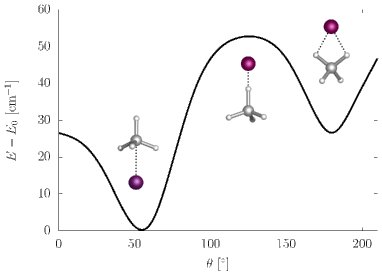
Figure 1: Angular dependence of the potential energy surface of Ref. Kalugina et al. (2016) represented in terms of $(R,\theta,\phi)$ spherical polar coordinates. For each $\theta$ value in the plot the $R$ coordinate was chosen to minimize the interaction energy, while $\phi$ was set to 0.0^∘.

Rovibrational computations

We carried out rovibrational computation on this intermolecular PES using the GENIUSH program Mátyus et al. (2009); Fábri et al. (2011). GENIUSH stands for GENeral Internal-coordinate, USer-define Hamiltonians, and it has been successfully used for the computation of bound and resonance states of floppy molecular systems, including ArNO⁺ Papp et al. (2017a), HeH${}_{2}^{+}$ Papp et al. (2017b), NH₃ Mátyus et al. (2009); Fábri et al. (2011), H${}_{5}^{+}$ Fábri et al. (2014), CH${}_{5}^{+}$ Fábri et al. (2017), CH${}_{4}\cdot$H₂O Sarka et al. (2017, 2016), with various internal coordinate and frame definitions. An interesting feature, the existence of formally negative-energy rotational excitations Wang and Jr. (2016); Schmiedt et al. (2015); Wodraszka and Manthe (2015); Fábri et al. (2014); Sarka et al. (2017, 2016) had been observed in a growing number of floppy systems and led to the introduction of the notion astructural molecules in Ref. Fábri et al. (2014). Ref. Fábri et al. (2014) also presented a one-dimensional torsional model to better highlight the phenomenon. Ref. Sarka et al. (2016) reported an elaborate study on the quantum dynamical background of these special features for the example of the methane-water dimer using a quantum mechanical, coupled-rotor model of the subsystems.

The general rovibrational Hamiltonian implemented in GENIUSH is

$$\begin{split}\hat{H}&=\frac{1}{2}\sum_{kl=1}^{D}\tilde{g}^{-1/4}\hat{p}^{\dagger}_{k}G_{kl}\tilde{g}^{1/2}\hat{p}_{l}\tilde{g}^{-1/4}\\ &+\frac{1}{2}\sum_{k}^{D}\sum_{\alpha}^{3}\left(\hat{p}_{k}G_{k,D+\alpha}+G_{k,D+\alpha}\hat{p}_{k}\right)\hat{J}_{\alpha}\\ &+\frac{1}{2}\sum_{\alpha}^{3}G_{D+\alpha,D+\alpha}\hat{J}_{\alpha}^{2}\\ &+\frac{1}{2}\sum_{\alpha}^{3}\sum_{\beta>\alpha}^{3}G_{D+\alpha,D+\beta}\left(\hat{J}_{\alpha}\hat{J}_{\beta}+\hat{J}_{\beta}\hat{J}_{\alpha}\right)+V,\end{split}$$ (1)

where $\hat{p}_{k}=-i\partial/\partial q_{k}$ is a differential operator corresponding to the $q_{k}$ internal coordinate, and $\hat{J}_{\alpha}$ ($\alpha=x,y,z$) labels the body-fixed angular momentum operators. The quantities $G_{kl}=(\boldsymbol{g}^{-1})_{kl}$ and $\tilde{g}=\text{det}(\boldsymbol{g})$ are obtained from the $g_{kl}$ mass-weighted metric tensor, defined as

$$g_{kl} =\sum_{i=1}^{N}m_{i}\textbf{t}_{ik}^{\text{T}}\textbf{t}_{il}, k,l\in\{1,2,...,D+3\}$$ (2)

$$\textbf{t}_{ik} =\frac{\partial\textbf{r}_{i}}{\partial q_{k}},$$ (3)

$$\textbf{t}_{D+\alpha} =\textbf{e}_{\alpha}\times\textbf{r}_{i},$$ (4)

which are evaluated over a direct product grid in the program using the user-defined body-fixed Cartesian coordinates in terms of the internal coordinates.

Geometrical constraints (in the present case for the methane molecule) are accounted for in an automated fashion by choosing $D$ being equal to the number of active vibrational dimensions ($D=3$ for the present case) in Eq. (1). This choice is equivalent to fixing the structural parameter (and a corresponding zero velocity) in the classical Lagrangian Mátyus et al. (2009). The Hamiltonian matrix is obtained as the matrix representation of Eq. (1) constructed with the discrete variable representation (DVR) for the vibrational degrees of freedom, and using the Wang functions for rotations. The kinetic energy operator is evaluated numerically over a direct product DVR grid. The eigenvalues and eigenfunctions of the Hamiltonian matrix are computed with an iterative Lanczos eigensolver.

We define the body-fixed Cartesian coordinates for the methane-argon complex, as follows: we place the carbon atom in the origin, two hydrogen atoms are in the $y-z$ plane and the other two are in the $x-y$ plane with the same methane geometry as the PES Kalugina et al. (2016). The position of the argon atom is defined by the $R,\cos\theta,$ and $\phi$ spherical polar coordinates, which are the active vibrational coordinates (for the basis functions, detailed intervals and DVR parameters see Table 1). The coordinate definition is completed by shifting the system to the center of mass of the complex. We used atomic masses Coursey et al. (2015), $m_{\text{H}}=1.007\ 825\ 032\ 23$ u, $m_{\text{D}}=2.014\ 101\ 778\ 12$ u, $m_{\text{T}}=3.016\ 049\ 277\ 9$ u, $m_{\text{C}}=12$ u, and $m_{\text{Ar}}=39.9623831237$ u, throughout the computations.

Table 1: Internal coordinate, basis function, number of DVR points ($N$), and grid intervals used in the computations.

Coordinate	Basis function	$N$	Grid interval
$R$ [Å]	Laguerre	51	[2.65–15]
$\cos\theta$	Legendre	81	Unscaled
$\phi$ [∘]	Fourier	21	[0–360)

III Symmetry considerations and analysis tools

This section is dedicated to a general description of the symmetry analysis and symmetry properties of the limiting (rigid-rotor and coupled-rotor) models, which will be used to understand the numerical results in Section IV.

III.1 Point groups and the molecular symmetry group of the methane-argon dimer

The PES of Ref. Kalugina et al. (2016) features two non-equivalent minima. The global minimum has a $C_{\text{3v}}$ point-group (PG) symmetry, while the secondary minimum has $C_{\text{2v}}$ PG symmetry (Figs. 1 and 2). With the low barriers and the almost freely rotating methane unit in the dimer, there is an interchange among the four GM and the six SM structures that gives rise to a rich splitting pattern.

The methane-argon dimer belongs to the $T_{\text{d}}$(M) molecular symmetry (MS) group and all symmetry species of the MS group are physically existing Bunker and Jensen (2006).

III.2 General considerations about the tunneling splitting of vibrational states

The splitting of vibrational states, classified by PG irreducible representation (irrep) labels, will be derived by starting out from a simple picture. Let us imagine that the system exhibits only small ($\varepsilon$) amplitude vibrations about the minimum structures (of one of the PG symmetries). This system is almost “frozen” at the near proximity of these equilibrium structures, and thus its molecular symmetry group is the permutation-inversion group isomorphic to the PG (with a selected numbering of the nuclei). Hence, these $\varepsilon$-vibrations can be characterized by irreps of the PG, $C_{\text{3v}}$(PG) or $C_{\text{2v}}$(PG), but they can also be characterized by the $C_{\text{3v}}$(M) and $C_{\text{2v}}$(M) permutation-inversion (PI) groups. These PI groups share elements with the MS group, which will be used later.

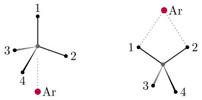
Figure 2: The global minimum has $C_{3\text{v}}$ point-group symmetry, whereas the local minimum has $C_{2\text{v}}$ point-group symmetry (this particular numbering of the nuclei is used in the derivation in the text).

For a general derivation of the vibrational splittings due to the large-amplitude motions, we proceed as follows. First, we construct the symmetry-adapted basis functions for the irreps of the PI group (isomorphic with the PG) of the minimum structure. Then, we consider the transformation properties of these functions under the symmetry operations of the MS group, determine the characters for each class of the MS group, and reduce the representation. We carry out the derivation for a general pair of MS and PI ($\sim$PG) groups, labelled with $G$ and $g$, respectively. At the end of the derivation, we calculate the splittings for the case of methane-argon.

1. Let us consider a function $f_{0}$ localized at an arbitrarily selected version of the molecule.

2. Map the $f_{0}$ basis function onto all feasible versions, $f_{i}=\hat{O}_{i}f_{0}$, by using all $\hat{O}_{i}$ $i\in\{1,2,\cdots,N\}$ MS group operations ($N=|G|$ is the order of $G$).

3. It is always possible to choose $f_{0}$ in such way that $\innerproduct{f_{i}}{f_{j}}=\delta_{ij}$ ($i,j=1,\ldots,N)$).

4. Construct a linear combination of the $f_{i}$ $(i=1,\ldots,N)$ functions which transform according to the $\mathit{\Gamma}$ irrep of $g$:

   $$\phi_{i}^{(\mathit{\Gamma})}=\frac{1}{n}\sum_{k=1}^{n}c_{k}^{(\mathit{\Gamma})}\hat{P}_{k}f_{i},\quad i=1,\ldots,N$$ (5)

   where $\hat{P}_{k}\in g$ and $n=|g|$ is the order of $g$.

5. In order to determine the characters in $G$, the trace of the matrix representation of $\hat{O}_{R}\in G$ is calculated corresponding to the $\{\phi_{i}^{(\mathit{\Gamma})};i=1,\ldots,N\}$ set of functions:

   $$\begin{split}\chi^{(\mathit{\Gamma})}(\hat{O}_{R})&=\sum_{i=1}^{N}\bra{\phi_{i}^{(\mathit{\Gamma})}}\hat{O}_{R}\ket{\phi_{i}^{(\mathit{\Gamma}})}\\ &=\frac{1}{n^{2}}\sum_{i=1}^{N}\sum_{k=1}^{n}\sum_{l=1}^{n}c_{k}^{(\mathit{\Gamma})}c_{l}^{(\mathit{\Gamma})*}\bra{\hat{P}_{k}f_{i}}\hat{O}_{R}\ket{\hat{P}_{l}f_{i}}\end{split}$$ (6)

6. In order to evaluate the trace in Eq. (6), we first identify the non-vanishing integrals by reordering the operators as

   $$\bra{\hat{P}_{k}f_{i}}\hat{O}_{R}\ket{\hat{P}_{l}f_{i}}=\bra{f_{i}}\hat{P}_{k}^{-1}\hat{O}_{R}\hat{P}_{l}\ket{f_{i}}.$$ (7)

   Since $g\subset G$ and due to the closure property of a group, $\hat{P}_{k}^{-1}\hat{O}_{R}\hat{P}_{l}\in G$. Since the set of (localized) $f_{i}$ functions was created by mapping $f_{0}$ with all possible operations of $G$, and the functions are orthogonal, a non-vanishing integral is obtained only if the product of the three operators, $\hat{P}_{k}^{-1}$, $\hat{O}_{R}$, and $\hat{P}_{l}$ equal the identity:

   $$\hat{P}_{k}^{-1}\hat{O}_{R}\hat{P}_{l}=\hat{I}$$ (8)

   $$\hat{O}_{R}=\hat{P}_{k}\hat{P}_{l}^{-1}.$$ (9)

7. The integral is non-vanishing for a selected $\hat{O}_{R}\in G$, if $\exists\hat{P}_{r}\in g$: $\hat{P}_{r}=\hat{O}_{R}$:

   $$\sum_{k=1}^{n}\sum_{l=1}^{n}\bra{f_{i}}\hat{P}_{k}^{-1}\hat{O}_{R}\hat{P}_{l}\ket{f_{i}}=n.$$ (10)

   Then, if $\mathit{\Gamma}$ is the totally symmetric irrep (assume that it is labelled with $\text{A}_{1}$) of $g$, all $c_{k}^{(\text{A}_{1})}$ characters equal 1, and we obtain:

   $$\chi^{\mathit{\Gamma}}(\hat{O}_{R}) =\frac{1}{n^{2}}\sum_{i=1}^{N}\sum_{k=1}^{n}\sum_{l=1}^{n}c_{k}^{\text{A}_{1}}c_{l}^{\text{A}_{1}}\bra{\hat{P}_{k}f_{i}}\hat{O}_{R}\ket{\hat{P}_{l}f_{i}}$$ (11)

   $$=\begin{cases}\frac{1}{n^{2}}Nn=\frac{N}{n},\text{\ if}\ \exists\ \hat{P}_{r}\in g:\hat{P}_{r}=\hat{O}_{R}\\ 0,\text{\ otherwise}\end{cases}$$ (12)

   For a different labeling of the atoms the $\hat{O}_{R}$ operators in the same class have different characters, thus we average over the $\chi(\hat{O}_{R})$ values within a class of the group. (Equivalently, we could have considered all possible labeling of the molecule at the beginning.) Let us denote the class of $\hat{O}_{R}$ as $\mathcal{R}$ and $K_{\mathcal{R}}$ is the number of elements in this class of $G$. Then, we obtain

   $$\chi^{\mathit{\Gamma}}(\mathcal{R}) =\frac{1}{K_{\mathcal{R}}}\sum_{\hat{O}_{R}\in\mathcal{R}}\chi(\hat{O}_{R})$$ (13)

   $$=\begin{cases}\frac{k_{r}}{K_{\mathcal{R}}}\frac{N}{n},\text{\ if}\ \exists\ \hat{P}_{r}\in g:\hat{P}_{r}=\hat{O}_{R}\in\mathcal{R}\\ 0,\text{\ otherwise,}\end{cases}$$ (14)

   and $k_{r}$ is the number of operations in the $\mathcal{R}$ class of $G$ for which $\exists\ \hat{P}_{r}\in g:\hat{P}_{r}=\hat{O}_{R}$. It can be seen that this $k_{r}$ number of operations equals the number of elements in the class of $g$ which contains $\hat{P}_{r}$.

8. In general for a $\mathit{\Gamma}$ irrep of $g$, the characters for the $\mathcal{R}$ class of $G$ are

   $$\chi^{(\mathit{\Gamma})}(\mathcal{R})=\begin{cases}c_{r}^{(\mathit{\Gamma})}\frac{k_{r}}{K_{\mathcal{R}}}\frac{N}{n},\text{\ if}\ \exists\ \hat{P}_{r}\in g:\hat{P}_{r}=\hat{O}_{R}\in\mathcal{R}\\ 0,\text{\ otherwise}.\end{cases}$$ (15)

III.3 Mathematical structure of the tunneling splittings in methane-argon

First, we calculate the tunneling splitting of the vibrational states for the global minimum structure. The order of $T_{\text{d}}(\text{M})$ is $N=24$. The global minimum (GM) has $C_{\text{3v}}$ PG symmetry, and the order of $C_{3\text{v}}$ (PG or PI) is $n=6$. The equivalent operations and the orders of classes in the two group are collected in Table 2.

Table 2: Equivalent operations in the $T_{\textnormal{d}}$(M) and $C_{3\text{v}}(\text{M})$ symmetry groups for the labeling shown in Fig. 2.

$T_{\textnormal{d}}$(M)	$E$	(123)	(14)(23)	[(1423)]*	[(23)]*
$K_{R}$	1	8	3	6	6
$C_{3\text{v}}$(M)	$E$	(123)			[(23)]*
$k_{r}$	1	2			3

The $T_{\text{d}}$(M) irreps for the vibrational splittings of states corresponding to the global minimum and the $C_{3\text{v}}$ PG (and its isomorphic MS) group are obtained from Eq. (15) and Table 2:

$$\begin{split}\mathit{\Gamma}_{\text{A}_{1}}^{C_{3\text{v}}}&=\textnormal{A}_{1}\oplus\textnormal{F}_{2}\\ \mathit{\Gamma}_{\text{A}_{2}}^{C_{3\text{v}}}&=\textnormal{A}_{2}\oplus\textnormal{F}_{1}\\ \mathit{\Gamma}_{\text{E}}^{C_{3\text{v}}}&=\textnormal{E}\oplus\textnormal{F}_{1}\oplus\textnormal{F}_{2},\end{split}$$ (16)

which defines the mathematical structure of the splitting pattern for the vibrational states assignable to the GM.

Table 3: Equivalent operations in the $T_{\textnormal{d}}$(M) and $C_{2\text{v}}(\text{M})$ symmetry groups for the labeling shown in Fig. 2.

$T_{\textnormal{d}}$(M)	$E$	(123)	(12)(34)	[(1234)]*	[(12)]*
$K_{R}$	1	8	3	6	6
$C_{3\text{v}}$(M)	$E$		(12)(34)		[(12)]*
$k_{r}$	1		1		1

We proceed similarly for the secondary minimum, use Eq. (15) and Table 3 for the $C_{\text{2v}}$ group (of order $n=4$), and obtain the splitting pattern for the vibrational states assignable to the SM as:

$$\begin{split}\mathit{\Gamma}_{\text{A}_{1}}^{C_{2\text{v}}}&=\text{A}_{1}\oplus\text{E}\oplus\text{F}_{2}\\ \mathit{\Gamma}_{\text{A}_{2}}^{C_{2\text{v}}}&=\text{A}_{2}\oplus\text{E}\oplus\text{F}_{1}\\ \mathit{\Gamma}_{\text{B}_{1}}^{C_{2\text{v}}}&=\text{F}_{1}\oplus\text{F}_{2}\\ \mathit{\Gamma}_{\text{B}_{2}}^{C_{2\text{v}}}&=\text{F}_{1}\oplus\text{F}_{2}.\end{split}$$ (17)

A difference in the mathematical structure of the GM and SM splittings is that the totally symmetric vibrations (such as the zero-point vibration) of the SM contain a doubly-degenerate species.

III.4 Coupled-rotor decomposition

Molecular systems which can be separated into two rigidly rotating distinct parts, can be characterized by a model which includes only the coupling of the subsystems’ angular momenta (and neglects any PES interactions). This scheme was introduced by Sarka et. al in relation with the general, numerical kinetic-energy operator approach of GENIUSH and is called the coupled-rotor decomposition (CRD) Sarka et al. (2017).

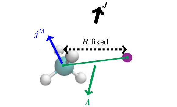
Figure 3: Coupling of the subsystems’ angular momenta used to define the coupled-rotor model in CH${}_{4}\cdot$Ar.

The coupled-rotor (CR) ansatz for methane-argon is constructed from the rotational wave functions of methane, $\phi_{km}^{j^{\text{M}}}$, and of the effective diatomic rotor, $Y_{\mathit{\Lambda}}^{m}$, coupled to a total rotational angular momentum state, $\ket{JM}$. Hence, the CR functions are defined as

$$[j^{\text{M}},\mathit{\Lambda}]_{JM}=\sum_{\mu}^{j^{\text{M}}}\sum_{(M-\mu)}^{\mathit{\Lambda}}\innerproduct{j^{\text{M}},\mu,\mathit{\Lambda},(M-\mu)}{JM}\phi_{\mu}^{j^{\text{M}}}Y_{\mathit{\Lambda}}^{M-\mu},$$ (18)

where $\innerproduct{j^{\text{M}},\mu,\mathit{\Lambda},(M-\mu)}{JM}$ are the Clebsch–Gordan coefficients. Based on this definition, the symmetry properties of the rotational functions, and the equivalent (monomer) rotations of the MS group operators, closed analytic expression can be derived for the symmetry labels of the CR functions. The characters and irrep decomposition in $T_{\text{d}}$(M) are given in Tables 4 and 5 for the $J=0$ and $J=1$ CR functions of methane-argon.

Table 4: Characters and irrep decomposition of the $J=0$ rotational functions of the methane-argon dimer in the $T_{\textnormal{d}}$(M) molecular symmetry group. $n_{\text{cl}}$ is the number of operations in the class.

	$E$	(123)	(14)(23)	[(1423)]*	[(23)]*
$n_{\textnormal{cl}}$	1	8	3	6	6
$\mathit{\Gamma}$						Irreps
$[0,0]_{00}$	1	1	1	1	1	A1
$[1,1]_{00}$	3	0	1	$-1$	1	F2
$[2,2]_{00}$	5	$-1$	1	$-1$	1	E $\oplus$ F2
$[3,3]_{00}$	7	1	$-1$	1	1	A1 $\oplus$ F1 $\oplus$ F2
$[4,4]_{00}$	9	0	1	1	1	A1 $\oplus$ E $\oplus$ F1 $\oplus$ F2
$[5,5]_{00}$	11	$-1$	$-1$	$-1$	1	E $\oplus$ F1 $\oplus$ F2
$[6,6]_{00}$	13	1	1	$-1$	1	A1 $\oplus$ A2 $\oplus$ E $\oplus$ F1 $\oplus$ 2 F2

Table 5: Characters and irrep decomposition of the $J=1$ rotational functions of the methane-argon dimer in the $T_{\textnormal{d}}$(M) molecular symmetry group.

	$E$	(123)	(14)(23)	[(1423)]*	[(23)]*
$n_{\textnormal{cl}}$	1	8	3	6	6
$\mathit{\Gamma}$						Irreps
$[0,1]_{10}$	1	1	1	$-1$	$-1$	A2
$[1,0]_{10}$	3	0	$-1$	1	$-1$	F1
$[1,1]_{10}$	3	0	$-1$	$-1$	1	F2
$[1,2]_{10}$	3	0	$-1$	1	$-1$	F1
$[2,1]_{10}$	5	$-1$	1	1	$-1$	E $\oplus$ F1
$[2,2]_{10}$	5	$-1$	1	$-1$	1	E $\oplus$ F2
$[2,3]_{10}$	5	$-1$	1	1	$-1$	E $\oplus$ F1
$[3,2]_{10}$	7	1	$-1$	$-1$	$-1$	A2 $\oplus$ F1 $\oplus$ F2
$[3,3]_{10}$	7	1	$-1$	1	1	A1 $\oplus$ F1 $\oplus$ F2
$[3,4]_{10}$	7	1	$-1$	$-1$	$-1$	A2 $\oplus$ F1 $\oplus$ F2
$[4,3]_{10}$	9	0	1	$-1$	$-1$	A2 $\oplus$ E $\oplus$ F1 $\oplus$ F2
$[4,4]_{10}$	9	0	1	1	1	A1 $\oplus$ E $\oplus$ F1 $\oplus$ F2
$[4,5]_{10}$	9	0	1	$-1$	$-1$	A2 $\oplus$ E $\oplus$ F1 $\oplus$ F2
$[5,4]_{10}$	11	$-1$	$-1$	1	$-1$	E $\oplus$ 2 F1 $\oplus$ F2
$[5,5]_{10}$	11	$-1$	$-1$	$-1$	1	E $\oplus$ F1 $\oplus$ 2 F2

In order to measure the similarity of the CR model and the “exact” intermolecular wave functions, we compute CRD overlaps defined as Sarka et al. (2017)

$$\text{CRD}^{J}_{nm}=\sum_{r=1}^{N_{R}}\absolutevalue{\sum_{k=-J}^{J}\sum_{i=1}^{N_{\Omega}}\tilde{\Psi}^{J}_{nk}(\rho_{r},\omega_{i})\tilde{\varphi}^{J}_{mk}(\omega_{i})}^{2}.$$ (19)

where $\tilde{\Psi}^{J}_{nk}(\rho_{r},\omega_{i})$ is the exact variational (ro)vibrational wave function in DVR, $\rho$ and $\omega$ denote the radial and (the collection of) angular coordinates respectively, and $\tilde{\varphi}^{J}_{mk}(\omega_{i})$ are the CR functions depending only on the angular coordinates. By identifying the dominant values in the CRD matrix the assignment of the (ro)vibrational states is straightforward.

In order to be able to numerically evaluate this integral in a “black-box fashion” of the GENIUSH protocol Mátyus et al. (2009), we compute the CR functions in a reduced-dimensionality GENIUSH computation with the atom-molecule distance fixed at its equilibrium value, the PES switched off, and the same angular grid representation as for the “full” problem (Table 1). The $T_{\text{d}}$(M) irrep labels are assigned to the (ro)vibrational states in an almost automated fashion by inspecting the numerical CRD matrix and using the symmetry properties of the CR functions (see Tables 4–5).

III.5 Rigid-rotor decomposition

In the traditional picture of molecular rotations and vibrations, molecular rotations Bunker and Jensen (2006); Wilson et al. (1980) are superimposed on the (higher-energy) molecular vibrations. The rigid-rotor decomposition (RRD) scheme was introduced Mátyus et al. (2010) to assign parent vibrational states to rovibrational wave functions. The RRD assignment is based on the overlap of a direct product basis of pure vibrational functions, $\psi^{J=0}_{n}$ and the $\phi^{\text{RR},J}$ rigid-rotor functions with the full rovibrational wave function, $\psi^{J>0}_{n}$ (computed with a selected body-fixed frame):

$$\ket{\psi^{J=0}_{n}}\otimes\ket{J,\phi^{\text{RR}}_{l}}=\ket{\psi^{J=0}_{n}\cdot\phi^{\text{RR},J}_{l}}$$ (20)

$$S_{nl,m}=\innerproduct{\psi^{J=0}_{n}\cdot\phi^{\text{RR},J}_{l}}{\psi^{J>0}_{m}}.$$ (21)

By computing the $S_{nl,m}$ overlap values, the dominant contribution of a vibrational state to a rovibrational state can be determined.

In the present work, besides the analysis of the numerical RRD values, we would like to better understand the regularities in the RRD matrix introduced by symmetry relations. First of all, we determine the symmetry assignment of the $\phi^{\text{RR},J}$ functions in the $T_{\text{d}}$(M) MS group. The equivalent rotations ($\alpha_{0},\beta_{0},\gamma_{0}$) for each class in the $T_{\text{d}}$(M) are (123): $\left(0,0,\frac{2\pi}{3}\right)$; (14)(23): $\left(\frac{\pi}{3},\pi,0\right)$; [(1423)]*: $\left(\frac{\pi}{6},\frac{\pi}{2},-\frac{\pi}{6}\right)$; [(23)]*: $\left(0,\pi,0\right)$. The characters of this reducible representation are the traces of Wigner $D$ matrices.

$$\chi^{j}=\sum_{m=-j}^{j}D^{j}_{m,m}(\alpha_{0},\beta_{0},\gamma_{0})$$ (22)

The irrep decompositions for several $J$ quantum numbers are collected in Table 6.

Table 6: Characters and irrep decomposition of the $\phi^{\text{RR},J}$ rigid-rotor functions in the $T_{\textnormal{d}}$(M) MS group.

	$E$	(123)	(14)(23)	[(1423)]*	[(23)]*
$n_{\textnormal{cl}}$	1	8	3	6	6
$\mathit{J}$						Irreps
0	1	1	1	1	1	A1
1	3	0	$-1$	1	$-1$	F1
2	5	$-1$	1	$-1$	1	E $\oplus$ F2
3	7	1	$-1$	$-1$	$-1$	A2 $\oplus$ F1 $\oplus$ F2
4	9	0	1	1	1	A1 $\oplus$ E $\oplus$ F1 $\oplus$ F2

Since the symmetry of the RRD basis functions, Eq. (20), is determined by the direct product of the $\mathit{\Gamma}(\psi^{J=0})$ and $\mathit{\Gamma}(\phi^{\text{RR},J>0})$ representations, the overlap in Eq. (21) can only be non-zero if the direct product contains the irrep of the rovibrational state. The irrep decomposition in $T_{\text{d}}$(M) of the direct product of the $\psi^{J=0}_{n}$ vibrational (A₁, A₂, E, F₁, F₂) and $\phi^{\text{RR},J>0}$, which is F₁ for $J=1$:

$$\begin{split}\text{A}_{1}\otimes\text{F}_{1}&=\text{F}_{1}\\ \text{A}_{2}\otimes\text{F}_{1}&=\text{F}_{2}\\ \text{E}\otimes\text{F}_{1}&=\text{F}_{1}\oplus\text{F}_{2}\\ \text{F}_{1}\otimes\text{F}_{1}&=\text{A}_{1}\oplus\text{E}\oplus\text{F}_{1}\oplus\text{F}_{2}\\ \text{F}_{2}\otimes\text{F}_{1}&=\text{A}_{2}\oplus\text{E}\oplus\text{F}_{1}\oplus\text{F}_{2}.\end{split}$$ (23)

This result tells us, for example, that a rovibrational state of A₂ symmetry can only originate from an F₂ vibrational state.

IV Numerical results

IV.1 Vibrational states

The depth of the PES valley of the global (secondary) minimum measured from the dissociation asymptote is $-D_{e}(\text{GM})=-141.47$ cm^-1 ($-D_{e}(\text{SM})=-115.06$ cm^-1). By considering also the zero-point vibration (ZPV) of the GM, the lowest-energy state accessible to the system has an energy $-D_{0}=-D_{e}+\text{ZPVE}=-88.60$ cm^-1, measured from the dissociation asymptote. The PES bounds 20 vibrational states (if we count degenerate states only once), which have been assigned using the limiting models described in Sec. III. The computed energy levels, together with their CRD and $T_{\text{d}}$(M) irrep assignments, are collected in Table 7 (see also Figure 4).

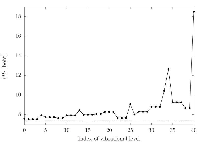
Figure 5: Expectation value of the carbon-argon distance, $R$, for the bound vibrational states of CH${}_{4}\cdot$Ar.

First of all, by looking at the computed and assigned list of vibrational states, we have attempted to identify complete splitting patterns, which (would) correspond to the traditional picture of molecular vibrations split up by feasible interchanges between the permutation-inversion versions. Having in mind the mathematical structure of the splittings for GM and SM vibrations, Eqs. (16) and (17), we have inspected the expectation value of the atom-molecule separation over the bound vibrational states (Fig. 5). Due to the structural differences between GM and SM ($R_{\text{eq}}(\text{GM})=6.95$ bohr and $R_{\text{eq}}(\text{SM})=7.34\ a_{0}$, respectively), an increased atom-molecule separation can be an indication of a secondary-minimum character. Alternatively, an increased $\langle R\rangle$ value can also indicate vibrational excitation along the atom-molecule distance. Stretching vibrational excitations and overtones can be recognized by nodes in the wave function along the $R$ coordinate. Figure 6 collects cuts of A₁-symmetry wave functions which highlight their nodal structure along $R$ (the Supplementary Material contains similar cuts for the bound vibrational states).

In addition, we repeated the vibrational computation also for the two symmetrically substituted isotopologues, CD${}_{4}\cdot$Ar and CT${}_{4}\cdot$Ar (Fig. 7). According to chemical-physical intuition, we expected that the tunneling splittings should get smaller by increasing the mass of the nuclei, which then could help the identification of the vibrational splittings.

Based on all these considerations and the numerical results, the zero-point vibration of the global minimum, ZPV(GM), could be assigned to J0.1 (0.00 cm^-1, A₁) and J0.2–4 (9.01 cm^-1, F₂). The next six states, J0.5 (28.74 cm^-1, A₁), J0.6–8 (31.24 cm^-1, F₂), and J0.9–10 (32.08 cm^-1, E) could be assigned to the zero-point vibration of the secondary minimum, ZPV(SM), but due to a node along the $R$ coordinate it would be morea appropriate to assign J0.5 (28.74 cm^-1, A₁) and J0.6–8 (31.24 cm^-1, F₂) to the intermolecular vibrational fundamental of the global minimum, Stre(GM). In general, the overlap of the energy range of the ZPV(SM) and Stre(GM) (and other vibrations), and the appearance of the same symmetry species in the different splittings, Eqs. (16) and (17), an unambiguous identification of vibrational states (in the traditional sense, split up by feasible exchanges) is hardly possible.

Furthermore, the higher the energy, the number of nodes along $R$ is less obvious (Fig. 6). While, we can trace (the A₁ species of) the first, second, and perhaps also the third stretching excitations by node counting, beyond J0.26 (68.90 cm^-1, A₁), the wave functions along $R$ become more and more oscillatory indicating that we approach the dissociation limit.

It is interesting to note that there is not any bound vibrational state of A₂ symmetry, which would be an “indicator” of a vibrational state of A₂(GM) or an A₂(SM) PG symmetry, Eqs. (16) and (17). Table IV shows that the lowest-energy CR-functions, which generate an A₂-symmetry state belong to $[6,6]_{00}$. These CR functions have $\sim$210 cm^-1 energy, much larger than the dissociation energy, which explains the absence of bound states of A₂ symmetry.

While it is difficult to use the traditional picture of molecular vibrations, the CR model appears to be useful and we could identify dominant CR functions for all vibrational states of methane-argon (see Figure 4 and Table 7).

Upon isotopic substitution, we could not really observe the closure of the splittings (since there are not any clear splittings apart from ZPV(GM)), but we observed another regularity with respect to the increase of the hydrogenic mass. Based on this regularity, we will explain the change in the energy ordering of the symmetry species along the CH${}_{4}\cdot$Ar–CD${}_{4}\cdot$Ar–CT${}_{4}\cdot$Ar sequence (Fig. 7).

The rotational constant, and thus the rotational energy of methane is inversely proportional to the mass of the H (D/T) atom, and thus the energy of the $[j^{\text{M}},\Lambda]_{00}$ CR functions is also proportional to $m_{\text{H}}^{-1}$ to a good approximation (we neglect the energetic contribution from the diatom rotation, which is small). If we check the energy separation of the lowest-energy vibrational states dominated by the $[0,0]_{00}$ (A₁), $[1,1]_{00}$ (F₂), $[2,2]_{00}$ (E$\oplus$F₂), and $[3,3]_{00}$ (A${}_{1}\oplus$F${}_{1}\oplus$F₂) CR functions, we observe a ca. 1/2 and 1/3 reduction in the energy separation (indicated with double-headed arrows in Fig. 7) upon the H–D and H–T replacement, respectively. Of course, the changes in the vibrational energy intervals only approximately follow the CR model, because the PES also has a role in the vibrational dynamics.

In comparison with the $m_{\text{H}}^{-1}$ relation of the CR splittings, the energy of the atom-molecule stretching excitations (excitation along $R$) changes approximately with $1/\sqrt{\mu}$, the square root of the reduced mass of the effective diatom (methane and argon), which brings in a less than a $1/\sqrt{2}$ and $1/\sqrt{3}$ factor upon the H-D and H-T replacements, respectively.

Hence, the energy separation of vibrational states corresponding to angular (CR) excitations (with similar radial parts) is decreased by a larger extent than the energy separation of radial ($R$-stretching) excitations upon isotopic substitution. Since radial excitation does not change the symmetry, while angular (CR) excitation does, we observe a rearrangement in the energy ordering of the various symmetry species in the deuterated and tritiated isotopologues.

Table 7: Bound-state vibrational energies given with respect to the $52.86$ cm^-1 zero-point vibrational energy of CH${}_{4}\cdot$Ar obtained with GENIUSH and the PES of Ref. Kalugina et al. (2016). Each vibrational state is characterized with its $T_{\textnormal{d}}$(M) irrep label ($\mathit{\Gamma}$) and the dominant (and minor) CR function.

n	$E$ [cm-1]	$\mathit{\Gamma}$	Coupled-rotor states    ($J=0$)
			dominant	minor
J0.1	52.86	A1	[0,0]00
J0.2–4	9.01	F2	[1,1]00
J0.5	28.74	A1	[0,0]00
J0.6–8	31.24	F2	[2,2]00	[1,1]00
J0.9–10	32.08	E	[2,2]00
J0.11–13	44.37	F2	[1,1]00	[2,2]00
J0.14	51.98	A1	[0,0]00
J0.15–17	55.78	F2	[2,2]00	[1,1]00 & [3,3]00
J0.18–19	63.73	E	[2,2]00
J0.20–22	65.53	F2	[1,1]00	[3,3]00
J0.23–25	65.81	F1	[3,3]00
J0.26	68.90	A1	[0,0]00	[3,3]00
J0.27	73.41	A1	[3,3]00	[0,0]00
J0.28–30	74.97	F2	[2,2]00	[1,1]00 & [3,3]00
J0.31–33	78.86	F2	[1,1]00	[2,2]00
J0.34	80.55	A1	[0,0]00
J0.35	86.25	A1	[0,0]00
J0.36–38	86.70	F2	[1,1]00	[2,2]00 & [1,1]00
J0.39–40	87.74	E	[2,2]00
J0.41	88.33	A1	[0,0]00

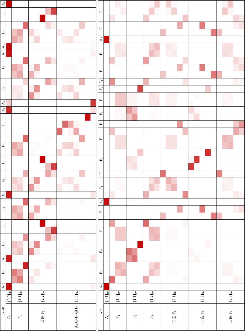
Figure 4: CRD overlap coefficients, Eq. (19), computed for the vibrational ($J=0$) and rovibrational ($J=1$) states of CH${}_{4}\cdot$Ar (a darker color corresponds to a larger value of the overlap). The rows correspond to the coupled-rotor functions $\varphi^{J}_{n}$, which are used to assign the full intermolecular vibrational states, $\Psi^{J}_{n}$, listed in the columns.

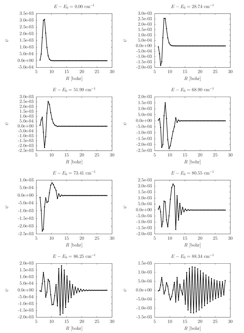
Figure 6: Wave function cuts along the $R$ coordinate for the A₁-symmetry vibrational states.

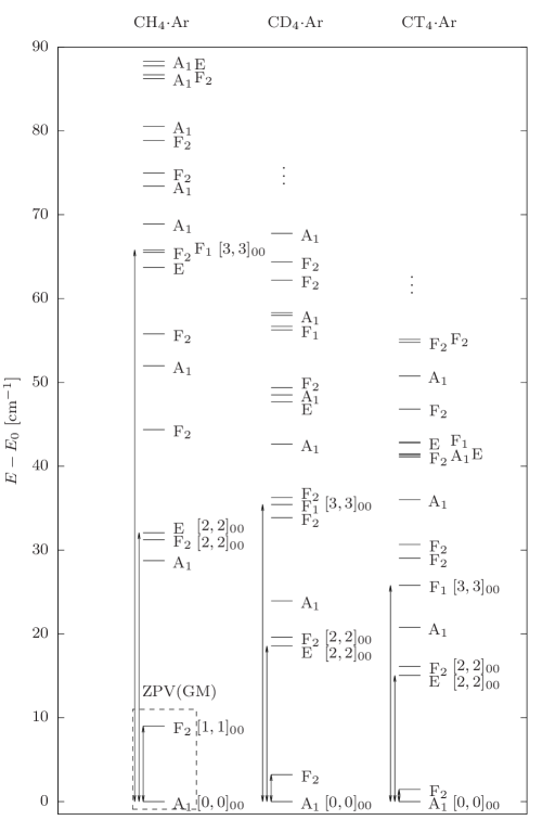
Figure 7: Comparison of the bound-state vibrational energies of CH${}_{4}\cdot$Ar, CD${}_{4}\cdot$Ar, and CT${}_{4}\cdot$Ar.

IV.2 Rovibrational states

The computed $J=1$ rovibrational results are summarized in Table 8. The corresponding CRD matrix is shown in Fig. 4, while the RRD coefficients (obtained with the RR functions corresponding to the symmetric-top GM structure) are visualized in Fig. 8. A clear assignment, of the vibrational parent (with dominant overlaps) is possible only for the lower-energy range. Nevertheless, we find it remarkable that it is possible to use the RR picture at all for this very floppy complex, in the light of the difficulties of identifying complete vibrational splitting manifolds (see previous section).

Surprisingly, the very first $J=1$ rotationally excited state (0.12 cm^-1, A₂) has a lower energy than its vibrational parent state (9.01 cm^-1, F₂) highlighted in Fig. 9. The rotational excitation of the ZPV(GM) (0.00 cm^-1, A₁) appears only as the second rotational state (9.07 cm^-1, F₁). This energy ordering of the rotational excitation of vibrational states is surprising if we have the traditional picture of rotating-vibrating molecules in mind. However, the traditional picture fails if the energy scale of rotations and intermolecular vibrations overlap which is the case for the present system.

Similarly to the vibrational states, the CR picture comes useful. The dominant CR functions in the lowest energy rotational state and in its parent vibration are the $[0,1]_{10}$ and $[1,1]_{00}$ functions, respectively. From this CR assignment, it can be seen that the unusual energy ordering is due to the rotational excitation of the methane unit which increases the energy but decreases the total rotational angular momentum, in the present case, due to its coupling with the rotating diatom. The opposite situation is observed for the second-lowest rotational state and its parent vibration, in which the $[1,0]_{10}$ and $[0,0]_{00}$ are the dominant CR functions, respectively. In this case, the rotational de-excitation of the methane molecule decreases the energy and (in this case) also the total rotational angular momentum is reduced. The symmetry pattern of the states follows the formal regularities derived for the RR functions, Eq. (23) (see also Fig. 8).

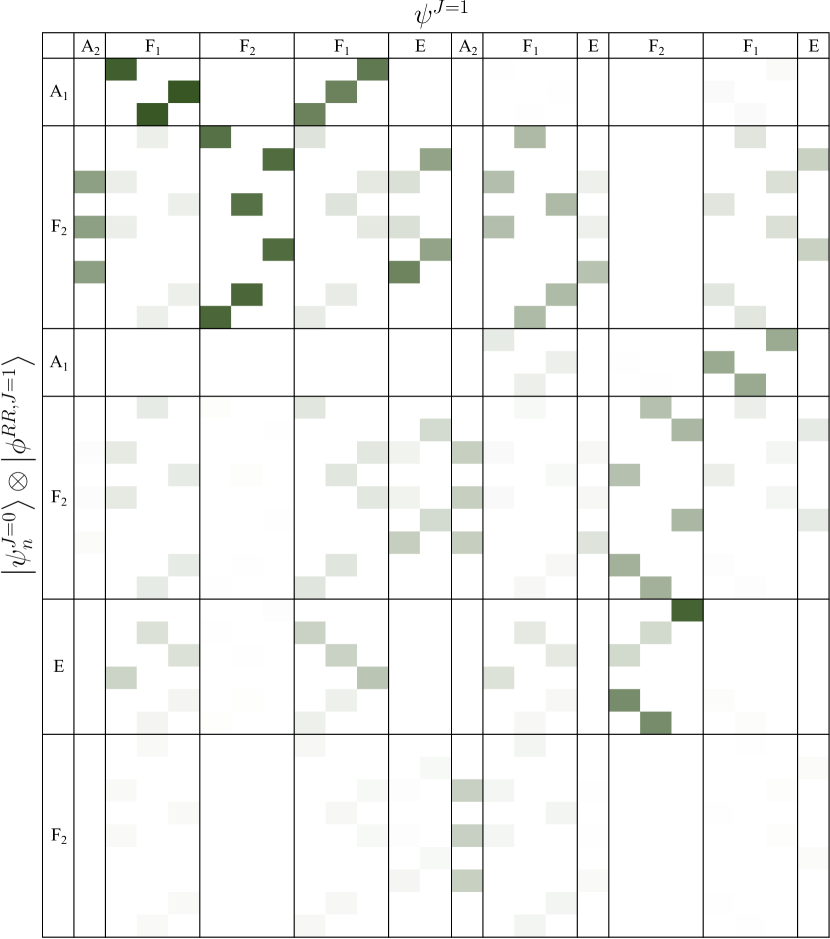
Figure 8: RRD overlap matrix, Eq. (21), for the $J=1$ rovibrational states of CH${}_{4}\cdot$Ar. The $\psi^{J=1}_{n}$ rovibrational functions listed in the columns are assigned with the product of the vibrational and rigid-rotor functions defined in Eq. (20).

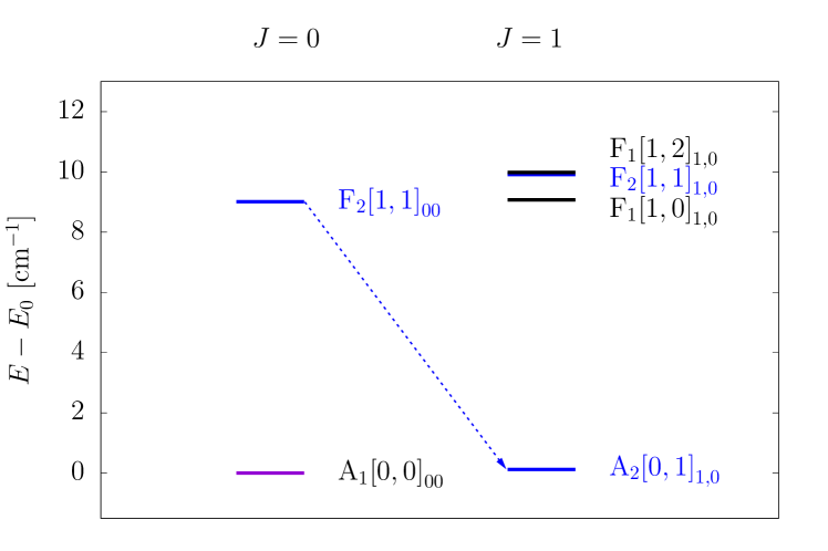
Figure 9: The lowest-energy $J=1$ rovibrational level of CH${}_{4}\cdot$Ar (0.12 cm^-1, A₂) has lower energy than its vibrational parent state, F₂ (9.01 cm^-1, F₂). The unusual energy ordering can be understood by inspecting the methane’s rotational excitation in the dominant CR functions, $[0,1]_{1,0}$ and $[1,1]_{0,0}$, respectively.

Table 8: Bound-state rovibrational energies ($J=1$), measured from the zero-point vibration energy, of CH${}_{4}\cdot$Ar obtained with GENIUSH and the PES of Ref. Kalugina et al. (2016). The assigned vibrational parent state, $T_{\textnormal{d}}$(M) irrep label ($\mathit{\Gamma}$), and the dominant (minor) coupled-rotor functions are also shown for each rovibrational state.

n	$E$ [cm-1]	Vib. parent	$\mathit{\Gamma}$	Coupled-rotor states    ($J=1$)
				dominant	minor
J1.0	0.12	F2 [9.01]	A2	[0,1]10
J1.1–3	9.07	A1 [0.00]	F1	[1,0]10	[1,2]10
J1.4–6	9.91	F2 [9.01] & E [32.08]	F2	[1,1]10
J1.7–9	9.98	A1 [0.00]	F1	[1,2]10	[1,0]10
J1.10–11	22.57	F2 [9.01] & F2 [31.24]	E	[2,2]10	[2,1]10 & [2,3]10
J1.12	28.86	F2 [31.24] & F2 [44.37]	A2	[0,1]10
J1.13–15	31.28	F2 [9.01]	F1	[2,1]10	[1,2]10
J1.16–17	31.93	F2 [9.01]	E	[2,1]10	[2,3]10
J1.18–20	31.94	E [32.08] & F2 [31.24]	F2	[2,2]10	[1,1]10
J1.21–23	32.01	A1 [28.74]	F1	[2,3]10	[1,0]10 & [2,1]10
J1.24–26	40.45	F2 [44.37]	F2	[1,1]10	[2,2]10
J1.27–29	40.46	A1 [28.74]	F1	[1,0]10	[1,2]10
J1.30–31	42.82	F2 [31.24]	E	[2,2]10	[2,1]10 & [2,3]10
J1.32–34	44.48	E [63.73]	F1	[1,2]10	[2,3]10 & [1,0]10
J1.35	52.08	F2 [55.78] & F2 [65.53]	A2	[0,1]10
J1.36–37	55.69	F2 [44.37]	E	[2,2]10	[2,1]10
J1.38–40	55.84	F2 [31.24]	F1	[2,3]10	[1,2]10 & [2,1]10
J1.41–43	58.32	F2 [55.78]	F2	[1,1]10	[2,2]10
J1.44–46	58.34	F1 [51.98]	F1	[1,0]10	[3,2]10 & [1,2]10
J1.47–48	63.58	F2 [44.37]	E	[2,3]10	[2,1]10
J1.49–51	65.55		F1	[1,2]10	[3,2]10
J1.52	65.78	F2 [31.24] & F2 [44.37]	A2	[3,2]10	[3,4]10
J1.53	65.83	F1 [65.81]	A1	[3,3]10
J1.54–56	65.91	F2 [65.53] & F1 [65.81]	F2	[1,1]10	[3,2]10
J1.57–59	66.03	A1 [51.98]	F1	[1,0]10	[3,4]10
J1.60–62	66.08	F2 [65.53]	F2	[3,4]10	[1,1]10
J1.63	68.99	F2 [78.86]	A2	[0,1]10
J1.64–65	71.49	F2 [55.78] & F2 [74.97]	E	[2,2]10	[2,3]10 & [2,1]10
J1.66	73.58	F2 [44.37]	A2	[3,4]10	[3,2]10 & [0,1]10
J1.67–69	74.33		F1	[3,3]10	[3,2]10 & [2,1]10
J1.70–72	74.42		F2	[3,2]10	[3,3]10 & [3,4]10
J1.73–75	75.12		F1	[2,3]10	[3,4]10
J1.76–78	78.95	A1 [68.90]	F1	[1,2]10	[1,0]10 & [2,3]10
J1.79–81	79.54	F2 [78.86]	F2	[1,1]10
J1.82–84	79.55	A1 [68.90]	F1	[1,0]10	[1,2]10
J1.85	80.60		A2	[0,1]10
J1.86–87	81.61	Several F2 states	E	[2,2]10	[2,1]10 & [2,3]10
J1.88	86.26		A2	[0,1]10
J1.89–91	86.69		F1	[1,2]10	[2,1]10 & [1,0]10
J1.92–94	87.31	F2 [86.70] & E [87.74]	F2	[2,2]10	[1,1]10
J1.95–97	87.34	A1 [80.55]	F1	[2,3]10	[2,1]10 & [1,0]10
J1.98–99	87.57	F2 [65.53]	E	[2,3]10	[2,1]10
J1.100	88.31		A2	[0,1]10

IV.3 Resonance states

Twenty vibrational bound states have been identified up to the dissociation asymptote (Table 7), and we continued the computations beyond the dissociation limit. Repeated computations with slightly different grid intervals of the molecule-atom distance allowed us to identify long-lived resonance states using the stabilization method Hazi and Taylor (1970) and a histogram analysis technique Papp et al. (2017a). Twenty GENIUSH computations were carried out, and 1000 eigenvalues were computed in each run with different box sizes. In every computation the maximal value for the $R$ coordinate was slightly modified, from 14.05 Å to 15 Å (the PES is defined up to $R=10$ Å), incremented by 0.05 Å in each computation. The computed eigenvalues are collected and sorted from the lowest to the largest, then a histogram is made from the data. The eigenvalues corresponding to the resonance states will appear in every computation, meanwhile the continuous eigenvalues are shifted by changing the size of the box. The obtained histogram (bin size 0.01 cm^-1) is shown in Figure 10 and the energy positions and assignment for the peaks are collected in Table 9.

It is interesting to note that we find only E and F₂-symmetry states among the identified long-lived resonances. The dominant CR functions in these states are $[1,1]_{00}$, $[2,2]_{00}$, and $[3,3]_{00}$. The lack of A₁ states may be explained by the fact that highly excited vibrations along the $R$ (dissociation) coordinate also have A₁ symmetry, and due to the coupling of states with the same symmetry, we do not observed any long-lived resonance of this species.

The absence of states dominated by the $[0,0]_{00}$ CR function tells us that a fair portion of the energy in these long-lived resonances appears in the angular degrees of freedom (the excitation of which is measured by the CRD). The presumably slow energy transfer from the angular degrees of freedom to the radial (dissociative) degree of freedom gives rise to a long lifetime of the identified states.

It is also insightful to compare the energy of the states with the dissociation energy $D_{0}(\text{GM})\approx 90$ cm^-1 (measured from the ZPV as in Fig. 10) and the CR energies of the $[n,n]_{00}$ functions with $n=1,2,$ and $3$: ca. 0 cm^-1, 10 cm^-1, 30 cm^-1, and 60 cm^-1, respectively. Assuming simple additivity of these energies, we may understand that long-lived states dominated by $[1,1]_{00}$ are possible up to ca. 100 cm^-1 (however, we do not have any simple explanation for the J0.73–75, F₂ state). Similarly, we may find long-lived states dominated by $[2,2]_{00}$ or $[3,3]_{00}$ up to ca. 130–140 cm^-1, which is indeed the case.

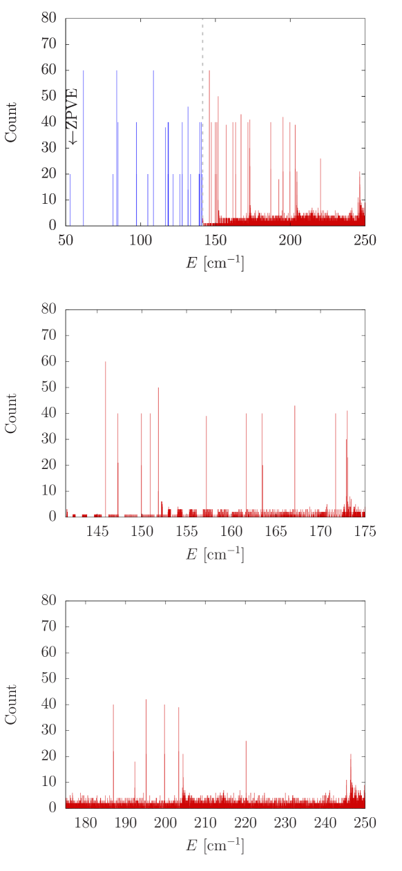
Figure 10: Bound (blue) and resonance (red) vibrational states of CH${}_{4}\cdot$Ar indicated by the peaks in the stabilization histogram. measured from the global minimum of the PES. (For some triply degenerate states an artificial split can be observed in the histogram due to imperfect convergence. An unambiguous symmetry assignment is established through a CRD analysis (see Table 9).)

All peaks above the $D_{e}$ dissociation energy (141.47 cm^-1) correspond to a resonance state (Fig. 10.). The symmetry assignment by CRD and the major and minor coupled rotor contributions are listed in Table 9.

Table 9: Energy of the long-lived ($J=0$) vibrational resonances of CH${}_{4}\cdot$Ar computed with GENIUSH, the PES of Ref. Kalugina et al. (2016), and the stabilization technique. The vibrational states are given with respect to the zero-point vibration energy. Each state is characterized with its $T_{\textnormal{d}}$(M) irrep label and the dominant (and minor) coupled-rotor functions.

n	$E$ [cm-1]	$\mathit{\Gamma}$	Coupled-rotor states    ($J=0$)
			dominant	minor
J0.42–44	93.06	F2	[1,1]00
J0.45–47	94.44	F2	[3,3]00	[2,2]00
J0.48–50	97.08	F2	[1,1]00	[2,2]00
J0.51–52	98.06	F2	[1,1]00	[2,2]00
J0.53–55	98.98	F2	[1,1]00
J0.56–57	104.36	E	[2,2]00
J0.58–59	108.82	E	[3,3]00
J0.60–62	110.60	F2	[3,3]00	[2,2]00
J0.63–64	114.25	E	[2,2]00
J0.65–66	118.82	E	[2,2]00
J0.67–68	120.03	E	[2,2]00
J0.69–70	134.08	E	[2,2]00	[3,3]00
J0.71–72	139.46	E	[3,3]00
J0.73–75	142.34	F2	[1,1]00	[2,2]00
J0.76–78	150.45	F2	[3,3]00	[2,2]00

V Summary

Rovibrational computations have been carried out for the methane-argon dimer using a new, ab initio atom-molecule potential energy surface Kalugina et al. (2016) and the general rovibrational program, GENIUSH Mátyus et al. (2009); Fábri et al. (2011). This PES, with a well depth of $-D_{\text{eq}}=-141.47$ cm^-1, supports twenty bound states (counting degenerate states only once). The energy of the lowest accessible vibrational state to the system is $-D_{0}(GM)=-88.60$ cm^-1, measured from the dissociation asymptote. Although there are two different minimum structures, with a 26.41 cm^-1 energy separation, most of the computed (ro)vibraitonal states cannot be unambiguously assigned either to the global or to the secondary minimum. The computed rovibrational states were analyzed using two limiting models and detailed symmetry considerations.

The traditional picture of molecular rotations and vibrations almost completely breaks down for this weakly bound, floppy system. We could identify the complete tunneling splitting only for the zero-point vibrational state of the global minimum. Vibrational parent states could be determined only for the lowest few rotational states with $J=1$ rotational quantum number. Interestingly, the lowest-energy rotational state does not correspond to the rotational excitation of lowest-energy vibrational state but it corresponds to the second lowest vibrational state. This rotational state and its vibrational parent represent a “formally” negative-energy rotational excitation, i.e., the rotationally excited state has a lower energy than its parent vibration.

These unusual features, which appear strange in terms of the traditional picture of rotating-vibrating molecules, can be well understood using a model which considers the rotating-vibrating complex in terms of coupled quantum rotors of rigidly rotating methane and the effective diatom (atom-molecule separation). All vibrational bound and low-energy, long-lived resonance states as well as most of the $J=1$ rovibrational states can be assigned within this coupled-rotor picture.

VI Acknowledgement

We thank Yulia Kalugina for sending to us the potential energy subroutine of methane-argon, and Gustavo Avila for initial discussions on this project. We acknowledge financial support from a PROMYS Grant (no. IZ11Z0_166525) of the Swiss National Science Foundation. F.D. also thanks the New National Excellence Program of the Ministry of Human Capacities of Hungary (ÚNKP-18-3-II-ELTE-133). A PRACE Preparatory Access Grant allowed us to test the applicability and scalability of the GENIUSH program on European Supercomputers (Barcelona, Paris, and Stuttgart), which is gratefully acknowledged.

References

- Kalugina et al. (2016) Y. N. Kalugina, S. E. Lokshtanov, V. N. Cherepanov, and A. A. Vigasin, J. Chem. Phys. 144, 054304 (2016).
- Liu and Jäger (2004) Y. Liu and W. Jäger, J. Chem. Phys. 120, 9047 (2004).
- Samuelson et al. (1997) R. E. Samuelson, N. R. Nath, and A. Borysow, Planetary and Space Science 45, 959 (1997), ISSN 0032-0633.
- Sarka et al. (2016) J. Sarka, A. G. Csaszar, S. C. Althorpe, D. J. Wales, and E. Matyus, Phys. Chem. Chem. Phys. 18, 22816 (2016).
- Sarka et al. (2017) J. Sarka, A. G. Csaszar, and E. Matyus, Phys. Chem. Chem. Phys. 19, 15335 (2017).
- Fábri et al. (2013) C. Fábri, A. G. Császár, and G. Czakó, J. Phys. Chem. A 117, 6975 (2013).
- Buryak et al. (2013) I. Buryak, Y. Kalugina, and A. Vigasin, J. Mol. Spectrosc. 291, 102 (2013).
- Dore and Filabozzi (1990) P. Dore and A. Filabozzi, Can. J. Phys. 68, 1196 (1990).
- McKellar (1994) A. R. W. McKellar, Faraday Discuss. 97, 69 (1994).
- Wangler et al. (2003) M. Wangler, D. Roth, I. Pak, G. Winnewisser, P. Wormer, and A. van der Avoird, J. Mol. Spectrosc. 222, 109 (2003).
- Mátyus et al. (2009) E. Mátyus, G. Czakó, and A. G. Császár, J. Chem. Phys. 130, 134112 (2009).
- Fábri et al. (2011) C. Fábri, E. Mátyus, and A. G. Császár, J. Chem. Phys. 134, 074105 (2011).
- Papp et al. (2017a) D. Papp, J. Sarka, T. Szidarovszky, A. G. Császár, E. Mátyus, M. Hochlaf, and T. Stoecklin, Phys. Chem. Chem. Phys. 19, 8152 (2017a).
- Papp et al. (2017b) D. Papp, T. Szidarovszky, and A. G. Császár, J. Chem. Phys. 147, 094106 (2017b).
- Fábri et al. (2014) C. Fábri, J. Sarka, and A. G. Császár, J. Chem. Phys. 140, 051101 (2014).
- Fábri et al. (2017) C. Fábri, M. Quack, and A. G. Császár, J. Chem. Phys. 147, 134101 (2017).
- Wang and Jr. (2016) X.-G. Wang and T. C. Jr., J. Chem. Phys. 144, 204304 (2016).
- Schmiedt et al. (2015) H. Schmiedt, S. Schlemmer, and P. Jensen, J. Chem. Phys. 143, 154302 (2015).
- Wodraszka and Manthe (2015) R. Wodraszka and U. Manthe, 6, 4229 (2015).
- Coursey et al. (2015) J. S. Coursey, D. J. Schwab, J. J. Tsai, and R. A. Dragoset, Atomic Weights and Isotopic Compositions (version 4.1): http://physics.nist.gov/Comp [last accessed on 12 May 2018]. National Institute of Standards and Technology, Gaithersburg, MD. (2015).
- Bunker and Jensen (2006) P. Bunker and P. Jensen, Molecular Symmetry and Spectroscopy (NRC Research Press, 2006).
- Wilson et al. (1980) E. B. Wilson, J. C. Decius, and P. C. Cross, Molecular Vibrations: the Theory of Infrared and Raman Vibrational Spectra (Courier Corporation, 1980).
- Mátyus et al. (2010) E. Mátyus, C. Fábri, T. Szidarovszky, G. Czakó, W. D. Allen, and A. G. Császár, J. Chem. Phys. 133, 034113 (2010).
- Hazi and Taylor (1970) A. U. Hazi and H. S. Taylor, Phys. Rev. A 1, 1109 (1970).