Spatially-selective in situ magnetometry of ultracold atomic clouds

Abstract

We demonstrate novel implementations of high-precision optical magnetometers which allow for spatially-selective and spatially-resolved in situ measurements using cold atomic clouds. These are realised by using shaped dispersive probe beams combined with spatially-resolved balanced homodyne detection. Two magnetometer sequences are discussed: a vectorial magnetometer, which yields sensitivities two orders of magnitude better compared to a previous realisation and a Larmor magnetometer capable of measuring absolute magnetic fields. We characterise the dependence of single-shot precision on the size of the analysed region for the vectorial magnetometer and provide a lower bound for the measurement precision of magnetic field gradients for the Larmor magnetometer. Finally, we give an outlook on how dynamic trapping potentials combined with selective probing can be used to realise enhanced quantum simulations in quantum gas microscopes.

I Introduction

Magnetometry has applications in a number of disciplines ranging from medicine to geophysics Budker and Derek F. Jackson Kimball (2013). High precision magnetometry also plays a central role in fundamental physics research, for instance in the search for a permanent electron electric dipole moment or signs of CPT violation Safronova et al. (2018).

State-of-the-art magnetometers are based on a variety of different methods. These prominently include superconducting quantum interference devices, solid state Hall sensors, magnetic resonance force microscopes, NV centres and optical magnetometers (OPMs) Budker and Derek F. Jackson Kimball (2013); [Seesupplementaryinformationof][.Thisgivesanexcellentsummaryoftheachievedsensitivitiesindifferentexperimentallyrealisedmagnetometersacrossthedifferentavailabletechnologies.]muessel_Scalable_2014.

OPMs are typically based on the interaction of a laser beam with polarised atomic media. In particular vapour-cell-based Spin-Exchange-Relaxation-Free (SERF) optical magnetometers offer the highest sensitivity to date Kominis et al. (2003); Dang et al. (2010). A special subgroup of OPMs are cold atom based magnetometers, which are at the focus of this work Vengalattore et al. (2007); Sewell et al. (2012). These devices have applications in laboratory based research, and their advantage lies in the combination of high sensitivity and high spatial resolution. This has been utilised for the detection of magnetic field gradients close to $100$ nG/$\mu$m Higbie et al. (2005); Koschorreck et al. (2011); Muessel et al. (2014b).

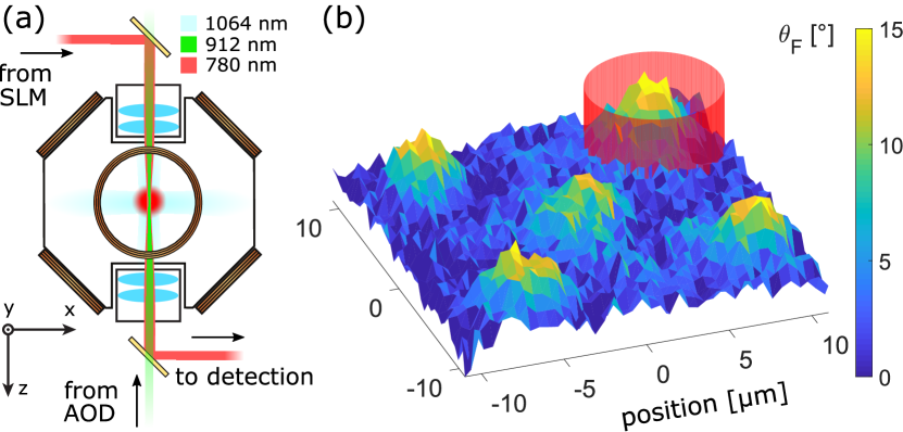
Figure 1: (a) Schematic of the optical setup and lasers used in our experiment. A detailed description is in the main text. (b) Our local dispersive probing scheme. The image is a raw dispersive image of the atomic distribution in a system of five microtraps. A red cylinder encircles one of five atomic clouds, as to illustrate how the vectorial dispersive imaging can be made to selectively probe a portion of the atomic system.

In a parallel development, spatial resolution and manipulation of ultra-cold atoms has been realised by employing spatial light modulators (SLMs) or acousto-optical deflectors (AODs) in order to create arbitrarily shaped light fields. AODs deflect a single laser beam depending on an applied radio frequency (RF) signal. More complex light patterns therefore need to be “painted” in a time-averaging approach Henderson et al. (2009), or by applying multi-tone RF signals Endres et al. (2016). AODs have not only been employed to transport Kaufman et al. (2015) and rearrange Barredo et al. (2016); Endres et al. (2016) single atoms in microtrap arrays but also in a multiplexed quantum memory module for writing and reading atomic states Pu et al. (2017). SLMs modify the phase and/or the amplitude of a laser beam spatially. Their usage in cold atom experiments has steadily been increasing since the first successful atom trapping with an SLM Bergamini et al. (2004), where the traps were generated by a phase modulation. Alternatively, potentials can be created by directly imaging the surface of an SLM onto atoms Brandt et al. (2011); Muldoon (2012). Recently, SLMs have been employed in quantum gas experiments to create ultra-low-entropy many-body quantum states Mazurenko et al. (2017). For a more extensive overview of the different implementations the interested reader is referred to Holland et al. (2018).

In this paper we describe techniques for spatially-selective and spatially-resolved, single-shot, in situ magnetometry with cold atoms. We discuss the operation of two types of magnetometers: First, a vectorial magnetometer which is capable of measuring the longitudinal field component along the probe beam direction, as well as the modulus of the two perpendicular field components in a single experimental realisation. This type of implementation offers good precision. Second, we realise a Larmor magnetometer which is sensitive to the modulus of the projection of the total field onto the probe axis and provides very high accuracy. Fig. 1 (a) shows the main features of the experiment. The atomic cloud is held in optical microtraps, generated with an AOD, and probed with dispersive light shaped with an SLM. The dual objective system in the apparatus allows for manipulation of the atomic cloud in optical tweezers, spatial shaping of the dispersive probe, and spatially-resolved detection of the atomic distribution.

Fig. 1 (b) depicts an array of five atomic clouds recorded in situ with dispersive imaging and shows the versatility of the microtrap setup. The spatial shaping of the dispersive probe beam opens the possibility of spatially-selective measurements of parts of the whole atomic system, as indicated by the red cylinder in Fig. 1 (b), leaving the other regions unaffected.

The dispersive nature of the measurement makes both magnetometer sequences applicable for in-sequence, in situ measurements of a shot-to-shot fluctuating magnetic field. Such fluctuations would otherwise be detrimental for any detailed investigation of quantum spin dynamics such as quantum simulations of spin-chains Simon et al. (2011). In the outlook we present our vision for how spatially-selective magnetic field detection in one portion of a system can enhance the precision of a magnetic field sensitive measurement in another part, in the context of a new quantum gas microscope experiment.

The structure of this paper is as follows. Sec. II presents the experimental setup, then Secs. III and IV describe the implementation of the two optical magnetometers. Finally Sec. V demonstrates the local nature of the dispersive measurement scheme.

II Experimental setup

The magnetometer sequences discussed here are based on atoms in optical dipole potentials. Our experimental setup was previously described in Bason et al. (2018) and the relevant steps are outlined below. An experimental cycle is initiated by collecting a cloud of ⁸⁷Rb atoms in a $3$D magneto-optical trap. It is subsequently optically pumped into the $\ket{F=2,m_{F}=2}$ state and magnetically transported to an intermediate vacuum chamber where forced microwave evaporation is performed Bason et al. (2018). Thereafter the cloud is loaded into a focused single beam optical dipole trap at a wavelength of $1064$ nm, with a $1/e^{2}$ waist of $45~{}\mu$m Heck et al. (2018). The cloud is then transported by moving the focus of the beam to a science chamber. Here, another laser beam, with a waist of $90~{}\mu$m, propagating at a right angle to the transport beam, forms a crossed dipole trap (CDT). Within the CDT we perform further evaporative cooling and obtain a thermal atomic cloud of about $2\cdot 10^{6}$ atoms at a temperature of $800$ nK.

The magnetic field at the position of the atoms is controlled by three orthogonal pairs of compensation coils as shown in Fig. 1 (a). Fast control of these coils is essential for the realisation of the magnetometer described below. The effect of $50$ Hz noise is minimised by triggering the sequence on the power line.

To allow for high-resolution imaging, the science chamber has two re-entrant viewports on opposing sides. They are equipped with objectives with an effective numerical aperture NA $=0.11$. One of the objectives is used to create optical potentials at high-resolution using laser light at $912$ nm (shown in Fig. 1 (a)). For flexible spatial control this light is sent through a two-axis AOD, enabling us to realise time-averaged potentials such as multiple, tightly focused beams. These optical tweezers have a waist of $4.3(1)~{}\mu$m leading to potential depths in individual tweezers of up to $100~{}\mu$K.

The dispersive light matter interaction can be decomposed to first order into scalar and vectorial components. The typical imaging techniques based on this interaction all have a similar signal-to-noise-ratio Gajdacz et al. (2013). Here we make use of the vectorial part that gives access to the magnetisation of the atomic cloud. This imaging technique is traditionally called Faraday imaging. It has commonly been measured with photodetectors, e.g. for magnetometry or spin-squeezing experiments Isayama et al. (1999); Sewell et al. (2012); Palacios et al. (2018), however these experiments lack the ability to obtain spatial information of the atomic clouds. Recently, spatially-resolved Faraday imaging has enabled studies of density effects in the light-matter interaction Kaminski et al. (2012), in situ dynamics of thermal atomic clouds Gajdacz et al. (2013), sub shot-noise atom number stabilised ultracold clouds Gajdacz et al. (2016) and the BEC phase transition itself Bason et al. (2018).

Here, we use the Faraday interaction to detect the atoms non-destructively. Briefly, a linearly polarised, off-resonant probe beam is sent through the atomic sample (shown in Fig. 1 (b)). Given that all atoms are prepared in the same internal state, the plane of polarisation of the probe is rotated by the Faraday angle $\theta_{F}$ according to $\theta_{F}(x,y)\sim\braket{f_{z}}\int\rho(x,y,z)\,dz$, where $\braket{f_{z}}$ is the average projection of the total angular momentum state per atom along the probing direction and $\rho(x,y,z)$ corresponds to the atom density Gajdacz et al. (2013); Bradley et al. (1997). In the limit of large atom numbers $\braket{f_{z}}$ can be treated as a classical quantity.

To achieve spatially-selective imaging, Faraday light is shaped by imaging the plane of a SLM (in our experiment a Digital Micromirror Device (DMD)) onto the atoms. After the chamber the Faraday light passes through a balanced homodyne polarimeter Kaminski et al. (2012). This polarimeter consists of a Wollaston prism which separates light into the horizontal and vertical polarisation components. These components are then imaged through the same imaging system onto separate areas of an electron multiplying charge-coupled device (EMCCD) camera (Andor iXon Ultra 897). The resulting images are denoted as $I_{\rm H}$ and $I_{\rm V}$, corresponding to the horizontal and vertical polarimeter ports, respectively. A Faraday image describes the spatially dependent angle $\theta_{F}$ and is generated by combining $I_{\rm H}$ and $I_{\rm V}$ according to Kaminski et al. (2012)

$$\theta_{F}=\frac{1}{2}\arcsin{\left(\frac{I_{\rm H}-I_{\rm V}}{I_{\rm H}+I_{\rm V}}\right)},$$ (1)

for each camera pixel. For optimal performance, careful polarisation balancing of $I_{\rm H}$ and $I_{\rm V}$ is crucial. In Fig. 2 (a) a raw image of the two polarisation fields is shown. Here the Faraday light is shaped as a flat top beam, but the light intensity varies somewhat due to imperfections in the imaging system. These variations will lead to increased technical noise in the Faraday image if $I_{\rm H}$ and $I_{\rm V}$ are not correctly centred with respect to each other. Using this noise as a measure allows one to find the right relative positioning of the images through a minimisation algorithm. Figs. 2 (b) and (c) are enlarged regions of the raw polarisation fields $I_{\rm V}$ and $I_{\rm H}$ around the position of the atoms. To account for remaining image artifacts originating in the optical setup, an averaged Faraday image without atoms (d) is subtracted. The final Faraday image in Fig. 2 (e) shows an atomic cloud trapped in a single optical tweezer, with a peak rotation angle of around $\theta_{F}\simeq 15^{\circ}$. The main advantage of minimally-destructive dispersive imaging methods is the option to take multiple images in a single realisation. This enables us to investigate dynamics in the atomic system Gajdacz et al. (2013); Bason et al. (2018).

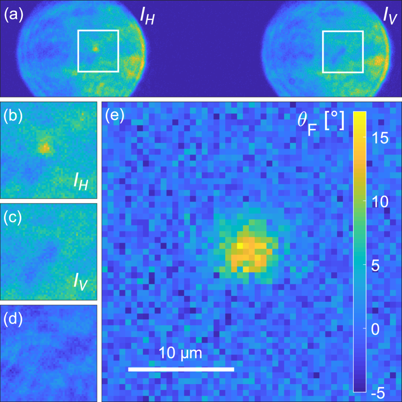
Figure 2: Dual Port Faraday Imaging. Panel (a) displays the raw polarisation image obtained on the camera. The two white frames enclose the area shown in panels (b) and (c) which contain the raw polarisation fields $I_{\rm H}$ and $I_{\rm V}$ respectively. The colourscale in panels (a)-(c) represent the light intensity. Panel (d) is an averaged Faraday image without atoms and (e) contains the final Faraday image. The colourscale of panel (d) is the same as that of (e).

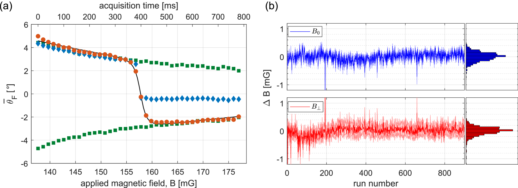
Figure 3: Vector magnetometry. (a) A typical trace of a single magnetometer sequence as a function of the applied magnetic field is shown in red ($\bullet$). The data are fit using eq. (2), and the result is shown as the black solid line. The blue trace ($\blacklozenge$) occurs when the background fields are compensated below the threshold for Majorana losses. The green ($\blacksquare$) curves show the intrinsic signal loss during probing; they are produced by keeping the bias field at a fixed value. The top axis shows the acquisition time of the magnetic field sweep. The absolute calibration of the applied field was obtained using the Larmor magnetometer presented in Sec. IV. (b) Long term magnetic field drift. The magnetometer was operated continuously for about 900 experimental runs and the magnetic field values extracted for each run, $B_{0}$ (blue) and $B_{\perp}$ (red). The shaded areas are $1\sigma$ errors of the fits. The histograms are rendered from the fit results.

III Vectorial magnetometry

In a first set of experiments, a vectorial magnetometer was implemented by taking Faraday images of an atomic cloud while the magnetic field is changed in amplitude and direction. As long as the field sweep is slow compared to the instantaneous Larmor frequency, the orientation of the collective spin of the atomic cloud follows the magnetic field direction. Hence, a magnetic field parallel to the Faraday beam will lead to $\braket{f_{z}}>0$ and positive $\theta_{F}$. Likewise an antiparallel field component will result in $\braket{f_{z}}<0$ and negative $\theta_{F}$. When the parallel field component vanishes, $\theta_{F}$ is zero.

The magnetometer sequence is implemented as follows: After evaporative cooling of the atomic cloud in the CDT, the collective atomic spin is prepared either parallel or antiparallel to the probing direction by raising an offset field within $200$ ms in the respective direction. Subsequently, a train of $40$ Faraday pulses is triggered. Each pulse is $2~{}\mu$s in duration and has an intensity of $150$ pW$/\mu$m². The light is $1.13$ GHz blue detuned with respect to the $F=2\rightarrow F^{\prime}=3$ transition of the ⁸⁷Rb D2 line. The images are acquired at a rate of $f_{\rm aq}=50$ Hz, such that the total measurement time is $780$ ms. This rate is chosen to minimise the shot-to-shot jitter due to the $50$ Hz line frequency. Simultaneously the magnetic field component along the Faraday beam is swept through $\Delta B=40$ mG at a sweep speed of $50~{}$mG/s. Since the field sweep must be slow compared to the instantaneous Larmor frequency, the maximal speed is set by the residual transverse magnetic field, $B_{\perp}$. By averaging over a given region of interest (ROI) in the Faraday images, we can obtain a signal evolving as a function of acquisition time, reproducing the dynamics of the magnetic field.

A typical trace is shown in red in Fig. 3 (a), where the mean rotation angle, $\bar{\theta}_{F}$, in a ROI of $20\times 40~{}\mu$m² was used. In our case, the external field is swept at a constant rate leading to a linear relation between the acquisition time (bottom axis) and magnitude of the applied field (top axis). Initially, the signal falls off slowly due to losses caused by the probe light itself. When the field strength reaches a critical value, the transverse components begin to dominate the total magnetic field vector and the signal drops significantly since the collective atomic spin turns with the field. The signal changes sign and the zero crossing corresponds to the instance where the field component along the probe direction is zero. At this point the background magnetic field and the applied field, $B_{0}$, are equal and opposite, cancelling each other. The width of the zero crossing is related to the magnitude of $B_{\perp}$.

To extract values for the magnetic field components we fit the measured $\bar{\theta}_{F}$ as a function of the applied field $B$ with the expression Gajdacz et al. (2013)

$$\bar{\theta}_{F}(B)=-Ae^{-k{B}}\frac{(B-B_{0})}{\sqrt{(B-B_{0})^{2}+B_{\perp}^{2}}}.$$ (2)

This is based on the assumption that the rotation angle adiabatically follows the magnetic field vector. The loss of signal due to the probe itself is modelled by an exponential decay with decay constant $k$ assuming a constant sweep rate of $B$ . The remaining expression corresponds to the projection of the total magnetic field vector, $\mathbf{B}=(B-B_{0},B_{\perp})$, onto the probe direction. The parallel and perpendicular magnetic field values $B_{0}$ and $B_{\perp}$ as well as the amplitude $A$ are free fit parameters. Based on this procedure it is clear that the accuracy of the measured field values relies on the calibration of the magnetic coils used for the sweep of the applied field.

For the trace shown in Fig. 3, the fit yields values of $B_{0}=157.87$ mG and $B_{\perp}=1.3$ mG, with single-shot $1\sigma$ precision of $\delta B_{0}=0.05$ mG and $\delta B_{\perp}=0.1$ mG. An implementation of this particular kind of a cold atom magnetometer, was demonstrated in Gajdacz et al. (2013), inspired by older spectroscopic scanning-field techniques Dupont-Roc et al. (1969). However the measurement in Gajdacz et al. (2013) was not sensitive to the polarisation direction of the spin ensemble. Our realisation represents an improvement of the single-shot precision by two orders of magnitude.

Even though the Faraday probe is more than a GHz off-resonant, it induces signal loss via heating and transfer to different magnetic states. To characterise this loss we have performed a Faraday measurement while keeping the value of the magnetic field fixed. These traces are shown in green in Fig. 3 (a) and correspond to the decay caused by the imaging procedure itself. The different signs of the traces represent atomic clouds initially prepared with collective spins pointing in parallel (positive) and antiparallel (negative) directions, with respect to the probe beam.

When the transverse background fields are well compensated we see a dramatically different behaviour (Fig. 3 (a), blue trace). The population of the initial spin state is lost due to Majorana spin flips, since the total field becomes close to zero. A loss in the spin signal is expected when the relative rate of change in the magnetic field $|\frac{1}{B}\frac{dB}{dt}|$ becomes higher than the Larmor frequency. Hence, for the sweep speeds presented here, the fields must be compensated to within $0.2$ mG. This corresponds to the level of the passive compensation of the background fields in our experiment.

The vectorial magnetometer was used to measure the background field drifts over a period of $8$ hours, as shown in Fig. 3 (b). We compare the magnetic field trace to its mean value using $\Delta B=B(t)-\bar{B}$. The $1\sigma$ deviation of the histograms of both the parallel and transversal field components amounts to about $0.2$ mG, which is a typical performance in an unshielded environment. Most notably, the single-shot precision is better than typical shot-to-shot fluctuations, which renders the method eligible for improving measurements of atomic properties that depend crucially on the background magnetic field. In such cases one must measure the background field during the experiment and either actively compensate for its effect Smith et al. (2011) or post select from the data according to the value measured Bason et al. (2018); Krinner et al. (2018).

In the context of our experiment, this method mainly serves as a probe upon which subsequent measurements or dynamics can be conditioned. For completeness, we also quote the sensitivities, corresponding to the single-shot magnetic field precision normalized to the total running time of one measurement, as is customary for optical magnetometers . At the full experimental cycle of $30$ s, this yields sensitivities of $\delta B_{0}\sqrt{T}=27$ nT Hz${}^{-\frac{1}{2}}$ and $\delta B_{\perp}\sqrt{T}=55$ nT Hz${}^{-\frac{1}{2}}$

Thus, the fields $B_{0}$ and $B_{\perp}$ are obtained with a precision that is much lower than shot-to-shot fluctuations in a single realisation of the experiment, despite the simplicity of the measurement scheme. However, its accuracy relies on the quality of the external field calibration.

IV Larmor magnetometry

In a second set of experiments, a magnetometer based on Larmor precession was implemented. Generally, a spin polarised atomic ensemble precesses in a magnetic field if the polarisation is tilted with respect to the field. Since the Larmor frequency is $\omega_{L}=\gamma B$ for small fields, where $\gamma$ is the gyromagnetic ratio, the magnetic field strength $B$ can be measured accurately by measuring $\omega_{L}$. In our case using the $\ket{F=2,m_{F}=2}$ state of ⁸⁷Rb, the Larmor frequency is given by $\omega_{L}/B=2\pi\times 1.4~{}$MHz/G Steck (2010).

Larmor magnetometry has commonly been applied using cold and ultracold atoms. Moreover fast phase contrast imaging has been applied to measure the phase acquired by a precessing BEC in a synthetic magnetic field Vengalattore et al. (2007), yielding single-shot precision of $9$ nG. High-resolution gradient magnetometry was performed at a precision of about $100$ nG$/\mu$m Higbie et al. (2005); Koschorreck et al. (2011); Muessel et al. (2014a). The method has also been used to measure field curvatures of a quadrupolar field in multiple experimental realisations on the mm scale Fatemi and Bashkansky (2010). Here we apply an established method of magnetometry and put it in the context of spatially-resolved probing that could enable the reduction of detrimental effects induced by environmental fluctuations on magnetic field sensitive atomic dynamics.

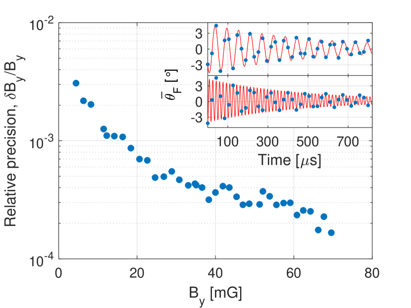
Figure 4: Larmor magnetometry. The Larmor magnetometer was tested for a range of magnetic field strengths. The relative precision of the measurement increases with increasing field. The inset shows experimental data for the Larmor magnetometer as blue dots, and fits as the red solid lines. In the top panel the measured field was 12.253(13) mG and in the bottom panel 41.894(17) mG. Note that the field of the latter measurement corresponds to Larmor frequencies above $f_{\rm aq}$ which was taken into account in the fit procedure.

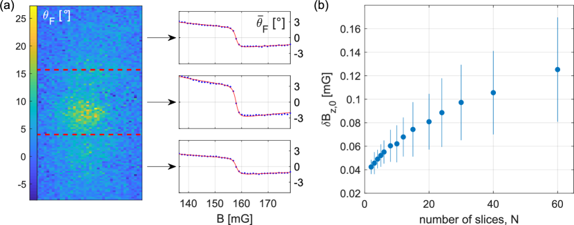
Figure 5: Spatially-resolved detection. (a) Individual images of a single run of the vectorial magnetometer are analyzed in multiple slices (here in $N=3$ slices) along the long extension of the cloud. The $3$ graphs display the mean Faraday angle and the fitted magnetometer trace, and the image is the first frame in the series. (b) The procedure was applied for a varying number of slices $N$ and the average precision as a function of the number of slices $N$ is shown. The error bar represents $1\sigma$ of the $N$ fitted precisions.

The experimental sequence starts by preparing a cold spin polarised thermal cloud of $\ket{2,2}$ atoms in the CDT. Thereafter, a single additional tweezer is ramped to a potential depth of about $2~{}\mu$K, holding about $1000$ atoms. By doing so, we locally enhance the optical density of the cloud, and thereby allow for an improvement of the Faraday signal. Since these experiments measure an applied magnetic field component along the vertical direction ($y$-axis), $B_{\perp}=\sqrt{B_{x}^{2}+B_{y}^{2}}$ is initially compensated to below $0.2~{}$mG and the longitudinal field is set to $B_{0}=5$ mG along the probing direction in order to maintain the magnetisation of the cloud. To initiate Larmor precession, a magnetic field is abruptly turned on in the vertical direction. The initial ramp speed of $5~{}$mG/$\mu$s is large enough such that the spin polarisation does not follow, and the collective spin state starts to precess around the $y$-axis. Thereafter the magnetic field along the $z$-direction is nulled. Precisely $20$ ms later – one cycle of the $50$ Hz power line – the field along the $y$-axis is turned on and a Faraday pulse train is started. By operating the EMCCD in fast kinetic mode and selecting a ROI of only $25$ pixels height around the Faraday signal of the atoms, we reach an acquisition frequency of $f_{\rm aq}=44.31(2)$ kHz, resulting in a total probing time of $T_{\rm aq}=925~{}\mu$s. The acquisition procedure is similar to the one presented in Higbie et al. (2005). Typical measurement results are shown in the two insets of Fig. 4, where the mean rotation angle in a ROI of $5\times 5~{}\mu m^{2}$ ($10\times 10$ camera pixels) was used to extract the measured quantities. By fitting an exponentially damped sinusoidal oscillation to the trace we extract the Larmor frequency. Thus, we can determine the magnetic field to a $1\sigma$ precision of $\delta B_{y}=15\ \mu$G in a single realisation of the experiment. Given the full experimental cycle time of $T=30~{}$s this corresponds to a sensitivity of $\delta B_{y}\sqrt{T}=8$ nT Hz${}^{-\frac{1}{2}}$.

To test the dynamic range of the magnetometer we performed the experiment for a range of magnetic field strengths from $3$ mG to $70$ mG. The absolute precision is roughly constant over the range of measured field strengths and hence the relative precision increases, as shown in Fig. 4.

This method provides an accurate way of measuring the magnetic field at the atomic cloud position. It can be used to measure higher magnetic fields than with the vectorial magnetometer covered above in Sec. III. As a potential, improvement the Larmor precession could be initiated via optical pumping instead of a sudden field change. In that way the initial phase of the oscillation can be fixed. Moreover, this method would also allow for a spatially-selective way of initiating the precession. This would be necessary for a magnetometer sequence which uses spatially-selective probing. In the following section we extend the magnetometer sequences and demonstrate the capabilities to perform such measurements.

V Spatial probing and detection schemes

Our experimental setup offers possibilities of both spatially-resolved detection and spatially-selective probing. The spatial resolution of the detection is due to the fact that the Faraday signal is recorded on a camera, where conventionally it is only measured with a photo detector. The spatial selectivity in probing is enabled by shaping of the Faraday probe light with a DMD.

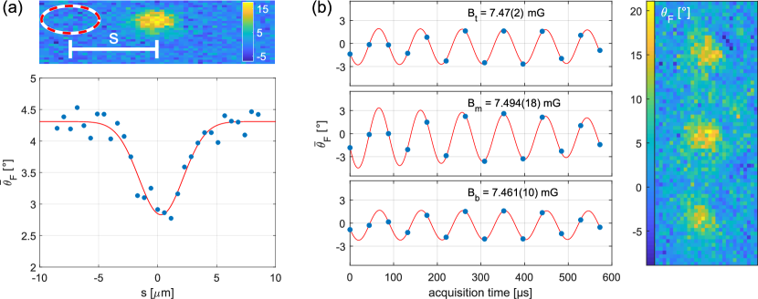
Figure 6: Spatially-selective probing. (a) Locality of the probe light. The atoms are only affected by the DMD shaped probe beam if the probe light overlaps the atomic cloud. (b) Larmor magnetometry in an array. The Larmor magnetometer was applied to atoms in a $3\times 1$ array of tweezers, shown in the right panel. The obtained magnetic field values are printed in Larmor precession traces to the left.

Generally, the best signal-to-noise-ratio is obtained when the total Faraday signal from the whole cloud is recorded. This can be realised by summing the measured Faraday rotation pixel by pixel, which is essentially the same as using a photo detector. Such a situation will however inhibit spatially-resolved detection of the magnetic fields in different microtraps, as the spatial information in the image is not used.

To investigate the single-shot precision between the limiting cases of using the full spatial resolution or summing all the signal, we use the measurements taken with the vectorial magnetometer, shown in Fig. 3 (a). The dataset consists of $40$ Faraday images with a size of $20\times 60~{}\mu$m² ($40\times 120$ camera pixels). In our analysis, each image is split into $N$ slices along the longer side of the cloud and $\bar{\theta}_{F}$ is obtained for each slice, yielding $N$ magnetometry traces, as shown in Fig. 5 (a). Equation 2 is fitted to each trace, providing $N$ values for the fit precision $\delta B_{0}$. Fig. 5 (b) shows the mean and the standard deviation of the precision as a function of the chosen number of slices. As the number of slices $N$ grows, the determination of the magnetic field value becomes less precise, according to expectations.

This result clearly demonstrates the advantages of spatially-resolved detection. The chosen value of $N$ corresponds to the ability to measure the shape of the magnetic field to the $N$-th power, which is useful when mapping complex magnetic field structures such as at the surface of microscopic electronic chips Wildermuth et al. (2005). In particular, we can reach a gradient precision of $3~{}\mu$G$/\mu$m with the vectorial magnetometer.

The spatial control of the Faraday imaging light enables spatially-selective probing in our experimental implementation. In particular a number of atomic samples can be probed in an array of traps, without disturbing the remaining samples. It is therefore important to determine the detrimental effect of a given local Faraday measurement on an atomic cloud in a microtrap as a function of the distance between them. This is realised as follows: first, a single microtrap is loaded as described above. Then the DMD is used to produce a Faraday probe beam with a waist of about $3.8~{}\mu$m, at a variable position relative to the atomic cloud. In each experimental realisation, two sequential Faraday images are taken in which the position of the probe beam in the first image is variable, whereas the probe beam always hits the atomic cloud in the second image. The measurement principle is illustrated in the top panel of Fig. 6 (a), where the red circle marks the position of the probe beam in the first shot, with respect to the cloud situated at a distance $s$. The separation $s$ is scanned and the mean rotation angle as measured from the second Faraday image is shown. The effect of the first probe is clear from the reduced Faraday signal in the centre of the graph. The width, extracted from a Gaussian fit is $3.8(3)~{}\mu$m, in good agreement with the probe beam size. This illustrates that the effect of the probe beam is minimal when it does not hit the cloud. The extinction ratio of the DMD is thus good enough to completely eliminate the need of screening of any residual light which might originate from the Faraday light source.

Finally the potential of a spatially-selective probing scheme is further illustrated by appling the Larmor magnetometer to a triple tweezer system as shown in Fig. 6 (b). The atomic clouds are separated by $13~{}\mu$m. In this realisation $14$ Faraday images were taken in $570~{}\mu$s and the traces fitted with a damped sinusoid. The result allows us to put an upper bound on a magnetic field gradient at $\frac{dB}{dy}~{}=1.5~{}\mu$G$/\mu$m. This is only about one order of magnitude less precise than the best cold atoms gradiometers to date Koschorreck et al. (2011); Muessel et al. (2014b), but in contrast to those realisations ours can be applied in-sequence with other measurements on the same atomic cloud.

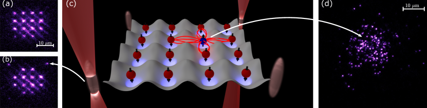
Figure 7: Proposal for enhanced quantum simulations using the spatially-selective probing scheme. (a) Fluorescence image of a 4 by 4 tweezer array of atomic clouds. The trapping potential is generated by a DMD using 940 nm laser light and projected through our newly established quantum gas microscope. (b) Subsequently, using the dynamic capabilities of the DMD, the four corner traps are moved outwards. (c) The corner traps now can serve for instance as selective magnetic field probing regions without affecting magnetic sensitive quantum spin dynamics taking place in the centre region. (d) As an example of the interaction region, we show a fluorescence image of single atoms sparsely populating an optical lattice demonstrating the functionality of our quantum gas microscope.

VI Outlook

We have presented two types of magnetometers that both rely on the Faraday imaging technique. One is vectorial in nature where we reach single-shot precisions of $\delta B_{0}=50~{}\mu$G and $\delta B_{\perp}=100~{}\mu$G of the magnetic fields parallel and transverse to the direction of the Faraday probe. The achieved precision is two orders of magnitude better than a previous realisation Gajdacz et al. (2013). The second magnetometer is based on Larmor precession, making it both accurate and precise, reaching a single-shot precision of $\delta B_{y}=15\ \mu$G.

The dispersive nature of the measurement technique applied allows it to be conducted in sequence with other experiments on cold atoms. This concept was recently demonstrated in Bason et al. (2018) and in the context of magnetometry in Krinner et al. (2018). Our setup is equipped to create arrays of tweezers that can be individually probed without disturbing the atoms in neighbouring traps. In this way one can perform gradient or tensorial magnetometry and with improvements of the apparatus similar to Chisholm et al. (2018), the trapping potential could also be made three-dimensional, enabling full $3$D magnetic field mapping. The spatially-selective aspect of the technique also allows one to perform magnetic field sensitive measurements in a portion of the system while monitoring the magnetic field in another part. In our case an atomic system could be split into arbitrarily many spatially distributed sensor regions where the magnetic field is sensed, and an interaction region where magnetic field sensitive dynamics take place.

The experimental setup described in this paper has recently been extended to include a quantum gas microscope. It features a $0.70$ NA microscope objective capable of imaging atoms pinned in a deep 3D cubic optical lattice at the resolution of a single lattice site. Figure 7 (d) is an example of such an image. Each bright spot corresponds to the fluorescent photons from an individual atom trapped in the lattice. Additionally, atoms can be trapped in flexible DMD generated conservative trapping potentials produced with $940$ nm light allowing for dynamic control of the energy landscape. The potential of this feature is shown in Fig. 7 (a) and (b). In this experiment 16 atomic clouds were trapped in a 4 by 4 array of optical tweezers, each with a waist of about $1.0~{}\mu$m (a). The corners of the array are then moved diagonally outwards by $5~{}\mu$m (b). As illustrated in Fig. 7 (c), the four corners can now form four sensing regions for magnetic field measurements. They are disconnected from the central region which remains unaffected and could be used for the quantum simulation of complex many-body physics of atoms in optical lattices.

In contrast to previous multimode probing schemes that were performed on a bulk atomic cloud Pu et al. (2017), limitations on quantum memory lifetimes due to atomic motion in the bulk cloud can be circumvented by such a combination of trapping and manipulation of individual atoms in tweezer arrays together with spatially-selective dispersive probing. In addition, all the individual probing beams are collected on a camera with sufficient resolution to detect each cloud individually. This opens the possibility for simultaneous probing of several clouds, which is not possible when all signals are combined on a single detector.