Overcoming resolution limits with quantum sensing

T. Gefen Racah Institute of Physics, The Hebrew University of Jerusalem, Jerusalem 91904, Givat Ram, Israel    A. Rotem Racah Institute of Physics, The Hebrew University of Jerusalem, Jerusalem 91904, Givat Ram, Israel    A. Retzker Racah Institute of Physics, The Hebrew University of Jerusalem, Jerusalem 91904, Givat Ram, Israel
(March 9, 2024)
Abstract

The field of quantum sensing explores the use of quantum phenomena to measure a broad range of physical quantities, of both static and time-dependent types. An important figure of merit for time dependent signals is the spectral resolution, i.e. the ability to resolve two different frequencies. Here we study this problem, and develop new superresolution methods that rely on quantum features. We first formulate a general criterion for superresolution in quantum problems. Inspired by this, we show that quantum detectors can resolve two frequencies from incoherent segments of the signal, irrespective of their separation, in contrast to what is known about classical detection schemes. The main idea behind these methods is to overcome the vanishing distinguishability in resolution problems by nullifying the projection noise.

Introduction

Quantum metrology and quantum sensing Giovannetti et al. (2011); Degen et al. (2017) study parameter estimation limits in various physical systems by employing the fundamental laws of quantum physics. In particular this field seeks to optimize precision by utilizing quantum effects that have no classical analogs (such as entanglement and squeezing Bollinger et al. (1996); Itano et al. (1993)).

A unique feature of quantum sensing is the ability to apply coherent control to the probe and vary the measurement basis. In particular this provides the ability to nullify the measurement projection noise. However, the contribution of this phenomenon to estimation problems has received scant attention.

In this paper we highlight this feature and show that it is a critical resource primarily for resolution problems, that can improve precision by orders of magnitude. Resolution problems are ubiquitous and highly important in science Rayleigh (1879); Hannan and Quinn (1989); Hell and Wichmann (1994); Bettens et al. (1999); Van Aert et al. (2002); Tsang et al. (2016); Nair and Tsang (2016a); Lupo and Pirandola (2016); Barabell et al. (1998); Glentis et al. (2014), and roughly speaking are characterized by vanishing distinguishability; i.e, the sensitivity to the seperation between two close objects or frequencies vanishes as these get close enough. This effect usually results in divergent uncertainty, leading to a resolution limit. We show that it is possible to overcome the vanishing distinguishability by making the projection noise vanish as well, through a suitable control. These two effects can cancel each other out, leading to a finite uncertainty. We show that this is a general method to overcome resolution limits in quantum sensing.

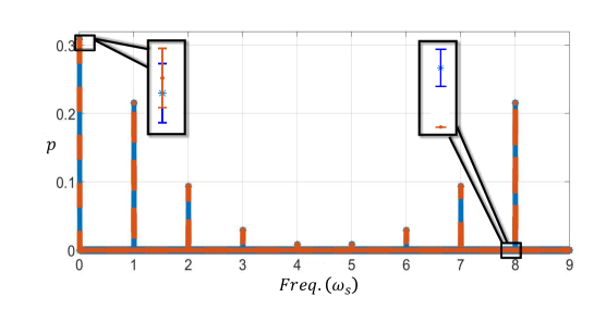
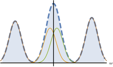
Specifically, this method can be highly useful for analyzing complex spectrums with quantum sensors (such as quantum NMR problems Staudacher et al. (2013); Aslam et al. (2017); Pham et al. (2016); Kong et al. (2015)). An example for such a spectrum is illustrated in fig. 1 . While the two extreme frequencies can easily be estimated, the two central frequencies must be analyzed with a more sophisticated method, which eventually yields higher uncertainty. Here, we show that by using a quantum control, the spectrum can be shifted such that the projection noise vanishes. The vanishing projection noise implies a finite uncertainty irrespective of the frequency separation. In other words, the uncertainty does not diverge when the two frequencies merge. Furthermore, this method is extremely simple, unlike numerically demanding classical superresolution methods.
Refer to caption
Figure 1: A spectrum analysis problem. While it is relatively easy to estimate the two side frequencies, the estimation of the two close frequencies is challenging and becomes infinitely difficult when the frequencies merge.

Results

.1 Conditions for superresolution

We first briefly review the pillars of quantum parameter estimation problems. A typical problem involves a quantum state ρ(θ),𝜌𝜃\rho\left(\theta\right), such that θ𝜃\theta is to be estimated. The uncertainty in estimating θ𝜃\theta is tightly lower bounded by 1Iθ1subscript𝐼𝜃\frac{1}{\sqrt{I_{\theta}}} , where Iθsubscript𝐼𝜃I_{\theta} is the Fisher information (FI) about θ𝜃\theta Cramér (2016). For a given choice of measurement of ρ(θ),𝜌𝜃\rho\left(\theta\right), Iθsubscript𝐼𝜃I_{\theta} is determined according to the probabilities (pj)subscript𝑝𝑗\left(p_{j}\right) in the following way: Iθ=j(dpjdθ)2pj.subscript𝐼𝜃subscript𝑗superscript𝑑subscript𝑝𝑗𝑑𝜃2subscript𝑝𝑗I_{\theta}=\sum_{j}\frac{\left(\frac{dp_{j}}{d\theta}\right)^{2}}{p_{j}}. The FI can be optimized over all possible measurements, leading to the quantum Fisher information (QFI) Wootters (1981); Braunstein and Caves (1994). Given a spectral decomposition ρ=jpj|ψjψj|𝜌subscript𝑗subscript𝑝𝑗ketsubscript𝜓𝑗brasubscript𝜓𝑗\rho=\sum_{j}p_{j}|\psi_{j}\rangle\langle\psi_{j}| the QFI about θ𝜃\theta reads: =pi+pj02pj+pi|(dρdθ)i,j|2.subscript𝑝𝑖subscript𝑝𝑗02subscript𝑝𝑗subscript𝑝𝑖superscriptsubscript𝑑𝜌𝑑𝜃𝑖𝑗2\mathcal{F}=\underset{p_{i}+p_{j}\neq 0}{\sum}\frac{2}{p_{j}+p_{i}}\bigg{|}\left(\frac{d\rho}{d\theta}\right)_{i,j}\bigg{|}^{2}.

For a multivariable estimation of {θk}k,subscriptsubscript𝜃𝑘𝑘\left\{\theta_{k}\right\}_{k}, the error is quantified by the covariance matrix of the estimators. This covariance matrix is lower bounded by 1,superscript1\mathcal{F}^{-1}, the inverse of the QFI matrix, where the QFI matrix is defined as k,l=2i,j(ρθk)i,j(ρθl)j,i(pi+pj).subscript𝑘𝑙2𝑖𝑗subscript𝜌subscript𝜃𝑘𝑖𝑗subscript𝜌subscript𝜃𝑙𝑗𝑖subscript𝑝𝑖subscript𝑝𝑗\mathcal{F}_{k,l}=2\underset{i,j}{\sum}\frac{\left(\frac{\partial\rho}{\partial\theta_{k}}\right)_{i,j}\left(\frac{\partial\rho}{\partial\theta_{l}}\right)_{j,i}}{\left(p_{i}+p_{j}\right)}.

We are now poised to formulate spectral resolution problems, which are the focus of this paper. In these problems we are given a signal (Hamiltonian) that oscillates with time. It consists of at most two frequencies, yet the exact number of frequencies (and their values) is unknown and need to be determined. To this end, a quantum probe interacts with the signal so that information about it becomes encoded on the probe and can be extracted by measurements. Once this information is extracted this problem boils down to a parameter estimation problem: the common strategy in these problems Hannan and Quinn (1989); Barabell et al. (1998); Roy and Kailath (1989); Rotem et al. (2019) is to assume that there are two frequencies and estimate them. If the estimation shows a significant overlap between the frequencies (significant with respect to the estimation error), it is concluded that the frequencies are not resolvable. However if the overlap is negligible, one can deduce that the signal consists of two frequencies (since the error probability is negligible). This implies that the figure of merit is Δω1,Δsubscript𝜔1\Delta\omega_{1}, Δω2.Δsubscript𝜔2\Delta\omega_{2}. The challenging regime is when ω1ω2.subscript𝜔1subscript𝜔2\omega_{1}\rightarrow\omega_{2}. Resolution becomes an issue when Δω1,Δω2Δsubscript𝜔1Δsubscript𝜔2\Delta\omega_{1},\>\Delta\omega_{2}\rightarrow\infty as ω1ω2.subscript𝜔1subscript𝜔2\omega_{1}\rightarrow\omega_{2}. A different, and somewhat more convenient, formulation uses ωr=ω1ω22,subscript𝜔rsubscript𝜔1subscript𝜔22\omega_{\mathrm{r}}=\frac{\omega_{1}-\omega_{2}}{2}, ωs=ω1+ω22,subscript𝜔ssubscript𝜔1subscript𝜔22\omega_{\mathrm{s}}=\frac{\omega_{1}+\omega_{2}}{2}, so that the resolution condition is Δωrωrmuch-less-thanΔsubscript𝜔rsubscript𝜔r\Delta\omega_{\mathrm{r}}\ll\omega_{\mathrm{r}} and the figure of merit is thus Δωr.Δsubscript𝜔r\Delta\omega_{\mathrm{r}}. The key issue is thus the behavior of ΔωrΔsubscript𝜔r\Delta\omega_{\mathrm{r}} as ωr0,subscript𝜔r0\omega_{\mathrm{r}}\rightarrow 0, if ΔωrΔsubscript𝜔r\Delta\omega_{\mathrm{r}}\rightarrow\infty then a fundamental resolution limit exists which is the case in relevant classical examples Hannan and Quinn (1989); Barabell et al. (1998); Roy and Kailath (1989).

This limitation appears in various resolution problems (not only spectral resolution) and stems from a property of vanishing distinguishability. Let us define what vanishing distinguishability means. Given the quantum state of a probe (density matrix ρ𝜌\rho), that depends on a set of parameters {θi}i,subscriptsubscript𝜃𝑖𝑖\left\{\theta_{i}\right\}_{i}, the state suffers from a vanishing distinguishability if the set (ρθi)isubscript𝜌subscript𝜃𝑖𝑖\left(\frac{\partial\rho}{\partial\theta_{i}}\right)_{i} is linear dependent. An equivalent way to define it: there exists a parameter g,𝑔g, that is a linear combination of {θi}i,subscriptsubscript𝜃𝑖𝑖\left\{\theta_{i}\right\}_{i}, such that ρg=0.𝜌𝑔0\frac{\partial\rho}{\partial g}=0. Indeed, in many resolution problems as the separation parameter ωrsubscript𝜔r\omega_{\mathrm{r}} (the difference between the frequencies or , in imaging, the sources) goes to 0,00, there exists a parameter g𝑔g such that ρg=0.𝜌𝑔0\frac{\partial\rho}{\partial g}=0. In this paper we focus on the simplest (yet very common) case that only ρωr=0𝜌subscript𝜔r0\frac{\partial\rho}{\partial\omega_{\mathrm{r}}}=0 as ωr=0.subscript𝜔r0\omega_{\mathrm{r}}=0. In this case ΔωrΔsubscript𝜔r\Delta\omega_{\mathrm{r}}\rightarrow\infty if and only if the FI about ωrsubscript𝜔r\omega_{\mathrm{r}} (denoted as Irsubscript𝐼rI_{\mathrm{r}}) vanishes, which implies that Irsubscript𝐼rI_{\mathrm{r}} is our figure of merit.

As an example, consider a signal that acts on a qubit and is given by the following Hamiltonian:

H=[A1cos(ω1t)+B1sin(ω1t)+A2cos(ω2t)+B2sin(ω2t)]σz.𝐻delimited-[]subscript𝐴1subscript𝜔1𝑡subscript𝐵1subscript𝜔1𝑡subscript𝐴2subscript𝜔2𝑡subscript𝐵2subscript𝜔2𝑡subscript𝜎𝑧H=\left[A_{1}\cos\left(\omega_{1}t\right)+B_{1}\sin\left(\omega_{1}t\right)+A_{2}\cos\left(\omega_{2}t\right)+B_{2}\sin\left(\omega_{2}t\right)\right]\sigma_{z}. (1)

It is simple to see that this limitation appears whenever the Hamiltonian posses a symmetry for exchange of ω1ω2subscript𝜔1subscript𝜔2\omega_{1}\leftrightarrow\omega_{2} (i.e. identical amplitudes). This symmetry implies a symmetry of ωrωr,subscript𝜔rsubscript𝜔r\omega_{\mathrm{r}}\leftrightarrow-\omega_{\mathrm{r}}, from which it follows that the state obtained after evolution time t𝑡t has the same symmetry,|ψt(ωr)=|ψt(ωr)ketsubscript𝜓𝑡subscript𝜔rketsubscript𝜓𝑡subscript𝜔r|\psi_{t}\left(\omega_{\mathrm{r}}\right)\rangle=|\psi_{t}\left(-\omega_{\mathrm{r}}\right)\rangle, and thus |ψtωr=0ketsubscript𝜓𝑡subscript𝜔r0\frac{\partial|\psi_{t}\rangle}{\partial\omega_{\mathrm{r}}}=0 for ωr=0.subscript𝜔r0\omega_{\mathrm{r}}=0. Given the expression of the quantum Fisher information Braunstein and Caves (1994), we obtain:

Ir4[ψωr|ψωr|ψωr|ψ|2]0,subscript𝐼r4delimited-[]inner-product𝜓subscript𝜔r𝜓subscript𝜔rsuperscriptinner-product𝜓subscript𝜔r𝜓20I_{\rm{r}}\leq 4\left[\left\langle\frac{\partial\psi}{\partial\omega_{\mathrm{r}}}\bigg{|}\frac{\partial\psi}{\partial\omega_{\mathrm{r}}}\right\rangle-\left|\left\langle\frac{\partial\psi}{\partial\omega_{\mathrm{r}}}\bigg{|}\psi\right\rangle\right|^{2}\right]\rightarrow 0, (2)

hence resolution is limited. Note that applying further control on the probe cannot eliminate this symmetry, and thus cannot remove this resolution limit.

It can be shown that this limitation appears for any quadratures: there exists a parameter g𝑔g such that Hg=0𝐻𝑔0\frac{\partial H}{\partial g}=0 for every t,𝑡t, which implies |ψtg=0ketsubscript𝜓𝑡𝑔0\frac{\partial|\psi_{t}\rangle}{\partial g}=0 for every measurement (more details in supplementary note 4).

So vanishing distinguishability is quite a common property and appears in different resolution problems, but does it always impose a limitation?

Eq. 2 shows that whenever the quantum state of the probe (ρ𝜌\rho) is pure, resolution is limited, however for some mixed states this property does not limit the resolution, these are the states that give rise to superresolution: dρdωr=0𝑑𝜌𝑑subscript𝜔r0\frac{d\rho}{d\omega_{\mathrm{r}}}=0 yet Ir(ωr0)>0.subscript𝐼rsubscript𝜔r00I_{{\rm r}}\left(\omega_{{\rm r}}\rightarrow 0\right)>0. A special case of this phenomenon was found and analyzed recently in the context of optical imaging Nair and Tsang (2016a); Tsang et al. (2016); Lupo and Pirandola (2016); Chrostowski et al. (2017)(see supplementary note 3). Can such states be obtained in quantum spectroscopy and various other problems? In order to understand this, it would be highly desirable to characterize these states and set a sharp condition for superresolution.

Let us show that these states can be simply characterized:

Claim: Given ρ(ωr)𝜌subscript𝜔r\rho\left(\omega_{\mathrm{r}}\right) such that dρdωr=0𝑑𝜌𝑑subscript𝜔r0\frac{d\rho}{d\omega_{\mathrm{r}}}=0 (as ωr0subscript𝜔r0\omega_{\mathrm{r}}\rightarrow 0), then Ir(ωr0)>0subscript𝐼rsubscript𝜔r00I_{{\rm r}}\left(\omega_{{\rm r}}\rightarrow 0\right)>0 if and only if at least one of the eigenvalues of ρ𝜌\rho goes as ωrk,superscriptsubscript𝜔r𝑘\omega_{\mathrm{r}}^{k}, where 1<k21𝑘21<k\leq 2 or equivalently dρdωr0𝑑𝜌𝑑subscript𝜔r0\frac{d\sqrt{\rho}}{d\omega_{\mathrm{r}}}\neq 0. The optimal measurement basis converges to an eigenbasis of ρ𝜌\rho as ωr0subscript𝜔r0\omega_{\mathrm{r}}\rightarrow 0.

We briefly illustrate a proof: Given a spectral decomposition ρ=𝑗pj|jj|,𝜌𝑗subscript𝑝𝑗ket𝑗bra𝑗\rho=\underset{j}{\sum}p_{j}|j\rangle\langle j|, then:

dρdωr=𝑗dpjdωr|jj|+ij,k(pjpk)hk,j|kj|,𝑑𝜌𝑑subscript𝜔r𝑗𝑑subscript𝑝𝑗𝑑subscript𝜔rket𝑗quantum-operator-product𝑗𝑖𝑗𝑘subscript𝑝𝑗subscript𝑝𝑘subscript𝑘𝑗𝑘bra𝑗\frac{d\rho}{d\omega_{\rm{r}}}=\underset{j}{\sum}\frac{dp_{j}}{d\omega_{\rm{r}}}|j\rangle\langle j|+i\underset{j,k}{\sum}\left(p_{j}-p_{k}\right)h_{k,j}|k\rangle\langle j|, (3)

where hh is a Hermitian operator and hk,jsubscript𝑘𝑗h_{k,j} denote its matrix elements in the eigenbasis of ρ𝜌\rho. Since dρdωr0𝑑𝜌𝑑subscript𝜔r0\frac{d\rho}{d\omega_{\mathrm{r}}}\rightarrow 0, then for every j,k𝑗𝑘j,k: dpjdωr0,(pjpk)hk,j0.formulae-sequence𝑑subscript𝑝𝑗𝑑subscript𝜔r0subscript𝑝𝑗subscript𝑝𝑘subscript𝑘𝑗0\frac{dp_{j}}{d\omega_{\mathrm{r}}}\rightarrow 0,\;\left(p_{j}-p_{k}\right)h_{k,j}\rightarrow 0. With this notation, the QFI (\mathcal{F}) reads (see Braunstein and Caves (1994)):

=𝑗(dpjdωr)2pj+2j,k(pjpk)2pj+pk|hkj|2.𝑗superscript𝑑subscript𝑝𝑗𝑑subscript𝜔r2subscript𝑝𝑗2𝑗𝑘superscriptsubscript𝑝𝑗subscript𝑝𝑘2subscript𝑝𝑗subscript𝑝𝑘superscriptsubscript𝑘𝑗2\mathcal{F}=\underset{j}{\sum}\frac{\left(\frac{dp_{j}}{d\omega_{\mathrm{r}}}\right)^{2}}{p_{j}}+2\underset{j,k}{\sum}\frac{\left(p_{j}-p_{k}\right)^{2}}{p_{j}+p_{k}}|h_{kj}|^{2}. (4)

The fact that (pjpk)hk,j0subscript𝑝𝑗subscript𝑝𝑘subscript𝑘𝑗0\left(p_{j}-p_{k}\right)h_{k,j}\rightarrow 0 implies that (pjpk)2pj+pk|hkj|20,superscriptsubscript𝑝𝑗subscript𝑝𝑘2subscript𝑝𝑗subscript𝑝𝑘superscriptsubscript𝑘𝑗20\frac{\left(p_{j}-p_{k}\right)^{2}}{p_{j}+p_{k}}|h_{kj}|^{2}\rightarrow 0, however dpjdωr0𝑑subscript𝑝𝑗𝑑subscript𝜔r0\frac{dp_{j}}{d\omega_{\mathrm{r}}}\rightarrow 0 does not imply that (dpjdωr)2pjsuperscript𝑑subscript𝑝𝑗𝑑subscript𝜔r2subscript𝑝𝑗\frac{\left(\frac{dp_{j}}{d\omega_{\mathrm{r}}}\right)^{2}}{p_{j}} vanishes. It can be seen that given that dpjdωr0,𝑑subscript𝑝𝑗𝑑subscript𝜔r0\frac{dp_{j}}{d\omega_{\mathrm{r}}}\rightarrow 0, (dpjdωr)2pj>0superscript𝑑subscript𝑝𝑗𝑑subscript𝜔r2subscript𝑝𝑗0\frac{\left(\frac{dp_{j}}{d\omega_{\mathrm{r}}}\right)^{2}}{p_{j}}>0 if and only if there exists pjωrksimilar-tosubscript𝑝𝑗superscriptsubscript𝜔r𝑘p_{j}\sim\omega_{\mathrm{r}}^{k} for 1<k2.1𝑘21<k\leq 2. We then observe that for ωr=0,subscript𝜔r0\omega_{\mathrm{r}}=0, (ρ)=𝑗(dpjdωr)2pj,𝜌𝑗superscript𝑑subscript𝑝𝑗𝑑subscript𝜔r2subscript𝑝𝑗\mathcal{F}\left(\rho\right)=\underset{j}{\sum}\frac{\left(\frac{dp_{j}}{d\omega_{\mathrm{r}}}\right)^{2}}{p_{j}}, which implies that the optimal measurement basis converges to any eigenbasis of ρ.𝜌\rho.

This condition can be shown to be equivalent to dρdωr0𝑑𝜌𝑑subscript𝜔r0\frac{d\sqrt{\rho}}{d\omega_{\mathrm{r}}}\neq 0 (see supplementary note 1). It is quite intuitive that one has to demand dρdωr0,𝑑𝜌𝑑subscript𝜔r0\frac{d\sqrt{\rho}}{d\omega_{\mathrm{r}}}\neq 0, since the QFI equals the minimization of all the QFI’s of the purifications. Since purifications go as ρ,𝜌\sqrt{\rho}, dρdωr=0𝑑𝜌𝑑subscript𝜔r0\frac{d\sqrt{\rho}}{d\omega_{\mathrm{r}}}=0 would imply a vanishing derivative of every purification and thus a vanishing QFI.

This criterion shows that the only way to overcome a vanishing distinguishability is by nullifying the projection noise of one of the outcomes.

This condition is a special case of a more general (multivariate) criterion. In the multivariate version (ρθi)i=1nsuperscriptsubscript𝜌subscript𝜃𝑖𝑖1𝑛\left(\frac{\partial\rho}{\partial\theta_{i}}\right)_{i=1}^{n} are linearly dependent (with dimension k<n𝑘𝑛k<n) and the relevant question is whether the QFI matrix can be regular. Note that we can choose (θi)i=1nsuperscriptsubscriptsubscript𝜃𝑖𝑖1𝑛\left(\theta_{i}\right)_{i=1}^{n} such that (ρθi)i=1ksuperscriptsubscript𝜌subscript𝜃𝑖𝑖1𝑘\left(\frac{\partial\rho}{\partial\theta_{i}}\right)_{i=1}^{k} are linearly independent and ρθk+1==ρθn=0𝜌subscript𝜃𝑘1𝜌subscript𝜃𝑛0\frac{\partial\rho}{\partial\theta_{k+1}}=...=\frac{\partial\rho}{\partial\theta_{n}}=0 (θk+1,.,θn\theta_{k+1},....,\theta_{n} are the problematic parameters). Then the QFI is regular if and only if the classical FI matrix (i.e. the FI matrix obtained when measuring in the eigenbasis of ρ𝜌\rho) about the problematic parameters (θk+1,.,θn\theta_{k+1},....,\theta_{n}) is regular. Namely it depends only on the classical FI about these parameters, and thus the optimal measurement basis to estimate these parameters is the eigenbasis of ρ.𝜌\rho. The proof of this condition is quite similar to that of the single variable case, and is given in supplementary note 2.

Before we move on to applications in quantum sensing, a few remarks are in order: An accurate formulation of the superresolution condition is dρdωr0𝑑𝜌𝑑subscript𝜔r0\frac{d\rho}{d\omega_{\mathrm{r}}}\rightarrow 0 and Ir(ωr0)>0,subscript𝐼rsubscript𝜔r00I_{\mathrm{r}}\left(\omega_{\mathrm{r}}\rightarrow 0\right)>0, namely the limit needs to be positive. That is because we are interested in the behavior of the FI for a very small difference, rather than a vanishing difference. We mention this point since the FI at ωr=0subscript𝜔𝑟0\omega_{r}=0 can be discontinuous or meaningless (Cramer-Rao bound may be violated), as one of the eigenvalues vanishes Šafránek (2017); Seveso et al. (2019). Given a vanishing eigenvalue, the variance of maximum likelihood estimation will vanish (which corresponds to an infinite FI) and thus may not coincide with the limit.

We also remark that in all cases examined in this paper (as well as in the imaging case) the eigenvalue goes as ωr2.superscriptsubscript𝜔r2\omega_{\mathrm{r}}^{2}. Any different power, 1<k<2,1𝑘21<k<2, would in fact lead to a better performance: a divergent FI.

.2 Application: spectral resolution without coherence

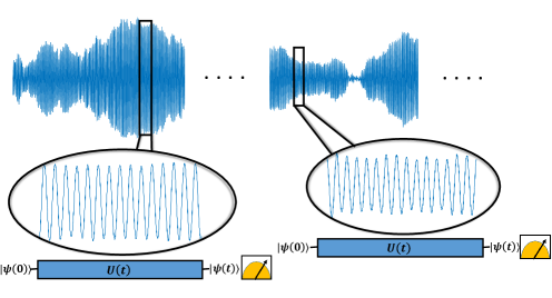
Consider now again the problem of spectral resolution, with the signal defined in eq. 1, and such that it suffers from shot-to-shot noise: in each measurement the frequencies are the same but the quadratures are random, i.e. Ai,Bisubscript𝐴𝑖subscript𝐵𝑖A_{i},\>B_{i} have a certain distribution. Specifically here we assume Ai,BiN(0,σ)similar-tosubscript𝐴𝑖subscript𝐵𝑖𝑁0𝜎A_{i},\>B_{i}\sim N\left(0,\sigma\right), and other noise models are addressed in supplementary note 11. This scenario is illustrated in fig. 2, and is relevant for different applications, such as communication protocols, spectrum analyzers and nano NMR (Balasubramanian et al. (2008); Gruber et al. (1997); Maze et al. (2008); Staudacher et al. (2013); Mamin et al. (2013); Müller et al. (2014); DeVience et al. (2015); Aslam et al. (2017); Bucher et al. (2018); Lovchinsky et al. (2016); Bar-Gill and Retzker (2017)), in particular when the time required to perform projective measurement is longer than the coherence time of the signal (this is the case with NV centers, due to the large number of iterations needed, and with trapped ions, where the re-cooling process might be longer than the coherence time of the qubit).

It is quite clear that the fluctuations of the quadratures remove the purity of the probe, which can give rise to superresolution states. Let us examine this.
Refer to caption
Figure 2: The problem of resolution without coherence. the quadratures of the signal in different measurements are random. The question we address is whether resolution is limited by the length of individual measurements.

Consider a standard Ramsey experiment, in which the probe is initialized in σxσysubscript𝜎𝑥subscript𝜎𝑦\sigma_{x}-\sigma_{y} plane, then rotated due to the signal and eventually measured in the initialization basis. Due to the fluctuations of the Hamiltonian, an averaging should be performed. Therefore the state of the probe is given by a density matrix:

ρ=p(Ai)p(Bi)|ψAi,BiψAi,Bi|𝑑Ai𝑑Bi,𝜌𝑝subscript𝐴𝑖𝑝subscript𝐵𝑖ketsubscript𝜓subscript𝐴𝑖subscript𝐵𝑖brasubscript𝜓subscript𝐴𝑖subscript𝐵𝑖differential-dsubscript𝐴𝑖differential-dsubscript𝐵𝑖\rho=\int p\left(A_{i}\right)p\left(B_{i}\right)|\psi_{A_{i},B_{i}}\rangle\langle\psi_{A_{i},B_{i}}|\;dA_{i}\>dB_{i}, (5)

where |ψAi,Biketsubscript𝜓subscript𝐴𝑖subscript𝐵𝑖|\psi_{A_{i},B_{i}}\rangle is the state given a single realization of Ai,Bi.subscript𝐴𝑖subscript𝐵𝑖A_{i},B_{i}. Note that since the fluctuations are identical:

ρ(ωr)=ρ(ωr)dρdωr=0(ωr=0).𝜌subscript𝜔r𝜌subscript𝜔r𝑑𝜌𝑑subscript𝜔r0subscript𝜔r0\rho\left(\omega_{\mathrm{r}}\right)=\rho\left(-\omega_{\mathrm{r}}\right)\Rightarrow\frac{d\rho}{d\omega_{\mathrm{r}}}=0\,\left(\omega_{\mathrm{r}}=0\right). (6)

Once again, control on the probe does not change this symmetry, hence superresolution can be achieved only if the condition presented above is satisfied: projection noise has to be nullified. It is therefore desirable to find a measurement scheme that nullifies the projection noise. It is simple to see that this can be obtained if ϕAi,Bi=0(Ai,Bi),subscriptitalic-ϕsubscript𝐴𝑖subscript𝐵𝑖0for-allsubscript𝐴𝑖subscript𝐵𝑖\phi_{A_{i},B_{i}}=0\>\left(\forall A_{i},B_{i}\right), where ϕAi,Bisubscriptitalic-ϕsubscript𝐴𝑖subscript𝐵𝑖\phi_{A_{i},B_{i}} is the phase accumulated by the sensor (defined as half the rotation angle in the Bloch sphere) per realization, since this implies a vanishing transition probability.

Our claim is therefore: Given the above noise model, there exist measurement schemes that satisfy the superresolution condition and thus achieve Ir>0.subscript𝐼r0I_{\mathrm{r}}>0. To see that such methods exist, observe that the phase accumulated by the sensor given the Hamiltonian in Eq. 1 (when no control is applied) reads:

ϕAi,Bi=𝑖Aiωisin(ωit)+Biωi(1cos(ωit)).subscriptitalic-ϕsubscript𝐴𝑖subscript𝐵𝑖𝑖subscript𝐴𝑖subscript𝜔𝑖subscript𝜔𝑖𝑡subscript𝐵𝑖subscript𝜔𝑖1subscript𝜔𝑖𝑡\phi_{A_{i},B_{i}}=\underset{i}{\sum}\frac{A_{i}}{\omega_{i}}\sin\left(\omega_{i}t\right)+\frac{B_{i}}{\omega_{i}}\left(1-\cos\left(\omega_{i}t\right)\right). (7)

Note that given this time evolution the density matrix of the sensor is diagonal in the initialization basis with eigenvalues p, 1p,𝑝1𝑝p,\,1-p, where p𝑝p is the average transition probability: p=sin(ϕAi,Bi)2Ai,Bi.p=\langle\sin\left(\phi_{A_{i},B_{i}}\right)^{2}\rangle_{A_{i},B_{i}}. Hence the superresolution condition boils down to pωr2.similar-to𝑝superscriptsubscript𝜔r2p\sim\omega_{\mathrm{r}}^{2}. This indeed can be satisfied by simply tuning t𝑡t such that ωst=2πn,subscript𝜔s𝑡2𝜋𝑛\omega_{\mathrm{s}}t=2\pi n, where n𝑛n is a non-zero integer. With this tuning ϕAi,Bi=0subscriptitalic-ϕsubscript𝐴𝑖subscript𝐵𝑖0\phi_{A_{i},B_{i}}=0 (for ωr=0subscript𝜔r0\omega_{\mathrm{r}}=0), and more specifically :

ϕAi,Bi(A1A2)ωsωrtp2σ2ωs2ωr2t2,subscriptitalic-ϕsubscript𝐴𝑖subscript𝐵𝑖subscript𝐴1subscript𝐴2subscript𝜔ssubscript𝜔r𝑡𝑝2superscript𝜎2superscriptsubscript𝜔s2superscriptsubscript𝜔r2superscript𝑡2\phi_{A_{i},B_{i}}\approx\frac{\left(A_{1}-A_{2}\right)}{\omega_{\mathrm{s}}}\omega_{\mathrm{r}}t\rightarrow p\approx\frac{2\sigma^{2}}{\omega_{\mathrm{s}}^{2}}\omega_{\mathrm{r}}^{2}t^{2}, (8)

Hence the superresolution condition is satisfied and the FI reads:

Ir=8σ2t2ωs2.subscript𝐼r8superscript𝜎2superscript𝑡2superscriptsubscript𝜔s2I_{\mathrm{r}}=\frac{8\sigma^{2}t^{2}}{\omega_{\mathrm{s}}^{2}}. (9)

So nullifying the projection noise indeed cancels the vanishing derivative and a finite Irsubscript𝐼rI_{\mathrm{r}} is achieved.

The obtained FI can be still quite poor and far from optimal. Note that it goes as 1/n2,1superscript𝑛21/n^{2}, where n𝑛n is the number of periods completed during the measurement. If n𝑛n is large, then this factor of 1n21superscript𝑛2\frac{1}{n^{2}} can be significant. A much better FI can be achieved by applying a suitable control: πlimit-from𝜋\pi-pulses which effectively change the frequency of oscillations, and reduce n𝑛n to 111 Kotler et al. (2011); Schmitt et al. (2017); Boss et al. (2017); Naghiloo et al. (2017):

Given an original Hamiltonian of H=[Asin(ωt)+Bcos(ωt)]σz,𝐻delimited-[]𝐴𝜔𝑡𝐵𝜔𝑡subscript𝜎𝑧H=\left[A\sin\left(\omega t\right)+B\cos\left(\omega t\right)\right]\sigma_{z}, applying πlimit-from𝜋\pi-pulses in a frequency of ω+δ𝜔𝛿\omega+\delta (namely a πlimit-from𝜋\pi-pulse is applied every πω+δ,𝜋𝜔𝛿\frac{\pi}{\omega+\delta}, δ𝛿\delta is referred to as detuning) on the probe yields the following effective Hamiltonian (see methods for a derivation):

Heff=tan(π2(1+δω))(δω)[Asin(δt)+Bcos(δt)]σz.subscript𝐻eff𝜋21𝛿𝜔𝛿𝜔delimited-[]𝐴𝛿𝑡𝐵𝛿𝑡subscript𝜎𝑧H_{\text{eff}}=\tan\left(\frac{\pi}{2\left(1+\frac{\delta}{\omega}\right)}\right)\left(\frac{\delta}{\omega}\right)\left[A\sin\left(\delta t\right)+B\cos\left(\delta t\right)\right]\sigma_{z}. (10)

Hence the πlimit-from𝜋\pi-pulses effectively change the frequency of the Hamiltonian from ω𝜔\omega to δ𝛿\delta (with a prefactor of tan(π2(1+δω))(δω)𝜋21𝛿𝜔𝛿𝜔\tan\left(\frac{\pi}{2\left(1+\frac{\delta}{\omega}\right)}\right)\left(\frac{\delta}{\omega}\right) added to the amplitude). Since we aim to reduce the frequency of oscillations, we focus on the limit of δω,much-less-than𝛿𝜔\delta\ll\omega, in which tan(π2(1+δω))(δω)2π,𝜋21𝛿𝜔𝛿𝜔2𝜋\tan\left(\frac{\pi}{2\left(1+\frac{\delta}{\omega}\right)}\right)\left(\frac{\delta}{\omega}\right)\approx\frac{2}{\pi}, and thus:

Heff2π[Asin(δt)+Bcos(δt)]σz.subscript𝐻eff2𝜋delimited-[]𝐴𝛿𝑡𝐵𝛿𝑡subscript𝜎𝑧H_{\text{eff}}\approx\frac{2}{\pi}\left[A\sin\left(\delta t\right)+B\cos\left(\delta t\right)\right]\sigma_{z}. (11)

When dealing with a signal that consists of two frequencies (ω1,ω2subscript𝜔1subscript𝜔2\omega_{1},\omega_{2}), the effective Hamiltonian becomes:

Heff𝑖2π[Aisin(δit)+Bicos(δit)]σz.subscript𝐻eff𝑖2𝜋delimited-[]subscript𝐴𝑖subscript𝛿𝑖𝑡subscript𝐵𝑖subscript𝛿𝑖𝑡subscript𝜎𝑧H_{\text{eff}}\approx\underset{i}{\sum}\frac{2}{\pi}\left[A_{i}\sin\left(\delta_{i}t\right)+B_{i}\cos\left(\delta_{i}t\right)\right]\sigma_{z}. (12)

Hence due to the control the central frequency is shifted to δs=δ1+δ22,subscript𝛿ssubscript𝛿1subscript𝛿22\delta_{\mathrm{s}}=\frac{\delta_{1}+\delta_{2}}{2}, and the relative frequency simply changes sign: δr=ωr.subscript𝛿rsubscript𝜔r\delta_{\mathrm{r}}=-\omega_{\mathrm{r}}. The condition of vanishing p𝑝p becomes: δst=±2πn,subscript𝛿s𝑡plus-or-minus2𝜋𝑛\delta_{\mathrm{s}}t=\pm 2\pi n, such that the optimal strategy is setting δst=±2π.subscript𝛿s𝑡plus-or-minus2𝜋\delta_{\mathrm{s}}t=\pm 2\pi. Therefore with these (optimal) values of δssubscript𝛿s\delta_{\mathrm{s}} the FI reads:

Ir(2π)28σ2t2δs2=8σ2t4π4.subscript𝐼rsuperscript2𝜋28superscript𝜎2superscript𝑡2superscriptsubscript𝛿s28superscript𝜎2superscript𝑡4superscript𝜋4I_{\mathrm{r}}\approx\left(\frac{2}{\pi}\right)^{2}\frac{8\sigma^{2}t^{2}}{\delta_{\mathrm{s}}^{2}}=\frac{8\sigma^{2}t^{4}}{\pi^{4}}. (13)

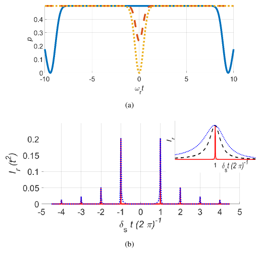
Observe that the scaling of Irsubscript𝐼rI_{\mathrm{r}} is optimal (goes as σ2t4superscript𝜎2superscript𝑡4\sigma^{2}t^{4}) Pang and Jordan (2017, 2017); Schmitt et al. (2017); Jordan (2017); Yang et al. (2017); Gefen et al. (2017); Naghiloo et al. (2017); however it is unknown whether this is the best achievable FI (see extended discussion in supplementary note 6). The probabilities and the FI for different detunings are presented in fig. 3. Note that clear resonance peaks of the FI are observed for δst=±2πn,subscript𝛿s𝑡plus-or-minus2𝜋𝑛\delta_{\mathrm{s}}t=\pm 2\pi n, any other values of detuning lead to a vanishing FI.
Refer to caption
Figure 3: Probability and Fisher information analysis (a) Average transition probability (p𝑝p) as a function of ωrtsubscript𝜔r𝑡\omega_{\mathrm{r}}t for different values of δssubscript𝛿s\delta_{\rm{s}}: δst=πsubscript𝛿s𝑡𝜋\delta_{\rm{s}}t=\pi (blue, solid line), δst=1.8πsubscript𝛿s𝑡1.8𝜋\delta_{\rm{s}}t=1.8\pi (orange, dashed line) and δst=2πsubscript𝛿s𝑡2𝜋\delta_{\rm{s}}t=2\pi (dotted,yellow line). For every δs,subscript𝛿s\delta_{\rm{s}}, dpdωr=0𝑑𝑝𝑑subscript𝜔r0\frac{dp}{d\omega_{\mathrm{r}}}=0 for ωr=0.subscript𝜔r0\omega_{\mathrm{r}}=0. Hence a finite Irsubscript𝐼rI_{\mathrm{r}} can be achieved only if p=0.𝑝0p=0. This requirement is fulfilled when δst=2πn.subscript𝛿s𝑡2𝜋𝑛\delta_{\rm{s}}t=2\pi n. (b) FI about ωrsubscript𝜔r\omega_{\mathrm{r}} (Irsubscript𝐼rI_{\mathrm{r}}) as a function of δst.subscript𝛿s𝑡\delta_{\rm{s}}t. Clear peaks can be observed whenever δst=2πn.subscript𝛿s𝑡2𝜋𝑛\delta_{\rm{s}}t=2\pi n. The width of the peaks is illustrated in the inset: for ωr=0,subscript𝜔r0\omega_{\mathrm{r}}=0, the width vanishes; however finite ωrsubscript𝜔r\omega_{\mathrm{r}} leads to a finite width (given ωrt1much-less-thansubscript𝜔r𝑡1\omega_{\mathrm{r}}t\ll 1 this width goes as ωrsubscript𝜔r\omega_{\mathrm{r}}, see section .3). For this illustration: ωrt=0.001subscript𝜔r𝑡0.001\omega_{\mathrm{r}}t=0.001 (red, solid line), ωrt=0.05subscript𝜔r𝑡0.05\omega_{\mathrm{r}}t=0.05 (black, dashed line),ωrt=0.1subscript𝜔r𝑡0.1\omega_{\mathrm{r}}t=0.1 (blue, dotted line).

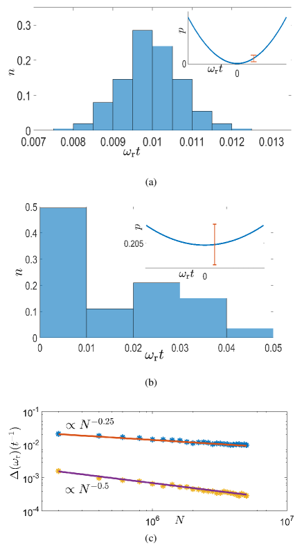
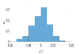
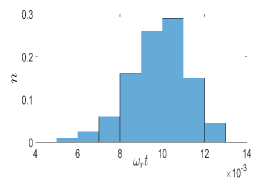
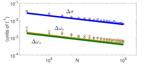
We tested this method numerically by generating data of two frequency signal (with the corresponding noise model) and performing a Maximum-Likelihood estimation (MLE) to find ωr.subscript𝜔r\omega_{\rm{r}}. Some of the results are shown in fig. 4. It can be seen that by choosing a detuning such that δst=2π,subscript𝛿s𝑡2𝜋\delta_{\mathrm{s}}t=2\pi, ωrsubscript𝜔r\omega_{\mathrm{r}} can be estimated efficiently and the frequencies are resolved. As shown in fig. 4, the standard deviation matches the theoretical expectation: Δωr=1IrN.Δsubscript𝜔r1subscript𝐼r𝑁\Delta\omega_{\mathrm{r}}=\frac{1}{\sqrt{I_{\rm{r}}N}}. By utilizing this control method the number of measurements (N𝑁N) needed to achieve resolution is Np1=π42σ2ωr2t4.much-greater-than𝑁superscript𝑝1superscript𝜋42superscript𝜎2superscriptsubscript𝜔r2superscript𝑡4N\gg p^{-1}=\frac{\pi^{4}}{2\sigma^{2}\omega_{\rm{r}}^{2}t^{4}}. Taking for example values which are well beyond the resolution limit such as ωrt=0.01,σt=1,formulae-sequencesubscript𝜔r𝑡0.01𝜎𝑡1\omega_{\rm{r}}t=0.01,\>\sigma t=1, resolution is achieved for N5105.much-greater-than𝑁5superscript105N\gg 5\cdot 10^{5}. If the chosen detuning does not satisfy one of theses conditions (δst=2πnsubscript𝛿𝑠𝑡2𝜋𝑛\delta_{s}t=2\pi n) we expect to observe a divergence in the variance. We used MLE for this case as well. Note that the fact that the FI vanishes does not mean that no information about ωrsubscript𝜔r\omega_{\rm{r}} is obtained, information is in fact obtained from the second derivative. The estimator becomes biased and the standard deviation reads: Δωr=(p(1p))0.252pωr2N0.25,Δsubscript𝜔rsuperscript𝑝1𝑝0.25superscript2𝑝superscriptsubscript𝜔r2superscript𝑁0.25\Delta\omega_{\rm{r}}=\frac{\left(p\left(1-p\right)\right)^{0.25}}{\sqrt{\frac{\partial^{2}p}{\partial\omega_{\rm{r}}^{2}}}N^{0.25}}, see fig. 4. The fact that the standard deviation is proportional to N0.25superscript𝑁0.25N^{-0.25} (as opposed to the standard scaling of N0.5superscript𝑁0.5N^{-0.5}) is a manifestation of the divergence. The resolution condition in this case is thus: Np(1p)(2pωr2)2ωr4.much-greater-than𝑁𝑝1𝑝superscriptsuperscript2𝑝superscriptsubscript𝜔r22superscriptsubscript𝜔r4N\gg\frac{p\left(1-p\right)}{\left(\frac{\partial^{2}p}{\partial\omega_{\rm{r}}^{2}}\right)^{2}\omega_{\rm{r}}^{4}}. Considering the same example as previously (ωrt=0.01,σt=1formulae-sequencesubscript𝜔r𝑡0.01𝜎𝑡1\omega_{\rm{r}}t=0.01,\>\sigma t=1) but with off-resonance detuning (δst=1.8π)subscript𝛿𝑠𝑡1.8𝜋\left(\delta_{s}t=1.8\pi\right), the number of measurements required for resolution is N108;much-greater-than𝑁superscript108N\gg 10^{8}; hence a difference of almost three orders of magnitude.

This method can be understood in the following simple and intuitive way: If there is only a single frequency and δs=2πtsubscript𝛿𝑠2𝜋𝑡\delta_{s}=\frac{2\pi}{t} then pa=0,subscript𝑝𝑎0p_{a}=0, hence no transitions should occur, whereas a finite (small) ωrsubscript𝜔r\omega_{\rm{r}} should lead to a small transition probability (p)𝑝\left(p\right), such that transitions will be observed after 1p=π42σ2ωr2t41𝑝superscript𝜋42superscript𝜎2superscriptsubscript𝜔r2superscript𝑡4\frac{1}{p}=\frac{\pi^{4}}{2\sigma^{2}\omega_{\rm{r}}^{2}t^{4}} measurements.

Refer to caption
Figure 4: Estimation analysis. Maximum likelihood estimation of ωrsubscript𝜔r\omega_{\rm{r}} (beyond the resolution limit; i.e. ωrt1much-less-thansubscript𝜔r𝑡1\omega_{\rm{r}}t\ll 1) with different control methods. (a)+(b) Histogram of the estimated ωrsubscript𝜔r\omega_{\rm{r}} for the optimal control method: δst=2π,subscript𝛿𝑠𝑡2𝜋\delta_{s}t=2\pi, compared to the histogram obtained slightly off the resonance: δst=1.8π.subscript𝛿𝑠𝑡1.8𝜋\delta_{s}t=1.8\pi. When resonance is achieved, the two frequencies are clearly resolved (Δωr<110ωrΔsubscript𝜔r110subscript𝜔r\Delta\omega_{\rm{r}}<\frac{1}{10}\omega_{\rm{r}}), while off the resonance they are not resolvable (Δωr>ωrΔsubscript𝜔rsubscript𝜔r\Delta\omega_{\rm{r}}>\omega_{\rm{r}}). Note that off resonance, the standard deviation is too large; hence the probability cannot be distinguished from p(ωr=0)𝑝subscript𝜔r0p\left(\omega_{\rm{r}}=0\right) (see insets). For both plots N=106,σt=5,ωrt=0.01.formulae-sequence𝑁superscript106formulae-sequence𝜎𝑡5subscript𝜔r𝑡0.01N=10^{6},\sigma t=5,\omega_{\rm{r}}t=0.01. (c) The RMSE (root mean square error) as a function of N𝑁N for both control methods. For δst=2πsubscript𝛿𝑠𝑡2𝜋\delta_{s}t=2\pi the RMSE goes as (NIr)0.5superscript𝑁subscript𝐼r0.5\left(NI_{\rm{r}}\right)^{-0.5} as expected. Off the resonance (δst=1.8πsubscript𝛿𝑠𝑡1.8𝜋\delta_{s}t=1.8\pi) the FI vanishes and the RMSE goes as N0.25superscript𝑁0.25N^{-0.25} (the estimation is biased).

.3 Limitations and imperfections

The method, as analyzed so far, assumes knowledge of all the other parameters (σ𝜎\sigma and ωssubscript𝜔s\omega_{\rm{s}}), coherence of the signal and the probe during the measurement period, and measurements with unit fidelity. In this section we analyze each one of these assumptions. The first one to be analyzed is the main caveat of the method: the requirement of coherence during the measurement period.

This method relies on the ability to nullify projection noise, in particular on the fact that for ωr=0subscript𝜔r0\omega_{\rm{r}}=0 the state can become pure. However this is achieved only for a signal which is perfectly coherent during each measurement. Fluctuations of the signal during the measurement period inflict a limitation, as in this case it is not possible to nullify the projection noise. Heuristically due to these fluctuations the transition probability includes an additional noise term (denoted as ϵitalic-ϵ\epsilon), such that it reads (for ωst=2πsubscript𝜔s𝑡2𝜋\omega_{\rm{s}}t=2\pi):

p=σ2t22π2ωr2t2+ϵ.𝑝superscript𝜎2superscript𝑡22superscript𝜋2superscriptsubscript𝜔r2superscript𝑡2italic-ϵp=\frac{\sigma^{2}t^{2}}{2\pi^{2}}\omega_{\mathrm{r}}^{2}t^{2}+\epsilon. (14)

This new term imposes a limitation: It is now impossible to nullify p,𝑝p, which implies that Ir0subscript𝐼r0I_{\mathrm{r}}\rightarrow 0 as ωr0.subscript𝜔r0\omega_{\mathrm{r}}\rightarrow 0. The FI (for ωst=2π,ωrt1)formulae-sequencefor subscript𝜔s𝑡2𝜋much-less-thansubscript𝜔r𝑡1\left(\text{for }\omega_{\rm{s}}t=2\pi,\omega_{\rm{r}}t\ll 1\right) now reads:

Ir(σt)2(ωrt)2π4(ϵ+σ2t22π2ωr2t2),subscript𝐼rsuperscript𝜎𝑡2superscriptsubscript𝜔r𝑡2superscript𝜋4italic-ϵsuperscript𝜎2superscript𝑡22superscript𝜋2superscriptsubscript𝜔r2superscript𝑡2I_{{\rm{r}}}\approx\frac{\left(\sigma t\right)^{2}\left(\omega_{\rm{r}}t\right)^{2}}{\pi^{4}\left(\epsilon+\frac{\sigma^{2}t^{2}}{2\pi^{2}}\omega_{\rm{r}}^{2}t^{2}\right)}, (15)

this behavior is illustrated in fig. 5, and it can be observed that resolution can be achieved only for ωrt>ϵσt.subscript𝜔r𝑡italic-ϵ𝜎𝑡\omega_{\rm{r}}t>\frac{\sqrt{\epsilon}}{\sigma t}.

More specifically, assuming a realistic noise model: the quadratures undergo OU (Ornstein-Uhlenbeck) noise process (with variance σn2superscriptsubscript𝜎𝑛2\sigma_{n}^{2} and damping rate γ𝛾\gamma), the noise term reads (in leading order of (γt1)much-less-than𝛾𝑡1\left(\gamma t\ll 1\right), see supplementary note 8 ) ϵ=σn2t3π2.italic-ϵsuperscriptsubscript𝜎𝑛2superscript𝑡3superscript𝜋2\epsilon=\frac{\sigma_{n}^{2}t^{3}}{\pi^{2}}. When comparing ϵitalic-ϵ\epsilon to the original transition probability: σ2t22π2ωr2t2=σn2t24π2γωr2t2,superscript𝜎2superscript𝑡22superscript𝜋2superscriptsubscript𝜔r2superscript𝑡2superscriptsubscript𝜎𝑛2superscript𝑡24superscript𝜋2𝛾superscriptsubscript𝜔r2superscript𝑡2\sigma^{2}\frac{t^{2}}{2\pi^{2}}\omega_{\rm{r}}^{2}t^{2}=\frac{\sigma_{n}^{2}t^{2}}{4\pi^{2}\gamma}\omega_{\rm{r}}^{2}t^{2}, we get the Fourier limit: ωrγ>1.subscript𝜔r𝛾1\frac{\omega_{\rm{r}}}{\gamma}>1. We remark that whether one can remove this limitation is an open question. Therefore this method is relevant mainly for experimental scenarios with noise that is effectively shot to shot: small enough fluctuations during each measurement but no correlations between consecutive measurements. This is the case in many experimental settings, where the time separation between measurements is longer than the phase acquisition period due to long readout and preparation stages.

Quite similarly, dephasing of the probe also imposes a limitation. Taking into account a dephasing rate κ,𝜅\kappa, the transition probability reads: p=0.5(1exp((σt)2(ωrt)2π22κt)).𝑝0.51superscript𝜎𝑡2superscriptsubscript𝜔r𝑡2superscript𝜋22𝜅𝑡p=0.5\left(1-\exp\left(-\frac{\left(\sigma t\right)^{2}\left(\omega_{\rm{r}}t\right)^{2}}{\pi^{2}}-2\kappa t\right)\right). Hence resolution can be achieved only if ωrσ(κ2)1.much-greater-thansubscript𝜔r𝜎superscript𝜅21\frac{\omega_{\rm{r}}\sigma}{\left(\kappa^{2}\right)}\gg 1. Note that in order to retrieve the noiseless FI it is not enough to require κt1,much-less-than𝜅𝑡1\kappa t\ll 1, as there is also minimal time t>κ1/3σ2/3ωr2/3𝑡superscript𝜅13superscript𝜎23superscriptsubscript𝜔r23t>\frac{\kappa^{1/3}}{\sigma^{2/3}\omega_{\rm{r}}^{2/3}} (κt𝜅𝑡\kappa t should be smaller than (σt)2(ωrt)2superscript𝜎𝑡2superscriptsubscript𝜔r𝑡2\left(\sigma t\right)^{2}\left(\omega_{\rm{r}}t\right)^{2}). A detailed analysis of this limitation can be found in supplementary note 9.

We next address the consequences of imperfect measurements. The effect of imperfect measurements is similar to that of incoherence, therefore the measurement infidelity sets a resolution limit. We consider a model in which there are two different outcomes and there is a finite probability to get each outcome from both states (as is the case for the NV center Batalov et al. (2008)). Namely the probability of detecting an outcome that corresponds to the bright state is: p=(1ϵ)pb+ϵpd,𝑝1superscriptitalic-ϵsubscript𝑝𝑏superscriptitalic-ϵsubscript𝑝𝑑p=\left(1-\epsilon^{\prime}\right)p_{b}+\epsilon^{\prime}p_{d}, where pbsubscript𝑝𝑏p_{b} (pdsubscript𝑝𝑑p_{d}) denotes the probability of the bright (dark) state and then ϵsuperscriptitalic-ϵ\epsilon^{\prime} is the probability of wrong detection. Given this error probability we can observe that dpdωr=0𝑑𝑝𝑑subscript𝜔r0\frac{dp}{d\omega_{\mathrm{r}}}=0 (when ωr=0subscript𝜔r0\omega_{\mathrm{r}}=0) but it is impossible to nullify p𝑝p. This implies Ir0subscript𝐼r0I_{\rm{r}}\rightarrow 0 as ωr0.subscript𝜔r0\omega_{\mathrm{r}}\rightarrow 0. Therefore taking ϵ1much-less-thansuperscriptitalic-ϵ1\epsilon^{\prime}\ll 1 (and ωrt1,ωst=2πformulae-sequencemuch-less-thansubscript𝜔r𝑡1subscript𝜔s𝑡2𝜋\omega_{\mathrm{r}}t\ll 1,\omega_{\rm{s}}t=2\pi) we get the same expression as in eq. 14 (with a noise term of ϵsuperscriptitalic-ϵ\epsilon^{\prime}): pσ2T22π2ωr2T2+ϵ.𝑝superscript𝜎2superscript𝑇22superscript𝜋2superscriptsubscript𝜔r2superscript𝑇2superscriptitalic-ϵp\approx\frac{\sigma^{2}T^{2}}{2\pi^{2}}\omega_{\mathrm{r}}^{2}T^{2}+\epsilon^{\prime}. Hence resolution limit is given by: ωrT>ϵσTsubscript𝜔r𝑇superscriptitalic-ϵ𝜎𝑇\omega_{\mathrm{r}}T>\frac{\sqrt{\epsilon^{\prime}}}{\sigma T} (see fig. 5).

Let us now address the multivariable estimation protocol. In any realistic scenario σ𝜎\sigma and ωssubscript𝜔s\omega_{\rm{s}} are unknown. Since the estimation protocol of ωrsubscript𝜔r\omega_{\mathrm{r}} depends on knowledge of ωssubscript𝜔s\omega_{\rm{s}} a preliminary estimation of ωssubscript𝜔s\omega_{\rm{s}} must be performed (quite analogously to the preliminary estimation of the centroid in quantum resolution methods for optical imaging Parniak et al. (2018); Nair and Tsang (2016b) ). This can be done using the traditional method Pham et al. (2016): Applying π𝜋\pi-pulses in different frequencies and fitting the transition probability as a function of the pulses frequency (see supplementary note 7). This should provide a good estimation of σ,ωs,𝜎subscript𝜔s\sigma,\omega_{\rm{s}}, but not a good enough estimation of ωrsubscript𝜔r\omega_{\rm{r}} (unless by chance we hit close enough to a resonance frequency). Once a good enough estimation of ωssubscript𝜔s\omega_{\rm{s}} is obtained we can apply the required control (δst=2πsubscript𝛿𝑠𝑡2𝜋\delta_{s}t=2\pi). To understand what is a good enough estimation of ωssubscript𝜔s\omega_{\rm{s}} observe that for small enough ωrt,(δst2π)subscript𝜔r𝑡subscript𝛿𝑠𝑡2𝜋\omega_{\rm{r}}t,\left(\delta_{s}t-2\pi\right): Ir=8σ2t4π4ωr2ωr2+(δs2π/t)2,subscript𝐼r8superscript𝜎2superscript𝑡4superscript𝜋4superscriptsubscript𝜔r2superscriptsubscript𝜔r2superscriptsubscript𝛿𝑠2𝜋𝑡2I_{\rm{r}}=\frac{8\sigma^{2}t^{4}}{\pi^{4}}\frac{\omega_{\rm{r}}^{2}}{\omega_{\rm{r}}^{2}+\left(\delta_{s}-2\pi/t\right)^{2}}, hence the width of the resonance peak (in δstsubscript𝛿𝑠𝑡\delta_{s}t) goes as ωrt.subscript𝜔r𝑡\omega_{\rm{r}}t. Therefore once ΔωsΔsubscript𝜔s\Delta{\omega_{\rm{s}}} is comparable to ωrsubscript𝜔r\omega_{\rm{r}} this method works despite the small detuning.

Observe that now a multivariate estimation should be performed, which means that at least three different measurements are needed; each measurement in a detuning that is optimal for a different parameter. Numerical results and further analysis are presented in supplementary note 7.
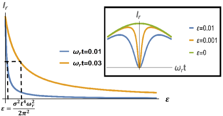
Refer to caption
Figure 5: The effect of noise. Irsubscript𝐼rI_{\mathrm{r}} as a function of ϵitalic-ϵ\epsilon (a general noise term in the measurement, see eq. 14) for different values of ωr.subscript𝜔r\omega_{\mathrm{r}}. Irsubscript𝐼rI_{\mathrm{r}} drops to half the maximal value for ϵ=(σt)2(ωrt)22π2,italic-ϵsuperscript𝜎𝑡2superscriptsubscript𝜔r𝑡22superscript𝜋2\epsilon=\frac{\left(\sigma t\right)^{2}\left(\omega_{\mathrm{r}}t\right)^{2}}{2\pi^{2}}, which means that the maximal ϵitalic-ϵ\epsilon for which resolution can be achieved goes as (σt)2(ωrt)2.superscript𝜎𝑡2superscriptsubscript𝜔r𝑡2\left(\sigma t\right)^{2}\left(\omega_{\mathrm{r}}t\right)^{2}. In the inset: Irsubscript𝐼rI_{\mathrm{r}} as a function of ωrsubscript𝜔r\omega_{\mathrm{r}} for different ϵ.italic-ϵ\epsilon.

.4 Additional applications: quantum resolution methods for sampling

Superresolution with quantum Fourier transform (QFT) : Consider the signal (Hamiltonian) in eq. 1, if the coherence time of the signal is relatively long, its spectrum can be found by sampling it (where sampling means Ramsey measurements of the probe in different times). Several recent experiments implemented this scheme Schmitt et al. (2017); Boss et al. (2017); Glenn et al. (2018). The straightforward (and natural) way to analyze this data is by fitting the power spectrum of the measurement outcomes, however it was shown in Rotem et al. (2019) that this method suffers from a resolution limit. The reason is again that the (average) power spectrum is symmetric with respect to ωr,subscript𝜔r\omega_{\rm{r}}, yet the measurement noise does not vanish. We point out here that this limit can be eliminated if instead of classical Fourier transform, one uses a quantum Fourier transform. In more detail: a phase of ϕjτ𝑖(Aicos(ωitj)+Bisin(ωitj))subscriptitalic-ϕ𝑗𝜏𝑖subscript𝐴𝑖subscript𝜔𝑖subscript𝑡𝑗subscript𝐵𝑖subscript𝜔𝑖subscript𝑡𝑗\phi_{j}\approx\tau\underset{i}{\sum}\left(A_{i}\cos\left(\omega_{i}t_{j}\right)+B_{i}\sin\left(\omega_{i}t_{j}\right)\right) is accumulated by the probe in each measurement (where τ𝜏\tau is the length of each measurement). The idea is that instead of measuring the probe after each phase acquisition, we can map the phases to memory qubits to form the state: |ψ=1Nj=1𝑁eiϕj|j,ket𝜓1𝑁𝑗1𝑁superscript𝑒𝑖subscriptitalic-ϕ𝑗ket𝑗|\psi\rangle=\frac{1}{\sqrt{N}}\underset{j=1}{\overset{N}{\sum}}e^{i\phi_{j}}|j\rangle, and then measure in the Fourier basis. With the appropriate choice of total sampling time (T=m2πωs𝑇𝑚2𝜋subscript𝜔sT=m\frac{2\pi}{\omega_{\rm{s}}}, for an integer m𝑚m) and measurement length (τ=2πnωs,𝜏2𝜋𝑛subscript𝜔s\tau=\frac{2\pi}{n\omega_{\rm{s}}}, for an integer n𝑛n), the only states in the Fourier basis that can be measured are harmonics of ωssubscript𝜔s\omega_{\rm{s}} (for ωr=0subscript𝜔r0\omega_{\mathrm{r}}=0), hence vanishing projection noise of all the others outcomes. The probability to measure the other frequencies, for ωrT1,much-less-thansubscript𝜔r𝑇1\omega_{\mathrm{r}}T\ll 1, is 16ωr2T2(στ)2absent16superscriptsubscript𝜔r2superscript𝑇2superscript𝜎𝜏2\approx\frac{1}{6}\omega_{\mathrm{r}}^{2}T^{2}\left(\sigma\tau\right)^{2} (see supplementary note 10), therefore Ir=23(στ)2T2subscript𝐼r23superscript𝜎𝜏2superscript𝑇2I_{\mathrm{r}}=\frac{2}{3}\left(\sigma\tau\right)^{2}T^{2} for ωr=0.subscript𝜔r0\omega_{\mathrm{r}}=0. We thus get a non vanishing FI, and it can be shown that for any model in which the phases are uniformly distributed, the optimal measurement basis is indeed the Fourier basis.

A different method for the same problem is superresolution with correlation spectroscopy: The Hamiltonian is the same, but now perform two measurements and correlate between them using a single memory qubit, namely the state of the memory qubit after the two phase accumulation periods is 12(|0+ei(ϕ1ϕ2)|1),12ket0superscript𝑒𝑖subscriptitalic-ϕ1subscriptitalic-ϕ2ket1\frac{1}{\sqrt{2}}\left(|0\rangle+e^{i\left(\phi_{1}-\phi_{2}\right)}|1\rangle\right), where ϕjsubscriptitalic-ϕ𝑗\phi_{j} is the phase accumulated in the j𝑗jth period. It is simple to see that by choosing the period between measurements to be T=2πωsn,𝑇2𝜋subscript𝜔s𝑛T=\frac{2\pi}{\omega_{\rm{s}}}n, and measuring in the initialization basis the transition probability is p(B1B2)2τ2ωr2T2.𝑝delimited-⟨⟩superscriptsubscript𝐵1subscript𝐵22superscript𝜏2superscriptsubscript𝜔r2superscript𝑇2p\approx\langle\left(B_{1}-B_{2}\right)^{2}\rangle\tau^{2}\omega_{\rm{r}}^{2}T^{2}. Therefore a non-vanishing FI is achieved: Ir=4(B1B2)2τ2T2=8(στ)2T2.subscript𝐼r4delimited-⟨⟩superscriptsubscript𝐵1subscript𝐵22superscript𝜏2superscript𝑇28superscript𝜎𝜏2superscript𝑇2I_{\rm{r}}=4\langle\left(B_{1}-B_{2}\right)^{2}\rangle\tau^{2}T^{2}=8\left(\sigma\tau\right)^{2}T^{2}.

Discussion

We presented methods that are capable of resolving frequencies beyond the resolution limits (ωrt1much-less-thansubscript𝜔r𝑡1\omega_{\rm{r}}t\ll 1) in quantum spectroscopy. Those methods are special cases of a general superresolution criterion: one can overcome the vanishing derivative by making the projection noise vanish at the same rate. The main method that was analyzed (resolution without coherence) is applicable with state of the art experimental capabilities and does not require involved numerical analysis.

It would be interesting to inquire whether similar ideas are useful to other resolution problems, such as resolving the locations and the frequencies of single neighboring spins.

The methods presented above are not perfect, they are limited by the noise of the signal and the dephasing of the probe, whether one can overcome these limitations is an open question.

Methods

Derivation of density matrix and probabilities

Given a noise model on the amplitudes, the quantum state of the probe is described by the following density matrix:

ρ=|ψψ|p(𝑨,𝑩)𝑑𝑨𝑑𝑩.𝜌ket𝜓bra𝜓𝑝𝑨𝑩differential-d𝑨differential-d𝑩\rho=\int|\psi\rangle\langle\psi|\>p\left(\bm{A},\bm{B}\right)\>d\bm{A}\,d\bm{B}. (16)

Since the time evolution (with and without control) is described by the operator: U=cos(ϕ)𝟙isin(ϕ)σz,𝑈italic-ϕdouble-struck-𝟙𝑖italic-ϕsubscript𝜎𝑧U=\cos\left(\phi\right)\mathbb{1}-i\sin\left(\phi\right)\sigma_{z}, ρ𝜌\rho reads:

ρ=[cos(ϕ)2ρ0+sin(ϕ)2σzρ0σzi2sin(2ϕ)[σz,ρ0]]p(𝑨,𝑩)d𝑨d𝑩,\displaystyle\begin{split}&\rho=\int\left[\cos\left(\phi\right)^{2}\rho_{0}+\sin\left(\phi\right)^{2}\sigma_{z}\rho_{0}\sigma_{z}-\frac{i}{2}\sin\left(2\phi\right)\left[\sigma_{z},\rho_{0}\right]\right]\cdot\\ &p\left(\bm{A},\bm{B}\right)\>d\bm{A}\,d\bm{B},\end{split} (17)

where ρ0subscript𝜌0\rho_{0} is the initial state. With the relevant noise model (Ai,BiN(0,σ)similar-tosubscript𝐴𝑖subscript𝐵𝑖𝑁0𝜎A_{i},B_{i}\sim N\left(0,\sigma\right)) it can be seen that the terms going as sin(2ϕ)2italic-ϕ\sin\left(2\phi\right) vanish, leading to:

ρ=(1p)ρ0+pσzρ0σz,𝜌1𝑝subscript𝜌0𝑝subscript𝜎𝑧subscript𝜌0subscript𝜎𝑧\rho=\left(1-p\right)\rho_{0}+p\sigma_{z}\rho_{0}\sigma_{z}, (18)

where p𝑝p is the (averaged) transition probability: sin(ϕ)2p(𝑨,𝑩)d𝑨d𝑩.\int\sin\left(\phi\right)^{2}p\left(\bm{A},\bm{B}\right)\>d\bm{A}\,d\bm{B}. Taking ϕ=iAisin(δit)δi+Bi1cos(δit)δi,italic-ϕsubscript𝑖subscript𝐴𝑖subscript𝛿𝑖𝑡subscript𝛿𝑖subscript𝐵𝑖1subscript𝛿𝑖𝑡subscript𝛿𝑖\phi=\sum_{i}A_{i}\frac{\sin\left(\delta_{i}t\right)}{\delta_{i}}+B_{i}\frac{1-\cos\left(\delta_{i}t\right)}{\delta_{i}}, a simple calculation yields:

p=0.5(1exp(8iσ2δi2sin2(δit2))).𝑝0.518subscript𝑖superscript𝜎2superscriptsubscript𝛿𝑖2superscript2subscript𝛿𝑖𝑡2p=0.5\left(1-\exp\left(-8\sum_{i}\frac{\sigma^{2}}{\delta_{i}^{2}}\sin^{2}\left(\frac{\delta_{i}t}{2}\right)\right)\right). (19)

Note that this expression coincides with eq. 8 for δst=2π,subscript𝛿s𝑡2𝜋\delta_{\rm{s}}t=2\pi, ωrt1.much-less-thansubscript𝜔r𝑡1\omega_{\mathrm{r}}t\ll 1. The optimal initial state would be ρ0=|xx|\rho_{0}=|\uparrow_{x}\rangle\langle\uparrow_{x}| (or any other pure state in the XY𝑋𝑌X-Y plane), leading to ρ=(1p)|xx|+p|xx|.\rho=\left(1-p\right)|\uparrow_{x}\rangle\langle\uparrow_{x}|+p|\downarrow_{x}\rangle\langle\downarrow_{x}|. The QFI (about ωrsubscript𝜔r\omega_{\mathrm{r}}) of ρ𝜌\rho is thus: (dpdωr)2p(1p),superscript𝑑𝑝𝑑subscript𝜔r2𝑝1𝑝\frac{\left(\frac{dp}{d\omega_{\mathrm{r}}}\right)^{2}}{p\left(1-p\right)}, which is the expression of Irsubscript𝐼rI_{\mathrm{r}} mentioned in the main text.

Effective Hamiltonian derivation

In this section we derive the effective Hamiltonian that appears in the main text. Given a Hamiltonian: H=[Asin(ωt)+Bcos(ωt)]σz,𝐻delimited-[]𝐴𝜔𝑡𝐵𝜔𝑡subscript𝜎𝑧H=\left[A\sin\left(\omega t\right)+B\cos\left(\omega t\right)\right]\sigma_{z}, and π𝜋\pi-pulses that are applied every τ,𝜏\tau, the Hamiltonian in the interaction picture of these pulses is:

H=[Asin(ωt)+Bcos(ωt)]h(t)σz,𝐻delimited-[]𝐴𝜔𝑡𝐵𝜔𝑡𝑡subscript𝜎𝑧H=\left[A\sin\left(\omega t\right)+B\cos\left(\omega t\right)\right]h\left(t\right)\sigma_{z}, (20)

where h(t)𝑡h\left(t\right) is the square wave function. Note that the phase accumulated by the sensor (denoted as ϕ,italic-ϕ\phi, and defined as half the rotation angle in Bloch sphere) in t=nτ𝑡𝑛𝜏t=n\tau is:

ϕ=AIm(Φ)+BRe(Φ)where:Φ=n=0N1nτ(n+1)τeiωt(1)n𝑑titalic-ϕ𝐴ImΦ𝐵ReΦwhere:Φ𝑛0𝑁1superscriptsubscript𝑛𝜏𝑛1𝜏superscript𝑒𝑖𝜔𝑡superscript1𝑛differential-d𝑡\displaystyle\begin{split}&\phi=A\>\text{Im}\left(\Phi\right)+B\>\text{Re}\left(\Phi\right)\;\text{where:}\\ &\Phi=\underset{n=0}{\overset{N-1}{\sum}}\int_{n\tau}^{\left(n+1\right)\tau}e^{i\omega t}\left(-1\right)^{n}\>dt\end{split} (21)

where Re (Im) denotes the real (imaginary) part. Therefore in order to find ϕitalic-ϕ\phi we need to calculate ΦΦ\Phi:

Φ=n=0N1eiωnτ(1)neiωτ1iω=n=0N1ein(ωτ+π)eiωτ1iω.Φ𝑛0𝑁1superscript𝑒𝑖𝜔𝑛𝜏superscript1𝑛superscript𝑒𝑖𝜔𝜏1𝑖𝜔𝑛0𝑁1superscript𝑒𝑖𝑛𝜔𝜏𝜋superscript𝑒𝑖𝜔𝜏1𝑖𝜔\Phi=\underset{n=0}{\overset{N-1}{\sum}}e^{i\omega n\tau}\left(-1\right)^{n}\frac{e^{i\omega\tau}-1}{i\omega}=\underset{n=0}{\overset{N-1}{\sum}}e^{in\left(\omega\tau+\pi\right)}\frac{e^{i\omega\tau}-1}{i\omega}. (22)

The calculation then proceeds as follows:

Φ=1eiN(ωτ+π)1+eiωτeiωτ1iω=2ieiN2(ωτ+π)sin(Nωτ2+Nπ2)sin(ωτ2)1cos(ωτ2)ω.Φ1superscript𝑒𝑖𝑁𝜔𝜏𝜋1superscript𝑒𝑖𝜔𝜏superscript𝑒𝑖𝜔𝜏1𝑖𝜔2𝑖superscript𝑒𝑖𝑁2𝜔𝜏𝜋𝑁𝜔𝜏2𝑁𝜋2𝜔𝜏21𝜔𝜏2𝜔\displaystyle\begin{split}&\Phi=\frac{1-e^{iN\left(\omega\tau+\pi\right)}}{1+e^{i\omega\tau}}\frac{e^{i\omega\tau}-1}{i\omega}=\\ &-2ie^{i\frac{N}{2}\left(\omega\tau+\pi\right)}\sin\left(N\frac{\omega\tau}{2}+N\frac{\pi}{2}\right)\sin\left(\omega\frac{\tau}{2}\right)\frac{1}{\cos\left(\frac{\omega\tau}{2}\right)\omega}.\end{split} (23)

Hence:

Re(Φ)=(1cos(ωt+Nπ))sin(ωτ2)cos(ωτ2)ω,Im(Φ)=sin(ωt+Nπ)sin(ωτ2)ωcos(ωτ2).formulae-sequenceReΦ1𝜔𝑡𝑁𝜋𝜔𝜏2𝜔𝜏2𝜔ImΦ𝜔𝑡𝑁𝜋𝜔𝜏2𝜔𝜔𝜏2\displaystyle\begin{split}&\text{Re}\left(\Phi\right)=\left(1-\cos\left(\omega t+N\pi\right)\right)\frac{\sin\left(\omega\frac{\tau}{2}\right)}{\cos\left(\omega\frac{\tau}{2}\right)\omega},\\ &\text{Im}\left(\Phi\right)=-\sin\left(\omega t+N\pi\right)\frac{\sin\left(\omega\frac{\tau}{2}\right)}{\omega\cos\left(\frac{\omega\tau}{2}\right)}.\end{split} (24)

Note that: ωt=ωNπω+δ=Nπδt,𝜔𝑡𝜔𝑁𝜋𝜔𝛿𝑁𝜋𝛿𝑡\omega t=\omega N\frac{\pi}{\omega+\delta}=N\pi-\delta t, therefore eq. 24 is simplified to:

Re(Φ)=(1cos(δt))tan(ωτ2)ω,Im(Φ)=sin(δt)tan(ωτ2)ω.formulae-sequenceReΦ1𝛿𝑡𝜔𝜏2𝜔ImΦ𝛿𝑡𝜔𝜏2𝜔\displaystyle\begin{split}&\text{Re}\left(\Phi\right)=\left(1-\cos\left(\delta t\right)\right)\frac{\tan\left(\omega\frac{\tau}{2}\right)}{\omega},\\ &\text{Im}\left(\Phi\right)=\sin\left(\delta t\right)\frac{\tan\left(\omega\frac{\tau}{2}\right)}{\omega}.\end{split} (25)

The accumulated phase,ϕitalic-ϕ\phi, thus reads:

ϕ=Asin(δt)tan(ωτ2)ω+B(1cos(δt))tan(ωτ2)ω.italic-ϕ𝐴𝛿𝑡𝜔𝜏2𝜔𝐵1𝛿𝑡𝜔𝜏2𝜔\phi=A\sin\left(\delta t\right)\frac{\tan\left(\omega\frac{\tau}{2}\right)}{\omega}+B\left(1-\cos\left(\delta t\right)\right)\frac{\tan\left(\omega\frac{\tau}{2}\right)}{\omega}. (26)

Observe that this exact phase is obtained by the following effective Hamiltonian (note that no approximation is used here):

Heff=tan(ωτ2)(δω)[Acos(δt)+Bsin(δt)]σz,subscript𝐻eff𝜔𝜏2𝛿𝜔delimited-[]𝐴𝛿𝑡𝐵𝛿𝑡subscript𝜎𝑧H_{\text{eff}}=\tan\left(\omega\frac{\tau}{2}\right)\left(\frac{\delta}{\omega}\right)\left[A\cos\left(\delta t\right)+B\sin\left(\delta t\right)\right]\sigma_{z}, (27)

hence we can use this effective Hamiltonian to describe the dynamics. This effective Hamiltonian is somewhat similar to the original Hamiltonian in that the frequency is shifted from ω𝜔\omega to δ,𝛿\delta, and the amplitude acquires a prefactor of tan(ωτ2)(δω).𝜔𝜏2𝛿𝜔\tan\left(\omega\frac{\tau}{2}\right)\left(\frac{\delta}{\omega}\right).

Note that for δωmuch-less-than𝛿𝜔\delta\ll\omega:

tan(ωτ2)(δω)=tan(π2(1+δω))(δω)2π,𝜔𝜏2𝛿𝜔𝜋21𝛿𝜔𝛿𝜔2𝜋\tan\left(\omega\frac{\tau}{2}\right)\left(\frac{\delta}{\omega}\right)=\tan\left(\frac{\pi}{2\left(1+\frac{\delta}{\omega}\right)}\right)\left(\frac{\delta}{\omega}\right)\approx\frac{2}{\pi}, (28)

which implies:

Heff[A(2π)cos(δt)+B(2π)sin(δt)]σz(δω).subscript𝐻effdelimited-[]𝐴2𝜋𝛿𝑡𝐵2𝜋𝛿𝑡subscript𝜎𝑧much-less-than𝛿𝜔H_{\text{eff}}\approx\left[A\left(\frac{2}{\pi}\right)\cos\left(\delta t\right)+B\left(\frac{2}{\pi}\right)\sin\left(\delta t\right)\right]\sigma_{z}\;\;\left(\delta\ll\omega\right). (29)

It should be noted that this is the relevant regime for experimental realizations Glenn et al. (2018); Laraoui et al. (2013); Staudacher et al. (2013); Lovchinsky et al. (2016). Similarly for the opposite limit (δω),much-greater-than𝛿𝜔\left(\delta\gg\omega\right), we obtain that:

Heff[A(π2)cos(δt)+B(π2)sin(δt)]σz(ωδ).subscript𝐻effdelimited-[]𝐴𝜋2𝛿𝑡𝐵𝜋2𝛿𝑡subscript𝜎𝑧much-less-than𝜔𝛿H_{\text{eff}}\approx\left[A\left(\frac{\pi}{2}\right)\cos\left(\delta t\right)+B\left(\frac{\pi}{2}\right)\sin\left(\delta t\right)\right]\sigma_{z}\;\;\left(\omega\ll\delta\right). (30)

This can of course be trivially extended for a signal that consists of two frequencies.

Data availability: The code and data used in this work are available on request to the corresponding author.

T

Correspondence: Correspondence and request for materials should be addressed to: tuvia.gefen@mail.huji.ac.il

Acknowledgements: This project has received funding from the European Union Horizon 2020 research and innovation programme ERC grant QRES under grant agreement No 770929 and the collaborative European project ASTERIQS. T.G. is supported by the Adams Fellowship Program of the Israel Academy of Sciences and Humanities

References

  • Giovannetti et al. (2011) V. Giovannetti, S. Lloyd,  and L. Maccone, Nature Photonics 5, 222 (2011).
  • Degen et al. (2017) C. L. Degen, F. Reinhard,  and P. Cappellaro, Reviews of modern physics 89, 035002 (2017).
  • Bollinger et al. (1996) J. Bollinger, W. M. Itano, D. Wineland,  and D. Heinzen, Physical Review A 54, R4649 (1996).
  • Itano et al. (1993) W. Itano, J. Bergquist, J. Bollinger, J. Gilligan, D. Heinzen, F. Moore, M. Raizen,  and D. Wineland, Physical Review A 47, 3554 (1993).
  • Rayleigh (1879) L. Rayleigh, The London, Edinburgh, and Dublin Philosophical Magazine and Journal of Science 8, 261 (1879).
  • Hannan and Quinn (1989) E. Hannan and B. Quinn, Journal of Time Series Analysis 10, 13 (1989).
  • Hell and Wichmann (1994) S. W. Hell and J. Wichmann, Optics letters 19, 780 (1994).
  • Bettens et al. (1999) E. Bettens, D. Van Dyck, A. Den Dekker, J. Sijbers,  and A. Van den Bos, Ultramicroscopy 77, 37 (1999).
  • Van Aert et al. (2002) S. Van Aert, A. den Dekker, D. Van Dyck,  and A. Van Den Bos, Journal of Structural Biology 138, 21 (2002).
  • Tsang et al. (2016) M. Tsang, R. Nair,  and X.-M. Lu, Physical Review X 6, 031033 (2016).
  • Nair and Tsang (2016a) R. Nair and M. Tsang, Physical Review Letters 117, 190801 (2016a).
  • Lupo and Pirandola (2016) C. Lupo and S. Pirandola, Physical review letters 117, 190802 (2016).
  • Barabell et al. (1998) A. Barabell, J. Capon, D. DeLong, J. Johnson,  and K. Senne, Performance Comparison of Superresolution Array Processing Algorithms. Revised, Tech. Rep. (MASSACHUSETTS INST OF TECH LEXINGTON LINCOLN LAB, 1998).
  • Glentis et al. (2014) G.-O. Glentis, K. Zhao, A. Jakobsson, H. Abeida,  and J. Li, Signal Processing 95, 15 (2014).
  • Staudacher et al. (2013) T. Staudacher, F. Shi, S. Pezzagna, J. Meijer, J. Du, C. A. Meriles, F. Reinhard,  and J. Wrachtrup, Science 339, 561 (2013).
  • Aslam et al. (2017) N. Aslam, M. Pfender, P. Neumann, R. Reuter, A. Zappe, F. F. de Oliveira, A. Denisenko, H. Sumiya, S. Onoda, J. Isoya, et al., Science 357, 67 (2017).
  • Pham et al. (2016) L. M. Pham, S. J. DeVience, F. Casola, I. Lovchinsky, A. O. Sushkov, E. Bersin, J. Lee, E. Urbach, P. Cappellaro, H. Park, et al., Physical Review B 93, 045425 (2016).
  • Kong et al. (2015) X. Kong, A. Stark, J. Du, L. P. McGuinness,  and F. Jelezko, Physical Review Applied 4, 024004 (2015).
  • Cramér (2016) H. Cramér, Mathematical methods of statistics (PMS-9), Vol. 9 (Princeton university press, 2016).
  • Wootters (1981) W. K. Wootters, Physical Review D 23, 357 (1981).
  • Braunstein and Caves (1994) S. L. Braunstein and C. M. Caves, Physical Review Letters 72, 3439 (1994).
  • Roy and Kailath (1989) R. Roy and T. Kailath, IEEE Transactions on acoustics, speech, and signal processing 37, 984 (1989).
  • Rotem et al. (2019) A. Rotem, T. Gefen, S. Oviedo-Casado, J. Prior, S. Schmitt, Y. Burak, L. McGuiness, F. Jelezko,  and A. Retzker, Phys. Rev. Lett. 122, 060503 (2019).
  • Chrostowski et al. (2017) A. Chrostowski, R. Demkowicz-Dobrzański, M. Jarzyna,  and K. Banaszek, International Journal of Quantum Information 15, 1740005 (2017).
  • Šafránek (2017) D. Šafránek, Physical Review A 95, 052320 (2017).
  • Seveso et al. (2019) L. Seveso, F. Albarelli, M. G. Genoni,  and M. G. Paris, arXiv preprint arXiv:1906.06185  (2019).
  • Balasubramanian et al. (2008) G. Balasubramanian, I. Chan, R. Kolesov, M. Al-Hmoud, J. Tisler, C. Shin, C. Kim, A. Wojcik, P. R. Hemmer, A. Krueger, et al., Nature 455, 648 (2008).
  • Gruber et al. (1997) A. Gruber, A. Dräbenstedt, C. Tietz, L. Fleury, J. Wrachtrup,  and C. Von Borczyskowski, Science 276, 2012 (1997).
  • Maze et al. (2008) J. Maze, P. Stanwix, J. Hodges, S. Hong, J. Taylor, P. Cappellaro, L. Jiang, M. G. Dutt, E. Togan, A. Zibrov, et al., Nature 455, 644 (2008).
  • Mamin et al. (2013) H. Mamin, M. Kim, M. Sherwood, C. Rettner, K. Ohno, D. Awschalom,  and D. Rugar, Science 339, 557 (2013).
  • Müller et al. (2014) C. Müller, X. Kong, J.-M. Cai, K. Melentijević, A. Stacey, M. Markham, D. Twitchen, J. Isoya, S. Pezzagna, J. Meijer, et al., Nature communications 5 (2014).
  • DeVience et al. (2015) S. J. DeVience, L. M. Pham, I. Lovchinsky, A. O. Sushkov, N. Bar-Gill, C. Belthangady, F. Casola, M. Corbett, H. Zhang, M. Lukin, et al., Nature nanotechnology 10, 129 (2015).
  • Bucher et al. (2018) D. B. Bucher, D. R. Glenn, H. Park, M. D. Lukin,  and R. L. Walsworth, arXiv preprint arXiv:1810.02408  (2018).
  • Lovchinsky et al. (2016) I. Lovchinsky, A. Sushkov, E. Urbach, N. de Leon, S. Choi, K. De Greve, R. Evans, R. Gertner, E. Bersin, C. Müller, et al., Science 351, 836 (2016).
  • Bar-Gill and Retzker (2017) N. Bar-Gill and A. Retzker, Science 357, 38 (2017).
  • Kotler et al. (2011) S. Kotler, N. Akerman, Y. Glickman, A. Keselman,  and R. Ozeri, Nature 473, 61 (2011).
  • Schmitt et al. (2017) S. Schmitt, T. Gefen, F. M. Stürner, T. Unden, G. Wolff, C. Müller, J. Scheuer, B. Naydenov, M. Markham, S. Pezzagna, et al., Science 356, 832 (2017).
  • Boss et al. (2017) J. Boss, K. Cujia, J. Zopes,  and C. Degen, Science 356, 837 (2017).
  • Naghiloo et al. (2017) M. Naghiloo, A. Jordan,  and K. Murch, Physical review letters 119, 180801 (2017).
  • Pang and Jordan (2017) S. Pang and A. N. Jordan, Nature communications 8, 14695 (2017).
  • Jordan (2017) A. N. Jordan, Science 356, 802 (2017).
  • Yang et al. (2017) J. Yang, S. Pang,  and A. N. Jordan, Physical Review A 96, 020301 (2017).
  • Gefen et al. (2017) T. Gefen, F. Jelezko,  and A. Retzker, Physical Review A 96, 032310 (2017).
  • Batalov et al. (2008) A. Batalov, C. Zierl, T. Gaebel, P. Neumann, I.-Y. Chan, G. Balasubramanian, P. Hemmer, F. Jelezko,  and J. Wrachtrup, Physical review letters 100, 077401 (2008).
  • Parniak et al. (2018) M. Parniak, S. Borówka, K. Boroszko, W. Wasilewski, K. Banaszek,  and R. Demkowicz-Dobrzański, Physical review letters 121, 250503 (2018).
  • Nair and Tsang (2016b) R. Nair and M. Tsang, Optics express 24, 3684 (2016b).
  • Glenn et al. (2018) D. R. Glenn, D. B. Bucher, J. Lee, M. D. Lukin, H. Park,  and R. L. Walsworth, Nature 555, 351 (2018).
  • Laraoui et al. (2013) A. Laraoui, F. Dolde, C. Burk, F. Reinhard, J. Wrachtrup,  and C. A. Meriles, Nature communications 4, 1651 (2013).
  • Sekatski et al. (2017) P. Sekatski, M. Skotiniotis, J. Kołodyński,  and W. Dür, Quantum 1, 27 (2017).
  • Zhou et al. (2018) S. Zhou, M. Zhang, J. Preskill,  and L. Jiang, Nature communications 9, 78 (2018).
  • Demkowicz-Dobrzański et al. (2017) R. Demkowicz-Dobrzański, J. Czajkowski,  and P. Sekatski, Physical Review X 7, 041009 (2017).

Supplementary Material

Appendix A Conditions for quantum resolution

The following claim is stated in the main text: Given ρ(ωr)𝜌subscript𝜔r\rho\left(\omega_{\rm{r}}\right) such that dρdωr=0𝑑𝜌𝑑subscript𝜔r0\frac{d\rho}{d\omega_{\rm{r}}}=0 (as ωr0subscript𝜔r0\omega_{\rm{r}}\rightarrow 0), then Ir(ωr0)>0subscript𝐼rsubscript𝜔𝑟00I_{{\rm r}}\left(\omega_{r}\rightarrow 0\right)>0 if and only if one of the eigenvalues of ρ𝜌\rho goes as ωrksuperscriptsubscript𝜔r𝑘\omega_{\rm{r}}^{k} for 1<k21𝑘21<k\leq 2 , or equivalently if and only if dρdωr0𝑑𝜌𝑑subscript𝜔r0\frac{d\sqrt{\rho}}{d\omega_{\rm{r}}}\neq 0. The optimal measurement basis converges to an eigenbasis of ρ𝜌\rho as ωr0subscript𝜔r0\omega_{\rm{r}}\rightarrow 0. We showed in the main text that the first condition (at least one of the eigenvalues ωr1<k2similar-toabsentsuperscriptsubscript𝜔r1𝑘2\sim\omega_{\rm{r}}^{1<k\leq 2}) is sufficient and necessary.

First, let us clarify one point: dpjdωr𝑑subscript𝑝𝑗𝑑subscript𝜔r\frac{dp_{j}}{d\omega_{\rm{r}}} is defined as the derivative of the j-th eigenvalue (at ωr=0subscript𝜔r0\omega_{\rm{r}}=0), note that it equals the derivative of the probability of the j-th eigenstate (at ωr=0subscript𝜔r0\omega_{\rm{r}}=0), to see this:

ddωrψj|ρ|ψj|ωr=0=ψj(0)|dρdωr|ψj(0)+dψjdωr|ρ(0)|ψj(0)+ψj(0)|ρ(0)|dψjdωr=ψj(0)|dρdωr|ψj(0),evaluated-at𝑑𝑑subscript𝜔rquantum-operator-productsubscript𝜓𝑗𝜌subscript𝜓𝑗subscript𝜔r0quantum-operator-productsubscript𝜓𝑗0𝑑𝜌𝑑subscript𝜔rsubscript𝜓𝑗0quantum-operator-product𝑑subscript𝜓𝑗𝑑subscript𝜔r𝜌0subscript𝜓𝑗0quantum-operator-productsubscript𝜓𝑗0𝜌0𝑑subscript𝜓𝑗𝑑subscript𝜔rquantum-operator-productsubscript𝜓𝑗0𝑑𝜌𝑑subscript𝜔rsubscript𝜓𝑗0\frac{d}{d\omega_{\rm{r}}}\langle\psi_{j}|\rho|\psi_{j}\rangle|_{\omega_{\rm{r}}=0}=\langle\psi_{j}\left(0\right)|\frac{d\rho}{d\omega_{\rm{r}}}|\psi_{j}\left(0\right)\rangle+\langle\frac{d\psi_{j}}{d\omega_{\rm{r}}}|\rho\left(0\right)|\psi_{j}\left(0\right)\rangle+\langle\psi_{j}\left(0\right)|\rho\left(0\right)|\frac{d\psi_{j}}{d\omega_{\rm{r}}}\rangle=\langle\psi_{j}\left(0\right)|\frac{d\rho}{d\omega_{\rm{r}}}|\psi_{j}\left(0\right)\rangle, (31)

where |ψj(ωr)ketsubscript𝜓𝑗subscript𝜔r|\psi_{j}\left(\omega_{\rm{r}}\right)\rangle is the j𝑗j-th eigenstate of ρ(ωr).𝜌subscript𝜔r\rho\left(\omega_{\rm{r}}\right). The second equality is due to: dψjdωr|ψj+ψj|dψjdωr=0.inner-product𝑑subscript𝜓𝑗𝑑subscript𝜔rsubscript𝜓𝑗inner-productsubscript𝜓𝑗𝑑subscript𝜓𝑗𝑑subscript𝜔r0\langle\frac{d\psi_{j}}{d\omega_{\rm{r}}}|\psi_{j}\rangle+\langle\psi_{j}|\frac{d\psi_{j}}{d\omega_{\rm{r}}}\rangle=0. Therefore the eigenbasis of ρ𝜌\rho attains the QFI (𝑗(dpjdωr)2pj𝑗superscript𝑑subscript𝑝𝑗𝑑subscript𝜔r2subscript𝑝𝑗\underset{j}{\sum}\frac{\left(\frac{dp_{j}}{d\omega_{\rm{r}}}\right)^{2}}{p_{j}} ).

An alternative way to see that the eigenbasis is an optimal measurement basis proceeds as follows:

dρdωr=0Lρ+ρL=0,𝑑𝜌𝑑subscript𝜔r0𝐿𝜌𝜌𝐿0\frac{d\rho}{d\omega_{\rm{r}}}=0\Rightarrow L\rho+\rho L=0, (32)

where L𝐿L is the symmetric logarithmic derivative operator (its eigenbasis is the optimal measurement basis Braunstein and Caves (1994)) . Note that the fact that ρ,L𝜌𝐿\rho,L anticommute impliess that Lρ=ρL=0,𝐿𝜌𝜌𝐿0L\rho=\rho L=0, because given that |lket𝑙|l\rangle is an eigenstate of L𝐿L with an eigenvalue l0,𝑙0l\neq 0, then:

l|(Lρ+ρL)|l=(l+l)l|ρ|l=0l|ρ|l=0ρ|l=0.quantum-operator-product𝑙𝐿𝜌𝜌𝐿𝑙𝑙superscript𝑙quantum-operator-product𝑙𝜌𝑙0quantum-operator-product𝑙𝜌𝑙0𝜌ket𝑙0\langle l|\left(L\rho+\rho L\right)|l\rangle=\left(l+l^{*}\right)\langle l|\rho|l\rangle=0\Rightarrow\langle l|\rho|l\rangle=0\Rightarrow\rho|l\rangle=0. (33)

So taking an eigenbasis of L𝐿L: {|l1,,|ln}ketsubscript𝑙1ketsubscript𝑙𝑛\left\{|l_{1}\rangle,...,|l_{n}\rangle\right\} with eigenvalues l1,,ln.subscript𝑙1subscript𝑙𝑛l_{1},...,l_{n}. It can be seen that iρL|li=0for-all𝑖𝜌𝐿ketsubscript𝑙𝑖0\forall i\;\rho L|l_{i}\rangle=0 and thus Lρ=ρL=0.𝐿𝜌𝜌𝐿0L\rho=\rho L=0. Therefore they have a common eigenbasis and it attains the QFI.

We next show that the second condition is sufficient and necessary. First, one can see directly that the two conditions are equivalent. Using the same notations as in the main text, we can simply find dρdωr::𝑑𝜌𝑑subscript𝜔rabsent\frac{d\sqrt{\rho}}{d\omega_{\rm{r}}}:

dρdωr=𝑗dpjdωr2pj|jj|+ij,k(pjpk)hk,j|kj|.𝑑𝜌𝑑subscript𝜔r𝑗𝑑subscript𝑝𝑗𝑑subscript𝜔r2subscript𝑝𝑗ket𝑗quantum-operator-product𝑗𝑖𝑗𝑘subscript𝑝𝑗subscript𝑝𝑘subscript𝑘𝑗𝑘bra𝑗\frac{d\sqrt{\rho}}{d\omega_{\rm{r}}}=\underset{j}{\sum}\frac{\frac{dp_{j}}{d\omega_{\rm{r}}}}{2\sqrt{p_{j}}}|j\rangle\langle j|+i\underset{j,k}{\sum}\left(\sqrt{p_{j}}-\sqrt{p_{k}}\right)h_{k,j}|k\rangle\langle j|. (34)

Since dρdωr=0𝑑𝜌𝑑subscript𝜔r0\frac{d\rho}{d\omega_{\rm{r}}}=0 then (pjpk)hk,j=0(k,j)subscript𝑝𝑗subscript𝑝𝑘subscript𝑘𝑗0for-all𝑘𝑗\left(p_{j}-p_{k}\right)h_{k,j}=0\;(\forall k,j) therefore (pjpk)hk,j=0.subscript𝑝𝑗subscript𝑝𝑘subscript𝑘𝑗0\left(\sqrt{p_{j}}-\sqrt{p_{k}}\right)h_{k,j}=0. While dpjdωr2pj0𝑑subscript𝑝𝑗𝑑subscript𝜔r2subscript𝑝𝑗0\frac{\frac{dp_{j}}{d\omega_{\rm{r}}}}{2\sqrt{p_{j}}}\neq 0 if and only if pjωrk(1<k2).similar-tosubscript𝑝𝑗superscriptsubscript𝜔r𝑘1𝑘2p_{j}\sim\omega_{\rm{r}}^{k}\;\left(1<k\leq 2\right). Therefore these conditions are equivalent.

In fact the more general statement is: for any ρ(θ)𝜌𝜃\rho\left(\theta\right) the QFI (about θ𝜃\theta) vanishes if and only if dρdθ=0.𝑑𝜌𝑑𝜃0\frac{d\sqrt{\rho}}{d\theta}=0.

This fact is a simple coclusion of the following claim (which we prove):
Claim: The QFI (\mathcal{F}) about θ𝜃\theta satisfies:

2trace[(dρdθ)2]4trace[(dρdθ)2].2tracedelimited-[]superscript𝑑𝜌𝑑𝜃24tracedelimited-[]superscript𝑑𝜌𝑑𝜃22\,\text{trace}\left[\left(\frac{d\sqrt{\rho}}{d\theta}\right)^{2}\right]\leq\mathcal{F}\leq 4\,\text{trace}\left[\left(\frac{d\sqrt{\rho}}{d\theta}\right)^{2}\right]. (35)

Proof: using supplementary equation 34 we get:

trace[(dρdθ)2]=j,k(dρdθ)j,k(dρdθ)k,j=𝑗(dpjdθ)24pj+j,k(pjpk)2|hj,k|2.tracedelimited-[]superscript𝑑𝜌𝑑𝜃2𝑗𝑘subscript𝑑𝜌𝑑𝜃𝑗𝑘subscript𝑑𝜌𝑑𝜃𝑘𝑗𝑗superscript𝑑subscript𝑝𝑗𝑑𝜃24subscript𝑝𝑗𝑗𝑘superscriptsubscript𝑝𝑗subscript𝑝𝑘2superscriptsubscript𝑗𝑘2\text{trace}\left[\left(\frac{d\sqrt{\rho}}{d\theta}\right)^{2}\right]=\underset{j,k}{\sum}\left(\frac{d\sqrt{\rho}}{d\theta}\right)_{j,k}\left(\frac{d\sqrt{\rho}}{d\theta}\right)_{k,j}=\underset{j}{\sum}\frac{\left(\frac{dp_{j}}{d\theta}\right)^{2}}{4p_{j}}+\underset{j,k}{\sum}\left(\sqrt{p_{j}}-\sqrt{p_{k}}\right)^{2}|h_{j,k}|^{2}. (36)

Recall that \mathcal{F} reads:

=𝑗(dpjdωr)2pj+2j,k(pjpk)2pj+pk|hkj|2𝑗superscript𝑑subscript𝑝𝑗𝑑subscript𝜔r2subscript𝑝𝑗2𝑗𝑘superscriptsubscript𝑝𝑗subscript𝑝𝑘2subscript𝑝𝑗subscript𝑝𝑘superscriptsubscript𝑘𝑗2\mathcal{F}=\underset{j}{\sum}\frac{\left(\frac{dp_{j}}{d\omega_{\rm{r}}}\right)^{2}}{p_{j}}+2\underset{j,k}{\sum}\frac{\left(p_{j}-p_{k}\right)^{2}}{p_{j}+p_{k}}|h_{kj}|^{2} (37)

Now observe that:

(pjpk)2pj+pk=(pjpk)2(pj+pk)2pj+pk=(pjpk)2[1+2pjpkpj+pk].superscriptsubscript𝑝𝑗subscript𝑝𝑘2subscript𝑝𝑗subscript𝑝𝑘superscriptsubscript𝑝𝑗subscript𝑝𝑘2superscriptsubscript𝑝𝑗subscript𝑝𝑘2subscript𝑝𝑗subscript𝑝𝑘superscriptsubscript𝑝𝑗subscript𝑝𝑘2delimited-[]12subscript𝑝𝑗subscript𝑝𝑘subscript𝑝𝑗subscript𝑝𝑘\frac{\left(p_{j}-p_{k}\right)^{2}}{p_{j}+p_{k}}=\frac{\left(\sqrt{p_{j}}-\sqrt{p_{k}}\right)^{2}\left(\sqrt{p_{j}}+\sqrt{p_{k}}\right)^{2}}{p_{j}+p_{k}}=\left(\sqrt{p_{j}}-\sqrt{p_{k}}\right)^{2}\left[1+\frac{2\sqrt{p_{j}}\sqrt{p_{k}}}{p_{j}+p_{k}}\right]. (38)

Therefore:

(pjpk)2(pjpk)2pj+pk2(pjpk)2.superscriptsubscript𝑝𝑗subscript𝑝𝑘2superscriptsubscript𝑝𝑗subscript𝑝𝑘2subscript𝑝𝑗subscript𝑝𝑘2superscriptsubscript𝑝𝑗subscript𝑝𝑘2\left(\sqrt{p_{j}}-\sqrt{p_{k}}\right)^{2}\leq\frac{\left(p_{j}-p_{k}\right)^{2}}{p_{j}+p_{k}}\leq 2\left(\sqrt{p_{j}}-\sqrt{p_{k}}\right)^{2}. (39)

So on one hand:

4trace[(dρdθ)2]=𝑗(dpjdθ)2pj+4j,k(pjpk)2|hj,k|2𝑗(dpjdωr)2pj+2j,k(pjpk)2pj+pk|hkj|2=,4tracedelimited-[]superscript𝑑𝜌𝑑𝜃2𝑗superscript𝑑subscript𝑝𝑗𝑑𝜃2subscript𝑝𝑗4𝑗𝑘superscriptsubscript𝑝𝑗subscript𝑝𝑘2superscriptsubscript𝑗𝑘2𝑗superscript𝑑subscript𝑝𝑗𝑑subscript𝜔r2subscript𝑝𝑗2𝑗𝑘superscriptsubscript𝑝𝑗subscript𝑝𝑘2subscript𝑝𝑗subscript𝑝𝑘superscriptsubscript𝑘𝑗24\,\text{trace}\left[\left(\frac{d\sqrt{\rho}}{d\theta}\right)^{2}\right]=\underset{j}{\sum}\frac{\left(\frac{dp_{j}}{d\theta}\right)^{2}}{p_{j}}+4\underset{j,k}{\sum}\left(\sqrt{p_{j}}-\sqrt{p_{k}}\right)^{2}|h_{j,k}|^{2}\geq\underset{j}{\sum}\frac{\left(\frac{dp_{j}}{d\omega_{\rm{r}}}\right)^{2}}{p_{j}}+2\underset{j,k}{\sum}\frac{\left(p_{j}-p_{k}\right)^{2}}{p_{j}+p_{k}}|h_{kj}|^{2}=\mathcal{F}, (40)

and on the other hand:

2trace[(dρdθ)2]=𝑗(dpjdθ)22pj+2j,k(pjpk)2|hj,k|2.2tracedelimited-[]superscript𝑑𝜌𝑑𝜃2𝑗superscript𝑑subscript𝑝𝑗𝑑𝜃22subscript𝑝𝑗2𝑗𝑘superscriptsubscript𝑝𝑗subscript𝑝𝑘2superscriptsubscript𝑗𝑘22\text{trace}\left[\left(\frac{d\sqrt{\rho}}{d\theta}\right)^{2}\right]=\underset{j}{\sum}\frac{\left(\frac{dp_{j}}{d\theta}\right)^{2}}{2p_{j}}+2\underset{j,k}{\sum}\left(\sqrt{p_{j}}-\sqrt{p_{k}}\right)^{2}|h_{j,k}|^{2}\leq\mathcal{F}. (41)

Combining the last two inequalities we get the desired inequality: 2trace[(dρdθ)2]4trace[(dρdθ)2].2tracedelimited-[]superscript𝑑𝜌𝑑𝜃24tracedelimited-[]superscript𝑑𝜌𝑑𝜃22\,\text{trace}\left[\left(\frac{d\sqrt{\rho}}{d\theta}\right)^{2}\right]\leq\mathcal{F}\leq 4\,\text{trace}\left[\left(\frac{d\sqrt{\rho}}{d\theta}\right)^{2}\right].

Note that the lower bound is saturated for pure states (where only the quantum state is changed) and the upper bound for cases in which only the eigenvalues are changed.

Conclusion: the QFI vanishes if and only if dρdθ𝑑𝜌𝑑𝜃\frac{d\sqrt{\rho}}{d\theta} vanishes.

The proof is immediate: (dρdθ)2superscript𝑑𝜌𝑑𝜃2\left(\frac{d\sqrt{\rho}}{d\theta}\right)^{2} is a positive semidefinite, Hermitian operator. Therefore the trace vanishes if and only if (dρdθ)2superscript𝑑𝜌𝑑𝜃2\left(\frac{d\sqrt{\rho}}{d\theta}\right)^{2} vanishes, that vanishes if and only if dρdθ𝑑𝜌𝑑𝜃\frac{d\sqrt{\rho}}{d\theta} vanishes.

Appendix B Conditions for superresolution: multivariable case

We wish to prove the condition for a non-singular QFI given that (ρθi)i=1nsuperscriptsubscript𝜌subscript𝜃𝑖𝑖1𝑛\left(\frac{\partial\rho}{\partial\theta_{i}}\right)_{i=1}^{n} are linear dependent (with dimension k<n𝑘𝑛k<n). Let us set the stage for the statement. We can choose the parameters (θi)i=1nsuperscriptsubscriptsubscript𝜃𝑖𝑖1𝑛\left(\theta_{i}\right)_{i=1}^{n} such that (ρθi)i=1ksuperscriptsubscript𝜌subscript𝜃𝑖𝑖1𝑘\left(\frac{\partial\rho}{\partial\theta_{i}}\right)_{i=1}^{k} are linear independent, and ρθk+1==ρθn=0.𝜌subscript𝜃𝑘1𝜌subscript𝜃𝑛0\frac{\partial\rho}{\partial\theta_{k+1}}=...=\frac{\partial\rho}{\partial\theta_{n}}=0.

Definition: the classical FI matrix of ρ𝜌\rho is the FI matrix according to the eigenvalues of ρ𝜌\rho (namely the FI matrix achieved when measuring in the eigenbasis of ρ𝜌\rho).

The claim is that the QFI matrix is non-singular if and only if the classical FI matrix about the subset {θi}i=k+1nsuperscriptsubscriptsubscript𝜃𝑖𝑖𝑘1𝑛\left\{\theta_{i}\right\}_{i=k+1}^{n} is non-singular.

To prove this claim we use some facts in quantum and classical estimation theory. Recall that the QFI matrix (denoted as \mathcal{F}) reads:

m,l=2i,j(ρθm)i,j(ρθl)j,i(pi+pj),subscript𝑚𝑙2𝑖𝑗subscript𝜌subscript𝜃𝑚𝑖𝑗subscript𝜌subscript𝜃𝑙𝑗𝑖subscript𝑝𝑖subscript𝑝𝑗\mathcal{F}_{m,l}=2\underset{i,j}{\sum}\frac{\left(\frac{\partial\rho}{\partial\theta_{m}}\right)_{i,j}\left(\frac{\partial\rho}{\partial\theta_{l}}\right)_{j,i}}{\left(p_{i}+p_{j}\right)}, (42)

where pjsubscript𝑝𝑗p_{j} is the j-th eigenvalue of ρ,𝜌\rho, and the matrix elements are in the eigenbasis of ρ.𝜌\rho. inserting supplementary equation 34 , we get that:

m,l=𝑗(pjθm)(pjθl)pj+i,j(pipj)2pi+pj(hi,jmhj,il+hj,imhi,jl),subscript𝑚𝑙𝑗subscript𝑝𝑗subscript𝜃𝑚subscript𝑝𝑗subscript𝜃𝑙subscript𝑝𝑗𝑖𝑗superscriptsubscript𝑝𝑖subscript𝑝𝑗2subscript𝑝𝑖subscript𝑝𝑗superscriptsubscript𝑖𝑗𝑚superscriptsubscript𝑗𝑖𝑙superscriptsubscript𝑗𝑖𝑚superscriptsubscript𝑖𝑗𝑙\mathcal{F}_{m,l}=\underset{j}{\sum}\frac{\left(\frac{\partial p_{j}}{\partial\theta_{m}}\right)\left(\frac{\partial p_{j}}{\partial\theta_{l}}\right)}{p_{j}}+\underset{i,j}{\sum}\frac{\left(p_{i}-p_{j}\right)^{2}}{p_{i}+p_{j}}\left(h_{i,j}^{m}h_{j,i}^{l}+h_{j,i}^{m}h_{i,j}^{l}\right), (43)

where hmsuperscript𝑚h^{m} is the Hermitian operator that corresponds to θm.subscript𝜃𝑚\frac{\partial}{\partial\theta_{m}}. Note that just like in the single-variable case, the first term is the information that we gain from the change in the eigenvalues and the second term is the information that we gain from the change in the eigenvectors. The first term is thus the classical FI matrix (defined earlier), and is denoted from now on as C.𝐶C. The second term can be thought of as the quantum part of the QFI, and is denoted from now on as Q.𝑄Q. For convenience let us split C𝐶C and Q𝑄Q into blocks according to {θi}i=1ksuperscriptsubscriptsubscript𝜃𝑖𝑖1𝑘\left\{\theta_{i}\right\}_{i=1}^{k} and {θi}i=k+1nsuperscriptsubscriptsubscript𝜃𝑖𝑖𝑘1𝑛\left\{\theta_{i}\right\}_{i=k+1}^{n} :

C=(C11C12C21C22),Q=(Q11Q12Q21Q22),formulae-sequence𝐶superscript𝐶11superscript𝐶12superscript𝐶21superscript𝐶22𝑄superscript𝑄11superscript𝑄12superscript𝑄21superscript𝑄22C=\left(\begin{array}[]{cc}C^{11}&C^{12}\\ C^{21}&C^{22}\end{array}\right),\;Q=\left(\begin{array}[]{cc}Q^{11}&Q^{12}\\ Q^{21}&Q^{22}\end{array}\right), (44)

where C11superscript𝐶11C^{11} is the classical FI about {θi}i=1k,superscriptsubscriptsubscript𝜃𝑖𝑖1𝑘\left\{\theta_{i}\right\}_{i=1}^{k}, C22superscript𝐶22C^{22} is the classical FI about {θi}i=k+1nsuperscriptsubscriptsubscript𝜃𝑖𝑖𝑘1𝑛\left\{\theta_{i}\right\}_{i=k+1}^{n} (and analogously for Q).

Claim 1: Given that ρθk+1==ρθn=0,𝜌subscript𝜃𝑘1𝜌subscript𝜃𝑛0\frac{\partial\rho}{\partial\theta_{k+1}}=...=\frac{\partial\rho}{\partial\theta_{n}}=0, then Q22=0,Q12=Q21=0.formulae-sequencesuperscript𝑄220superscript𝑄12superscript𝑄210Q^{22}=0,\,Q^{12}=Q^{21}=0.

proof: Just like in the single-variable case, ρθm=0𝜌subscript𝜃𝑚0\frac{\partial\rho}{\partial\theta_{m}}=0 implies (i,jfor-all𝑖𝑗\forall i,j) (pipj)hi,jm=0subscript𝑝𝑖subscript𝑝𝑗superscriptsubscript𝑖𝑗𝑚0\left(p_{i}-p_{j}\right)h_{i,j}^{m}=0 and therefore (lfor-all𝑙\forall l) (pipj)2pi+pjhi,jmhj,il=0superscriptsubscript𝑝𝑖subscript𝑝𝑗2subscript𝑝𝑖subscript𝑝𝑗superscriptsubscript𝑖𝑗𝑚superscriptsubscript𝑗𝑖𝑙0\frac{\left(p_{i}-p_{j}\right)^{2}}{p_{i}+p_{j}}h_{i,j}^{m}h_{j,i}^{l}=0 (because (pipj)2pi+pj|hi,jm|(pipj)|hi,jm|0superscriptsubscript𝑝𝑖subscript𝑝𝑗2subscript𝑝𝑖subscript𝑝𝑗superscriptsubscript𝑖𝑗𝑚subscript𝑝𝑖subscript𝑝𝑗superscriptsubscript𝑖𝑗𝑚0\frac{\left(p_{i}-p_{j}\right)^{2}}{p_{i}+p_{j}}|h_{i,j}^{m}|\leq\left(p_{i}-p_{j}\right)|h_{i,j}^{m}|\rightarrow 0). This implies that Q22,Q12,Q21superscript𝑄22superscript𝑄12superscript𝑄21Q^{22},Q^{12},Q^{21} vanish.

Claim 2: Given that C22superscript𝐶22C^{22} is singular, then C𝐶C is singular, and vectors that nullify C22superscript𝐶22C^{22} nullify also C𝐶C.

proof: Recall that a (classical) FI matrix is defined as:

Im,l=𝑖(piθm)(pθl)pi=4𝑖(piθm)(piθl)=pθm,pθl.subscript𝐼𝑚𝑙𝑖subscript𝑝𝑖subscript𝜃𝑚𝑝subscript𝜃𝑙subscript𝑝𝑖4𝑖subscript𝑝𝑖subscript𝜃𝑚subscript𝑝𝑖subscript𝜃𝑙𝑝subscript𝜃𝑚𝑝subscript𝜃𝑙\displaystyle\begin{split}&I_{m,l}=\underset{i}{\sum}\frac{\left(\frac{\partial p_{i}}{\partial\theta_{m}}\right)\left(\frac{\partial p}{\partial\theta_{l}}\right)}{p_{i}}=4\underset{i}{\sum}\left(\frac{\partial\sqrt{p_{i}}}{\partial\theta_{m}}\right)\left(\frac{\partial\sqrt{p_{i}}}{\partial\theta_{l}}\right)\\ &=\langle\frac{\partial\sqrt{p}}{\partial\theta_{m}},\frac{\partial\sqrt{p}}{\partial\theta_{l}}\rangle.\end{split} (45)

So it is an inner product matrix between the vectors {pθm}m=1n.superscriptsubscript𝑝subscript𝜃𝑚𝑚1𝑛\left\{\frac{\partial\sqrt{p}}{\partial\theta_{m}}\right\}_{m=1}^{n}. Hence it is regular if and only if these vectors are linear independent, and the null-space is all the linear combinations of these vectors that vanish. Therefore, if C22superscript𝐶22C^{22} is singular then {pθm}m=k+1nsuperscriptsubscript𝑝subscript𝜃𝑚𝑚𝑘1𝑛\left\{\frac{\partial\sqrt{p}}{\partial\theta_{m}}\right\}_{m=k+1}^{n} is linear dependent which implies that {pθm}m=1nsuperscriptsubscript𝑝subscript𝜃𝑚𝑚1𝑛\left\{\frac{\partial\sqrt{p}}{\partial\theta_{m}}\right\}_{m=1}^{n} is linear dependent, and the null-space of C22superscript𝐶22C^{22} is a subspace of the null-space of C.𝐶C.

This immediately leads to the desired conclusion:

Conclusion: Given that (ρθi)i=1ksuperscriptsubscript𝜌subscript𝜃𝑖𝑖1𝑘\left(\frac{\partial\rho}{\partial\theta_{i}}\right)_{i=1}^{k} are linear independent and ρθk+1==ρθn=0𝜌subscript𝜃𝑘1𝜌subscript𝜃𝑛0\frac{\partial\rho}{\partial\theta_{k+1}}=...=\frac{\partial\rho}{\partial\theta_{n}}=0 (the problematic parameters), then the QFI matrix is regular if and only if C22superscript𝐶22C^{22} (the classical FI about the problematic parameters) is regular.

Proof: We first show that if C22superscript𝐶22C^{22} is singular then the QFI is singular. C22superscript𝐶22C^{22} is singular and is thus nullified by a vector 𝜶𝜶\bm{\alpha}. From claim 2, this 𝜶𝜶\bm{\alpha} nullifies also C,𝐶C, and from claim 1 it nullifies also Q.𝑄Q. Therefore the QFI matrix is nullified by 𝜶𝜶\bm{\alpha} and is thus singular.

We now show that if the QFI is singular then C22superscript𝐶22C^{22} is singular. Given that the QFI is nullified by 𝜶,𝜶\bm{\alpha}, then 2i,j|𝜶(𝜽𝝆)i,j|2(pi+pj)=0.2𝑖𝑗superscript𝜶subscriptsubscript𝜽𝝆𝑖𝑗2subscript𝑝𝑖subscript𝑝𝑗02\underset{i,j}{\sum}\frac{|\bm{\alpha}\cdot\left(\bm{\partial_{\theta}\rho}\right)_{i,j}|^{2}}{\left(p_{i}+p_{j}\right)}=0. and therefore 𝜶(𝜽𝝆)=0.𝜶subscript𝜽𝝆0\bm{\alpha}\cdot\left(\bm{\partial_{\theta}\rho}\right)=0. This means that α1==αk=0,subscript𝛼1subscript𝛼𝑘0\alpha_{1}=...=\alpha_{k}=0, namely this vector is a linear combination of only the problematic parameters and thus C22𝜶=0.superscript𝐶22𝜶0C^{22}\bm{\alpha}=0. Hence C22superscript𝐶22C^{22} is singular. \square

As it is mentioned in a footnote, one can formulate an equivalent condition. Recall that in the single variable case the QFI is positive \Leftrightarrow dρdθ0.𝑑𝜌𝑑𝜃0\frac{d\sqrt{\rho}}{d\theta}\neq 0. An immediate conclusion of this is that in the multivariable case the QFI matrix is non-singular \Leftrightarrow {ρθi}i=1nsuperscriptsubscript𝜌subscript𝜃𝑖𝑖1𝑛\left\{\frac{\partial\sqrt{\rho}}{\partial\theta_{i}}\right\}_{i=1}^{n} are linear independent: the QFI matrix is singular \Leftrightarrow there exist a parameter y,𝑦y, a linear combination of (θi)i,subscriptsubscript𝜃𝑖𝑖\left(\theta_{i}\right)_{i}, such that the (single-variable) QFI about y𝑦y vanishes \Leftrightarrow dρdy=0𝑑𝜌𝑑𝑦0\frac{d\sqrt{\rho}}{dy}=0 \Leftrightarrow {ρθi}i=1nsuperscriptsubscript𝜌subscript𝜃𝑖𝑖1𝑛\left\{\frac{\partial\sqrt{\rho}}{\partial\theta_{i}}\right\}_{i=1}^{n} are linear dependent.

Appendix C Relation to quantum superresolution in imaging

In this part we revisit the recent superresolution scheme proposed in Tsang et al. (2016) and show that it is a special case of the criterion presented in the main text. In the imaging problem one has two close incoherent optical sources, located in x1,x2,subscript𝑥1subscript𝑥2x_{1},x_{2}, and the goal is to determine the number of sources (two or one) and estimate their positions. The probe in this problem is the radiation emitted from the sources (detected by a measurement device). In the far-field limit, all terms higher than single photon terms can be neglected, so that the state of the radiation reads:

ρ=(1ϵ)|vacvac|+ϵρ1+O(ϵ2),whereρ1=12(|ψ1ψ1|+|ψ2ψ2|),formulae-sequence𝜌1italic-ϵketvacbravacitalic-ϵsubscript𝜌1𝑂superscriptitalic-ϵ2wheresubscript𝜌112ketsubscript𝜓1brasubscript𝜓1ketsubscript𝜓2brasubscript𝜓2\rho=\left(1-\epsilon\right)|\text{vac}\rangle\langle\text{vac}|+\epsilon\rho_{1}+O\left(\epsilon^{2}\right),\;\text{where}\;\rho_{1}=\frac{1}{2}\left(|\psi_{1}\rangle\langle\psi_{1}|+|\psi_{2}\rangle\langle\psi_{2}|\right), (46)

and |ψj=ψj(x)|1,x𝑑xketsubscript𝜓𝑗subscript𝜓𝑗𝑥ket1𝑥differential-d𝑥|\psi_{j}\rangle=\int\psi_{j}\left(x\right)|1,x\rangle\,dx (|1,xket1𝑥|1,x\rangle is the state of one photon in position x𝑥x). |ψj(x)ketsubscript𝜓𝑗𝑥|\psi_{j}\left(x\right)\rangle is the photonic wave function corresponding to the j𝑗j-th source, we consider the symmetric case in which ψj(x)=ψ(xxj)subscript𝜓𝑗𝑥𝜓𝑥subscript𝑥𝑗\psi_{j}\left(x\right)=\psi\left(x-x_{j}\right) where xjsubscript𝑥𝑗x_{j} is the position of the j-th source.

We can now define the parameters θ1=12(x1+x2)subscript𝜃112subscript𝑥1subscript𝑥2\theta_{1}=\frac{1}{2}\left(x_{1}+x_{2}\right) (the centroid, equivalent to ωssubscript𝜔𝑠\omega_{s} in our case), and θ2=x1x2subscript𝜃2subscript𝑥1subscript𝑥2\theta_{2}=x_{1}-x_{2} (the distance between sources, equivalent to ωrsubscript𝜔𝑟\omega_{r} in our case). Replacing x1x2subscript𝑥1subscript𝑥2x_{1}\longleftrightarrow x_{2} leads to ψ1(x)ψ2(x)subscript𝜓1𝑥subscript𝜓2𝑥\psi_{1}\left(x\right)\longleftrightarrow\psi_{2}\left(x\right) which does not change ρ.𝜌\rho. Hence in this case, ρ𝜌\rho is symmetric with respect to the parameter θ2subscript𝜃2\theta_{2} namely ρ(θ2)=ρ(θ2),𝜌subscript𝜃2𝜌subscript𝜃2\rho\left(\theta_{2}\right)=\rho\left(-\theta_{2}\right), and thus:

ρθ20,θ20.formulae-sequence𝜌subscript𝜃20subscript𝜃20\frac{\partial\rho}{\partial\theta_{2}}\rightarrow 0,\;\theta_{2}\rightarrow 0. (47)

Therefore ρ𝜌\rho suffers from a vanishing distinguishability. According to the criterion in the main text, the optimal measurement basis would converge to an eigenbasis of ρ𝜌\rho and a finite FI about θ2subscript𝜃2\theta_{2} can be achieved if and only if one of the eigenvalues 0absent0\rightarrow 0 as θ22.superscriptsubscript𝜃22\theta_{2}^{2}. Observe that the eigenstates of ρ𝜌\rho (in the subspace of one photon states) are |ψ1±ψ2|ψ1|ψ2|ψ1||ψ2plus-or-minusketsubscript𝜓1inner-productsubscript𝜓2subscript𝜓1inner-productsubscript𝜓2subscript𝜓1ketsubscript𝜓2|\psi_{1}\rangle\pm\frac{\langle\psi_{2}|\psi_{1}\rangle}{|\langle\psi_{2}|\psi_{1}\rangle|}|\psi_{2}\rangle with eigenvalues ϵ2(1±|ψ2|ψ1|)italic-ϵ2plus-or-minus1inner-productsubscript𝜓2subscript𝜓1\frac{\epsilon}{2}\left(1\pm|\langle\psi_{2}|\psi_{1}\rangle|\right) respectively. Therefore the condition is satisfied given that 1|ψ1|ψ2|θ22similar-to1inner-productsubscript𝜓1subscript𝜓2superscriptsubscript𝜃221-|\langle\psi_{1}|\psi_{2}\rangle|\sim\theta_{2}^{2} as θ20,subscript𝜃20\theta_{2}\rightarrow 0, which is the case for a wide variety of ψ(x)𝜓𝑥\psi\left(x\right) (e.g. Gaussian, sinc functions and many more). Hence the superresolution method in this case, as proposed in Tsang et al. (2016) and according to the criterion in the main text, is to measure whether the one photon state is in |ψ(x).ket𝜓𝑥|\psi\left(x\right)\rangle. The probability of not being in this state goes as θ22superscriptsubscript𝜃22\theta_{2}^{2} and thus a finite FI is achieved in the limit of θ20.subscript𝜃20\theta_{2}\rightarrow 0.

Note that given a symmetric pure state (unnormalized): |ψ1+|ψ2ketsubscript𝜓1ketsubscript𝜓2|\psi_{1}\rangle+|\psi_{2}\rangle resolution cannot be achieved (due to purity) just like the resolution limit in spectroscopy given a coherent symmetric signal. The state 12(|ψ1ψ1|+|ψ2ψ2|)12ketsubscript𝜓1brasubscript𝜓1ketsubscript𝜓2brasubscript𝜓2\frac{1}{2}\left(|\psi_{1}\rangle\langle\psi_{1}|+|\psi_{2}\rangle\langle\psi_{2}|\right) is the ensemble average of states with random phases: |ψ1+eiϕ|ψ2,ketsubscript𝜓1superscript𝑒𝑖italic-ϕketsubscript𝜓2|\psi_{1}\rangle+e^{i\phi}|\psi_{2}\rangle, which is similar to averaging over many realizations of random phase signals that we make in spectroscopy.

Appendix D Resolution limitations in quantum spectroscopy

It is shown in the main text that given the following Hamiltonian (identical quadratures):

H=[𝑖Acos(ωit)+Bsin(ωit)]σz=[𝑖Ωsin(ωit+φ)]σz,𝐻delimited-[]𝑖𝐴subscript𝜔𝑖𝑡𝐵subscript𝜔𝑖𝑡subscript𝜎𝑧delimited-[]𝑖Ωsubscript𝜔𝑖𝑡𝜑subscript𝜎𝑧H=\left[\underset{i}{\sum}A\cos\left(\omega_{i}t\right)+B\sin\left(\omega_{i}t\right)\right]\sigma_{z}=\left[\underset{i}{\sum}\Omega\sin\left(\omega_{i}t+\varphi\right)\right]\sigma_{z}, (48)

(Ω=A2+B2,φ=arctan(BA)),formulae-sequenceΩsuperscript𝐴2superscript𝐵2𝜑𝐵𝐴(\Omega=\sqrt{A^{2}+B^{2}},\varphi=\arctan\left(\frac{B}{A}\right)), then:

|ψtωr=0Ir=0(ωr=0).ketsubscript𝜓𝑡subscript𝜔r0subscript𝐼r0subscript𝜔r0\frac{\partial|\psi_{t}\rangle}{\partial\omega_{\rm{r}}}=0\Rightarrow I_{\rm{r}}=0\>\left(\omega_{\rm{r}}=0\right). (49)

Note that a similar limitation appears also in the case of identical phases but different amplitudes:

H=𝑖Ωisin(ωit+φ)σz.𝐻𝑖subscriptΩ𝑖subscript𝜔𝑖𝑡𝜑subscript𝜎𝑧H=\underset{i}{\sum}\Omega_{i}\sin\left(\omega_{i}t+\varphi\right)\sigma_{z}. (50)

Of course, Hωr0,𝐻subscript𝜔r0\frac{\partial H}{\partial\omega_{\rm{r}}}\neq 0, however neither ωssubscript𝜔s\omega_{\rm{s}} nor ωrsubscript𝜔r\omega_{\rm{r}} can be efficiently estimated: To see this observe that:

tΩ2Hω1=Ω1Hω2(ωr=0).for-all𝑡subscriptΩ2𝐻subscript𝜔1subscriptΩ1𝐻subscript𝜔2subscript𝜔r0\forall t\;\Omega_{2}\frac{\partial H}{\partial\omega_{1}}=\Omega_{1}\frac{\partial H}{\partial\omega_{2}}\;\left(\omega_{\rm{r}}=0\right). (51)

So we can define ω=1Ω12+Ω22(Ω2ω1Ω1ω2),ω+=1Ω12+Ω22(Ω1ω1+Ω2ω2),formulae-sequencesubscript𝜔1superscriptsubscriptΩ12superscriptsubscriptΩ22subscriptΩ2subscript𝜔1subscriptΩ1subscript𝜔2subscript𝜔1superscriptsubscriptΩ12superscriptsubscriptΩ22subscriptΩ1subscript𝜔1subscriptΩ2subscript𝜔2\omega_{-}=\frac{1}{\sqrt{\Omega_{1}^{2}+\Omega_{2}^{2}}}\left(\Omega_{2}\omega_{1}-\Omega_{1}\omega_{2}\right),\>\omega_{+}=\frac{1}{\sqrt{\Omega_{1}^{2}+\Omega_{2}^{2}}}\left(\Omega_{1}\omega_{1}+\Omega_{2}\omega_{2}\right), and then supplementary equation 51 implies that tHω=0(ωr=0),for-all𝑡𝐻subscript𝜔0subscript𝜔r0\forall t\;\frac{\partial H}{\partial\omega_{-}}=0\,\left(\omega_{\rm{r}}=0\right), and thus Δωr.Δsubscript𝜔r\Delta\omega_{\rm{r}}\rightarrow\infty.

Now consider the most general case: amplitudes and phases are not necessarily identical:

H=𝑖Ωisin(ωit+φi)σz.𝐻𝑖subscriptΩ𝑖subscript𝜔𝑖𝑡subscript𝜑𝑖subscript𝜎𝑧H=\underset{i}{\sum}\Omega_{i}\sin\left(\omega_{i}t+\varphi_{i}\right)\sigma_{z}. (52)

Given ωrt1,much-less-thansubscript𝜔r𝑡1\omega_{\rm{r}}t\ll 1, the Hamiltonian reads:

H=σz[𝑖Ωisin(ωst+φi)+ωrt𝑖Ωicos(ωst+φi)+𝒪(ωr2t2)],𝐻subscript𝜎𝑧delimited-[]𝑖subscriptΩ𝑖subscript𝜔s𝑡subscript𝜑𝑖subscript𝜔r𝑡𝑖subscriptΩ𝑖subscript𝜔s𝑡subscript𝜑𝑖𝒪superscriptsubscript𝜔r2superscript𝑡2H=\sigma_{z}\left[\underset{i}{\sum}\Omega_{i}\sin\left(\omega_{\rm{s}}t+\varphi_{i}\right)+\omega_{\rm{r}}t\underset{i}{\sum}\Omega_{i}\cos\left(\omega_{\rm{s}}t+\varphi_{i}\right)+\mathcal{O}\left(\omega_{\rm{r}}^{2}t^{2}\right)\right], (53)

so neglecting the (ωrt)2superscriptsubscript𝜔r𝑡2\left(\omega_{\rm{r}}t\right)^{2} terms the Hamiltonian can be written as:

H[asin(ωst+α)+bωrtsin(ωst+β)]σz,𝐻delimited-[]𝑎subscript𝜔s𝑡𝛼𝑏subscript𝜔r𝑡subscript𝜔s𝑡𝛽subscript𝜎𝑧H\approx\left[a\sin\left(\omega_{\rm{s}}t+\alpha\right)+b\omega_{\rm{r}}t\sin\left(\omega_{\rm{s}}t+\beta\right)\right]\sigma_{z}, (54)

where asin(ωst+α)=𝑖Ωisin(ωst+φi)𝑎subscript𝜔s𝑡𝛼𝑖subscriptΩ𝑖subscript𝜔s𝑡subscript𝜑𝑖a\sin\left(\omega_{\rm{s}}t+\alpha\right)=\underset{i}{\sum}\Omega_{i}\sin\left(\omega_{\rm{s}}t+\varphi_{i}\right), and bsin(ωst+β)=𝑖Ωicos(ωst+φi)𝑏subscript𝜔s𝑡𝛽𝑖subscriptΩ𝑖subscript𝜔s𝑡subscript𝜑𝑖b\sin\left(\omega_{\rm{s}}t+\beta\right)=\underset{i}{\sum}\Omega_{i}\cos\left(\omega_{\rm{s}}t+\varphi_{i}\right). It would be more convenient then to work with the parameters ωr,ωs,a,b,α,βsubscript𝜔rsubscript𝜔s𝑎𝑏𝛼𝛽\omega_{\rm{r}},\omega_{\rm{s}},a,b,\alpha,\beta (instead of ω1,ω2,Ω1,Ω2,ϕ1,ϕ2subscript𝜔1subscript𝜔2subscriptΩ1subscriptΩ2subscriptitalic-ϕ1subscriptitalic-ϕ2\omega_{1},\omega_{2},\Omega_{1},\Omega_{2},\phi_{1},\phi_{2}). Supplementary eq. 54 immediately implies that the Hamiltonian suffers from a degeneracy, i.e. it depends only on 555 parameters: a,α,ωs,bωr,β.𝑎𝛼subscript𝜔s𝑏subscript𝜔r𝛽a,\alpha,\omega_{\rm{s}},b\omega_{\rm{r}},\beta. Namely we cannot get information on b,𝑏b, ωrsubscript𝜔r\omega_{\rm{r}} separately, but only on bωr.𝑏subscript𝜔rb\omega_{\rm{r}}. A different way to phrase this is that ωrHωr+bHb=0,subscript𝜔r𝐻subscript𝜔r𝑏𝐻𝑏0-\omega_{\rm{r}}\frac{\partial H}{\partial\omega_{\rm{r}}}+b\frac{\partial H}{\partial b}=0,hence there exists a parameter g𝑔g such that tHg=0.for-all𝑡𝐻𝑔0\forall t\;\frac{\partial H}{\partial g}=0. More elaborately we can see explicitly that span({f(t)}t)spansubscript𝑓𝑡𝑡\text{span}\left(\left\{\nabla f\left(t\right)\right\}_{t}\right) is of dimension 5absent5\leq 5 (where H=f(t)σz𝐻𝑓𝑡subscript𝜎𝑧H=f\left(t\right)\,\sigma_{z}):

f(t)=(fωsfωrfafbfαfβ)=(atcos(ωst+α)+bωrt2cos(ωst+β)btsin(ωst+β)sin(ωst+α)ωrtsin(ωst+β)acos(ωst+α)bωrtcos(ωrt+β))=tcos(ωst)(acos(α)bsin(β)0ωrsin(β)0bωrcos(β))+tsin(ωst)(asin(α)bcos(β)0ωrcos(β)0bωrsin(β))+cos(ωst)(00sin(α)0acos(α)0)+sin(ωst)(00cos(α)0asin(α))+bωrt2(100000).𝑓𝑡𝑓subscript𝜔s𝑓subscript𝜔r𝑓𝑎𝑓𝑏𝑓𝛼𝑓𝛽𝑎𝑡subscript𝜔s𝑡𝛼𝑏subscript𝜔rsuperscript𝑡2subscript𝜔s𝑡𝛽𝑏𝑡subscript𝜔s𝑡𝛽subscript𝜔s𝑡𝛼subscript𝜔r𝑡subscript𝜔s𝑡𝛽𝑎subscript𝜔s𝑡𝛼𝑏subscript𝜔r𝑡subscript𝜔r𝑡𝛽𝑡subscript𝜔s𝑡𝑎𝛼𝑏𝛽0subscript𝜔r𝛽0𝑏subscript𝜔r𝛽𝑡subscript𝜔s𝑡𝑎𝛼𝑏𝛽0subscript𝜔r𝛽0𝑏subscript𝜔r𝛽subscript𝜔s𝑡00𝛼0𝑎𝛼0subscript𝜔s𝑡00𝛼0𝑎𝛼𝑏subscript𝜔rsuperscript𝑡2100000\displaystyle\begin{split}&\nabla f\left(t\right)=\left(\begin{array}[]{c}\frac{\partial f}{\partial\omega_{\rm{s}}}\\ \frac{\partial f}{\partial\omega_{\rm{r}}}\\ \frac{\partial f}{\partial a}\\ \frac{\partial f}{\partial b}\\ \frac{\partial f}{\partial\alpha}\\ \frac{\partial f}{\partial\beta}\end{array}\right)=\left(\begin{array}[]{c}at\cos\left(\omega_{\rm{s}}t+\alpha\right)+b\omega_{\rm{r}}t^{2}\cos\left(\omega_{\rm{s}}t+\beta\right)\\ bt\sin\left(\omega_{\rm{s}}t+\beta\right)\\ \sin\left(\omega_{\rm{s}}t+\alpha\right)\\ \omega_{\rm{r}}t\sin\left(\omega_{\rm{s}}t+\beta\right)\\ a\cos\left(\omega_{\rm{s}}t+\alpha\right)\\ b\omega_{\rm{r}}t\cos\left(\omega_{\rm{r}}t+\beta\right)\end{array}\right)\\ &=t\cos\left(\omega_{\rm{s}}t\right)\left(\begin{array}[]{c}a\cos\left(\alpha\right)\\ b\sin\left(\beta\right)\\ 0\\ \omega_{\rm{r}}\sin\left(\beta\right)\\ 0\\ b\omega_{\rm{r}}\cos\left(\beta\right)\end{array}\right)+t\sin\left(\omega_{\rm{s}}t\right)\left(\begin{array}[]{c}-a\sin\left(\alpha\right)\\ b\cos\left(\beta\right)\\ 0\\ \omega_{\rm{r}}\cos\left(\beta\right)\\ 0\\ -b\omega_{\rm{r}}\sin\left(\beta\right)\end{array}\right)+\cos\left(\omega_{\rm{s}}t\right)\left(\begin{array}[]{c}0\\ 0\\ \sin\left(\alpha\right)\\ 0\\ a\cos\left(\alpha\right)\\ 0\end{array}\right)+\sin\left(\omega_{\rm{s}}t\right)\left(\begin{array}[]{c}0\\ 0\\ \cos\left(\alpha\right)\\ 0\\ -a\sin\left(\alpha\right)\\ \\ \end{array}\right)+b\omega_{\rm{r}}t^{2}\left(\begin{array}[]{c}1\\ 0\\ 0\\ 0\\ 0\\ 0\end{array}\right).\end{split} (55)

Hence for ωr0,subscript𝜔r0\omega_{\rm{r}}\neq 0, the dimension is 5.55. Note that for ωr=0subscript𝜔r0\omega_{\rm{r}}=0 the dimension is 444 (as Hb=0,Hβ=0formulae-sequence𝐻𝑏0𝐻𝛽0\frac{\partial H}{\partial b}=0,\frac{\partial H}{\partial\beta}=0). Therefore in this case as well Δωr.Δsubscript𝜔r\Delta\omega_{\rm{r}}\rightarrow\infty.

Appendix E Effective Hamiltonian: Conditions for a non vanishing FI

The exact expression of the accumulated phase for a single frequency signal (given in the methods section) reads:

ϕ=Asin(δt)tan(ωτ2)ω+B(1cos(δt))tan(ωτ2)ω.italic-ϕ𝐴𝛿𝑡𝜔𝜏2𝜔𝐵1𝛿𝑡𝜔𝜏2𝜔\phi=A\sin\left(\delta t\right)\frac{\tan\left(\omega\frac{\tau}{2}\right)}{\omega}+B\left(1-\cos\left(\delta t\right)\right)\frac{\tan\left(\omega\frac{\tau}{2}\right)}{\omega}. (56)

Based on this expression, we want to understand what the conditions are on δ𝛿\delta (or equivalently τ𝜏\tau) to nullify ϕitalic-ϕ\phi for every A,B.𝐴𝐵A,B. Clearly, whenever ωτnπ𝜔𝜏𝑛𝜋\omega\tau\neq n\pi and δt=2πk𝛿𝑡2𝜋𝑘\delta t=2\pi k (n,k𝑛𝑘n,k are integers) ϕ=0.italic-ϕ0\phi=0. Note that the condition δt=2πk𝛿𝑡2𝜋𝑘\delta t=2\pi k implies that ωt=πm𝜔𝑡𝜋𝑚\omega t=\pi m (k,m𝑘𝑚k,m are integers, because the total time is an integer multiple of πω+δ𝜋𝜔𝛿\frac{\pi}{\omega+\delta}). In addition, whenever ωτ=2πn𝜔𝜏2𝜋𝑛\omega\tau=2\pi n we have that tan(ωτ2)=0𝜔𝜏20\tan\left(\omega\frac{\tau}{2}\right)=0 and thus ϕ=0.italic-ϕ0\phi=0. It is simple to understand this case. The signal completes an integer number of cycles between two consecutive pulses and thus the accumulated phase vanishes. Note that for ωτ=(2n+1)π,𝜔𝜏2𝑛1𝜋\omega\tau=\left(2n+1\right)\pi, it is not possible to nullify ϕitalic-ϕ\phi for every A,B.𝐴𝐵A,B. Therefore the condition δt=2πk𝛿𝑡2𝜋𝑘\delta t=2\pi k is not valid here. In this case: ϕ=A(2π)t2n+1,italic-ϕ𝐴2𝜋𝑡2𝑛1\phi=A\left(\frac{2}{\pi}\right)\frac{t}{2n+1}, therefore A0ϕ0.𝐴0italic-ϕ0A\neq 0\Rightarrow\phi\neq 0. For a two frequency signal the accumulated phase is:

H=𝑖[Aisin(ωit)+Bicos(ωit)]h(t)σz.𝐻𝑖delimited-[]subscript𝐴𝑖subscript𝜔𝑖𝑡subscript𝐵𝑖subscript𝜔𝑖𝑡𝑡subscript𝜎𝑧H=\underset{i}{\sum}\left[A_{i}\sin\left(\omega_{i}t\right)+B_{i}\cos\left(\omega_{i}t\right)\right]h\left(t\right)\sigma_{z}. (57)

In order to get a non vanishing Irsubscript𝐼rI_{\rm{r}} when ωr=0subscript𝜔r0\omega_{\rm{r}}=0 we have to nullify ϕitalic-ϕ\phi (at ωr=0subscript𝜔r0\omega_{\rm{r}}=0). As shown above we need to either take δst=2πksubscript𝛿𝑠𝑡2𝜋𝑘\delta_{s}t=2\pi k or take ωsτ=2πn.subscript𝜔s𝜏2𝜋𝑛\omega_{\rm{s}}\tau=2\pi n. For the first possibility, given that ωrt1,much-less-thansubscript𝜔r𝑡1\omega_{\rm{r}}t\ll 1, the accumulated phase reads:

ϕ=𝑖tan(ωiτ2)ωi[Aisin(δit)+Bi(1cos(δit))],italic-ϕ𝑖subscript𝜔𝑖𝜏2subscript𝜔𝑖delimited-[]subscript𝐴𝑖subscript𝛿𝑖𝑡subscript𝐵𝑖1subscript𝛿𝑖𝑡\phi=\underset{i}{\sum}\frac{\tan\left(\omega_{i}\frac{\tau}{2}\right)}{\omega_{i}}\left[A_{i}\sin\left(\delta_{i}t\right)+B_{i}\left(1-\cos\left(\delta_{i}t\right)\right)\right], (58)

and thus a finite Irsubscript𝐼rI_{\rm{r}} is obtained:

Ir=8σ2tan(ωsτ2)2ωs2t2.I_{\rm{r}}=8\sigma^{2}\frac{\tan\left(\omega_{\rm{s}}\frac{\tau}{2}\right)^{2}}{\omega_{\rm{s}}^{2}}t^{2}. (59)

Note that this expression is not valid for ωsτ=(2n+1)π,subscript𝜔s𝜏2𝑛1𝜋\omega_{\rm{s}}\tau=\left(2n+1\right)\pi, as for these values ϕ0Ir=0.italic-ϕ0subscript𝐼r0\phi\neq 0\Rightarrow I_{\rm{r}}=0. For the second possibility (ωsτ=2πnsubscript𝜔s𝜏2𝜋𝑛\omega_{\rm{s}}\tau=2\pi n): Note that this option has an overlap with the first one, in that if tτ𝑡𝜏\frac{t}{\tau} is even then δt𝛿𝑡\delta t is an integer multiplication of 2π.2𝜋2\pi. However it can be seen that in this case ϕωr2pωr4similar-toitalic-ϕsuperscriptsubscript𝜔r2𝑝similar-tosuperscriptsubscript𝜔r4\phi\sim\omega_{\rm{r}}^{2}\Rightarrow p\sim\omega_{\rm{r}}^{4} and thus Irsubscript𝐼rI_{\rm{r}} vanishes. If tτ𝑡𝜏\frac{t}{\tau} is odd (and ωsτ=2πnsubscript𝜔s𝜏2𝜋𝑛\omega_{\rm{s}}\tau=2\pi n) then: ϕ(B1B2)τ22πnωrIr=8σ2τ4(2π)2n2.italic-ϕsubscript𝐵1subscript𝐵2superscript𝜏22𝜋𝑛subscript𝜔rsubscript𝐼r8superscript𝜎2superscript𝜏4superscript2𝜋2superscript𝑛2\phi\approx\frac{\left(B_{1}-B_{2}\right)\tau^{2}}{2\pi n}\omega_{\rm{r}}\Rightarrow I_{\rm{r}}=\frac{8\sigma^{2}\tau^{4}}{\left(2\pi\right)^{2}n^{2}}. Hence a finite Irsubscript𝐼rI_{\rm{r}} is achieved but it is much lower than with the first option, as it independent of t,𝑡t, and thus does not grow with t.𝑡t. Therefore we dismiss this option and only keep the first one, in which δst=2πk(ωsτnπ),subscript𝛿𝑠𝑡2𝜋𝑘subscript𝜔s𝜏𝑛𝜋\delta_{s}t=2\pi k\;\left(\omega_{\rm{s}}\tau\neq n\pi\right), and the FI is given in supplementary equation 59.

Naturally we would like to confirm that the optimal detuning (or τ𝜏\tau) is δs=±2π/t.subscript𝛿𝑠plus-or-minus2𝜋𝑡\delta_{s}=\pm 2\pi/t. To see this, let us first examine how close ωsτsubscript𝜔s𝜏\omega_{\rm{s}}\tau can approach π𝜋\pi (while requiring δst=2πk0subscript𝛿𝑠𝑡2𝜋𝑘0\delta_{s}t=2\pi k\neq 0):

ωτ=(ω+δ)τδτ=πδτ.𝜔𝜏𝜔𝛿𝜏𝛿𝜏𝜋𝛿𝜏\omega\tau=\left(\omega+\delta\right)\tau-\delta\tau=\pi-\delta\tau. (60)

Hence the closest it can approach π𝜋\pi is by δτ.𝛿𝜏\delta\tau. Since the minimal possible δ𝛿\delta is 2πt2𝜋𝑡\frac{2\pi}{t},we cannot get closer to π𝜋\pi than 2πτt=2πN2𝜋𝜏𝑡2𝜋𝑁\frac{2\pi\tau}{t}=\frac{2\pi}{N} (where N𝑁N is the number of pulses). Therefore if the closest we can get to π𝜋\pi is 2πN2π2ωt,2𝜋𝑁2superscript𝜋2𝜔𝑡\frac{2\pi}{N}\approx\frac{2\pi^{2}}{\omega t}, then the closest we can get to 3π3𝜋3\pi is 6π2ωt,absent6superscript𝜋2𝜔𝑡\approx\frac{6\pi^{2}}{\omega t}, and so on. Therefore the optimal Irsubscript𝐼rI_{\rm{r}} is achieved with δs=±2πtsubscript𝛿𝑠plus-or-minus2𝜋𝑡\delta_{s}=\pm\frac{2\pi}{t} and reads:

Ir=8σ2tan(π2(1±2πωst))2ωs2t28π4σ2t4.I_{\rm{r}}=8\sigma^{2}\frac{\tan\left(\frac{\pi}{2\left(1\pm\frac{2\pi}{\omega_{\rm{s}}t}\right)}\right)^{2}}{\omega_{\rm{s}}^{2}}t^{2}\approx\frac{8}{\pi^{4}}\sigma^{2}t^{4}. (61)

It is well established that for frequency estimation problems the optimal scaling of the FI is Ω2t4similar-toabsentsuperscriptΩ2superscript𝑡4\sim\Omega^{2}t^{4}Pang and Jordan (2017); Schmitt et al. (2017); Jordan (2017); Yang et al. (2017); Gefen et al. (2017); Naghiloo et al. (2017), where ΩΩ\Omega stands for the amplitude of the signal, and this is exactly the scaling that this method achieves. The optimality of this method is discussed in supplementary note F.

Appendix F Optimality analysis

We presented control methods for which Ir0subscript𝐼r0I_{\rm{r}}\neq 0 , and found the optimal one out of a set of possible controls. However a valid question is whether this method is optimal out of all possible control strategies. This question is left open; however, we can find an upper bound of Irsubscript𝐼rI_{\rm{r}} (which is not tight). Given a Hamiltonian:

H=𝑖(Aicos(ωit)+Bisin(ωit))σZ𝐻𝑖subscript𝐴𝑖subscript𝜔𝑖𝑡subscript𝐵𝑖subscript𝜔𝑖𝑡subscript𝜎𝑍H=\underset{i}{\sum}\left(A_{i}\cos\left(\omega_{i}t\right)+B_{i}\sin\left(\omega_{i}t\right)\right)\sigma_{Z} (62)

The optimal Irsubscript𝐼rI_{\rm{r}} (FI about ωrsubscript𝜔r\omega_{\rm{r}}) is given by (according to supplementary ref. Pang and Jordan (2017)):

Ir=4[|Hωr|𝑑t]2,subscript𝐼r4superscriptdelimited-[]𝐻subscript𝜔rdifferential-d𝑡2I_{\rm{r}}=4\left[\int\left|\frac{\partial H}{\partial\omega_{\rm{r}}}\right|\>dt\right]^{2}, (63)

where |||\bullet| stands for the operator norm (in general it is the maximal eigenvalue minus the minimal; for Hσθproportional-to𝐻subscript𝜎𝜃H\propto\sigma_{\theta} it can be written in this way). For ωr=0subscript𝜔r0\omega_{\rm{r}}=0:

Hωr=[(A1A2)tsin(ωst)+(B1B2)tcos(ωst)]σZ.𝐻subscript𝜔rdelimited-[]subscript𝐴1subscript𝐴2𝑡subscript𝜔s𝑡subscript𝐵1subscript𝐵2𝑡subscript𝜔s𝑡subscript𝜎𝑍\frac{\partial H}{\partial\omega_{\rm{r}}}=\left[-\left(A_{1}-A_{2}\right)t\sin\left(\omega_{\rm{s}}t\right)+\left(B_{1}-B_{2}\right)t\cos\left(\omega_{\rm{s}}t\right)\right]\sigma_{Z}. (64)

Therefore given that ωst1much-greater-thansubscript𝜔s𝑡1\omega_{\rm{s}}t\gg 1, the maximal Irsubscript𝐼rI_{\rm{r}} reads:

Ir=(2π)2[(A1A2)2+(B1B2)2]t4.subscript𝐼rsuperscript2𝜋2delimited-[]superscriptsubscript𝐴1subscript𝐴22superscriptsubscript𝐵1subscript𝐵22superscript𝑡4I_{\rm{r}}=\left(\frac{2}{\pi}\right)^{2}\left[\left(A_{1}-A_{2}\right)^{2}+\left(B_{1}-B_{2}\right)^{2}\right]t^{4}. (65)

Therefore given that Ai,Bisubscript𝐴𝑖subscript𝐵𝑖A_{i},B_{i} are i.i.d. with variance σ2superscript𝜎2\sigma^{2} an upper bound for the average Irsubscript𝐼rI_{\rm{r}} is:

Ir16π2σ2t4.subscript𝐼r16superscript𝜋2superscript𝜎2superscript𝑡4I_{\rm{r}}\leq\frac{16}{\pi^{2}}\sigma^{2}t^{4}. (66)

Given Ai,Bisubscript𝐴𝑖subscript𝐵𝑖A_{i},B_{i} the control that achieves the optimal Irsubscript𝐼rI_{\rm{r}} consists of applying π𝜋\pi-pulses whenever Hωr𝐻subscript𝜔r\frac{\partial H}{\partial\omega_{\rm{r}}} flips a sign; therefore it requires knowing Ai,Bisubscript𝐴𝑖subscript𝐵𝑖A_{i},B_{i}, which is unrealistic in the setting described in the paper. In practice we need to apply the same control to every realization of Ai,Bisubscript𝐴𝑖subscript𝐵𝑖A_{i},B_{i}, hence this upper bound is not achievable. Using the method presented in the paper we obtain Ir=8σ2t4π4subscript𝐼r8superscript𝜎2superscript𝑡4superscript𝜋4I_{\rm{r}}=\frac{8\sigma^{2}t^{4}}{\pi^{4}} , hence lower by a factor of 2π22superscript𝜋22\pi^{2} from this upper bound. Whether our method is optimal given this noise model is left as an open question.

Appendix G Multiparameter estimation of all the parameters

In an actual experimental scenario all the parameters are unknown, and since the estimation protocol of ωrsubscript𝜔r\omega_{\rm{r}} depends on ωssubscript𝜔s\omega_{\rm{s}} (the pulses frequency should be detuned from ωssubscript𝜔s\omega_{\rm{s}} by 2πωs2𝜋subscript𝜔s\frac{2\pi}{\omega_{\rm{s}}}), a preliminary estimation of ωssubscript𝜔s\omega_{\rm{s}} is necessary. We propose the following protocol: For a preliminary estimation of all the parameters (ωr,ωs,σsubscript𝜔rsubscript𝜔s𝜎\omega_{\rm{r}},\omega_{\rm{s}},\sigma) the traditional protocol is applied; namely vary the pulses frequency (denoted as ωpsubscript𝜔𝑝\omega_{p}) and make a large number of measurements for each ωp.subscript𝜔𝑝\omega_{p}. The next step is to fit the obtained data points (or make MLE analysis). This should provide a good estimation of ωssubscript𝜔s\omega_{\rm{s}} and σ,𝜎\sigma, the estimation of ωrsubscript𝜔r\omega_{\rm{r}} however will not be good enough (unless by chance we hit very close to the resonance points, and perform enough measurements in this point). The performance of this estimation method is illustrated in supplementary fig. 6.
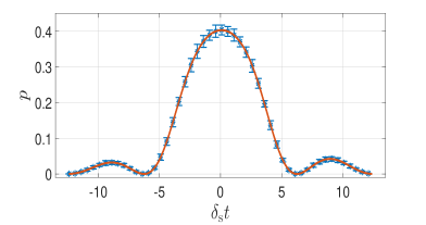
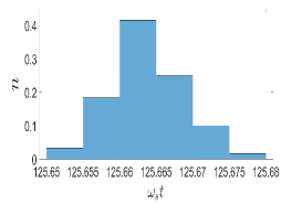
Refer to caption
Refer to caption
Refer to caption
Refer to caption
Figure 6: Preliminary estimation of the parameters achieved by varying δssubscript𝛿𝑠\delta_{s} and fitting the probability as a function of δs.subscript𝛿𝑠\delta_{s}. A numerical example is presented. The fit is shown in (a) and the estimation errors are presented in (b). While the ωssubscript𝜔s\omega_{\rm{s}} can be estimated efficiently , the estimation of ωrsubscript𝜔r\omega_{\rm{r}} is not good enough for resolution. For this illustration: σt=1,ωst=40πformulae-sequence𝜎𝑡1subscript𝜔s𝑡40𝜋\sigma t=1,\,\omega_{\rm{s}}t=40\pi and the number of measurements in each detuning is n=2104.𝑛2superscript104n=2\cdot 10^{4}.

The next step is to use the estimated ωs,σsubscript𝜔s𝜎\omega_{\rm{s}},\sigma to apply our method. One can treat ωs,σsubscript𝜔s𝜎\omega_{\rm{s}},\sigma as known and estimate ωr,subscript𝜔r\omega_{\rm{r}}, however this will create a bias (we also want to progressively improve the estimation of ωs,subscript𝜔s\omega_{\rm{s}}, such that the detuning of the pulses will be more accurate). Note that we cannot get information about three different parameters by measuring copies of the same density matrix (even if measuring different observables, the FI matrix will be singular). Therefore at least three different measurements are required: one measurement with δst=2π,subscript𝛿𝑠𝑡2𝜋\delta_{s}t=2\pi, the resonance condition for estimation of ωrsubscript𝜔r\omega_{\rm{r}} and two other measurements with the optimal detunings for estimating ωs,σ.subscript𝜔s𝜎\omega_{\rm{s}},\sigma. The FI about ωs,σsubscript𝜔s𝜎\omega_{\rm{s}},\sigma as a function of δssubscript𝛿𝑠\delta_{s} is shown in supplementary fig. 7. Quite interestingly for both ωs,σsubscript𝜔s𝜎\omega_{\rm{s}},\sigma the optimal δs2πtsubscript𝛿𝑠2𝜋𝑡\delta_{s}\rightarrow\frac{2\pi}{t} as σ𝜎\sigma\rightarrow\infty (this is because as σ𝜎\sigma becomes larger the exponential decay becomes stronger and one needs to get closer to δst=2πsubscript𝛿𝑠𝑡2𝜋\delta_{s}t=2\pi).

The optimal FI about ωssubscript𝜔s\omega_{\rm{s}} scales as σ2t4superscript𝜎2superscript𝑡4\sigma^{2}t^{4} and is comparable to the optimal FI about ωr.subscript𝜔r\omega_{\rm{r}}. The optimal FI about σ𝜎\sigma behaves in an unusual manner: Usually the FI about the amplitude grows as t2,superscript𝑡2t^{2}, while here the optimum (for σt>1𝜎𝑡1\sigma t>1) is Iσ0.63σ2.similar-tosubscript𝐼𝜎0.63superscript𝜎2I_{\sigma}\sim\frac{0.63}{\sigma^{2}}. It does not depend on t,𝑡t, and it drops as σ𝜎\sigma gets larger. This behavior is somewhat similar to sensing the standard deviation of the amplitude of a stationary signal (H=AσZ𝐻𝐴subscript𝜎𝑍H=A\sigma_{Z} where AN(0,σ)similar-to𝐴𝑁0𝜎A\sim N\left(0,\sigma\right)).

Since we are dealing with a multivariable estimation, the Cramér-Rao bound is given by the Fisher information matrix in the following way Cramér (2016): (Δx)2=(I1)x,x.superscriptΔ𝑥2subscriptsuperscript𝐼1𝑥𝑥\left(\Delta x\right)^{2}=\left(I^{-1}\right)_{x,x}. We would like then to calculate the FI matrix. The full expression of the matrix is quite involved, however we can easily observe that as ωr0subscript𝜔r0\omega_{\rm{r}}\rightarrow 0 the FI matrix converges to a block diagonal matrix, with Irsubscript𝐼rI_{\rm{r}} as one of its eigenvalues. The FI matrix per three measurements is the sum of the FI matrices of each measurement: I(1)+I(2)+I(3)superscript𝐼1superscript𝐼2superscript𝐼3I^{\left(1\right)}+I^{\left(2\right)}+I^{\left(3\right)}. Therefore the FI matrix per single measurement reads: I=13(I(1)+I(2)+I(3)).𝐼13superscript𝐼1superscript𝐼2superscript𝐼3I=\frac{1}{3}\left(I^{\left(1\right)}+I^{\left(2\right)}+I^{\left(3\right)}\right). Denoting the FI matrix that corresponds to δst=2πsubscript𝛿s𝑡2𝜋\delta_{\rm{s}}t=2\pi as I(1)superscript𝐼1I^{\left(1\right)}, we observe that:

(pωs)2p(1p),(pσ)2p(1p),(pσ)(pωr)p(1p),(pωs)(pωr)p(1p)0I(1)=(Ir00000000)superscript𝑝subscript𝜔s2𝑝1𝑝superscript𝑝𝜎2𝑝1𝑝𝑝𝜎𝑝subscript𝜔r𝑝1𝑝𝑝subscript𝜔s𝑝subscript𝜔r𝑝1𝑝0superscript𝐼1subscript𝐼r00000000\frac{\left(\frac{\partial p}{\partial\omega_{{\rm s}}}\right)^{2}}{p\left(1-p\right)},\frac{\left(\frac{\partial p}{\partial\sigma}\right)^{2}}{p\left(1-p\right)},\frac{\left(\frac{\partial p}{\partial\sigma}\right)\left(\frac{\partial p}{\partial\omega_{{\rm r}}}\right)}{p\left(1-p\right)},\frac{\left(\frac{\partial p}{\partial\omega_{{\rm s}}}\right)\left(\frac{\partial p}{\partial\omega_{{\rm r}}}\right)}{p\left(1-p\right)}\rightarrow 0\Longrightarrow I^{\left(1\right)}=\left(\begin{array}[]{ccc}I_{{\rm r}}&0&0\\ 0&0&0\\ 0&0&0\end{array}\right) (67)

Regarding I(2),I(3)superscript𝐼2superscript𝐼3I^{\left(2\right)},I^{\left(3\right)}, note that for them (since δst2πnsubscript𝛿𝑠𝑡2𝜋𝑛\delta_{s}t\neq 2\pi n) we have that:

(pωr)2p(1p),(pωr)(pωs)p(1p),(pωr)(pσ)p(1p)0I(j)=(0000I2,2(j)I2,3(j)0I3,2(j)I3,3(j)).superscript𝑝subscript𝜔r2𝑝1𝑝𝑝subscript𝜔r𝑝subscript𝜔s𝑝1𝑝𝑝subscript𝜔r𝑝𝜎𝑝1𝑝0superscript𝐼𝑗0000superscriptsubscript𝐼22𝑗superscriptsubscript𝐼23𝑗0superscriptsubscript𝐼32𝑗superscriptsubscript𝐼33𝑗\frac{\left(\frac{\partial p}{\partial\omega_{{\rm r}}}\right)^{2}}{p\left(1-p\right)},\frac{\left(\frac{\partial p}{\partial\omega_{{\rm r}}}\right)\left(\frac{\partial p}{\partial\omega_{{\rm s}}}\right)}{p\left(1-p\right)},\frac{\left(\frac{\partial p}{\partial\omega_{{\rm r}}}\right)\left(\frac{\partial p}{\partial\sigma}\right)}{p\left(1-p\right)}\rightarrow 0\Longrightarrow I^{\left(j\right)}=\left(\begin{array}[]{ccc}0&0&0\\ 0&I_{2,2}^{\left(j\right)}&I_{2,3}^{\left(j\right)}\\ 0&I_{3,2}^{\left(j\right)}&I_{3,3}^{\left(j\right)}\end{array}\right). (68)

Therefore the FI matrix per single measurement reads:

I=13(Ir000I2,2I2,30I3,2I3,3),𝐼13subscript𝐼r000subscript𝐼22subscript𝐼230subscript𝐼32subscript𝐼33I=\frac{1}{3}\left(\begin{array}[]{ccc}I_{{\rm r}}&0&0\\ 0&I_{2,2}&I_{2,3}\\ 0&I_{3,2}&I_{3,3}\end{array}\right), (69)

and thus Δωr=3IrΔsubscript𝜔r3subscript𝐼𝑟\Delta\omega_{\rm{r}}=\sqrt{\frac{3}{I_{r}}}, we therefore get an extra factor of 33\sqrt{3} due to these chunks of three measurements. The standard deviation obtained in practice (with MLE) is a bit above the expected analytical values, as can be seen in supplementary fig. 8.
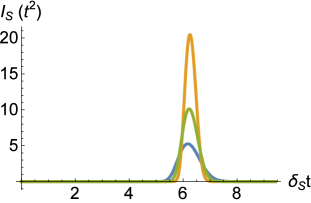
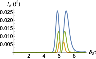
Refer to caption
Refer to caption
Figure 7: (a) The FI about ωssubscript𝜔s\omega_{\rm{s}} as function of δstsubscript𝛿𝑠𝑡\delta_{s}t for different values of σ𝜎\sigma (σt=5𝜎𝑡5\sigma t=5:  Orange, σt=7𝜎𝑡7\sigma t=7:  Green, σt=10𝜎𝑡10\sigma t=10:  Blue ).
(b) The FI about σ𝜎\sigma as function of δstsubscript𝛿𝑠𝑡\delta_{s}t for different values of σ𝜎\sigma (same colors). In both plots ωr=0.subscript𝜔r0\omega_{\rm{r}}=0. Interestingly, as σt𝜎𝑡\sigma t\rightarrow\infty the optimal δst2π.subscript𝛿𝑠𝑡2𝜋\delta_{s}t\rightarrow 2\pi.
Refer to caption
Refer to caption
Refer to caption
Refer to caption
Refer to caption
Figure 8: The second stage of the protocol consists of measurements in three different detunings (each one is optimal for the estimation of a different parameter; one of them is therefore δs=2πtsubscript𝛿𝑠2𝜋𝑡\delta_{s}=\frac{2\pi}{t}). In this example: δst=0.01,subscript𝛿𝑠𝑡0.01\delta_{s}t=0.01, σt=5𝜎𝑡5\sigma t=5 and the number of measurements in each detuning is N=3105.𝑁3superscript105N=3\cdot 10^{5}. The histograms for the different parameters are presented in (a). It can be seen that resolution is achieved as Δωr=17.5ωr.Δsubscript𝜔r17.5subscript𝜔r\Delta\omega_{\rm{r}}=\frac{1}{7.5}\omega_{\rm{r}}. In (b) the histograms of ω1,ω2subscript𝜔1subscript𝜔2\omega_{1},\omega_{2} are presented, it can be seen that the frequencies are clearly resolved. (c) The RMSE (root mean square error) in estimating the parameters as a function of N.𝑁N. The solid lines are the theoretical expectations (green (bottom): Δωs,Δsubscript𝜔s\Delta\omega_{\rm{s}}, orange (middle): Δωr,Δsubscript𝜔r\Delta\omega_{\rm{r}}, blue (top): ΔσΔ𝜎\Delta\sigma). The points represent the RMSE achieved in an actual maximum likelihood estimation (green (diamonds):Δωs,Δsubscript𝜔s\Delta\omega_{\rm{s}}, orange (circles): Δωr,Δsubscript𝜔r\Delta\omega_{\rm{r}}, blue (squares): ΔσΔ𝜎\Delta\sigma). It can be seen that there is no divergence: The RMSE of all the parameters scale as N0.5.superscript𝑁0.5N^{-0.5}. In fact ΔωrΔsubscript𝜔r\Delta\omega_{\rm{r}} is very close to Δωs,Δsubscript𝜔s\Delta\omega_{\rm{s}}, whereas the worst is ΔσΔ𝜎\Delta\sigma.

Appendix H Limitation due to incoherence

In this part we derive the effect of incoherence of the signal (during the measurement) on the method, where we consider a model in which the quadratures undergo identical and independent OU process. The OU process is defined as dAi=γAidt+σndWtAi,𝑑subscript𝐴𝑖𝛾subscript𝐴𝑖𝑑𝑡subscript𝜎𝑛𝑑superscriptsubscript𝑊𝑡subscript𝐴𝑖dA_{i}=-\gamma A_{i}\,dt+\sigma_{n}\,dW_{t}^{A_{i}}, and similarly for Bi.subscript𝐵𝑖B_{i}. To get the effect, we need to calculate the transition probability p=sin(ϕ)2,p=\langle\sin\left(\phi\right)^{2}\rangle, where ϕitalic-ϕ\phi is the accumulated phase. Note that:

ϕ=i=120𝑇(Ai(t)cos(ωit)+Bi(t)sin(ωit))dt,italic-ϕ2𝑖1𝑇0subscript𝐴𝑖𝑡subscript𝜔𝑖𝑡subscript𝐵𝑖𝑡subscript𝜔𝑖𝑡𝑑𝑡\phi=\overset{2}{\underset{i=1}{\sum}}\overset{T}{\underset{0}{\int}}\left(A_{i}\left(t\right)\cos\left(\omega_{i}t\right)+B_{i}\left(t\right)\sin\left(\omega_{i}t\right)\right)\>dt, (70)

where Ai(t)=Ai(0)exp(γt)+σn0𝑡eγ(ts)dWsAi,subscript𝐴𝑖𝑡subscript𝐴𝑖0𝛾𝑡subscript𝜎𝑛𝑡0superscript𝑒𝛾𝑡𝑠𝑑superscriptsubscript𝑊𝑠subscript𝐴𝑖A_{i}\left(t\right)=A_{i}\left(0\right)\exp\left(-\gamma t\right)+\sigma_{n}\overset{t}{\underset{0}{\int}}e^{-\gamma\left(t-s\right)}dW_{s}^{A_{i}}, and the same holds for Bi(t).subscript𝐵𝑖𝑡B_{i}\left(t\right). Therefore ϕitalic-ϕ\phi can be written as the sum ϕ=ϕav+ϕn,italic-ϕsubscriptitalic-ϕ𝑎𝑣subscriptitalic-ϕ𝑛\phi=\phi_{av}+\phi_{n}, where:

ϕav=i=120𝑇(Ai(0)eγtcos(ωit)+Bi(0)eγtsin(ωit))dt,subscriptitalic-ϕ𝑎𝑣2𝑖1𝑇0subscript𝐴𝑖0superscript𝑒𝛾𝑡subscript𝜔𝑖𝑡subscript𝐵𝑖0superscript𝑒𝛾𝑡subscript𝜔𝑖𝑡𝑑𝑡\phi_{av}=\overset{2}{\underset{i=1}{\sum}}\overset{T}{\underset{0}{\int}}\left(A_{i}\left(0\right)e^{-\gamma t}\cos\left(\omega_{i}t\right)+B_{i}\left(0\right)e^{-\gamma t}\sin\left(\omega_{i}t\right)\right)\>dt, (71)

and:

ϕn=i=12σn0𝑇dt(cos(ωit)0𝑡eγ(ts)dWsAi+sin(ωit)0𝑡eγ(ts)dWsBi).subscriptitalic-ϕ𝑛2𝑖1subscript𝜎𝑛𝑇0𝑑𝑡subscript𝜔𝑖𝑡0𝑡superscript𝑒𝛾𝑡𝑠𝑑superscriptsubscript𝑊𝑠subscript𝐴𝑖subscript𝜔𝑖𝑡0𝑡superscript𝑒𝛾𝑡𝑠𝑑superscriptsubscript𝑊𝑠subscript𝐵𝑖\phi_{n}=\overset{2}{\underset{i=1}{\sum}}\sigma_{n}\overset{T}{\underset{0}{\int}}dt\>\left(\cos\left(\omega_{i}t\right)\underset{0}{\overset{t}{\int}}e^{-\gamma\left(t-s\right)}dW_{s}^{A_{i}}+\sin\left(\omega_{i}t\right)\underset{0}{\overset{t}{\int}}e^{-\gamma\left(t-s\right)}dW_{s}^{B_{i}}\right). (72)

Observe that ϕnsubscriptitalic-ϕ𝑛\phi_{n} is a Gaussian random variable with ϕn=0,delimited-⟨⟩subscriptitalic-ϕ𝑛0\langle\phi_{n}\rangle=0, and:

ϕn2=i=12σn20𝑇ds[𝑠𝑇cos(ωit)eγ(ts)dt]2+𝑖σn20𝑇ds[𝑠𝑇sin(ωit)eγ(ts)dt]2delimited-⟨⟩superscriptsubscriptitalic-ϕ𝑛22𝑖1superscriptsubscript𝜎𝑛2𝑇0𝑑𝑠superscriptdelimited-[]𝑠𝑇subscript𝜔𝑖𝑡superscript𝑒𝛾𝑡𝑠𝑑𝑡2𝑖superscriptsubscript𝜎𝑛2𝑇0𝑑𝑠superscriptdelimited-[]𝑠𝑇subscript𝜔𝑖𝑡superscript𝑒𝛾𝑡𝑠𝑑𝑡2\langle\phi_{n}^{2}\rangle=\overset{2}{\underset{i=1}{\sum}}\sigma_{n}^{2}\overset{T}{\underset{0}{\int}}ds\left[\underset{s}{\overset{T}{\int}}\cos\left(\omega_{i}t\right)e^{-\gamma\left(t-s\right)}\>dt\right]^{2}+\underset{i}{\sum}\sigma_{n}^{2}\overset{T}{\underset{0}{\int}}ds\left[\underset{s}{\overset{T}{\int}}\sin\left(\omega_{i}t\right)e^{-\gamma\left(t-s\right)}\>dt\right]^{2} (73)

We would like now to take ωsT=2πsubscript𝜔s𝑇2𝜋\omega_{\rm{s}}T=2\pi in the regime of: γT1,ϕn1,ωrT1.formulae-sequencemuch-less-than𝛾𝑇1formulae-sequencemuch-less-thansubscriptitalic-ϕ𝑛1much-less-thansubscript𝜔r𝑇1\gamma T\ll 1,\>\phi_{n}\ll 1,\>\omega_{\rm{r}}T\ll 1. In this case p=sin(ϕ)2ϕav2+ϕn2.p=\langle\sin\left(\phi\right)^{2}\rangle\approx\langle\phi_{av}^{2}\rangle+\langle\phi_{n}^{2}\rangle. In leading orders:

ϕn2σn2T3(1π2+O(γT)),delimited-⟨⟩superscriptsubscriptitalic-ϕ𝑛2superscriptsubscript𝜎𝑛2superscript𝑇31superscript𝜋2𝑂𝛾𝑇\langle\phi_{n}^{2}\rangle\approx\sigma_{n}^{2}T^{3}\left(\frac{1}{\pi^{2}}+O\left(\gamma T\right)\right), (74)

and:

ϕav2[(A1(0)A2(0))2πωrT2+i=12Bi(0)γT22π]2==i=12Ai(0)214π2ωr2T4+i=12Bi(0)214π2γ2T4==σn24π2γωr2T4+σn24π2γT4.delimited-⟨⟩superscriptsubscriptitalic-ϕ𝑎𝑣2delimited-⟨⟩superscriptdelimited-[]subscript𝐴10subscript𝐴202𝜋subscript𝜔rsuperscript𝑇22𝑖1subscript𝐵𝑖0𝛾superscript𝑇22𝜋22𝑖1delimited-⟨⟩subscript𝐴𝑖superscript0214superscript𝜋2superscriptsubscript𝜔r2superscript𝑇42𝑖1delimited-⟨⟩subscript𝐵𝑖superscript0214superscript𝜋2superscript𝛾2superscript𝑇4superscriptsubscript𝜎𝑛24superscript𝜋2𝛾superscriptsubscript𝜔r2superscript𝑇4superscriptsubscript𝜎𝑛24superscript𝜋2𝛾superscript𝑇4\displaystyle\begin{split}&\langle\phi_{av}^{2}\rangle\approx\langle\left[\frac{\left(A_{1}\left(0\right)-A_{2}\left(0\right)\right)}{2\pi}\omega_{\rm{r}}T^{2}+\overset{2}{\underset{i=1}{\sum}}B_{i}\left(0\right)\frac{\gamma T^{2}}{2\pi}\right]^{2}\rangle=\\ &=\overset{2}{\underset{i=1}{\sum}}\langle A_{i}\left(0\right)^{2}\rangle\frac{1}{4\pi^{2}}\omega_{\rm{r}}^{2}T^{4}+\overset{2}{\underset{i=1}{\sum}}\langle B_{i}\left(0\right)^{2}\rangle\frac{1}{4\pi^{2}}\gamma^{2}T^{4}=\\ &=\frac{\sigma_{n}^{2}}{4\pi^{2}\gamma}\omega_{\rm{r}}^{2}T^{4}+\frac{\sigma_{n}^{2}}{4\pi^{2}}\gamma T^{4}.\end{split} (75)

The second term (𝑖σn24π2γT4𝑖superscriptsubscript𝜎𝑛24superscript𝜋2𝛾superscript𝑇4\underset{i}{\sum}\frac{\sigma_{n}^{2}}{4\pi^{2}}\gamma T^{4}) can be neglected as it is much smaller than ϕn2σn2T3.similar-todelimited-⟨⟩superscriptsubscriptitalic-ϕ𝑛2superscriptsubscript𝜎𝑛2superscript𝑇3\langle\phi_{n}^{2}\rangle\sim\sigma_{n}^{2}T^{3}. Therefore:

pϕav2+ϕn2σn2T3π2+σn24π2γωr2T4,𝑝delimited-⟨⟩superscriptsubscriptitalic-ϕ𝑎𝑣2delimited-⟨⟩superscriptsubscriptitalic-ϕ𝑛2superscriptsubscript𝜎𝑛2superscript𝑇3superscript𝜋2superscriptsubscript𝜎𝑛24superscript𝜋2𝛾superscriptsubscript𝜔r2superscript𝑇4p\approx\langle\phi_{av}^{2}\rangle+\langle\phi_{n}^{2}\rangle\approx\frac{\sigma_{n}^{2}T^{3}}{\pi^{2}}+\frac{\sigma_{n}^{2}}{4\pi^{2}\gamma}\omega_{\rm{r}}^{2}T^{4}, (76)

using the notation in the main text σn2T3π2=nsuperscriptsubscript𝜎𝑛2superscript𝑇3superscript𝜋2𝑛\frac{\sigma_{n}^{2}T^{3}}{\pi^{2}}=n, and the resolution condition is thus ωr2Tγ1.much-greater-thansuperscriptsubscript𝜔r2𝑇𝛾1\omega_{\rm{r}}^{2}\frac{T}{\gamma}\gg 1.

Appendix I Limitation due to dephasing of the probe

Let us now find the implications of noise inflicted on the probe: specifically we consider a Markovian dephasing. Intuitively this should set an additional limitation: the transition probability does not vanish now due to two reasons: the finite ωr,subscript𝜔r\omega_{\rm{r}}, namely the term (σt)2(ωrt)2,superscript𝜎𝑡2superscriptsubscript𝜔r𝑡2\left(\sigma t\right)^{2}\left(\omega_{\rm{r}}t\right)^{2}, and also due to a dephasing rate of κ,𝜅\kappa, namely a term of κt.𝜅𝑡\kappa t. Hence resolution can be achieved if the first term is larger than the second, hence the condition is ωrσ(κ2)1.much-greater-thansubscript𝜔r𝜎superscript𝜅21\frac{\omega_{\rm{r}}\sigma}{\left(\kappa^{2}\right)}\gg 1.

In more detail, given our Hamiltonian H=f(t)σz𝐻𝑓𝑡subscript𝜎𝑧H=f\left(t\right)\sigma_{z} and a dephasing rate κ,𝜅\kappa, the time evolution is given by the Master equation:

dρdt=i[f(t)σz,ρ]+κ(σzρσzρ).𝑑𝜌𝑑𝑡𝑖𝑓𝑡subscript𝜎𝑧𝜌𝜅subscript𝜎𝑧𝜌subscript𝜎𝑧𝜌\frac{d\rho}{dt}=-i\left[f\left(t\right)\sigma_{z},\rho\right]+\kappa\left(\sigma_{z}\rho\sigma_{z}-\rho\right). (77)

Initializing and measuring in σxsubscript𝜎𝑥\sigma_{x} basis, we get the transition probability p=0.50.5e2κtcos(2ϕ)𝑝0.50.5superscript𝑒2𝜅𝑡2italic-ϕp=0.5-0.5e^{-2\kappa t}\cos\left(2\phi\right) (where ϕitalic-ϕ\phi is the accumulated phase). Averaging over the different realizations we get: p=0.5(1exp((σt)2(ωrt)2π22κt)),𝑝0.51superscript𝜎𝑡2superscriptsubscript𝜔r𝑡2superscript𝜋22𝜅𝑡p=0.5\left(1-\exp\left(-\frac{\left(\sigma t\right)^{2}\left(\omega_{\rm{r}}t\right)^{2}}{\pi^{2}}-2\kappa t\right)\right), and the FI reads:

Ir=4ωr2σ4t8π4[(exp(4κt+2ωr2σ2t4/π2)1)].subscript𝐼r4superscriptsubscript𝜔r2superscript𝜎4superscript𝑡8superscript𝜋4delimited-[]4𝜅𝑡2superscriptsubscript𝜔r2superscript𝜎2superscript𝑡4superscript𝜋21I_{\rm{r}}=\frac{4\omega_{\rm{r}}^{2}\sigma^{4}t^{8}}{\pi^{4}\left[\left(\exp\left(4\kappa t+2\omega_{\rm{r}}^{2}\sigma^{2}t^{4}/\pi^{2}\right)-1\right)\right]}. (78)

Hence the noiseless FI is retrieved only for ωrσ(κ2)1.much-greater-thansubscript𝜔r𝜎superscript𝜅21\frac{\omega_{\rm{r}}\sigma}{\left(\kappa^{2}\right)}\gg 1. Note that the effect of dephasing in this problem is quite different: first, the FI is not necessarily close to the noiseless FI for κt1,much-less-than𝜅𝑡1\kappa t\ll 1, the condition ωrσ(κ2)1much-greater-thansubscript𝜔r𝜎superscript𝜅21\frac{\omega_{\rm{r}}\sigma}{\left(\kappa^{2}\right)}\gg 1 must hold. Second, since there is a competition between (σt)2(ωrt)2superscript𝜎𝑡2superscriptsubscript𝜔r𝑡2\left(\sigma t\right)^{2}\left(\omega_{\rm{r}}t\right)^{2} and κt,𝜅𝑡\kappa t, and for short enough times the second term is always larger, then the noiseless FI is retrieved only after a minimal time (goes as κ1/3σ2/3ωr2/3similar-toabsentsuperscript𝜅13superscript𝜎23superscriptsubscript𝜔r23\sim\frac{\kappa^{1/3}}{\sigma^{2/3}\omega_{\rm{r}}^{2/3}}) . This behavior is illustrated in supplementary fig. 9.
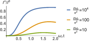
Refer to caption
Figure 9: The FI with dephasing (Insuperscript𝐼𝑛I^{n}) divided by the noiseless FI (I0superscript𝐼0I^{0}), for different values of σωrκ2.𝜎subscript𝜔rsuperscript𝜅2\frac{\sigma\omega_{\rm{r}}}{\kappa^{2}}. Note that as σωrκ2𝜎subscript𝜔rsuperscript𝜅2\frac{\sigma\omega_{\rm{r}}}{\kappa^{2}} gets higher the noisy FI can get closer to the noiseless FI, however there is a minimal time from which this can be achieved. This minimal time goes as κ1/3σ2/3ωr2/3similar-toabsentsuperscript𝜅13superscript𝜎23superscriptsubscript𝜔r23\sim\frac{\kappa^{1/3}}{\sigma^{2/3}\omega_{\rm{r}}^{2/3}}.

We therefore observe that Markovian noise on the qubit (such as dephasing) imposes a resolution limit, this invokes a natural question: can error correction protocols remove these limitations imposed by Markovian noise? Note that this question is not analogous to the achievability of Heisenberg scaling which was addressed in Sekatski et al. (2017); Zhou et al. (2018); Demkowicz-Dobrzański et al. (2017). The prospects for quantum error correction in these resolution problems are left for future work, however we point out that this limit can be eliminated provided that errors can be detected, since one does not need to correct the errors. Given that error detection is possible, we can postselect the measurements without error and perform estimation according to them. These errors thus reduce the precision, but they do not impose a limitation. This implies that the error correction condition to remove limitation in this problem should be different from the error correction condition for Heisenberg scaling. Let us denote the jump operators in the Master equation as {Lj}j.subscriptsubscript𝐿𝑗𝑗\left\{L_{j}\right\}_{j}. For Heisenberg scaling, the error correction condition is Hspan{I,Lj,Lj,LiLj}i,,jH\notin\text{span}\left\{I,L_{j},L_{j}^{\dagger},L_{i}^{\dagger}L_{j}\right\}_{i,,j} Sekatski et al. (2017); Zhou et al. (2018); Demkowicz-Dobrzański et al. (2017), since we need both to detect and to correct. In this case, since we need only to detect, the error correction condition should be: Hspan{I,Lj,Lj}j.𝐻spansubscript𝐼superscriptsubscript𝐿𝑗subscript𝐿𝑗𝑗H\notin\text{span}\left\{I,L_{j}^{\dagger},L_{j}\right\}_{j}. This implies, for example, that if the only noise source is amplitude damping (namely the only jump operator is σsubscript𝜎\sigma_{-}), then detection is possible, and we can overcome the limitation.

Appendix J Superresolution with QFT

Consider the Hamiltonian in supplementary eq. 48, and assume a relatively long coherence time (in which phases and amplitudes are constant), such that sampling is performed. Namely Ramsey measurements are performed in different times, as it is described in Schmitt et al. (2017); Boss et al. (2017); Glenn et al. (2018). The length of each measurement is τ𝜏\tau and the total sampling time is T=Nτ.𝑇𝑁𝜏T=N\tau. The standard way to analyze this data is to perform a Fourier transform and fit the power spectrum. However this method suffers from a resolution limit Rotem et al. (2019), since the probability is symmetric with respect to ωrsubscript𝜔r\omega_{\rm{r}} and the noise does not vanish.

We claim that storing the data in a quantum state (using memory qubits) and using the same trick of nullifying the projection noise, then resolution limit can be beaten. In a standard Ramsey experiment the state of the probe, after phase accumulation, is 12(|0+eiϕ|1).12ket0superscript𝑒𝑖italic-ϕket1\frac{1}{\sqrt{2}}\left(|0\rangle+e^{i\phi}|1\rangle\right). If we entangle the probe to memory qubits in each phase acquisition, the following state of the memory qubits can be generated:

|ψ=1N(j=0N1|jeiϕj),ket𝜓1𝑁𝑗0𝑁1ket𝑗superscript𝑒𝑖subscriptitalic-ϕ𝑗|\psi\rangle=\frac{1}{\sqrt{N}}\left(\underset{j=0}{\overset{N-1}{\sum}}|j\rangle e^{i\phi_{j}}\right), (79)

where ϕj=τ[𝑖Aicos(ωitj)+Bisin(ωitj)],(tj=jτ).subscriptitalic-ϕ𝑗𝜏delimited-[]𝑖subscript𝐴𝑖subscript𝜔𝑖subscript𝑡𝑗subscript𝐵𝑖subscript𝜔𝑖subscript𝑡𝑗subscript𝑡𝑗𝑗𝜏\phi_{j}=\tau\left[\underset{i}{\sum}A_{i}\cos\left(\omega_{i}t_{j}\right)+B_{i}\sin\left(\omega_{i}t_{j}\right)\right],\;(t_{j}=j\tau). The idea is that for ωr=0subscript𝜔r0\omega_{\rm{r}}=0 only harmonics of ωssubscript𝜔s\omega_{\rm{s}} can be measured, and the probability to measure the other frequencies goes as ωr2.superscriptsubscript𝜔r2\omega_{\rm{r}}^{2}. To see this note that

ϕj(ωr=0)=τ[𝑖Aicos(ωstj)+Bisin(ωstj)]=Ωsin(ωstj+φ),subscriptitalic-ϕ𝑗subscript𝜔r0𝜏delimited-[]𝑖subscript𝐴𝑖subscript𝜔ssubscript𝑡𝑗subscript𝐵𝑖subscript𝜔ssubscript𝑡𝑗Ωsubscript𝜔ssubscript𝑡𝑗𝜑\phi_{j}\left(\omega_{\rm{r}}=0\right)=\tau\left[\underset{i}{\sum}A_{i}\cos\left(\omega_{\rm{s}}t_{j}\right)+B_{i}\sin\left(\omega_{\rm{s}}t_{j}\right)\right]=\Omega\sin\left(\omega_{\rm{s}}t_{j}+\varphi\right), (80)

and therefore:

eiϕj(ωr=0)=k=Jk(Ω)exp(ikφ)exp(ikωsjτ),superscript𝑒𝑖subscriptitalic-ϕ𝑗subscript𝜔r0𝑘infinitysubscript𝐽𝑘Ω𝑖𝑘𝜑𝑖𝑘subscript𝜔s𝑗𝜏e^{i\phi_{j}\left(\omega_{\rm{r}}=0\right)}=\underset{k=-\infty}{\overset{\infty}{\sum}}J_{k}\left(\Omega\right)\exp\left(ik\varphi\right)\exp\left(ik\omega_{\rm{s}}j\tau\right), (81)

where this expansion to harmonics of ωssubscript𝜔s\omega_{\rm{s}} is the Jacobi-Anger expansion.

Since we want to make sure that ωssubscript𝜔s\omega_{\rm{s}} (and integer multiples of it) will be included in the Fourier basis, we need to set T=2πωsm𝑇2𝜋subscript𝜔s𝑚T=\frac{2\pi}{\omega_{\rm{s}}}m (integer m𝑚m). In order to avoid too many harmonics, we also set τ=2πωs1n𝜏2𝜋subscript𝜔s1𝑛\tau=\frac{2\pi}{\omega_{\rm{s}}}\frac{1}{n} (integer n𝑛n).

It is now simple to see that with this choice, the only frequencies that can be measured in QFT are: 0,ωs,,(n1)ωs,0subscript𝜔s𝑛1subscript𝜔s0,\omega_{\rm{s}},...,\left(n-1\right)\omega_{\rm{s}}, as the state reads:

|ψ0=l=0n1al|lωs,ketsubscript𝜓0𝑙0𝑛1subscript𝑎𝑙ket𝑙subscript𝜔s|\psi_{0}\rangle=\underset{l=0}{\overset{n-1}{\sum}}a_{l}|l\omega_{\rm{s}}\rangle, (82)

where al=k=Jnk+l(Ω)exp(i(nk+l)φ).subscript𝑎𝑙𝑘infinitysubscript𝐽𝑛𝑘𝑙Ω𝑖𝑛𝑘𝑙𝜑a_{l}=\underset{k=-\infty}{\overset{\infty}{\sum}}J_{nk+l}\left(\Omega\right)\exp\left(i\left(nk+l\right)\varphi\right).

So for example given a noise model of a random phase, the density matrix is diagonal in the Fourier basis: ρ=l=0n1pl|lωslωs|,𝜌𝑙0𝑛1subscript𝑝𝑙ket𝑙subscript𝜔sbra𝑙subscript𝜔s\rho=\underset{l=0}{\overset{n-1}{\sum}}p_{l}|l\omega_{\rm{s}}\rangle\langle l\omega_{\rm{s}}|, where pl=k=|Jnk+l(Ω)|2,subscript𝑝𝑙𝑘infinitysuperscriptsubscript𝐽𝑛𝑘𝑙Ω2p_{l}=\underset{k=-\infty}{\overset{\infty}{\sum}}|J_{nk+l}\left(\Omega\right)|^{2}, hence the optimal measurement basis is the Fourier basis (and it is enough to measure whether we get harmonics of ωssubscript𝜔s\omega_{\rm{s}} or not).

Refer to caption
Figure 10: Illustration of superresolution with QFT: probabilities of the different frequencies for ωr=0subscript𝜔r0\omega_{\rm{r}}=0 (dashed, orange lines) and ωrT=0.05subscript𝜔r𝑇0.05\omega_{\rm{r}}T=0.05 (solid, blue line). The probabilities to measure frequencies that are not harmonics of ωssubscript𝜔s\omega_{\rm{s}} goes as ωr2,superscriptsubscript𝜔r2\omega_{\rm{r}}^{2}, and thus superresolution can be achieved by measuring these frequencies. In this illustration, the quadratures are random with στ=1,𝜎𝜏1\sigma\tau=1, and the number of repetitions is 105.superscript10510^{5}.

Let us now find the probability to measure frequencies that are not harmonics of ωssubscript𝜔s\omega_{\rm{s}}, for ωrT1.much-less-thansubscript𝜔r𝑇1\omega_{\rm{r}}T\ll 1. We denote the projector on the other frequencies (not harmonics of ωssubscript𝜔s\omega_{\rm{s}}) as Π,Π\Pi, so we are interested in finding p=|Π|ψ|2.𝑝superscriptΠket𝜓2p=|\Pi|\psi\rangle|^{2}. Of course: |ψ=|ψ0+ωrd|ψdωr+𝒪(ωr2),ket𝜓ketsubscript𝜓0subscript𝜔r𝑑ket𝜓𝑑subscript𝜔r𝒪superscriptsubscript𝜔r2|\psi\rangle=|\psi_{0}\rangle+\omega_{\rm{r}}\frac{d|\psi\rangle}{d\omega_{\rm{r}}}+\mathcal{O}\left(\omega_{\rm{r}}^{2}\right), and since Π|ψ0=0,Πketsubscript𝜓00\Pi|\psi_{0}\rangle=0, we get that: pωr2|Πd|ψdωr|2.𝑝superscriptsubscript𝜔r2superscriptΠ𝑑ket𝜓𝑑subscript𝜔r2p\approx\omega_{\rm{r}}^{2}|\Pi\frac{d|\psi\rangle}{d\omega_{\rm{r}}}|^{2}. Now:

d|ψdωr=j=1𝑁exp(iϕj(ωr=0))(iωrtj)[(B1B2)τcos(ωstj)+(A2A1)τsin(ωstj)]|j,𝑑ket𝜓𝑑subscript𝜔r𝑗1𝑁𝑖subscriptitalic-ϕ𝑗subscript𝜔r0𝑖subscript𝜔rsubscript𝑡𝑗delimited-[]subscript𝐵1subscript𝐵2𝜏subscript𝜔ssubscript𝑡𝑗subscript𝐴2subscript𝐴1𝜏subscript𝜔ssubscript𝑡𝑗ket𝑗\frac{d|\psi\rangle}{d\omega_{\rm{r}}}=\underset{j=1}{\overset{N}{\sum}}\exp\left(i\phi_{j}\left(\omega_{\rm{r}}=0\right)\right)\left(i\omega_{\rm{r}}t_{j}\right)\left[\left(B_{1}-B_{2}\right)\tau\cos\left(\omega_{\rm{s}}t_{j}\right)+\left(A_{2}-A_{1}\right)\tau\sin\left(\omega_{\rm{s}}t_{j}\right)\right]|j\rangle,

note that we can expand:

exp(iϕj(ωr=0))[(B1B2)τcos(ωstj)+(A2A1)τsin(ωstj)]=l=0n1blexp(ilωstj),𝑖subscriptitalic-ϕ𝑗subscript𝜔r0delimited-[]subscript𝐵1subscript𝐵2𝜏subscript𝜔ssubscript𝑡𝑗subscript𝐴2subscript𝐴1𝜏subscript𝜔ssubscript𝑡𝑗𝑙0𝑛1subscript𝑏𝑙𝑖𝑙subscript𝜔ssubscript𝑡𝑗\exp\left(i\phi_{j}\left(\omega_{\rm{r}}=0\right)\right)\left[\left(B_{1}-B_{2}\right)\tau\cos\left(\omega_{\rm{s}}t_{j}\right)+\left(A_{2}-A_{1}\right)\tau\sin\left(\omega_{\rm{s}}t_{j}\right)\right]=\underset{l=0}{\overset{n-1}{\sum}}b_{l}\exp\left(il\omega_{\rm{s}}t_{j}\right), (83)

Therefore:

d|ψdωr=iNl=0n1blj=0N1tjexp(ilωstj)|j.𝑑ket𝜓𝑑subscript𝜔r𝑖𝑁𝑙0𝑛1subscript𝑏𝑙𝑗0𝑁1subscript𝑡𝑗𝑖𝑙subscript𝜔ssubscript𝑡𝑗ket𝑗\frac{d|\psi\rangle}{d\omega_{\rm{r}}}=\frac{i}{\sqrt{N}}\underset{l=0}{\overset{n-1}{\sum}}b_{l}\underset{j=0}{\overset{N-1}{\sum}}t_{j}\exp\left(il\omega_{\rm{s}}t_{j}\right)|j\rangle. (84)

For convenience let us denote |rk=1Nj=1𝑁tjexp(ikωstj)|j,ketsubscript𝑟𝑘1𝑁𝑗1𝑁subscript𝑡𝑗𝑖𝑘subscript𝜔ssubscript𝑡𝑗ket𝑗|r_{k}\rangle=\frac{1}{\sqrt{N}}\underset{j=1}{\overset{N}{\sum}}t_{j}\exp\left(ik\omega_{\rm{s}}t_{j}\right)|j\rangle, then with this notation:

d|ψdωr=il=0n1bl|rl.𝑑ket𝜓𝑑subscript𝜔r𝑖𝑙0𝑛1subscript𝑏𝑙ketsubscript𝑟𝑙\frac{d|\psi\rangle}{d\omega_{\rm{r}}}=i\underset{l=0}{\overset{n-1}{\sum}}b_{l}|r_{l}\rangle. (85)

Now given that T2πωs,much-greater-than𝑇2𝜋subscript𝜔sT\gg\frac{2\pi}{\omega_{\rm{s}}}, the state |rlketsubscript𝑟𝑙|r_{l}\rangle will have a non-negligible overlap only with frequencies close enough to |lωs,ket𝑙subscript𝜔s|l\omega_{\rm{s}}\rangle, this leads us to make two approximations: ikrk|Π|ri=0𝑖𝑘quantum-operator-productsubscript𝑟𝑘Πsubscript𝑟𝑖0i\neq k\Rightarrow\langle r_{k}|\Pi|r_{i}\rangle=0 (different |rkketsubscript𝑟𝑘|r_{k}\rangle’s overlap orthogonal frequencies) and |Π|rk|2=rk|rk|kωs|rk|2superscriptΠketsubscript𝑟𝑘2inner-productsubscript𝑟𝑘subscript𝑟𝑘superscriptinner-product𝑘subscript𝜔ssubscript𝑟𝑘2|\Pi|r_{k}\rangle|^{2}=\langle r_{k}|r_{k}\rangle-|\langle k\omega_{\rm{s}}|r_{k}\rangle|^{2} (the only harmonic that overlaps |rkketsubscript𝑟𝑘|r_{k}\rangle is |kωsket𝑘subscript𝜔s|k\omega_{\rm{s}}\rangle).

Due to the first approximation:

pωr2|Πd|ψdωr|2ωr2l=0n1|bl|2|Π|rl|2.𝑝superscriptsubscript𝜔r2superscriptΠ𝑑ket𝜓𝑑subscript𝜔r2superscriptsubscript𝜔r2𝑙0𝑛1superscriptsubscript𝑏𝑙2superscriptΠketsubscript𝑟𝑙2p\approx\omega_{\rm{r}}^{2}|\Pi\frac{d|\psi\rangle}{d\omega_{\rm{r}}}|^{2}\approx\omega_{\rm{r}}^{2}\underset{l=0}{\overset{n-1}{\sum}}|b_{l}|^{2}|\Pi|r_{l}\rangle|^{2}. (86)

observe now that:

rk|rk=1N𝑗tj2T23kωs|rk=1N𝑗tjT2.inner-productsubscript𝑟𝑘subscript𝑟𝑘1𝑁𝑗superscriptsubscript𝑡𝑗2superscript𝑇23inner-product𝑘subscript𝜔ssubscript𝑟𝑘1𝑁𝑗subscript𝑡𝑗𝑇2\displaystyle\begin{split}&\langle r_{k}|r_{k}\rangle&=\frac{1}{N}\underset{j}{\sum}t_{j}^{2}\approx\frac{T^{2}}{3}\\ &\langle k\omega_{\rm{s}}|r_{k}\rangle&=\frac{1}{N}\underset{j}{\sum}t_{j}\approx\frac{T}{2}.\end{split} (87)

Then due to the second approximation:

p=112ωr2T2l=0(n1)|bl|2.𝑝112superscriptsubscript𝜔r2superscript𝑇2𝑙0𝑛1superscriptsubscript𝑏𝑙2p=\frac{1}{12}\omega_{\rm{r}}^{2}T^{2}\underset{l=0}{\overset{\left(n-1\right)}{\sum}}|b_{l}|^{2}. (88)

It is now simple to see that: l=0(n1)|bl|2=τ212[(A1A2)2+(B1B2)2].𝑙0𝑛1superscriptsubscript𝑏𝑙2superscript𝜏212delimited-[]superscriptsubscript𝐴1subscript𝐴22superscriptsubscript𝐵1subscript𝐵22\underset{l=0}{\overset{\left(n-1\right)}{\sum}}|b_{l}|^{2}=\tau^{2}\frac{1}{2}\left[\left(A_{1}-A_{2}\right)^{2}+\left(B_{1}-B_{2}\right)^{2}\right]. Therefore taking the model of random quadratures (each with variance σ2superscript𝜎2\sigma^{2}), we get: p=16ωr2T2(στ)2.𝑝16superscriptsubscript𝜔r2superscript𝑇2superscript𝜎𝜏2p=\frac{1}{6}\omega_{\rm{r}}^{2}T^{2}\left(\sigma\tau\right)^{2}.

Appendix K Different noise models

We showed in the main text that given the following effective Hamiltonian (this already takes into account the pulses, so all the relevant factors have been absorbed into the amplitudes):

H=[A1cos(δ1t)+B1sin(δ1t)+A2cos(δ2t)+B2sin(δ2t)]σz,𝐻delimited-[]subscript𝐴1subscript𝛿1𝑡subscript𝐵1subscript𝛿1𝑡subscript𝐴2subscript𝛿2𝑡subscript𝐵2subscript𝛿2𝑡subscript𝜎𝑧H=\left[A_{1}\cos\left(\delta_{1}t\right)+B_{1}\sin\left(\delta_{1}t\right)+A_{2}\cos\left(\delta_{2}t\right)+B_{2}\sin\left(\delta_{2}t\right)\right]\sigma_{z}, (89)

and a certain noise model of the amplitudes, the FI is calculated according to the average transition probability:

p=sin2(ϕ)Π𝑖p(Ai)p(Bi)𝑑Ai𝑑Bi.𝑝superscript2italic-ϕ𝑖Π𝑝subscript𝐴𝑖𝑝subscript𝐵𝑖differential-dsubscript𝐴𝑖differential-dsubscript𝐵𝑖p=\int\sin^{2}\left(\phi\right)\underset{i}{\Pi}p\left(A_{i}\right)p\left(B_{i}\right)\>dA_{i}\>dB_{i}. (90)

Using the control method proposed in this paper (applying π𝜋\pi pulses such that δst=2πsubscript𝛿𝑠𝑡2𝜋\delta_{s}t=2\pi), we obtain that ϕ(A1A2)2πωrt2paωr2.italic-ϕsubscript𝐴1subscript𝐴22𝜋subscript𝜔rsuperscript𝑡2subscript𝑝𝑎proportional-tosuperscriptsubscript𝜔r2\phi\approx\frac{\left(A_{1}-A_{2}\right)}{2\pi}\omega_{\rm{r}}t^{2}\rightarrow p_{a}\propto\omega_{\rm{r}}^{2}. Therefore a non vanishing Irsubscript𝐼rI_{\rm{r}} is achieved as long as (A1A2)2p(A,B)𝑑A𝑑B0.superscriptsubscript𝐴1subscript𝐴22𝑝ABdifferential-dAdifferential-dB0\int\left(A_{1}-A_{2}\right)^{2}p\left(\text{{\bf A}},\text{{\bf B}}\right)\>d\text{{\bf A}}\>d\text{{\bf B}}\neq 0. Since our primary interest is in NMR we assumed the noise model relevant to unpolarized NMR in which Ai,Bisubscript𝐴𝑖subscript𝐵𝑖A_{i},B_{i} are Gaussian i.i.d. with a distribution of N(0,σ).𝑁0𝜎N\left(0,\sigma\right). Assuming this noise model, the average transition probability,p,𝑝p, is given by:

p=0.5(1exp(8iσ2δi2sin2(δit2))),𝑝0.518subscript𝑖superscript𝜎2superscriptsubscript𝛿𝑖2superscript2subscript𝛿𝑖𝑡2p=0.5\left(1-\exp\left(-8\sum_{i}\frac{\sigma^{2}}{\delta_{i}^{2}}\sin^{2}\left(\frac{\delta_{i}t}{2}\right)\right)\right), (91)

For δst=2π,subscript𝛿𝑠𝑡2𝜋\delta_{s}t=2\pi, pa2σ2ωs2ωr2t2,subscript𝑝𝑎2superscript𝜎2superscriptsubscript𝜔s2superscriptsubscript𝜔r2superscript𝑡2p_{a}\approx\frac{2\sigma^{2}}{\omega_{\rm{s}}^{2}}\omega_{\rm{r}}^{2}t^{2}, and thus Ir=2σ2t4π2.subscript𝐼r2superscript𝜎2superscript𝑡4superscript𝜋2I_{\rm{r}}=\frac{2\sigma^{2}t^{4}}{\pi^{2}}.

For classical signals (such as microwave signals generated by AC wires) a different noise model should be taken into account. For these signals the amplitude of the field (A2+B2superscript𝐴2superscript𝐵2\sqrt{A^{2}+B^{2}}) is constant, while the phase (arctan(BA)arctan𝐵𝐴\text{arctan}\left(\frac{B}{A}\right)) distributes uniformly. It is easy to verify that in this case (A1A2)2p(A,B)𝑑A𝑑B0,superscriptsubscript𝐴1subscript𝐴22𝑝ABdifferential-dAdifferential-dB0\int\left(A_{1}-A_{2}\right)^{2}p\left(\text{{\bf A}},\text{{\bf B}}\right)\>d\text{{\bf A}}\>d\text{{\bf B}}\neq 0, and thus a finite FI is achieved. A detailed analysis shows that:

p=12(1J0(4Ω1δ1sin(δ1t2))J0(4Ω2δ2sin(δ2t2))),𝑝121subscript𝐽04subscriptΩ1subscript𝛿1subscript𝛿1𝑡2subscript𝐽04subscriptΩ2subscript𝛿2subscript𝛿2𝑡2p=\frac{1}{2}\left(1-J_{0}\left(\frac{4\Omega_{1}}{\delta_{1}}\sin\left(\frac{\delta_{1}t}{2}\right)\right)J_{0}\left(\frac{4\Omega_{2}}{\delta_{2}}\sin\left(\frac{\delta_{2}t}{2}\right)\right)\right), (92)

where Ωi=Ai2+Bi2,subscriptΩ𝑖superscriptsubscript𝐴𝑖2superscriptsubscript𝐵𝑖2\Omega_{i}=\sqrt{A_{i}^{2}+B_{i}^{2}}, and these amplitudes are constants and identical. Taking δst=2π,subscript𝛿𝑠𝑡2𝜋\delta_{s}t=2\pi, we get:

p(Ωt)2(2π)2ωr2t2I=4Ω2(2π)2t4.𝑝superscriptΩ𝑡2superscript2𝜋2superscriptsubscript𝜔r2superscript𝑡2𝐼4superscriptΩ2superscript2𝜋2superscript𝑡4p\approx\frac{\left(\Omega t\right)^{2}}{\left(2\pi\right)^{2}}\omega_{\rm{r}}^{2}t^{2}\Rightarrow I=\frac{4\Omega^{2}}{\left(2\pi\right)^{2}}t^{4}. (93)