A lognormal luminosity function for SWIRE in flat cosmology

Abstract

The evaluation of the physical parameters or effects—such as the luminosity function (LF) or the photometric maximum (PM)—for galaxies is routinely modeled by their spectroscopic redshift. Here, we model LF and PM for galaxies by the photometric redshift as given by the Spitzer Wide-Area Infrared Extragalactic (SWIRE) catalog in the framework of a lognormal LF. In addition, we compare our model with the Schechter LF for galaxies. The adopted cosmological framework is that of the flat cosmology.

1 Introduction

When a spectrum is not available for direct redshift determination, the photometric redshift of a galaxy can be deduced from its colors. In practice, the galaxy’s magnitude in several broad-band filters is compared to that expected from the theoretical spectra of different types of galaxies at a range of redshifts. In the last few years, the number of catalogs characterized by the photometric redshift as an indicator of the distance has grown progressively. For example, the Spitzer Wide-Area Infrared Extragalactic survey (SWIRE) catalog, see [1], has one million galaxies while the GLADE catalog, see [2], has one and a half million galaxies. The lognormal distribution in astronomy has been used to model the apparent distribution of galaxies, see [3], the durations of gamma-ray burst (GRB), see [4, 5, 6, 7], the luminosity function (LF) of GRB, see [8], the time interval between successive bursts from the magnetar SGR 1806-20, see [9, 10], the angular momentum of disc galaxies and the galaxies rotation curve, see [11, 12]. The LF for galaxies is usually fitted with the Schechter function, see [13]. A first improvement for the standard LF can be obtained from a given probability density function (PDF) (i.e. the gamma variate) for the mass of the galaxies, $\mathcal{M}$, and by assuming a non-linear relationship between ${\mathcal{M}}$ and luminosity (L), see [14]. A second improvement analyzes standard PDFs, such as the generalized gamma, and then converts it to a LF, see [15]. The newly obtained LFs for galaxies should then be compared with the Schechter LF in the framework of the statistical tools. The high number of galaxies allows us to pose the following questions:

1. What are the differences between the photometric redshift (PM) and the spectroscopic redshift ?

2. Can we model the number of galaxies as a function of the PM? For example, see Figure 15 in [16] ?

3. Can we model the LF for galaxies with the lognormal distribution when the photometric redshift is available ?

The rest of this paper is structured as follows. In Section 2, we explore the luminosity distance as a function of the redshift in flat cosmology. In Section 3, we evaluate the astronomical LF for galaxies and we then model it with the lognormal LF. In Section 4, we model the maximum number of galaxies (PM) in the SWIRE catalog as a function of the photometric redshift.

2 Flat cosmologies with a cosmological constant

The luminosity distance $dl$ is

$$D_{L}(z;c,H_{0},\Omega_{\rm M})=\frac{c}{H_{0}}(1+z)\int_{\frac{1}{1+z}}^{1}\frac{da}{\sqrt{\Omega_{\rm M}a+(1-\Omega_{\rm M})a^{4}}}\quad,$$ (1)

where $H_{0}$ is the Hubble constant, expressed in $\mathrm{km\,s^{-1}\,Mpc^{-1}}$; $c$ is the light velocity, expressed in $\mathrm{km\,s^{-1}}$; $z$ is the redshift; $a$ is the scale-factor; and $\Omega_{\rm M}$ is

$$\Omega_{\rm M}=\frac{8\pi\,G\,\rho_{0}}{3\,H_{0}^{2}}\quad,$$ (2)

where $G$ is the Newtonian gravitational constant and $\rho_{0}$ is the mass density at the present time.

We report the Padé approximate integral of the luminosity distance $D_{L,2,2}$, in the case of $m$=2 and $n$=2 when $H_{0}=70\mathrm{km\,s^{-1}\,Mpc^{-1}}$ and $\Omega_{\rm M}=0.277$ as in [17]

$$D_{L,2,2}(z)=4282.749\,(1+z)(-0.07115\,(1+z)^{-1}+0.12536\,\ln(-699.225\,(1+z)^{-2}$$

$$+124.1677\,(1+z)^{-1}-282.588)+1.32386-0.39385\,i$$

$$-2.17281\,\arctan(1.58858\,(1+z)^{-1}-0.141049))\quad.$$ (3)

In this complex analytical solution, we have a real part that is denoted by $\Re$ and a negligible imaginary part. For example, this real part is 35089.79318 when $z=4$ and the imaginary part is $-0.706\,10^{-4}$.

In the case of $m$=2 and $n$=2 the minimax rational expression for the luminosity distance, $D_{L,m,2,2}$, is

$$D_{L,m,2,2}=\frac{2.982+1868.83\,z+2950.527\,{z}^{2}}{0.453585+0.26391\,z+0.0030963\,{z}^{2}}$$ (4)

$$for\quad 0.0001<z<4\quad.$$

These formula can be inverted for the redshift, $z_{2,2}(D_{L})$,

$$z_{2,2}(D_{L})=\frac{N22}{D22}\quad,$$ (5)

where

$$N22=-2.686\,10^{10}\,{\it D_{L}}+1.292\,10^{14}-20\,\sqrt{1.684\,10^{18}{{\it D_{L}}}^{2}+{7.283\,10^{22}}\,{\it D_{L}}+{4.141\,10^{25}}}\quad,$$ (6)

and

$$D22=5.4075\,10^{8}\,{\it D_{L}}-4.041511\,10^{14}\quad.$$ (7)

The angular diameter distance, $D_{A}$, is a second useful distance; which, after [18], is

$$D_{A}=\frac{D_{L}}{(1+z)^{2}}\quad.$$ (8)

The transverse comoving distance, $D_{M}$, is a third useful distance,

$$D_{M}=\frac{D_{L}}{1+z}\quad,$$ (9)

with the connected total comoving volume $V_{c}$

$$V_{c}=\frac{4}{3}\pi D_{M}^{3}\quad.$$ (10)

3 The luminosity function

This section introduces the SWIRE catalog. It discusses the differences between photometric and spectroscopic redshift, evaluates the astronomical LF, introduces the Schechter LF, and models the results with the lognormal LF.

3.1 The SWIRE catalog

The SWIRE photometric redshift catalog contains over 1 million galaxies over 49 $deg^{2}$ of sky. The parameters that are used here are: the absolute B-band magnitude; the luminosity in the B-band, which is expressed in solar units; and, the photometric redshift, see [1] with data at http://vizier.u-strasbg.fr/viz-bin/VizieR and specifically Table II/326/zcatrev.

3.2 Photo-z vs. spectro-z

The number of galaxies of SWIRE with photometric redshift is 6095. The differences between photometric and spectroscopic redshift are outlined in Figure 1 and a comparison should be made with Figure 10 in [19]. A first test parametrizes the differences between the two redshifts as

$$\Delta z=(spectro-z)-(photo-z)=-0.037\pm 0.339\quad,$$ (11)

where the error is the standard deviation of the sample.

Figure 1: Comparison between photo-z and spectro-z.

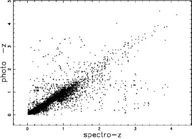
A second test fits the photometric-spectroscopic relationship with a straight line

$$y=a+bx\quad,$$ (12)

where x is the spectroscopic redshift, y is the photometric redshift, a and b two parameters to be found with the least square fit [20]. In our case $a=0.102$ , $b=0.778$ and the correlation coefficient, $r$, is 0.778.

3.3 The observed LF

A LF for galaxies is built according to the following points:

1. An upper value of redshift is chosen (i.e. $0.05$);

2. SWIRE’s galaxies are selected according to the following ranges of existence: $7\leq Log10(L/L{\hbox{$\odot$}})\leq 11$ where $L$ is the B-band luminosity;

3. We organize a histogram with bins large $\approx$ one decade;

4. We then divide the obtained frequencies by the involved comoving volume;

5. We apply the $1/V_{max}$ method because our sample is incomplete at low values of luminosity, see [21, 22, 23]. The maximum value in redshift at which a galaxy can be detected is found solving the following non linear equation

   $$f_{ave}=\frac{L_{i}}{4\pi D_{L}(z;c,H_{0},\Omega_{\rm M})^{2}}\quad,$$ (13)

   where $f_{ave}$ is the averaged flux of the sample and $L_{i}$ the luminosity of the considered bin $i$;

6. The error of the LF is evaluated as the square root of the frequencies divided by the comoving volume, as given by eqn. (10).

An example of LFs for SWIRE that are found by implementing the $1/V_{max}$ estimator, see [24], can be found in Figure 2 in [25].

3.4 Statistical tests

The merit function $\chi^{2}$ is computed as

$$\chi^{2}=\sum_{j=1}^{n}(\frac{LF_{theo}-LF_{astr}}{\sigma_{LF_{astr}}})^{2}\quad,$$ (14)

where $n$ is the number of bins for the LF of the galaxies, the index $theo$ stands for ‘theoretical’, the index $astr$ stands for ‘astronomical’ and $\sigma_{LF_{astr}}$ is the error in the LF. The reduced merit function $\chi_{red}^{2}$ is evaluated by

$$\chi_{red}^{2}=\chi^{2}/NF\quad,$$ (15)

where $NF=n-k$ is the number of degrees of freedom and $k$ is the number of parameters. The goodness of the fit can be expressed by the probability $Q$, see Equation 15.2.12 in [20], which involves the number of degrees of freedom and $\chi^{2}$. According to [20], the fit “may be acceptable” if $Q\geq 0.001$. The Akaike information criterion (AIC), see [26], is defined by

$$AIC=2k-2ln(L)\quad,$$ (16)

where $L$ is the likelihood function and $k$ is the number of free parameters in the model. We assume a Gaussian distribution for the errors and we also assume that the likelihood function can be derived from the $\chi^{2}$ statistic $L\propto\exp(-\frac{\chi^{2}}{2})$ where $\chi^{2}$ has been computed by Equation (14), see [27], [28]. The AIC now becomes

$$AIC=2k+\chi^{2}\quad.$$ (17)

3.5 Schechter LF

The Schechter LF of galaxies ,$\Phi$, see [13], is

$$\Phi(L;\Phi^{*},\alpha,L^{*})dL=(\frac{\Phi^{*}}{L^{*}})(\frac{L}{L^{*}})^{\alpha}\exp\bigl{(}{-\frac{L}{L^{*}}}\bigr{)}dL\quad,$$ (18)

where $\alpha$ sets the slope for low values of $L$, $L^{*}$ is the characteristic luminosity, and $\Phi^{*}$ represents the number of galaxies per $Mpc^{3}$. The normalization is

$$\int_{0}^{\infty}\Phi(L;\Phi^{*},\alpha,L^{*})dL=\rm\Phi^{*}\,\Gamma\left(\alpha+1\right)\quad,$$ (19)

where

$$\rm\Gamma\,(z)=\int_{0}^{\infty}e^{{-t}}t^{{z-1}}dt\quad,$$ (20)

is the Gamma function. The average luminosity, ${\langle L\rangle}$, is

$${\langle(\Phi(L;\Phi^{*},\alpha,L^{*})\rangle}=\rm L^{*}\,{\rm\Phi^{*}}\,\Gamma\left(\alpha+2\right)\quad.$$ (21)

An equivalent form in absolute magnitude of the Schechter LF is

$$\Phi(M;\Phi^{*},\alpha,M^{*})dM=$$

$$0.921\Phi^{*}10^{0.4(\alpha+1)(M^{*}-M)}\exp\bigl{(}{-10^{0.4(M^{*}-M)}}\bigr{)}dM\,,$$ (22)

where $M^{*}$ is the characteristic magnitude. We briefly recall the existence of the Wisconsin-Indiana-Yale-NOAO Observatory (WIYN) at Kitt Peak National Observatory.

A typical result of the Schechter LF in the case of SWIRE/WIYN $LF_{24}$, see Figure2 in [25] where the index 24 stands for $24\mu\,m$, is reported in Figure 2 with parameters as in Table 2.

Figure 2: The observed SWIRE/WIYN $LF_{24}$ for galaxies, empty stars, (data extracted by the author) and the fit by the Schechter LF.

3.6 The lognormal LF

Let $L$ be a random variable taking values $L$ in the interval $[0,\infty]$; the lognormal. The PDF, following [29] or formula (14.2)^′ in [30], is

$$PDF(L;L^{*},\sigma)=\frac{\sqrt{2}{{\rm e}^{-\frac{1}{2}\,{\frac{1}{{\sigma}^{2}}\left(\ln\left({\frac{L}{{\it L^{*}}}}\right)\right)^{2}}}}k}{2\,L\sigma\,\sqrt{\pi}}\quad,$$ (23)

where $L^{*}=\exp{\mu_{LN}}$ and $\mu_{LN}=\ln{L^{*}}$. The mean luminosity is

$$E(L;L^{*},\sigma)={\it L^{*}}\,{{\rm e}^{\frac{1}{2}\,{\sigma}^{2}}}\quad.$$ (24)

The luminosity function for galaxies, $\Phi(L;L^{*},\sigma)$, can be obtained by multiplying the lognormal PDF by $\Phi^{*}$, which is the number of galaxies per Mpc³ units

$$\Phi(L;L^{*},\sigma)=\Phi^{*}\frac{\sqrt{2}{{\rm e}^{-\frac{1}{2}\,{\frac{1}{{\sigma}^{2}}\left(\ln\left({\frac{L}{{\it L^{*}}}}\right)\right)^{2}}}}}{2\,L\sigma\,\sqrt{\pi}}\quad,$$ (25)

for further details, see [8]. The magnitude version for the lognormal LF is

$$\Phi(M;M^{*},\sigma)=0.3674\,{\frac{{\it\Phi^{*}}}{\sigma}{{\rm e}^{-0.4241\,{\frac{\left({\it M^{*}}-1.0\,{\it M}\right)^{2}}{{\sigma}^{2}}}}}}\quad,$$ (26)

where $M^{*}$ is the scaling absolute magnitude and $M$ is the absolute magnitude.

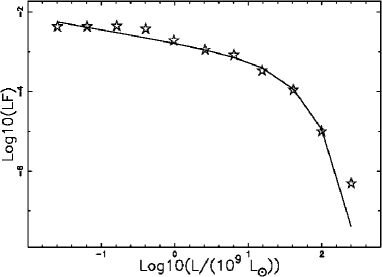
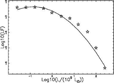
The resulting fitting curve is displayed in Figure 3, with parameters as in the second column of Table 1.

Figure 3: The observed LF for galaxies in B-band , empty stars with error bar, and the fit by the lognormal LF when the distance covers the $[0,0.05]$ range in redshift.

Table 1: Parameters and statistical tools for SWIRE LF and SWIRE/WIYN $LF_{24}$ as modeled by the lognormal LF for $z$ in $[0,0.05]$ with the SWIRE data.

Parameter	SWIRE  LF	SWIRE/WIYN $LF_{24}$
$\frac{L^{*}}{10^{9}\,L_{\hbox{$\odot$}}}$	0.696	3.25
$\sigma$	0.996	1.77
$\frac{\Phi^{*}}{Mpc^{-3}}$	0.021	0.014
Q	0	2.05 $10^{-6}$
NF	4	4
$\chi_{red}^{2}$	59.56	5.12
AIC	238.27	47.03

Table 2: Parameters and statistical tools for SWIRE LF and SWIRE/WIYN $LF_{24}$ as modeled by the Schechter LF for $z$ in $[0,0.05]$ with the SWIRE data.

Parameter	SWIRE  LF	SWIRE/WIYN $LF_{24}$
$\frac{L^{*}}{10^{9}\,L_{\hbox{$\odot$}}}$	1.035	28.46
$\alpha$	-0.02	-0.33
$\frac{\Phi^{*}}{Mpc^{-3}}$	0.02	0.0156
Q	0	$6.977\,10^{-5}$
NF	4	4
$\chi_{red}^{2}$	126	4.087
AIC	510	38.69

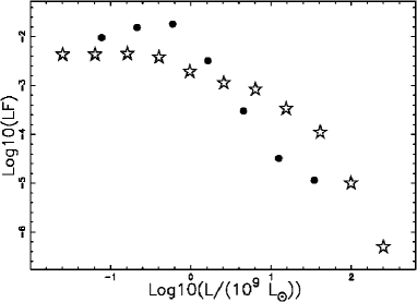
A comparison can be made with the SWIRE/WIYN 24$\mu\,m$ LF, $LF_{24}$, as reported in Figure 2 in [25] (data extracted by the author), see Figure 4.

Figure 4: SWIRE/WIYN $LF_{24}$, empty stars (data extracted by the author), and SWIRE LF in B-band, filled circles.

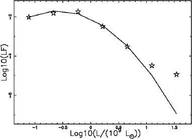
A typical result of the lognormal LF in the case of SWIRE/WIYN $LF_{24}$ is reported in Figure 5, with parameters as in the second column of Table 1.

Figure 5: The observed SWIRE/WIYN $LF_{24}$ for galaxies, empty stars, (data extracted by the author) and the fit by the lognormal LF.

4 Photometric maximum

The flux,$f$, is

$$f=\frac{L}{4\pi r^{2}}\quad,$$ (27)

where $r$ is the luminosity distance. The redshift is approximated as

$$z=z_{2,2}\quad,$$ (28)

where $z_{2,2}$ has been introduced into equation (5). The relationship between $dr$ and $dz$ is

$$dr=\frac{104306\,\left(2676.6\,z+772.8914\,{z}^{2}+846.892\right)}{\left(z+83.4793\right)^{2}\left(z+1.7548\right)^{2}}dz\quad,$$ (29)

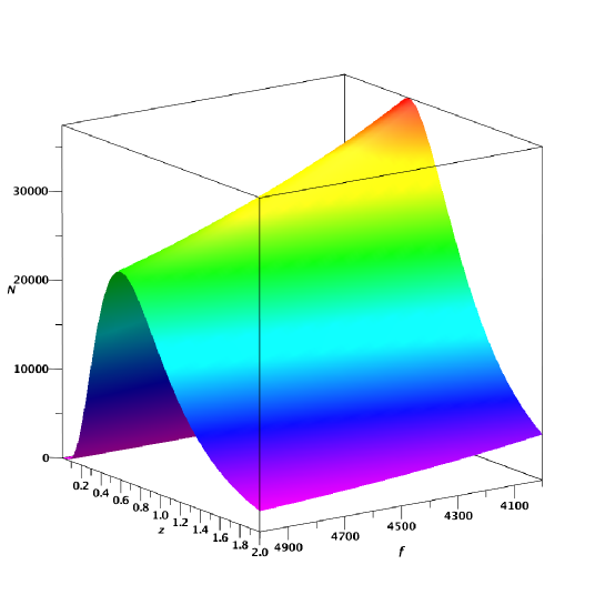
where $r$ has been defined as $D_{L,m,2,2}$ by the minimax rational approximation. The joint distribution in z and f for the number of galaxies is

$$\frac{dN}{d\Omega dzdf}=\frac{1}{4\pi}\int_{0}^{\infty}4\pi r^{2}dr\Phi(L;L^{*},\sigma)\delta\bigl{(}z-(z_{2,2})\bigr{)}\delta\bigl{(}f-\frac{L}{4\pi r^{2}}\bigr{)}\quad,$$ (30)

where $\delta$ is the Dirac delta function and $\Phi(L;L^{*},\sigma)$ has been defined in equation (25). This formula has the following explicit version

$$\frac{dN}{d\Omega dzdf}={2.92\times 10^{19}}\,{\frac{\left(z+0.6317\right)^{2}\left(z+0.001599\right)^{2}\left(z+3.1108\right)\left(z+0.35222\right)}{\left(z+83.4793\right)^{4}\left(z+1.7548\right)^{4}f\sigma}}\times$$

$${{{\rm e}^{-0.5\,{\frac{1}{{\sigma}^{2}}\left(\ln\left(1.141\,10^{13}\,{\frac{f\left(z+0.63179\right)^{2}\left(z+0.00159987\right)^{2}}{\left(z+83.4793\right)^{2}\left(z+1.75483\right)^{2}{\it L^{*}}}}\right)\right)^{2}}}}}\quad.$$ (31)

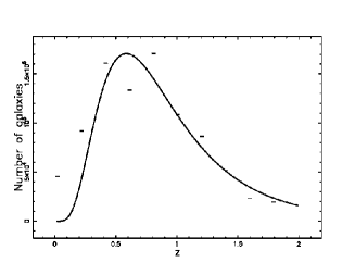
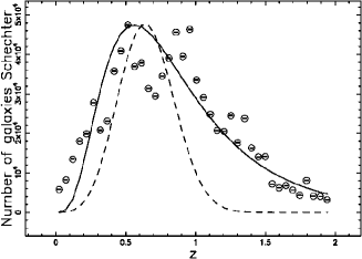
Figure 6 presents the number of galaxies that are observed in SWIRE as a function of the redshift for a given window in flux, in addition to the theoretical curve.

Figure 6: The galaxies of SWIRE in B-band with $0.00057\,L_{\hbox{$\odot$}}/Mpc^{2}\leq f\leq 10501\,L_{\hbox{$\odot$}}/Mpc^{2}$ are organized by frequency versus distance (empty circles); the error bar is given by the square root of the frequency. The maximum frequency of the observed galaxies is at $z=0.9$. The full line is the theoretical curve generated by $\frac{dN}{d\Omega drdf}$ as given by the application of the lognormal LF, which is Equation (31), and the theoretical maximum is at $z=0.57$. The parameters are $L^{*}=9\,10^{10}L_{\hbox{$\odot$}}$ and $\sigma$ =1.4  .

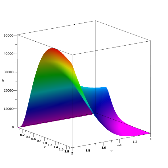
The theoretical number of galaxies is reported in Figure 7 as a function of the flux and redshift, and is reported in Figure 8 as a function of $\sigma$ and redshift.

Figure 7: The theoretical number of galaxies as a function of redshift and flux expressed in $L_{\hbox{$\odot$}}/Mpc^{2}$. The parameters are $\frac{L^{*}}{10^{9}\,L_{\hbox{$\odot$}}}=9\,10^{9}$, $\sigma=1.4$ and $\frac{\Phi^{*}}{Mpc^{-3}}=0.015$ .

Figure 8: The theoretical number of galaxies as a function of $sigma$ and redshift when $\frac{L^{*}}{10^{9}\,L_{\hbox{$\odot$}}}=9\,10^{9}$, $f=5250L_{\hbox{$\odot$}}/Mpc^{2}$ and $\frac{\Phi^{*}}{Mpc^{-3}}=0.015$ .

An analogous procedure for the joint distribution in z and f for the number of galaxies in the case of the Schechter LF derives

$$\frac{dN}{d\Omega dzdf}={8.3533\times 10^{32}}\,{\frac{\left(z+0.001599\right)^{4}\left(z+0.6317\right)^{4}{\it\Phi^{*}}\,\left(z+3.110\right)\left(z+0.3522\right)}{\left(z+83.4793\right)^{6}\left(z+1.75483\right)^{6}{\it L^{*}}}}\times$$

$${\left(1.141\,10^{13}\,{\frac{f\left(z+0.63179\right)^{2}\left(z+0.001599\right)^{2}}{\left(z+83.4793\right)^{2}\left(z+1.7548\right)^{2}{\it L^{*}}}}\right)^{\alpha}{{\rm e}^{-1.141\,10^{13}\,{\frac{f\left(z+0.631791\right)^{2}\left(z+0.001599\right)^{2}}{\left(z+83.4793\right)^{2}\left(z+1.7548\right)^{2}{\it L^{*}}}}}}}$$ (32)

Figure 9: The galaxies of SWIRE in B-band in frequencies versus redshift (empty circles). The full line is the theoretical curve generated by $\frac{dN}{d\Omega drdf}$, as given by the application of the lognormal LF, which is Equation (31), with parameters as in Figure 6. The dashed line is the theoretical curve generated by $\frac{dN}{d\Omega drdf}$, as given by the application of the Schechter LF, which is given in Equation (32), with parameters as given in Figure 6. The input parameters of the Schechter LF are $\frac{L^{*}}{10^{9}\,L_{\hbox{$\odot$}}}$=200, $\alpha$=-0.33 and $\frac{\Phi^{*}}{Mpc^{-3}}$=0.0156. The goodness of fit is $\chi^{2}=389246$ for the Schechter LF and $\chi^{2}=83970$ for the lognormal LF.

5 Conclusions

Flat cosmology In this paper, we derive an approximate relationship for the luminosity distance in spatially flat cosmology with pressure-less matter and cosmological constant, $H_{0}=70\mathrm{km\,s^{-1}\,Mpc^{-1}}$ and $\Omega_{\rm M}=0.277$, as a function of the redshift, see equation (3). We have derived the inverse relationship, the redshift as a function of the luminosity distance, see equation (5).

spectro-z vs. photo-z The differences between spectroscopic and photometric redshift, as processed from the SWIRE catalog, are characterized by a nearly zero value, -0.037, and by a great error, 0.339. This fact demands for an improvement in the derivation of the photometric redshift [31].

LF Knowledge of the comoving volume allows us to derive the astronomical LF for galaxies of the SWIRE catalog in the framework of the photometric redshift. The LF is modeled with lognormal LF, see Section 3.6, and a comparison is made with the Schechter LF, see Section 3.5. We have analyzed two observed LFs with two theoretical LFs for a total of four cases. The $\chi_{red}^{2}$ of the Schechter LF was smaller than that of the lognormal in one case over four, see Tables 1 and 2. In the case of the PM, the lognormal number of galaxies as a function of the redshift gives a better fit in respect to the Schechter fit, see $\chi^{2}$ in Figure 9.

PM

The joint distribution in the photometric redshift and in the energy flux density is modeled in the case of a flat universe and a lognormal LF, see Formula (30). The position in the redshift of the maximum for PM of galaxies at a given flux or apparent magnitude does not have an analytical expression and, therefore, is found numerically, see Figure 6.

References

- [1] M. Rowan-Robinson, E. Gonzalez-Solares, M. Vaccari, L. Marchetti, Revised SWIRE photometric redshifts, MNRAS 428 (2013) 1958–1967. arXiv:1210.3471, doi:10.1093/mnras/sts163.
- [2] G. Dalya, Z. Frei, G. Galgoczi, P. Raffai, R. S. de Souza, VizieR Online Data Catalog: GLADE catalog (Dalya+, 2016), VizieR Online Data Catalog 7275.
- [3] B. V. Karasev, Statistical genesis of a lognormal distribution as a source of properties observed in the clumping of galaxies, Pisma v Astronomicheskii Zhurnal 8 (1982) 527–534.
- [4] B. McBreen, K. J. Hurley, R. Long, L. Metcalfe, Lognormal Distributions in Gamma-Ray Bursts and Cosmic Lightning, MNRAS 271 (1994) 662. doi:10.1093/mnras/271.3.662.
- [5] H. Li, E. E. Fenimore, Log-normal Distributions in Gamma-Ray Burst Time Histories, ApJ 469 (1996) L115. arXiv:astro-ph/9607131, doi:10.1086/310275.
- [6] E. Nakar, T. Piran, New Results on the Temporal Structure of GRBs, in: E. Costa, F. Frontera, J. Hjorth (Eds.), Gamma-ray Bursts in the Afterglow Era, 2001, p. 348. arXiv:astro-ph/0103011.
- [7] K. Ioka, T. Nakamura, A Possible Origin of Lognormal Distributions in Gamma-Ray Bursts, ApJ 570 (2002) L21–L24. arXiv:astro-ph/0202053, doi:10.1086/340815.
- [8] L. Zaninetti, The Truncated Lognormal Distribution as a Luminosity Function for SWIFT-BAT Gamma-Ray Bursts, Galaxies 4 (2016) 57. arXiv:1611.01650, doi:10.3390/galaxies4040057.
- [9] K. J. Hurley, B. McBreen, M. Delaney, A. Britton, Lognormal Properties of SGR 1806-20 and Implications for Other SGR Sources, Astrophysics and Space Science 231 (1995) 81–84. arXiv:astro-ph/9508074, doi:10.1007/BF00658592.
- [10] B. McBreen, K. J. Hurley, Lognormal properties of SGR1806-20 and the possibility of a quiescent population of other SGR sources, in: C. A. Meegan, R. D. Preece, T. M. Koshut (Eds.), Gamma-Ray Bursts, 4th Hunstville Symposium, Vol. 428 of American Institute of Physics Conference Series, 1998, pp. 939–943. arXiv:astro-ph/9807218, doi:10.1063/1.55418.
- [11] J. H. Marr, Angular momentum of disc galaxies with a lognormal density distribution, MNRAS 453 (2015) 2214–2219. arXiv:1507.04515, doi:10.1093/mnras/stv1734.
- [12] J. H. Marr, Galaxy rotation curves with lognormal density distribution, MNRAS 448 (2015) 3229–3241. arXiv:1502.02949, doi:10.1093/mnras/stv216.
- [13] P. Schechter, An analytic expression for the luminosity function for galaxies., ApJ 203 (1976) 297–306.
- [14] L. Zaninetti, A new luminosity function for galaxies as given by the mass-luminosity relationship , AJ 135 (2008) 1264–1275.
- [15] L. Zaninetti, The Luminosity Function of Galaxies as modelled by the Generalized Gamma Distribution , Acta Physica Polonica B 41 (4) (2010) 729–751.
- [16] M. Bilicki, J. A. Peacock, T. H. Jarrett, et al., WISE * SuperCOSMOS Photometric Redshift Catalog: 20 Million Galaxies over 3/pi Steradians, ApJS 225 (2016) 5. arXiv:1607.01182, doi:10.3847/0067-0049/225/1/5.
- [17] J. Varela, J. Betancort-Rijo, I. Trujillo, E. Ricciardelli, The Orientation of Disk Galaxies around Large Cosmic Voids, ApJ 744 (2012) 82. arXiv:1109.2056, doi:10.1088/0004-637X/744/2/82.
- [18] I. M. H. Etherington, On the Definition of Distance in General Relativity., Philosophical Magazine 15.
- [19] R. Beck, C.-A. Lin, E. E. O. Ishida, et al., On the realistic validation of photometric redshifts, MNRAS 468 (2017) 4323–4339. doi:10.1093/mnras/stx687.
- [20] W. H. Press, S. A. Teukolsky, W. T. Vetterling, B. P. Flannery, Numerical Recipes in FORTRAN. The Art of Scientific Computing, Cambridge University Press, Cambridge, UK, 1992.
- [21] Y. Avni, J. N. Bahcall, On the simultaneous analysis of several complete samples - The V/Vmax and Ve/Va variables, with applications to quasars, ApJ 235 (1980) 694–716. doi:10.1086/157673.
- [22] S. Eales, Direct construction of the galaxy luminosity function as a function of redshift, ApJ 404 (1993) 51–62. doi:10.1086/172257.
- [23] R. S. Ellis, M. Colless, T. Broadhurst, J. Heyl, K. Glazebrook, Autofib Redshift Survey - I. Evolution of the galaxy luminosity function, MNRAS 280 (1996) 235–251. arXiv:astro-ph/9512057, doi:10.1093/mnras/280.1.235.
- [24] M. Schmidt, Space Distribution and Luminosity Functions of Quasi-Stellar Radio Sources, ApJ 151 (1968) 393. doi:10.1086/149446.
- [25] N. Onyett, S. Oliver, G. Morrison, F. Owen, F. Pozzi, D. Carson, SWIRE Team, The 24m Luminosity Function of spectroscopic SWIRE sources from the Lockman Validation Field, in: L. Armus, W. T. Reach (Eds.), Astronomical Society of the Pacific Conference Series, Vol. 357 of Astronomical Society of the Pacific Conference Series, Astronomical Society of the Pacific, 2006, p. 275. arXiv:astro-ph/0503444.
- [26] H. Akaike, A new look at the statistical model identification, IEEE Transactions on Automatic Control 19 (1974) 716–723.
- [27] A. R. Liddle, How many cosmological parameters?, MNRAS 351 (2004) L49–L53.
- [28] W. Godlowski, M. Szydowski, Constraints on Dark Energy Models from Supernovae, in: M. Turatto, S. Benetti, L. Zampieri, W. Shea (Eds.), 1604-2004: Supernovae as Cosmological Lighthouses, Vol. 342 of Astronomical Society of the Pacific Conference Series, Astronomical Society of the Pacific, 2005, pp. 508–516.
- [29] M. Evans, N. Hastings, B. Peacock, Statistical Distributions - third edition, John Wiley & Sons Inc, New York, 2000.
- [30] N. L. Johnson, S. Kotz, N. Balakrishnan, Continuous univariate distributions. Vol. 1. 2nd ed., Wiley , New York, 1994.
- [31] J. Y. H. Soo, B. Moraes, B. Joachimi, W. Hartley, O. Lahav, A. Charbonnier, M. Makler, M. E. S. Pereira, J. Comparat, T. Erben, A. Leauthaud, H. Shan, L. Van Waerbeke, Morpho-z: improving photometric redshifts with galaxy morphology, MNRAS 475 (2018) 3613–3632. arXiv:1707.03169, doi:10.1093/mnras/stx3201.