Low-Rank Phase Retrieval via Variational Bayesian Learning

Abstract

In this paper, we consider the problem of low-rank phase retrieval whose objective is to estimate a complex low-rank matrix from magnitude-only measurements. We propose a hierarchical prior model for low-rank phase retrieval, in which a Gaussian-Wishart hierarchical prior is placed on the underlying low-rank matrix to promote the low-rankness of the matrix. Based on the proposed hierarchical model, a variational expectation-maximization (EM) algorithm is developed. The proposed method is less sensitive to the choice of the initialization point and works well with random initialization. Simulation results are provided to illustrate the effectiveness of the proposed algorithm.

I Introduction

Phase retrieval has attracted a lot of interest for its practical significance in many applications, including X-ray crystallography [1, 2], optics [3], astronomy [4], diffraction imaging [5], acoustics [6], quantum mechanics [7] and quantum information [8], etc. In these applications, the phase information of measurements is difficult to obtain or completely missing, and one hope to recover the unknown signal from only the intensity of the measurements. The problem of recovering a complex signal $\boldsymbol{x}\in\mathbb{C}^{n}$ from magnitude-only measurements $\boldsymbol{y}\in\mathbb{R}^{m}$ can be cast as

$$\boldsymbol{y}=|\boldsymbol{\Phi}\boldsymbol{x}|$$ (1)

where $\boldsymbol{\Phi}\in\mathbb{C}^{m\times n}$ is a known complex measurement matrix.

A variety of phase retrieval algorithms have been proposed over the past few years. One of the earliest works on phase retrieval is the Gerchberg-Saxton algorithm [9], which is based on alternating projection and iterates between the unknown phases of the measurements and the unknown signals. In [10], an alternating minimization technique with spectral initialization was developed. Recently, a convex relaxation-based method which enjoys a nice theoretical guarantee, named PhaseLift, was proposed for phase retrieval in [11]. PhaseLift transforms phase retrieval into a semidefinite program via convex relaxation. But, in the meanwhile, the signal of interest is lifted to a high dimensional space and thus the PhaseLift incurs a higher computational complexity. To avoid this drawback, nonconvex phase retrieval algorithms that directly work on the original signal space were developed, e.g. alternating minimization algorithm [10], Wirtinger flow algorithm [12] and its variants [13, 14, 15, 16, 17, 18, 19, 20], Almost all of these nonconvex methods require a sufficiently accurate initial point to guarantee to find a globally optimal solution. One exception is the gradient descent method with random initialization proposed in [21], which works as long as the sample complexity exceeds $m\gtrsim n\textrm{poly}\log(n)$. More recently, a non-lifting convex relaxation-based method, called PhaseMax [22, 23, 24] was proposed for phase retrieval, which relaxed the nonconvex equality constraints in (1) to convex inequality constraints, and solved a linear program in the natural parameter space.

In recent years, signals with more complex structures have been considered in phase retrieval problems. For example, in many applications, the signal of interest is sparse or approximately sparse, and this sparse structure can be utilized to significantly reduce the sample complexity for exact phase recovery [25, 26, 27, 28, 29, 30, 31, 32, 33, 34, 35]. In some other applications, one may collect intensity measurements of a time-varying signal at different time instants, thus resulting in a multiple measurement vector (MMV) model. Due to the temporal correlation between different time instants, the signal of interest in a matrix form usually exhibits a low-rank structure [36]. Such a low-rank phase retrieval problem was firstly introduced in [36], where an alternating minimization method was developed. In this paper, we address the low-rank phase retrieval problem from a Bayesian perspective. In particular, we propose a hierarchical prior model for low-rank phase retrieval, in which a Gaussian-Wishart hierarchical prior originally introduced in [37] is employed to promote the low-rankness of the matrix. Based on the hierarchical Bayesian model, a variational expectation-maximization (EM) algorithm is developed with phase information treated as unknown deterministic parameters. The proposed method is The proposed method is less sensitive to the choice of the initialization point and works well with random initialization. Simulation results show that our method is capable of obtaining efficient and robust results.

The rest of the paper is organized as follows. In Section II, a hierarchical Gaussian prior model for low-rank phase retrieval is introduced. Based on this hierarchical model, a variational Bayesian learning method is developed in Section III. Simulation results are provided in Section IV, followed by concluding remarks in Section V.

II Bayesian Modeling

We consider a low-rank phase retrieval problem which was firstly introduced in [36]. Suppose we have a low-rank matrix $\boldsymbol{X}\triangleq[\boldsymbol{x}_{1}\phantom{0}\ldots\phantom{0}\boldsymbol{x}_{M}]\in\mathbb{C}^{N\times M}$ with its rank $r\ll\min\{N,M\}$. For each column $\boldsymbol{x}_{m}$ of the low-rank matrix, we can collect $P$ non-linear intensity measurements of the form

$$y_{p,m}=|\boldsymbol{a}_{p,m}^{H}\boldsymbol{x}_{m}+w_{p,m}|,\quad p=1,\ldots,P,\;\;m=1,\ldots,M$$ (2)

where $\boldsymbol{a}_{p,m}\in\mathbb{C}^{N}$ is the measurement vector, and $w_{p,m}$ denotes the additive noise. The problem of interest is to recover the low-rank matrix $\boldsymbol{X}$ from the $P\times M$ phaseless measurements $\{y_{p,m}\}$. Since we only have the magnitude measurements, each column of the low-rank matrix, $\boldsymbol{x}_{m}$, can only be recovered up to a phase ambiguity. Naturally, this low-rank phase retrieval problem can be formulated as

$$\min_{\boldsymbol{X}}\quad \text{rank}(\boldsymbol{X})$$

s.t. $$\boldsymbol{y}_{m}=|\boldsymbol{A}_{m}\boldsymbol{x}_{m}+\boldsymbol{w}_{m}|\quad\forall m$$ (3)

where $\boldsymbol{y}_{m}\triangleq[y_{1,m}\phantom{0}\ldots\phantom{0}y_{P,m}]^{T}$, $\boldsymbol{w}_{m}\triangleq[w_{1,m}\phantom{0}\ldots\phantom{0}w_{P,m}]^{T}$, and $\boldsymbol{A}_{m}\triangleq[\boldsymbol{a}_{1,m}\phantom{0}\ldots\phantom{0}\boldsymbol{a}_{P,m}]^{H}$. The optimization (3), however, is difficult to solve due to its non-convexity. In this paper, we consider modeling the low-rank phase retrieval problem within a Bayesian framework. To facilitate our modeling, similar to [38], we introduce a set of deterministic parameters $\{\theta_{p,m}\}$, where $\theta_{p,m}\in[0,2\pi)$ represents the missing phase of the observation $\tilde{y}_{p,m}\triangleq\boldsymbol{a}_{p,m}^{H}\boldsymbol{x}_{m}+w_{p,m}$. Therefore we can write

$$y_{p,m}=e^{-j\theta_{p,m}}(\boldsymbol{a}_{p,m}^{H}\boldsymbol{x}_{m}+w_{p,m})\quad\forall p,\forall m$$ (4)

and the measurements in a vector form can be written as

$$\boldsymbol{y}_{m}=\boldsymbol{D}_{m}(\boldsymbol{A}_{m}\boldsymbol{x}_{m}+\boldsymbol{w}_{m})\quad\forall m$$ (5)

where

$$\boldsymbol{D}_{m}\triangleq\text{diag}(e^{-j\theta_{1,m}},\ldots,e^{-j\theta_{P,m}})$$ (6)

We assume entries of $\boldsymbol{w}_{m}$ are independent and identically distributed (i.i.d.) random variables following a Gaussian distribution with zero mean and variance $\beta^{-1}$. To learn $\beta$, we place a Gamma hyperprior over $\beta$, i.e.

$$p(\beta)=\text{Gamma}(\beta|a,b)=\Gamma(a)^{-1}b^{a}\beta^{a-1}e^{-b\beta}$$ (7)

where $\Gamma(a)=\int_{0}^{\infty}t^{a-1}e^{-t}dt$ is the Gamma function. The parameters $a$ and $b$ are set to be small values, e.g. $10^{-10}$, which makes the Gamma distribution a non-informative prior.

To promote a low-rank solution of $\boldsymbol{X}$, we place a two-layer hierarchical Gaussian prior [37] on $\boldsymbol{X}$. It was shown in [37] this two-layer hierarchical Gaussian prior model has the potential to encourage a low-rank solution. Specifically, in the first layer, the columns of $\boldsymbol{X}$ are assumed mutually independent and follow a common Gaussian distribution:

$$p(\boldsymbol{X}|\boldsymbol{\Sigma})=\prod\limits_{m=1}^{M}p(\boldsymbol{x}_{m}|\boldsymbol{\Sigma})=\prod\limits_{m=1}^{M}\mathcal{N}(\boldsymbol{x}_{m}|\boldsymbol{0},\boldsymbol{\Sigma}^{-1})$$ (8)

where $\boldsymbol{\Sigma}\in\mathbb{C}^{N\times N}$ is the precision matrix. The second layer specifies a Wishart distribution as a hyperprior over the precision matrix $\boldsymbol{\Sigma}$:

$$p(\boldsymbol{\Sigma})\propto |\boldsymbol{\Sigma}|^{\frac{\nu-M-1}{2}}\exp(-\frac{1}{2}\text{tr}(\boldsymbol{W}^{-1}\boldsymbol{\Sigma}))$$ (9)

where $\nu$ and $\boldsymbol{W}\in\mathbb{R}^{N\times N}$ denote the degrees of freedom and the scale matrix of the Wishart distribution, respectively. For the standard Wishart distribution, $\nu$ is an integer which satisfies $\nu>N-1$. Nevertheless, if an improper prior is allowed [40], the choice of $\nu$ can be more flexible and relaxed as $\nu>0$.

For clarity, we plot the graphical model for our low-rank phase-retrieval problem in Fig. 1.

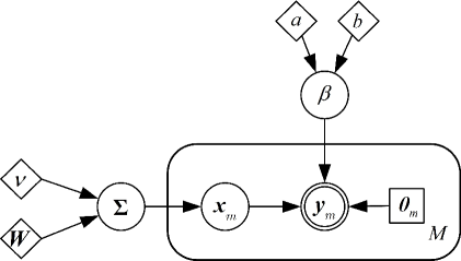
Figure 1: Graphical model for proposed Bayesian low-rank phase-retrieval method, in which double circles denote the observable variable, single circles denote the hidden variable, and the boxes denote deterministic hyperparameters, and the diamonds denote pre-specified hyperparameters

III Variational Bayesian Inference

III-A Review of The Variational Expectation Maximization Methodology

We first provide a brief review of the variational expectation maximization methodology (VEM). More details about the VEM can be found in [41]. In a probabilistic model, let $\boldsymbol{t}$, $\boldsymbol{z}$ and $\boldsymbol{\theta}$ denote the observed data, the hidden variables and the deterministic parameters, respectively. It is well-known that we can decompose the log-likelihood function into sum of two following terms [41]

$$\ln p(\boldsymbol{t;\boldsymbol{\theta}})=L(q;\boldsymbol{\theta})+\text{KL}(q||p)$$ (10)

where

$$L(q;\boldsymbol{\theta})=\int q(\boldsymbol{z})\ln\frac{p(\boldsymbol{t},\boldsymbol{z};\boldsymbol{\theta})}{q(\boldsymbol{z})}d\boldsymbol{z}$$ (11)

and

$$\text{KL}(q||p)=-\int q(\boldsymbol{z})\ln\frac{p(\boldsymbol{z}|\boldsymbol{t};\boldsymbol{\theta})}{q(\boldsymbol{z})}d\boldsymbol{z}$$ (12)

where $q(\boldsymbol{z})$ is an arbitrary probability density function, $\text{KL}(q||p)$ is the Kullback-Leibler divergence between $p(\boldsymbol{z}|\boldsymbol{t};\boldsymbol{\theta})$ and $q(\boldsymbol{z})$. Since $\text{KL}(q||p)\geq 0$, $L(q;\boldsymbol{\theta})$ is a lower bound on $\ln p(\boldsymbol{t};\boldsymbol{\theta})$. It is usually difficult to directly maximize the log-likelihood function $\ln p(\boldsymbol{t};\boldsymbol{\theta})$. To address this difficulty, we, alternatively, search for $\boldsymbol{\theta}$ by maximizing its lower bound $L(q;\boldsymbol{\theta})$. This naturally leads to a variational EM methodology, which alternatively maximizes $L(q;\boldsymbol{\theta})$ with respect to $q(\boldsymbol{z})$ and $\boldsymbol{\theta}$. First, given the current estimate of $q^{\text{old}}(\boldsymbol{z})$, we update $\boldsymbol{\theta}$ via maximizing $L(q^{\text{old}};\boldsymbol{\theta})$, which is referred to as the maximization step. Then, given the current estimate of $\boldsymbol{\theta}^{\text{old}}$, we maximize $L(q;\boldsymbol{\theta}^{\text{old}})$ with respect to $q(\boldsymbol{z})$, which is referred to as the expectation step. Specifically, to facilitate the optimization of $L(q;\boldsymbol{\theta}^{\text{old}})$, a factorized form of $q(\boldsymbol{z})$ is assumed [41], i.e. $q(\boldsymbol{z})=\prod_{i}q_{i}(z_{i})$. The maximization of $L(q;\boldsymbol{\theta}^{\text{old}})$ with respect to $q(\boldsymbol{z})$ can be conducted in an alternating fashion for each latent variable, which yields [41]

$$q_{i}(z_{i})=\frac{\exp(\langle\ln p(\boldsymbol{t},\boldsymbol{z};\boldsymbol{\theta}^{\text{old}})\rangle_{k\neq i})}{\int\exp(\langle\ln p(\boldsymbol{t},\boldsymbol{z};\boldsymbol{\theta}^{\text{old}})\rangle_{k\neq i})d\theta_{i}}$$ (13)

where $\langle\cdot\rangle_{k\neq i}$ denotes an expectation with respect to the distributions $q_{i}(\theta_{i})$ for all $k\neq i$.

III-B Proposed Algorithm

We now proceed to perform Bayesian inference for our problem. Let $\boldsymbol{z}\triangleq\{\boldsymbol{X},\boldsymbol{\Sigma},\beta\}$ denote the hidden variables, and $\boldsymbol{\theta}\triangleq\{\theta_{p,m}\}$ denote the unknown deterministic parameters in our graphical model. Our objective is to obtain an estimate of $\boldsymbol{\theta}$, along with the approximate posterior distribution for $\boldsymbol{z}$. We assume that $q(\boldsymbol{z})$ has a factorized form over the hidden variables $\{\boldsymbol{X},\boldsymbol{\Sigma},\beta\}$, i.e.

$$q(\boldsymbol{z})=q_{X}(\boldsymbol{X})q_{\Sigma}(\boldsymbol{\Sigma})q_{\beta}(\beta)$$ (14)

As discussed in the previous subsection, the maximization of the lower bound $L(q;\boldsymbol{\theta})$ can be conducted in an alternating fashion, which leads to

E-step:

$$\ln{q_{X}(\boldsymbol{X})}=\langle\ln{p(\boldsymbol{Y}|\boldsymbol{X},\beta)p(\boldsymbol{X}|\boldsymbol{\Sigma})}\rangle_{q_{\Sigma}(\boldsymbol{\Sigma})q_{\beta}(\beta)}+const,$$

$$\ln{q_{\Sigma}(\boldsymbol{\Sigma})}=\langle\ln{p(\boldsymbol{X}|\boldsymbol{\Sigma})p(\boldsymbol{\Sigma})}\rangle_{q_{X}(\boldsymbol{X})q_{\beta}(\beta)}+const,$$

$$\ln{q_{\beta}(\beta)}=\langle\ln{p(\boldsymbol{Y}|\boldsymbol{X},\beta)p(\beta)}\rangle_{q_{\Sigma}(\boldsymbol{\Sigma})q_{X}(\boldsymbol{X})}+const,$$

M-step:

$$\boldsymbol{\theta}=\arg\max_{\boldsymbol{\theta}}\langle\ln{p(\boldsymbol{Y},\boldsymbol{X},\boldsymbol{\Sigma},\beta;\boldsymbol{\theta})}\rangle_{q_{\Sigma}(\boldsymbol{\Sigma})q_{X}(\boldsymbol{X})q_{\beta}(\beta)}$$

where $\langle\rangle_{q_{1}(\cdot)...q_{K}(\cdot)}$ denotes the expectation with respect to the distributions $\{q_{k}(\cdot)\}_{k=1}^{K}$. Details of the Bayesian inference are provided next.

E-Step: Update of $q_{X}(\boldsymbol{X})$: Since columns of $\boldsymbol{X}$ are mutually independent, the approximate posterior distribution of each column can be calculated independently as

$$\ln{q_{x}(\boldsymbol{x}_{m})}$$

$$\propto\langle\ln{[p(\boldsymbol{y}_{m}|\boldsymbol{x}_{m})p(\boldsymbol{x}_{m}|\boldsymbol{\Sigma})]}\rangle_{q_{\Sigma}(\boldsymbol{\Sigma})q_{\beta}(\beta)}$$

$$\propto\langle-\beta(\boldsymbol{D}_{m}^{-1}\boldsymbol{y}_{m}-\boldsymbol{A}_{m}\boldsymbol{x}_{m})^{H}(\boldsymbol{D}_{m}^{-1}\boldsymbol{y}_{m}-\boldsymbol{A}_{m}\boldsymbol{x}_{m})-\boldsymbol{x}_{m}^{H}\boldsymbol{\Sigma}\boldsymbol{x}_{m}\rangle$$

$$\propto-\boldsymbol{x}_{m}^{H}(\langle\beta\rangle\boldsymbol{A}_{m}^{H}\boldsymbol{A}_{m}$$

$$\;\;\;\;+\langle\boldsymbol{\Sigma}\rangle)\boldsymbol{x}_{m}+\langle\beta\rangle(\boldsymbol{x}_{m}^{H}\boldsymbol{A}_{m}^{H}\boldsymbol{D}_{m}^{-1}\boldsymbol{y}_{m}+(\boldsymbol{D}_{m}^{-1}\boldsymbol{y}_{m})^{H}\boldsymbol{A}_{m}\boldsymbol{x}_{m})$$ (15)

From (15), it can be seen that $\boldsymbol{x}_{m}$ follows a Gaussian distribution

$$q_{x}(\boldsymbol{x}_{m})=\mathcal{CN}(\boldsymbol{x}_{m}|\boldsymbol{\mu}_{m},\boldsymbol{Q}_{m})$$ (16)

with its mean $\boldsymbol{\mu}_{m}$ and covariance matrix $\boldsymbol{Q}_{m}$ given as

$$\boldsymbol{\mu}_{m} =\langle\beta\rangle\boldsymbol{Q}_{m}\boldsymbol{A}_{m}^{H}\boldsymbol{D}_{m}^{-1}\boldsymbol{y}_{m}$$ (17)

$$\boldsymbol{Q}_{m} =(\langle\beta\rangle\boldsymbol{A}_{m}^{H}\boldsymbol{A}_{m}+\langle\boldsymbol{\Sigma}\rangle)^{-1}$$ (18)

E-Step: Update of $q_{\Sigma}(\boldsymbol{\Sigma})$: The approximate posterior $q_{\Sigma}(\boldsymbol{\Sigma})$ can be obtained as

$$\ln{q_{\Sigma}(\boldsymbol{\Sigma})}$$

$$\propto\langle\ln{[\prod\limits_{m=1}^{M}p(\boldsymbol{x}_{m}|\boldsymbol{\Sigma})p(\boldsymbol{\Sigma})]}\rangle_{q_{X}(\boldsymbol{X})}$$

$$\propto(\nu+M-N-1)\ln{|\boldsymbol{\Sigma}|}-\text{tr}[(\boldsymbol{W}^{-1}+\langle\boldsymbol{XX}^{H}\rangle)\boldsymbol{\Sigma}]$$ (19)

From the above equation, we see that the posterior of $\boldsymbol{\Sigma}$ follows a Wishart distribution, that is

$$q_{\Sigma}(\boldsymbol{\Sigma})=\text{Wishart}(\boldsymbol{\Sigma};\hat{\boldsymbol{W}},\hat{\nu})$$ (20)

where

$$\hat{\boldsymbol{W}} =(\boldsymbol{W}^{-1}+\langle\boldsymbol{XX}^{H}\rangle)^{-1}$$ (21)

$$\hat{\nu} =\nu+M$$ (22)

E-Step: Update of $q_{\beta}(\beta)$: The variational optimization of $q_{\beta}(\beta)$ yields

$$\ln{q_{\beta}(\beta)}$$

$$\propto\langle\ln{[\prod\limits_{m=1}^{M}p(\boldsymbol{y}_{m}|\boldsymbol{x}_{m},\beta)p(\beta)]}\rangle_{q_{X}(\boldsymbol{X})}$$

$$\propto(PM+a-1)\ln{\beta}$$

$$\;\;\;\;-(\sum\limits_{m=1}^{M}\langle\|\boldsymbol{D}_{m}^{-1}\boldsymbol{y}_{m}-\boldsymbol{A}_{m}\boldsymbol{x}_{m}\|^{2}\rangle+b)\beta$$ (23)

It is easy to verify that $q_{\beta}(\beta)$ follows a Gamma distribution

$$q_{\beta}(\beta)=\text{Gamma}(\beta|\hat{a},\hat{b})$$ (24)

where

$$\hat{a} =PM+a$$ (25)

$$\hat{b} =\sum\limits_{m=1}^{M}\langle||\boldsymbol{D}_{m}^{-1}\boldsymbol{y}_{m}-\boldsymbol{A}_{m}\boldsymbol{x}_{m}||^{2}\rangle+b$$ (26)

M-Step: Update of $\boldsymbol{\theta}$: We conduct the partial derivative of $\langle\ln{p(\boldsymbol{Y},\boldsymbol{X},\boldsymbol{\Sigma},\beta;\boldsymbol{\theta})}\rangle_{q_{\Sigma}(\boldsymbol{\Sigma})q_{X}(\boldsymbol{X})q_{\beta}(\beta)}$ with respect to $\theta_{p,m}$, which yields

$$\frac{\partial\langle\ln p(y_{p,m}|\boldsymbol{x}_{m},\beta)\rangle_{q_{X}(\boldsymbol{X})q_{\beta}(\beta)}}{\partial\theta_{p,m}}$$

$$=-\langle\beta\rangle\langle\frac{\partial|y_{p,m}e^{j\theta_{p,m}}-\boldsymbol{a}_{p,m}^{H}\boldsymbol{x}_{m}|^{2}}{\partial\theta_{p,m}}\rangle$$

$$=-\langle\beta\rangle\langle\frac{\partial(y_{p,m}e^{j\theta_{p,m}}-\boldsymbol{a}_{p,m}^{H}\boldsymbol{x}_{m})(y_{p,m}e^{-j\theta_{p,m}}-\boldsymbol{x}_{m}^{H}\boldsymbol{a}_{p,m})}{\partial\theta_{p,m}}\rangle$$

$$=-j\langle\beta\rangle y_{p,m}e^{-j\theta_{p,m}}\langle\boldsymbol{a}_{p,m}^{H}\boldsymbol{x}_{m}-e^{2j\theta_{p,m}}\boldsymbol{x}_{m}^{H}\boldsymbol{a}_{p,m}\rangle$$

$$=-j\langle\beta\rangle y_{p,m}e^{-j\theta_{p,m}}(\boldsymbol{a}_{p,m}^{H}\boldsymbol{\mu}_{m}-e^{2j\theta_{p,m}}\boldsymbol{\mu}_{m}^{H}\boldsymbol{a}_{p,m})$$ (27)

Setting the above partial derivative equal to zero, we have

$$e^{2j\theta_{p,m}}=\frac{\boldsymbol{a}_{p,m}^{H}\boldsymbol{\mu}_{m}}{\boldsymbol{\mu}_{m}^{H}\boldsymbol{a}_{p,m}}$$ (28)

Then an estimate of $\theta_{p,m}$ can be obtained

$$\theta_{p,m}=\frac{1}{2}\arctan\Big{\{}\frac{\textrm{Im}(\boldsymbol{\varUpsilon}_{p,m})}{\textrm{Re}(\boldsymbol{\varUpsilon}_{p,m})}\Big{\}}$$ (29)

where $\boldsymbol{\varUpsilon}_{p,m}\triangleq\frac{\boldsymbol{a}_{p,m}^{H}\boldsymbol{\mu}_{m}}{\boldsymbol{\mu}_{m}^{H}\boldsymbol{a}_{p,m}}$, $\textrm{Im}(.)$ and $\textrm{Re}(.)$ denote the imaginary and real parts of $(.)$, respectively.

For clarity, we summarize our algorithm as follows.

Algorithm 1: LRPR-Variational EM

while not converge do

E-step:

Update $q_{x}(\boldsymbol{X})$ via (16) with $q_{\Sigma}(\boldsymbol{\Sigma})$ and $q_{\beta}(\beta)$ fixed;

Update $q_{\Sigma}(\boldsymbol{\Sigma})$ via (20) with $q_{x}(\boldsymbol{X})$ and $q_{\beta}(\beta)$ fixed;

Update $q_{\beta}(\beta)$ via (24) with $q_{x}(\boldsymbol{X})$ and $q_{\Sigma}(\boldsymbol{\Sigma})$ fixed;

M-step:

Estimate $\boldsymbol{\theta}$ via (28).

end while

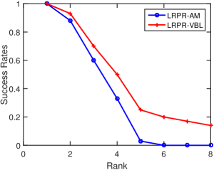
(a) $P=500$

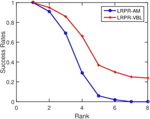
(b) $P=600$

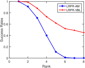
(c) $P=700$

Figure 2: Success rates of respective algorithms vs. the rank of the low-rank matrix $r$.

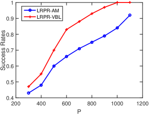
(a) $r=3$

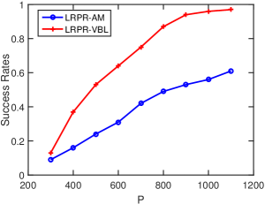
(b) $r=4$

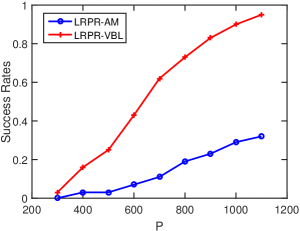
(c) $r=5$

Figure 3: Success rates of respective algorithms vs. the number of measurements $P$.

III-C Computational Complexity

The proposed algorithm requires to calculate the inverse of a matrix, i.e. (18), at each iteration. Its computational complexity scales cubically in the dimensional of the matrix, which limits its application to large-scale problems. To address this issue, a conjugate gradient method [42] can be used to significantly speed-up the numerical solution of the $n\times n$ linear system, which can be straightforwardly applied to solve (18). Besides, a recent work studies the low complexity sparse Bayesian learning algorithm [43], where the expectation step is replaced by an approximate message passing algorithm [44, 45] to reduce the computation complexity. In [37], an inverse-free Bayesian algorithm was developed via relaxed evidence lower bound maximization. The idea can also be applied to our problem to circumvent the cumbersome matrix inversion operations.

IV Simulation Results

In this section, simulation results are provided to illustrate the effectiveness of our proposed method (referred to as LRPR-VBL). The parameters used in our method are set to $a=b=v=10^{-10}$, $\boldsymbol{W}=10^{10}\boldsymbol{I}$, as suggested in [37]. We compare our method with the state-of-the-art low-rank phase retrieval algorithm (referred to as LRPR-AM) [36] which performs the low-rank phase retrieval via an alternating minimization strategy. To provide a fair comparison, both methods employ a same spectral initialization scheme which was introduced in [36].

We first examine the performance of respective algorithms under different choices of rank $r$. We randomly generate a rank-$r$ matrix $\boldsymbol{X}$ of size $100\times 100$ by multiplying two matrices $\boldsymbol{E}\in\mathbb{C}^{100\times r}$ and $\boldsymbol{F}\in\mathbb{C}^{r\times 100}$. The entries of $\boldsymbol{E}$ and $\boldsymbol{F}$ are sampled from a circularly-symmetric complex normal distribution. A set of measurement matrices $\{\boldsymbol{A}_{m}\}_{m=1}^{100}$ are produced with each of them is of size $P\times 100$. Entries of the measurement matrices are independent and follow a circularly-symmetric complex normal distribution. Fig. 2 plots the success rates vs. the rank $r$ of the low-rank matrix $\boldsymbol{X}$, where we set $P=500$, $P=600$ and $P=700$, respectively. Results are averaged over 100 independent trails. A trail is considered to be successful if the relative error of the recovery is less than 0.1, and we defined the relative error as

$$\text{RE}=\frac{\sum_{m=1}^{M}\min\limits_{\phi_{m}}||\boldsymbol{x}_{m}-e^{j\phi_{m}}\hat{\boldsymbol{x}}_{m}||^{2}}{||\boldsymbol{X}||^{2}_{F}}$$ (30)

From Fig. 2, we see that our proposed method presents a clear advantage over the LRPR-AM. This performance improvement is probably due to the fact that the EM algorithm, compared to the alternating minimization technique, is less prone to being trapped in undesirable local minima.

Next, we generate a matrix whose rank is fixed to be $r$. The success rates of respective methods as a function of the number of measurements, $P$, are plotted in Fig. 3, in which $r$ is set to $3$, $4$ and $5$, respectively. From Fig. 3, we see that to attain a same success recovery rate, our proposed method needs fewer measurements than the LRPR-AM method, which, again, demonstrates superiority of our proposed method.

Random initialization is a much simpler procedure and model-agnostic, which impels its wide use in practice. This raises an interesting question that whether our proposed LRPR-VBL algorithm with random initialization is still effective. We consider a setting similar to our previous experiment, and the initialization point is chosen uniformly random. LRPR-VBL+rand algorithm and LRPR-AM+rand stand for LRPR-VBL algorithm with random initialization and LRPR-AM algorithm with random initialization, respectively. We fix the dimension $P=1200$ and change the rank from $1$ to $7$. For each rank, we randomly generate the sampling vector $\boldsymbol{a}_{p,m}\sim\mathcal{CN}(\boldsymbol{0},\boldsymbol{I})$ in (2). Results are averaged over $50$ independent trials. As we can see from Fig. 4, our proposed method LRPR-VBL suffers from a certain amount of performance loss when the initialization point is chosen randomly. But it still performs better than the LRPR-AM method which completely fails with random initialization points. This implies that our proposed LRPR-VBL algorithm is less sensitive to the choice of the initialization point.

V Conclusions

The problem of low-rank phase retrieval was studied in this paper. To estimate a complex low-rank matrix from magnitude-only measurements, we proposed a hierarchical prior model, in which a Gaussian-Wishart hierarchical prior is placed on the underlying matrix to promote the low-rankness. Based on this hierarchical prior model, we developed a variational EM method for low-rank phase retrieval. Simulation results showed that our proposed method offers competitive performance as compared with other existing methods.

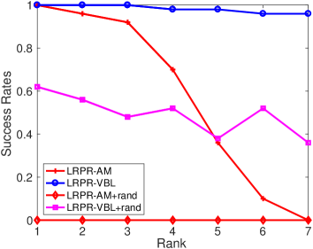
Figure 4: Success rates of respective algorithms with random initializations vs. $r$ when $P=1200$.

References

- [1] R. W. Harrison, “Phase problem in crystallography,” J. Opt. Soc. Amer. A, vol. 10, no. 5, pp. 1046–1055, 1993.
- [2] R. P. Millane, “Phase retrieval in crystallography and optics,” J. Opt. Soc. Amer. A, vol. 7, no. 3, pp. 394–411, 1990.
- [3] A. Walther, “The question of phase retrieval in optics,” J. Modern Opt., vol. 10, no. 1, pp. 41–49, 1963.
- [4] C. Fienup and J. Dainty, “Phase retrieval and image reconstruction for astronomy,” Image Recovery: Theory and Application, pp. 231–275, 1987.
- [5] O. Bunk, A. Diaz, F. Pfeiffer, C. David, B. Schmitt, D. K. Satapathy, and J. F. V. D. Veen, “Diffractive imaging for periodic samples: retrieving one-dimensional concentration profiles across microfluidic channels,” Acta Crystallograph. A, Found. Crystallogr.,, vol. 63, no. 4, pp. 306–314, 2007.
- [6] R. Balan, P. Casazza, and D. Edidin, “On signal reconstruction without phase,” Appl. Comput. Harmon. Anal., vol. 20, no. 3, pp. 345–356, 2006.
- [7] J. V. Corbett, “The pauli problem, state reconstruction and quantum-real numbers,” Rep. Math. Phys., vol. 57, no. 1, pp. 53–68, 2006.
- [8] T. Heinosaari, L. Mazzarella, and M. M. Wolf, “Quantum tomography under prior information,” Commun. Math. Phys., vol. 318, no. 2, pp. 355–374, 2013.
- [9] R. W. Gerchberg, “A practical algorithm for the determination of the phase from image and diffraction plane pictures,” Optik, vol. 35, pp. 237–246, 1972.
- [10] P. Netrapalli, P. Jain, and S. Sanghavi, “Phase retrieval using alternating minimization,” in Proc. Adv. Neural Inf. Process. Syst., Dec. 2013, pp. 2796–2804.
- [11] E. J. Candés, T. Strohmer, and V. Voroninski, “Phaselift: Exact and stable signal recovery from magnitude measurements via convex programming,” Commun. Pure Appl. Math., vol. 66, no. 8, pp. 1241–1274, 2013.
- [12] E. J. Candés, X. Li, and M. Soltanolkotabi, “Phase retrieval via wirtinger flow: Theory and algorithms,” IEEE Trans. Inf. Theory, vol. 61, no. 4, pp. 1985–2007, Apr. 2015.
- [13] Y. Chen and E. Candés, “Solving random quadratic systems of equations is nearly as easy as solving linear systems,” Commun. Pure Appl. Math., vol. 70, no. 5, pp. 822–883, 2017.
- [14] Z. Yuan and H. Wang, “Phase retrieval via reweighted wirtinger flow,” Appl. opt., vol. 56, no. 9, pp. 2418–2427, 2017.
- [15] H. Zhang, Y. Zhou, Y. Liang, and Y. Chi, “A nonconvex approach for phase retrieval: Reshaped wirtinger flow and incremental algorithms,” J. Mach. Learn. Res., vol. 18, no. 1, pp. 5164–5198, 2017.
- [16] C. Ma, K. Wang, Y. Chi, and Y. Chen, “Implicit regularization in nonconvex statistical estimation: Gradient descent converges linearly for phase retrieval, matrix completion and blind deconvolution,” arXiv preprint arXiv:1711.10467, 2017.
- [17] Z. Yang, L. F. Yang, E. X. Fang, T. Zhao, Z. Wang, and M. Neykov, “Misspecified nonconvex statistical optimization for phase retrieval,” arXiv preprint arXiv:1712.06245, 2017.
- [18] G. Wang, G. B. Giannakis, and Y. C. Eldar, “Solving systems of random quadratic equations via truncated amplitude flow,” IEEE Trans. Inf. Theory, vol. 64, no. 2, pp. 773–794, Feb. 2018.
- [19] G. Wang, G. B. Giannakis, Y. Saad, and J. Chen, “Phase retrieval via reweighted amplitude flow,” IEEE Trans. Signal Process., vol. 66, no. 11, pp. 2818–2833, Jun. 2018.
- [20] S. Pinilla, J. Bacca, and H. Arguello, “Phase retrieval algorithm via nonconvex minimization using a smoothing function,” IEEE Trans. Signal Process., vol. 66, no. 17, pp. 4574–4584, Sep. 2018.
- [21] Y. Chen, Y. Chi, J. Fan, and C. Ma, “Gradient descent with random initialization: Fast global convergence for nonconvex phase retrieval,” arXiv preprint arXiv:1803.07726, 2018.
- [22] S. Bahmani and J. Romberg, “A flexible convex relaxation for phase retrieval,” Electron. J. Statist., vol. 11, no. 2, pp. 5254–5281, 2017.
- [23] T. Goldstein and C. Studer, “Phasemax: Convex phase retrieval via basis pursuit,” IEEE Trans. Inf. Theory, vol. 64, no. 4, pp. 2675–2689, Apr. 2018.
- [24] P. Hand and V. Voroninski, “An elementary proof of convex phase retrieval in the natural parameter space via the linear program phasemax,” arXiv preprint arXiv:1611.03935, 2016.
- [25] M. L. Moravec, J. K. Romberg, and R. G. Baraniuk, “Compressive phase retrieval,” in Proceedings of SPIE Wavelets XII, vol. 6701, Sept. 2007, p. 67120.
- [26] Y. Shechtman, A. Beck, and Y. C. Eldar, “GESPAR: Efficient phase retrieval of sparse signals,” IEEE Trans. Signal Process., vol. 62, no. 4, pp. 928–938, Feb. 2014.
- [27] X. Li and V. Voroninski, “Sparse signal recovery from quadratic measurements via convex programming,” SIAM J. Math. Anal., vol. 45, no. 5, pp. 3019–3033, 2013.
- [28] P. Schniter and S. Rangan, “Compressive phase retrieval via generalized approximate message passing,” IEEE Trans Signal Process., vol. 63, no. 4, pp. 1043–1055, Feb. 2015.
- [29] Y. C. Eldar, P. Sidorenko, D. G. Mixon, S. Barel, and O. Cohen, “Sparse phase retrieval from short-time fourier measurements,” IEEE Signal Process. Lett., vol. 22, no. 5, pp. 638–642, 2015.
- [30] T. T. Cai, X. Li, Z. Ma, et al., “Optimal rates of convergence for noisy sparse phase retrieval via thresholded wirtinger flow,” Ann. Statist., vol. 44, no. 5, pp. 2221–2251, 2016.
- [31] M. Iwen, A. Viswanathan, and Y. Wang, “Robust sparse phase retrieval made easy,” Appl. Comput. Harmon. Anal, vol. 42, no. 1, pp. 135–142, 2017.
- [32] R. Pedarsani, D. Yin, K. Lee, and K. Ramchandran, “Phasecode: Fast and efficient compressive phase retrieval based on sparse-graph codes,” IEEE Trans. Inf. Theory, vol. 63, no. 6, pp. 3663–3691, Jun. 2017.
- [33] G. Jagatap and C. Hegde, “Fast, sample-efficient algorithms for structured phase retrieval,” in Proc. Adv. Neural Inf. Process. Syst., 2017, pp. 4924–4934.
- [34] G. Wang, L. Zhang, G. B. Giannakis, M. Akçakaya, and J. Chen, “Sparse phase retrieval via truncated amplitude flow,” IEEE Trans. Signal Process., vol. 66, no. 2, pp. 479–491, Jan. 2018.
- [35] P. Hand, O. Leong, and V. Voroninski, “Phase retrieval under a generative prior,” arXiv preprint arXiv:1807.04261, 2018.
- [36] N. Vaswani, S. Nayer, and Y. C. Eldar, “Low-rank phase retrieval,” IEEE Trans. Signal Process., vol. 65, no. 15, pp. 4059–4074, Aug. 2017.
- [37] L. Yang, J. Fang, H. Duan, H. Li, and B. Zeng, “Fast low-rank bayesian matrix completion with hierarchical gaussian prior models,” IEEE Trans. Signal Process., vol. 66, no. 11, pp. 2804–2817, Jun. 2018.
- [38] A. Drémeau and F. Krzakala, “Phase recovery from a bayesian point of view: The variational approach,” in Proc. IEEE Int. Conf. Acoust., Speech, Signal Process. IEEE, Apr. 2015, pp. 3661–3665.
- [39] C. M. Bishop, Pattern recognition and machine learning. Springer, 2007.
- [40] P. J. Everson and C. N. Morris, “Inference for multivariate normal hierarchical models,” J. Roy. Statist. Soc. Ser. B, vol. 62, pp. 399–412, Mar. 2000.
- [41] D. G. Tzikas, A. C. Likas, and N. P. Galatsanos, “The variational approximation for bayesian inference,” IEEE Signal Process. Mag., vol. 25, no. 6, pp. 131–146, 2008.
- [42] M. Fornasier, S. Peter, S. Worm, and S. Worm, “Conjugate gradient acceleration of iteratively re-weighted least squares methods,” Comput. Opt. and Appl., vol. 65, no. 1, pp. 205–259, 2016.
- [43] M. Al-Shoukairi, P. Schniter, and B. D. Rao, “A gamp-based low complexity sparse bayesian learning algorithm,” IEEE Trans. Signal Process., vol. 66, no. 2, pp. 294–308, Jan. 2018.
- [44] D. L. Donoho, A. Maleki, and A. Montanari, “Message-passing algorithms for compressed sensing,” Proc. Nat. Acad. Sci., vol. 106, no. 45, pp. 18 914–18 919, 2009.
- [45] S. Rangan, “Generalized approximate message passing for estimation with random linear mixing,” in Proc. IEEE Int. Symp. Inf. Theory (ISIT). IEEE, 2011, pp. 2168–2172.