The Large Sky Area Multi-Object Fiber Spectroscopic Telescope (LAMOST) Quasar Survey: the Forth and Fifth Data Release

Abstract

We present the Data Release 4&5 quasar catalog from the quasar survey by Large Sky Area Multi-Object Fiber Spectroscopic Telescope (LAMOST), which includes quasars observed between September 2015 and June 2017. There are a total of 19,253 quasars identified by visual inspections of the spectra. Among them, 11,458 are independently discovered by LAMOST, in which 3296 were reported by SDSS DR12 and DR14 quasar catalog after our survey began, while the rest 8162 are new discoveries of LAMOST. We provide the emission line measurements for the H$\alpha$, H$\beta$, Mg ii and/or C iv for 18100 quasars. Since LAMOST does not have absolute flux calibration information, we obtain the monochromatic continuum luminosities by fitting the SDSS photometric data using the quasar spectra, and then estimate the black hole masses. The catalog and spectra for these quasars are available online. This is the third installment in the series of LAMOST quasar survey which has released spectra for totally $\sim 43,000$ quasars hitherto. There are 24,772 independently discovered quasars, 17,128 of which are newly discovered. In addition to the great supplement to the new quasar discoveries, LAMOST has also provided a large database (overlapped with SDSS) for investigating the quasar spectral variability and discovering unusual quasars, including changing-look quasars, with ongoing and upcoming large surveys.

1 Introduction

Quasars, as powered by the accretion onto the supermassive black holes (SMBHs) residing in the center of their host galaxies, can emit radiation in a broad range of wavelength from radio to $\gamma$-rays, and are the most luminous, long-lived celestial objects in the Universe. They are key ingredients in our understanding of the evolution of the galaxies through cosmic time (Kormendy & Ho, 2013), and can be used to probe the intergalactic medium, the large scale structure and the reionization history of the early universe (Becker et al., 2001; Fan et al., 2002, 2006; Ross et al., 2009).

Since the discovery of the first quasar (Schmidt, 1963), great efforts have been made to find larger number of quasars during the past half century (e.g., Schmidt & Green, 1983; Hewett et al., 1995; Storrie-Lombardi et al., 1996; Boyle et al., 2000; York et al., 2000). Especially, the milestone of discovering more than $10^{5}$ new quasars has been reached thanks to the advent of two large surveys in last two decades, namely, the Two-Degree Field Quasar Redshift Survey (2dF, Croom et al., 2004) and the Sloan Digital Sky Survey (SDSS, Schneider et al., 2010). With the latest data release of SDSS-IV, the total number of currently known quasars reaches more than half million (Pâris et al., 2018).

Quasars have distinct colors from most of stars and normal galaxies (Fan, 1999). So the quasar candidates for spectroscopic observations are usually selected based on their multi-color photometric data. In particular, quasars at $z<2.2$ have a UV excess that distinguishes them from most stars. For instance, both 2dF and SDSS-I/II select quasar candidates mainly based on UV/optical photometric data in the color-color diagram (Richards et al., 2002; Smith et al., 2005). However, the completeness and efficiency of this method becomes low at $2.2<z<3.5$, especially at $z=2.7$ in SDSS, as the stellar locus intersects with the region occupied by quasars in the color-color diagram (Schneider et al., 2007).

To maximize the efficiency of identifying quasars at $2.2<z<3.5$, a lot of improvements have been made. Analogous to the UV excess seen in low-redshift quasars, there is also an excess in the near infrared $K$-band for quasars at $z>2.2$ compared to stars. A method of selecting quasar candidates at $z>2.2$ using $K$-band excess based on the UKIDSS was proposed (e.g., Warren et al., 2000; Sharp et al., 2002; Lawrence et al., 2007; Maddox et al., 2008; Smail et al., 2008). By combining the optical and infrared photometric data, Wu & Jia (2010) and Wu et al. (2012) proposed effective criteria for selecting quasar candidates based on SDSS/UKIDSS and SDSS/$WISE$ colors. These methods have led to the discovery of more and more intermediate- and high-redshift quasars (e.g., Mortlock et al., 2011; Wu et al., 2013, 2015; Wang et al., 2016).

In recent years, the quasar candidates have also been searched by using various data-mining algorithms, e.g., extreme deconvolution method (XDQSO, Bovy et al., 2011), neural network combinator (Yèche et al., 2010) and Kernel Density Estimator (KDE, Richards et al., 2004, 2009), which are adopted by SDSS-III/BOSS (Ross et al., 2012). Recently, Peng et al. (2012) develop a classification system that is made up of several support vector machine (SVM) classifiers, which can be applied to search for quasar candidates from large sky surveys. In addition, the variability-based selection (Ross et al., 2012) and cross-matching with X-ray and radio data (Ai et al., 2016) are also performed as supplement for identifying quasars.

This paper presents the quasar catalog from Large Sky Area Multi-Object Fiber Spectroscopic Telescope (LAMOST) quasar survey conducted between September 2015 and June 2017. It is the third part in a series of LAMOST quasar survey paper, after the data release 1 (DR1, Ai et al., 2016, hereafter Paper I), data release 2 and 3 (DR2 and DR3, Dong et al., 2018, hereafter Paper II). In Section 2, we briefly review the candidate selections and the spectroscopic survey. The emission line measurements and black hole mass estimations are described in Section 3 and Section 4. Section 5 presents the description of the catalog and the parameters. In Section 6 we give the summary and discussions. Throughout this work a $\Lambda$-dominated cosmology is assumed with $H_{0}=70$ km s^-1 Mpc^-1, $\Omega_{\Lambda}=0.7$ and $\Omega_{\rm M}=0.3$.

2 Survey Outline

LAMOST is a quasi-meridian reflecting Schmidt telescope with an effective light-collecting aperture that varies from 3.6 m to 4.9 m (depending on the pointing direction) and a $5\arcdeg$ field of view in diameter (Wang et al., 1996; Su & Cui, 2004; Cui et al., 2012). It has $4000$ robotic fibers, with $\sim 3\arcsec$ diameter, mounted on its focal plane and connected to 16 spectrographs. Each spectrum of the target is split into two channels, red and blue, and then recorded on red and blue cameras, respectively. The blue channel is optimized for $3700-5900$ Å, and the red channel for $5700-9000$ Å, with $200$ Å overlaps between the two channels. The spectral resolution reaches $R\sim 1800$ over the entire wavelength range (see Cui et al., 2012).

After commissioning from 2009 to 2010 and the pilot survey in 2011 (Luo et al., 2012), the LAMOST regular survey was carried out from September 2012 to June 2017, which was designed to have two major components: the LAMOST Experiment for Galactic Understanding and Exploration (LEGUE) and the LAMOST ExtraGAlactic Survey (LEGAS) (Zhao et al., 2012). The data is released in yearly increments. The LAMOST quasar survey was conducted under LEGAS which covers the high Galactic latitude area in the northern sky. The quasar candidates were observed simultaneously with other type of objects from the LEGUE and LEGAS samples during the survey. The typical exposure time for each target is usually $\sim 90$ minutes which is equally divided into three exposures. The total exposure time would be adjusted according to the observation conditions, e.g. seeing. Although LEGAS used only a small fraction of the total observing time due to the weather condition and bright sky background, LAMOST has still collected useful data and identified more than 20,000 quasars, half of which are new discoveries, during the first three years. The results of the LAMOST quasar survey as released in DR1, DR2 and DR3 are presented in Paper I and II. In this paper, we present the results of the LAMOST quasar survey conducted in the forth and fifth year as released in LAMOST data release 4 (DR4) and data release 5 (DR5).

2.1 Target Selection

The details of the method used to select the targets for LAMOST quasar survey can be found in Wu & Jia (2010), Wu et al. (2012), Peng et al. (2012) and Paper I. Here we briefly review the target selection as follows.

Most of the quasar candidates for spectroscopic followup are selected based on the photometry data of SDSS (e.g., Ahn et al., 2012). Firstly, the targets are required to be point sources in SDSS images to avoid large numbers of galaxies. A faint limit of $i=20$ is adopted to avoid the too low signal-to-noise ratio, and a bright limit of $i=16$ is adopted to avoid the saturation and the cross-talk of the neighboring fibers. Then, after the correction for Galactic extinction (Schlegel et al., 1998), the SDSS point-spread function (PSF) magnitudes are used in the selection algorithm. The targets are selected mainly based on the following methods:

1. Optical-infrared colors. Although the quasars in redshift of $2.2<z<3.5$ have similar optical color as normal stars, they are usually more luminous in infrared band (e.g., Warren et al., 2000; Maddox et al., 2008). Thus the distinct optical-infrared colors could be an useful tool in selecting quasar candidates. The photometric point sources are cross-matched with the dataset from UKIDSS/Large Area Survey (Lawrence et al., 2007) and WISE all-sky data release (Wright et al., 2010). Then, the selection is made according to the location of sources in the multi-dimensional SDSS and UKIDSS/WISE color space (Wu & Jia, 2010; Wu et al., 2012). For the UKIDSS-matched sources, quasar candidates are selected with criteria of $Y-K>0.46(g-z)+0.82$ or $J-K>0.45(i-Y-0.366)+0.64$ (Wu & Jia, 2010), where $Y$, $J$, $K$ are in Vega magnitudes and $g$, $i$, $z$ are in AB magnitudes. For the WISE-matched sources, the candidates are selected with $w1-w2>0.57$ or $z-w1>0.66(g-z)+2.01$ (Wu et al., 2012), where $w1$ and $w2$ are in Vega magnitudes and $g$, $z$ are in AB magnitudes.

2. Date-mining algorithms. A mixture of heterogeneous data-mining algorithm, such as support vector machine (SVM, Peng et al., 2012), extreme deconvolution (XD, Bovy et al., 2011) and kernel-density-estimation technique (KDE, Richards et al., 2004, 2009), are also adopted in combination with the optical-infrared color selection method. We use the same SVM algorithm demonstrated in Peng et al. (2012). The XDQSO sample are identical to that provided by Bovy et al. (2011).

3. Multi-wavelength data matching. In addition to the methods mentioned above, the final input catalog of the targets for the LAMOST quasar survey are also supplemented by cross-matching the SDSS photometry with sources detected in X-ray surveys (XMM-Newton, Chandra, ROSAT) and radio survey (FIRST, NVSS). The matching radius is 3″ for FIRST, NVSS, XMM-Newton and Chandra, and 30″ for ROSAT.

In Figure 1, we present the distribution of the $i$-band magnitude and the spectrum signal-to-noise ratio (S/N) for the observed quasar candidates in the forth and fifth years of LAMOST regular survey. Here, the S/N is calculated as the median S/N per pixel in the wavelength regions of $4000-5700$ Å and $6200-9000$ Å. As can be seen, the distributions of apparent $i$-band magnitude and spectrum S/N peak at $\sim 19.4$ mag and $\sim 2.5$, respectively.

2.2 Quasar Identification

After the observations, the raw data were reduced by the LAMOST 2D pipeline. The final spectrum of each target is produced after procedures including dark and bias subtraction, flat field correction, spectral extraction, sky subtraction, wavelength calibration, merging sub-exposures and combining blue and red spectra (see Luo et al. 2015 for details). Next, the spectra were passed to the LAMOST 1D pipeline, which automatically classifies the spectra into four categories according to their object types, namely ‘STAR’, ‘GALAXY’, ‘QSO’ and ‘Unknown’, and measures the redshift if the spectrum is classified into ‘GALAXY’ or ‘QSO’ (Luo et al., 2015).

In the early data release, only $\sim 14\%$ of the observed quasar candidates of the input catalog were identified as QSO, STAR or GALAXY by pipeline, while the majority of the spectra were classified as ‘Unknown’ (Paper I). One of the main reason was that the magnitude limit of $i=20$ is too faint for the LAMOST LEGAS survey. The varying seeing due to the site conditions on one hand and the non-classical dome of the telescope on the other hand have significantly affected the spectrum quality (Yao et al., 2012; Luo et al., 2015). As a result, the identification was often limited by the poor quality of the spectrum. This can be clearly seen in DR1 (Paper I), where the pipeline ‘Unknowns’ were on average one magnitude fainter than the pipeline identified ones. The observation conditions in later years have been improved since the first year regular survey. In addition, the pipeline has been updated in identifications of the spectra. The pie plots in Figure 2 show the fractions of each type classified by pipeline among the observed quasar candidates. It is apparent that the fraction of ‘QSO’ gets higher and higher in later data releases than in the early data release (Paper I).

Figure 1: Distributions of the SDSS $i$-band PSF magnitude and the spectrum median signal-to-noise ratio (S/N) for the observed quasar candidates in forth and fifth years of LAMOST regular survey.

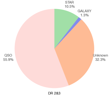
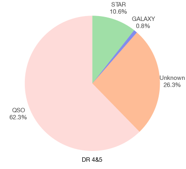
Figure 2: Fraction of objects classified as QSO, STAR, GALAXY and Unknown type by the pipeline among the targeted quasar candidates in the LAMOST regular survey.

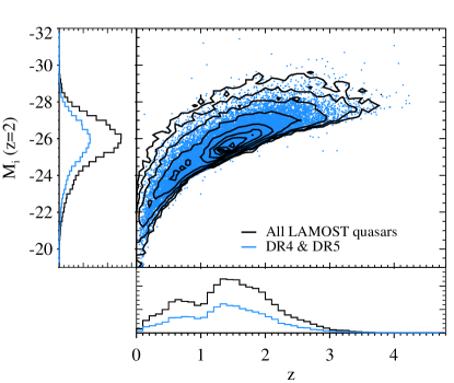
Figure 3: The absolute magnitude and redshift distribution for the visually confirmed quasars in whole LAMOST quasar survey (black) and in DR4 and DR5 of this paper (blue). The absolute magnitudes $M_{i}(z=2)$ are normalized at $z=2$.

We use a Java program ASERA (Yuan et al., 2013) to help visually inspect the observed spectra of quasar candidates as well as the spectra that are classified as QSO by the 1D pipeline but not in the input catalog of quasar candidates. The misclassified spectra are rejected or re-classified by eye. Each spectrum is inspected by two or three classifiers to check if the features of spectrum can match the quasar template. We exclude the objects with only narrow emission lines by visual inspection. Finally, the objects identified as a quasar by at least two of the classifiers were included in the final quasar catalog. The redshift of each spectrum is also inspected and estimated according to available typical quasar emission lines. We estimate the redshift based on the peak of one of the emission lines in priority order of [O iii]$\lambda 5007$, Mg ii, C iii, C iv, H$\beta$ and H$\alpha$-[N ii], when any of them are available. A flag of ‘ZWARNING=1’ will be given when there is only one emission line visible. Finally, there are 19,253 quasars with reliable identifications in DR4 and DR5. Therefore, combining the results in previous data releases (Ai et al., 2016; Dong et al., 2018), the total number of identified quasars during the first five-year regular LAMOST quasar survey reaches 43,102. LAMOST has also performed observations to search for the background quasars in the fields of M31 and M33, which are published elsewhere (e.g. Huo et al. 2010, 2013, 2015, and Huo et al. 2018 in preparation) and will not be included in this paper. Figure 3 shows our identified quasars in the luminosity-redshift space, where the luminosity is indicated using the $K$-corrected $i$-band absolute magnitudes $M_{i}(z=2)$, normalized at $z=2$ (Richards et al., 2006). As can be seen, there is a drop in the redshift distribution at $z\sim 1.0$ for DR4 and DR5, similar to the results of previous LAMOST quasar data releases (Paper I and II). The drop comes from the inefficient identification of quasars in this redshift range when the Mg ii emission line moves around the overlapping wavelength region ($\sim 6000$ Å) between the blue and red channels. The LAMOST quasar candidates were required to be point sources in our target selection (Section 2.1). It has been found that a significant fraction of quasars can be resolved up to $z\sim 0.6$ in SDSS (e.g. Matsuoka et al., 2014). Thus, LAMOST quasar sample may suffer from incompleteness at low redshift $\lesssim 0.6$.

Figure 4: Redshift differences between LAMOST and SDSS as a function of LAMOST spectrum S/N.

Among the 19,253 identified quasars in DR4 and DR5, 11,097 are known ones in SDSS DR14 quasar catalog (Pâris et al., 2018) or NED, while the rest 8162 are newly discovered quasars by LAMOST. For the sources both observed in SDSS and LAMOST, only 119 of them have redshift differences $|\Delta z|=|z_{\rm LAMOST}-z_{\rm SDSS}|>0.1$. We have visually checked the spectra of these sources and find that the differences rise from the misidentification of the redshift for LAMOST spectra. For the other objects, the uncertainty of redshift may rise for two reasons. Firstly, we estimate the redshift based on one of the typical quasar emission lines in priority orders, while SDSS redshift is based on the result of a principal component analysis and the peak of the Mg ii emission line (Pâris et al., 2018). In this case, sources of uncertainty could be line shifts relative to one another or line asymmetries. These cases are rare and deserve individual investigations. Secondly, the low S/N spectra also affect the estimation of redshift. In Figure 4, we plot the redshift differences between LAMOST and SDSS as a function of LAMOST spectrum S/N. A increasing trend of $|\Delta z|$ with decreasing S/N can be clearly seen, indicating that low S/N could be a reason for the redshift uncertainties.

As a large number of quasars in SDSS have also been observed by LAMOST, with time intervals of months to decades between SDSS and LAMOST survey, it is suitable to use SDSS and LAMOST observations to study the quasar spectral variability on both short and long timescales. For instance, it provides a large database for searching changing-look AGNs which shows appearance or disappearance of their broad emission lines (e.g., McElroy et al., 2016; MacLeod et al., 2016). Actually, LAMOST has already produced many new discoveries of this type of rare objects (Yang et al., 2018). In Figure 5 we present one such example of changing-look AGNs discovered by comparing LAMOST and SDSS observations.

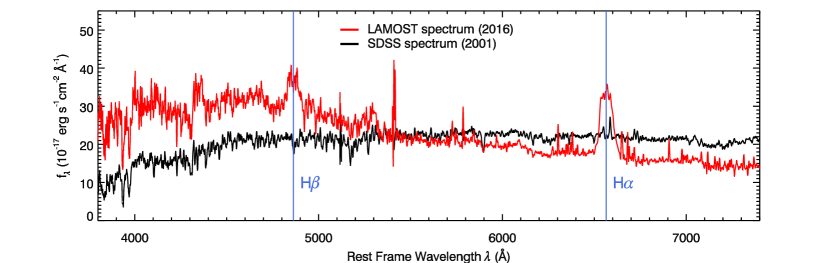
Figure 5: An example of the changing-look AGNs, J111536.57+054449.7 at $z=0.0897$ (Yang et al., 2018), discovered by cross-matching the LAMOST and SDSS observations, which shows the emergence of its broad Balmer emission lines (labeled by blue vertical line). The spectrum is corrected for the Galactic extinction and converted to the rest frame. Here, the LAMOST spectrum is not corrected for the absolute flux calibration.

3 Spectral Analysis

In this and following sections we describe the spectral analysis, the measurements of typical quasar emission lines and the estimations of black hole masses. We note that LAMOST is only equipped with spectrograph and can not provide the photometric information for the observed targets. Thus, only relative flux calibration has been applied to the released LAMOST spectra. In addition, it is difficult to find a suitable flux standard star for each spectrograph during the observations of our extra-galactic targets since they are faint and located at high Galactic latitude. So the flux calibration is very poor for these targets due to the low S/N. Therefore, we use the SDSS photometric data to estimate the continuum luminosity (see Section 4).

We fit the spectra based on IDL routines in MPFIT package (Markwardt, 2009), which performs $\chi^{2}$ minimization using Levenberg-Marquardt method. Before the fitting, each spectrum is corrected for Galactic extinction using the reddening map of Schlegel et al. (1998) with an extinction curve of $R_{V}=3.1$ (Fitzpatrick, 1999), and then transformed into the rest frame of the object using the visually inspected redshift.

Firstly, a broken power law is fitted to the spectrum in the wavelength windows of [1350, 1365] Å, [1450, 1465] Å, [1690, 1700] Å, [3790, 3800] Å, [4200, 4210] Å, [5080, 5100] Å, [5600, 5610] Å, [6120, 6130] Å  and [6900, 6910] Å. These windows are primarily chosen to avoid strong quasar emission lines listed in Vanden Berk et al. (2001). Pixels in the overlap region of LAMOST spectra (i.e. between 5700 to 6000] Å in the observed frame) between the red and blue channels are masked out during the fitting. The break of the power law is set to the value of 4661 Å at rest frame, which is similar to the value derived from the mean composite quasar spectra in Vanden Berk et al. (2001). The normalization and the indices are set as free parameters. In the next step, a local pseudo-continuum, i.e., a simple power law or a simple power law plus an Fe ii template, and line models are used to separately fit each emission line we are interested in. Here the best-fit normalization and indices from the first step are taken as the initial guess values of power law normalization and index during the fitting in the second step.

We are primarily interested in the broad H$\alpha$, H$\beta$, Mg ii and C iv emission lines, mainly because they are calibrated as virial black hole mass estimators and are the strongest broad emission lines in the available spectral range for most of the sources. The fitting procedures for each line are similar as those in Paper I (see also Dong et al. 2008 and Wang et al. 2009) and described as follows.

3.1 H$\alpha$ and H$\beta$

We fit the H$\alpha$ emission line for objects at $z\lesssim 0.33$ and H$\beta$ emission line for the quasars at $z\lesssim 0.76$. The profiles and redshifts of H$\beta$ and H$\alpha$ are not tied together since they are fitted separately. In order to fit H$\beta$, a pseudo-continuum consisting of a simple power law plus Fe ii multiplet is used to fit the spectrum in the windows [4435, 4700] Å and [5100, 5535] Å. The Fe ii template from Véron-Cetty et al. (2004) is adopted to model the optical Fe ii multiplets. Then Gaussian profiles are used to model H$\beta$+[O iii] emission lines in the range of [4600, 5100] Å after subtracting the best-fit pseudo-continuum from the spectrum. We use two Gaussians to account for the broad H$\beta$ component and one Gaussian profile to account for the narrow H$\beta$ component. The upper limit of the full width at half maximum (FWHM) for the narrow component is set to be $900\rm\,km\,s^{-1}$. It was shown in previous studies that some AGNs reveal blue wings and blueshifts in [O iii] (e.g., Greene & Ho, 2005; Komossa & Xu, 2007). So each line of the [O iii]$\lambda\lambda$4959,5007 doublet is modeled by two Gaussians, one for a line core and the other for a blueshifted wing component, and they are not tied to the H$\beta$ narrow component. The profile and redshift of each line of [O iii]$\lambda\lambda$4959,5007 doublet is tied during the fitting and their flux ratio is fixed at the theoretical value of 1:3.

For the H$\alpha$, a same pseudo-continuum is applied to fit the spectrum in windows of [6000, 6250] Å and [6800, 7000] Å. The normalization and the index of the power law are set to be free, while the parameters of the Fe ii template are fixed at the best-fit values obtained from the H$\beta$ fitting. We model the pseudo-continuum-subtracted H$\alpha$-[N ii]-[S ii] emission lines in the spectral range of [6350, 6800] Å using Gaussian profiles. The broad component of H$\alpha$ is modeled by two Gaussians, whereas [N ii]$\lambda\lambda$6548,6584, [S ii]$\lambda\lambda$6716,6731 and narrow H$\alpha$ component are modeled by a single Gaussian profile. The upper limits of the FWHM for the narrow lines are set to be $900\rm\,km\,s^{-1}$. The profile and redshift of the narrow lines are tied to each other and the relative flux ratio of [N ii]$\lambda\lambda$6548,6584 doublet is fixed at 2.96. Examples of the best-fitting results are given in Figure 6.

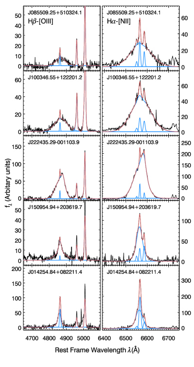
Figure 6: Sample results of the fitting procedures applied to H$\beta$+[O iii] (left panel) and H$\alpha$+[N ii] (right panel) lines. The black lines represent the extinction-corrected spectra after subtracting the best-fit pseudo-continuum. The blue lines represent the emission line model and the red lines represent the combination of models.

3.2 Mg ii

Fitting of the Mg ii and C iv emission lines are sometimes affected by the absorption features. Similar to Paper I, in order to reduce the effect of narrow absorption features, we mask out 3$\sigma$ outliers below the 20 pixel boxcar-smoothed spectrum when fitting Mg ii and C iv emission lines.

We fit Mg ii emission line for objects at $0.4\lesssim z\lesssim 2.0$. A pseudo-continuum consisting of a simple power law and ultraviolet Fe ii multiplet are used to fit the spectrum in the range of [2500, 2700] Å and [2900, 3090] Å. The Fe ii multiplet beneath the Mg ii is modeled with semi-empirical template generated by Tsuzuki et al. (2006). The best-fit pseudo-continuum is subtracted from the spectrum. Then we fit the Mg ii$\lambda\lambda$2796,2803 doublet using a similar model as in Wang et al. (2009). Each of the narrow components is modeled with a single Gaussian profile. The upper limit of FWHM is set to be $900\rm\,km\,s^{-1}$. The width and redshift of the narrow lines are tied to each other. The flux ratio is constrained between 2:1 and 1:1 (Laor et al., 1997). Each of the broad components is modeled by a truncated five-parameter Gauss-Hermite series (van der Marel & Franx 1993; see also Salviander et al. 2007). The profile, redshift and flux ratio of two broad components are constrained following the same prescription as for the narrow components. Examples of the best-fitting results are given in left panel of Figure 7.

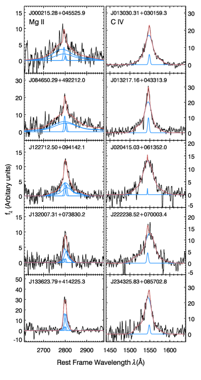
Figure 7: Same as in Figure 6 but for Mg ii doublet (left panel) and C iv (right panel) lines.

3.3 C iv

We fit the C iv emission line for objects at $1.8\lesssim z\lesssim 4.3$. Only a simple power law is fitted to the spectrum in range of [1445, 1465] Å and [1690, 1705] Å as the pseudo-continuum because Fe ii multiplet underneath C iv is very weak and it was found that fitting C iv without subtraction of Fe ii does not change the FWHM of C iv significantly (Shen et al., 2011, hereafter S11). After subtracting the best-fit continuum from the spectrum, a Gauss-Hermite series and single Gaussian profile are used to model the broad and narrow components, respectively. Similar to the fitting procedure in Paper I, we do not set upper limit for FWHM of the narrow component as there are still debates on whether or not a strong narrow component exists for the C iv line (Baskin & Laor, 2005). Examples of the best-fitting results are given in the right panel of Figure 7.

3.4 Reliability of the Fittings and Error Estimation

After the automatic procedure, we inspect the fitting results visually for each object, pick out the bad fittings and fine-tuning the fitting procedures. Finally, the results are acceptable for most of the spectra with high S/N. The bad fittings are mainly caused by low S/N or lack of good pixels. For each line, a flag of LINE_FLAG=0 is given to indicate an acceptable fitting and reliable measurement, while LINE_FLAG=-1 indicates a spurious measurement. We note that a emission line is not fitted when the fitting wavelength range is not fully covered by the observed wavelength range, or when there is not enough good pixels ($n_{\rm pixel}<100$) due to bad quality of the spectrum, or when the fitting wavelength range of the line is red-shifted to the overlapping region between the blue and red channels. In this case, we set LINE_FLAG=-9999. The broad absorption features at Mg ii and C iv also affect some of the fitting results. We give a flag of BAL_FLAG to indicate whether broad absorption features are present in the spectra by visual inspection.

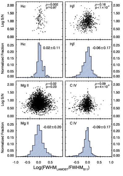
Figure 8: Comparison between the measurements of line width in this work and in Shen et al. (2011). We show the plot of $\log(\rm FWHM_{LAMOST}/FWHM_{S11})$ versus the median S/N per pixel in line-fitting region and the normalized distribution of $\log(\rm FWHM_{LAMOST}/FWHM_{S11})$ for broad H$\alpha$ (upper left), broad H$\beta$ (upper right), broad Mg ii (lower left) and total C iv (lower right) emission lines, respectively. The Spearman correlation coefficient $\rho$, $p$-values, mean value of the distribution and its standard deviation are also tabulated in the corresponding plots. Only the spectra with reliable fit (LINE_FLAG=0) are considered.

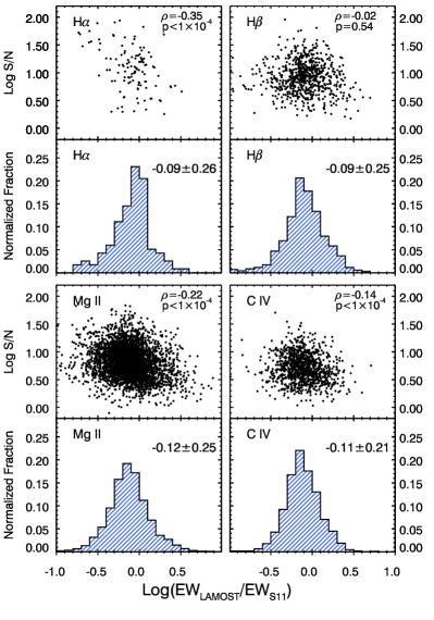
Figure 9: Same as Figure 8, but for comparison between the measurements of equivalent width in this work and in Shen et al. (2011).

In Figure 8 and 9 we plot the comparison between our fitting results and those of S11 for 5974 overlapped sources. As can be seen from the normalized distribution of $\log(\rm LAMOST/S11)$, though being generally consistent with S11, our measurement values appear to be systematically smaller (see the mean value and standard deviation of the distribution in figures). As mentioned in Paper II, the differences may be caused by different models used in the fitting. We use double Gaussians to model the broad H$\alpha$ and H$\beta$ lines, and use the Gauss-Hermite series to model the broad component of Mg ii and total C iv, while in S11 multiple Gaussians with up to three Gaussians are used to fit each broad emission lines. The templates of iron multiplet are also different, which may lead to a different pseudo-continuum.

Another possible reason is the different S/N. Figure 10 shows the normalized distributions of the median S/N per pixel in line-fitting regions for quasars in LAMOST DR4&5. The peak of the distributions are all around or below $\rm S/N=5$. We compare the median S/N per pixel of the line-fitting regions for the overlapped sources in LAMOST DR4&5 and S11 in Figure 11. The normalized distributions of $\log(S/N)_{\rm LAMOST}-\log(S/N)_{\rm S11}$ show that our spectra have significant lower S/N than those in S11 for the same object. To explore the impact of S/N on our fitting results, we also show the plots of $\log(\rm LAMOST/S11)$ versus the median S/N per pixel in line-fitting regions. In Figure 8, a trend of decreasing $\log(\rm FWHM_{LAMOST}/FWHM_{S11})$ with decreasing S/N is demonstrated by Spearman correlation test ($\rho>0$), although this trend is not significant for H$\alpha$ and Mg ii. In Figure 9, a trend of decreasing $\log(\rm EW_{LAMOST}/EW_{S11})$ with increasing S/N is demonstrated ($\rho<0$) for H$\alpha$ Mg ii and C iv. The simulation by S11 expects that the measured FWHMs and EWs are biased by less than $\pm 20\%$ for high-EW objects as S/N decreases, while the FWHMs and EWs are biased low/high by $>20\%$ as S/N decreases. However, the exact dependences of FWHMs and EWs on spectrum S/N are probably more complicated and need further explorations in the future.

To estimate the errors of the measured FWHM and EW for the broad emission lines, we assume that the measured quantities of each component of the broad emission lines follow the Gaussian distribution, of which the standard deviation is the uncertainty obtained from $\chi^{2}$ minimization. We randomly generate each component and measure the FWHM and EW of profile combined by these components. The process was repeated 1000 times and the uncertainties of FWHM and EW for the broad emission line were estimated from the 68% range of the distributions. For the narrow emission lines, the errors of the measurement is obtained from the $\chi^{2}$ minimization.

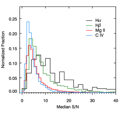
Figure 10: Normalized distributions of the median S/N per pixel around the line-fitting regions for objects with line measurements. Only the spectra with reliable fit (LINE_FLAG=0) are considered.

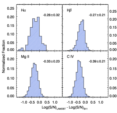
Figure 11: Comparison between the median S/N per pixel in the line-fitting region in this work and in Shen et al. (2011). The mean value and the standard deviation of distribution are tabulated in corresponding plots. Only the spectra with reliable fit (LINE_FLAG=0) are considered.

4 Continuum Luminosity and Virial Black Hole Mass

In order to estimate the continuum luminosity for LAMOST quasars, we use the SDSS $ugriz$-band photometry following the procedures in Paper I and II. Firstly, we cross-match LAMOST DR4/DR5 quasars with SDSS photometric database with a 2″-matching-radius. We extract the PSF magnitudes, correct them for Galactic extinction, and convert them into the flux densities $F_{\lambda}$ at the effective wavelength of each filter. Next, we fit the five flux densities in the rest frame with a quasar spectrum model which is composed of a broken power-law continuum emission and line emission made from the composite quasar spectra in Vanden Berk et al. (2001). During the fitting, the break of the broken power laws is fixed at 4661 Å and the normalization of the power laws is tied to the mean value of emission in ranges of [1350-1365] Å and [4200-4230] Å (Paper I). The indices of the power laws and the normalization of the line emission are set as free parameters. As results, the average power-law indices from the best-fits are found to be $\langle\alpha_{\nu}\rangle=-0.40$ ($\langle\alpha_{\lambda}\rangle=-1.60$) blueward of 4661 Å and $\langle\alpha_{\nu}\rangle=-1.65$ ($\langle\alpha_{\lambda}\rangle=-0.35$) redward of 4661 Å, which is in good agreement with those of the median composite spectra in Vanden Berk et al. (2001). Examples of the fitting results are presented in Figure 12.

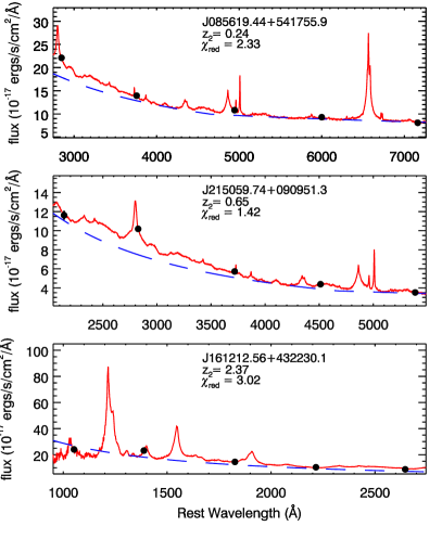
Figure 12: Examples of the model fitting to the SDSS $ugriz$-band photometry (black dots). The red solid line represents the total model spectra and the blue dashed line represents the power laws used to estimated the continuum emission.

The monochromatic continuum luminosities at 1350 Å, 3000 Å and 5100 Å are calculated from the best-fit power-law continuum, which can be used as proxies for the radius of the broad emission line region. Meanwhile, with the broad line width as a proxy for the virial velocity, the black hole masses can be estimated based on the empirical scaling relations between the virial black hole mass, the FWHM of primary emission lines and the corresponding continuum luminosities, which are calibrated using local AGNs with reverberation mapping masses (e.g., McLure & Dunlop, 2004; Vestergaard & Peterson, 2006; Wang et al., 2009). Here we estimate the virial black hole masses using relations

$$\begin{split}\log&M_{\rm BH}=\\ \log&\left\{\left[\frac{\rm FWHM(H\beta)}{\rm km\,s^{-1}}\right]^{2}\left[\frac{L_{5100}}{10^{44}\rm\,ergs\,s^{-1}}\right]^{0.5}\right\}+0.91\end{split}$$ (1)

for H$\beta$-based estimates (Vestergaard & Peterson, 2006),

$$\begin{split}\log&M_{\rm BH}=\\ \log&\left\{\left[\frac{\rm FWHM(Mg\,\text{\sc ii})}{\rm km\,s^{-1}}\right]^{1.51}\left[\frac{L_{3000}}{10^{44}\rm\,ergs\,s^{-1}}\right]^{0.5}\right\}+2.60\end{split}$$ (2)

for Mg ii-based estimates (Wang et al., 2009), and

$$\begin{split}\log&M_{\rm BH}=\\ \log&\left\{\left[\frac{\rm FWHM(C\,\text{\sc iv})}{\rm km\,s^{-1}}\right]^{2}\left[\frac{L_{1350}}{10^{44}\rm\,ergs\,s^{-1}}\right]^{0.53}\right\}+0.66\end{split}$$ (3)

for the C iv-based estimates (Vestergaard & Peterson, 2006). The FWHM of broad H$\beta$, broad Mg ii and whole C iv line are used during the estimations.

Although it’s straightforward to calculate the black hole mass using the above relations, one should bear in mind the large uncertainties of the estimates ($\gtrsim 0.4\rm\,dex$, e.g., Vestergaard & Peterson 2006; Wang et al. 2009). Figure 13 shows the distribution of the black hole masses with redshifts. It is apparent that mass estimates for the LAMOST quasars occupy the same area as those of SDSS DR7 quasars from S11.

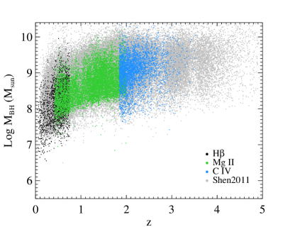
Figure 13: Black hole mass distribution along the redshift for the visually confirmed quasars of LAMOST DR4&5 with estimated black hole masses based on H$\beta$ (black), Mg ii (green) and C iv (blue). The grey dots are SDSS quasars from Shen et al. (2011).

We also note that our estimations adopt the continuum luminosities obtained from the SDSS photometry more than ten years before the LAMOST survey, which introduce additional uncertainties because the ultraviolet/optical emission of quasars varied generally with magnitudes of $0.1-0.2\rm\,mag$. To justify this effect, for the overlapped objects in LAMOST DR4&5 and S11, we compare our estimates of continuum luminosities and black hole masses with those estimated by S11 in Figure 14. It is shown that our estimates are in general agreement with S11’s results, though with systematically lower values than S11. The lower value of black hole mass may be driven by the lower S/N leading to smaller line width, as mentioned in Section 3.4.

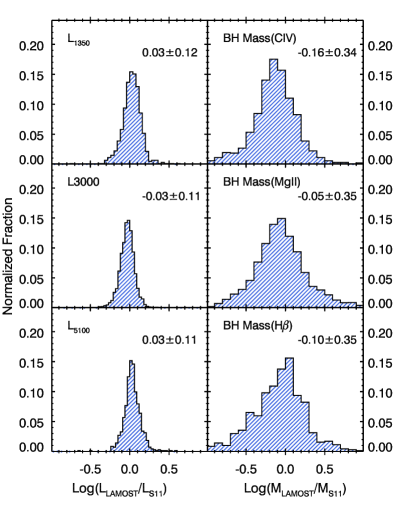
Figure 14: Left: Comparison (normalized distributions) of the continuum luminosities in this work and in Shen et al. (2011). Right: Comparison of the black hole masses estimated from H$\beta$, Mg ii and C iv emission lines in this work and in Shen et al. (2011).

5 Description of the Catalog

We give a compiled catalog for the quasars identified in LAMOST DR4&5 along with this paper. The keyword for each column are listed in Table 1 and described as below.

• Unique spectra ID.

• Target Observation date.

• LAMOST DR4&5 object name: $\rm Jhhmmss.ss+ddmmss.s$ (J2000).

• Right Ascension and Declination (in decimal degrees, J2000).

• Information of the spectroscopic observation: Modified Julian date (MJD), spectroscopic plan name (PlanID), spectrograph identification (spID), and spectroscopic fiber number (fiberID). These four numbers are unique for each spectrum named in the format of spec$-$MJD$-$planID_spID$-$fiberID.fits.

• Redshift and its flag based on visual inspections. 1$=$not robust.

• Target selection flag. This flag is a four-character string indicating how the quasar candidate is selected, in which the value of each character is a boolean value, i.e., “1” is truth and “0” is false. The first character indicates infrared-optical color selection. The second character indicates data-mining selection. The third character indicates selection based on X-ray detection. The fourth character indicates selection based on radio detection. A entry with SOURCE_FLAG=“1101” indicates that the quasar was selected by its infrared-optical color, data-mining algorithms and radio detection. A entry with SOURCE_FLAG=“0000” means the object is not included in LAMOST LEGAS quasar survey sample but identified as quasar.

• $M_{i}(z=2)$: absolute i-band magnitude. K-corrected to $z=2$ following Richards et al. (2006).

• Number of spectroscopic observations for the quasar. When there are more than one observation for the object, the line properties are obtained from only one of the observations in which the fiber pointing position is nearest to the position in our quasar candidate catalog.

• Median S/N per pixel in the wavelength regions of [4000-5700] Å and[6200, 9000] Å.

• Flag of broad absorption features. BAL_FLAG$=$1 indicates broad absorption features are present.

• FWHM, rest-frame equivalent width, and their uncertainties, for broad H$\alpha$, narrow H$\alpha$, [N ii]$\lambda 6584$, [S ii]$\lambda\lambda$6716,6731 emission lines.

• Rest-frame equivalent width of iron emissions in 6000-6500 Å.

• Number of good pixels and median S/N per pixel for the spectrum in region of rest-frame 6400-6765 Å.

• Flag indicates reliability of the emission line fitting results in H$\alpha$ region upon visual inspections. 0$=$reliable; -1$=$unreliable. This value is set to be $-9999$ if H$\alpha$ is not measured due to lack of good pixels in the fitting wavelength region.

• FWHM, rest-frame equivalent width, and their uncertainties, for broad H$\beta$, narrow H$\beta$, [O iii]$\lambda\lambda$5007 emission lines.

• Rest-frame equivalent width of iron emissions in 4685-4435 Å.

• Number of good pixels and median S/N per pixel for the spectrum in region of rest-frame 4750-4950 Å.

• Flag indicates reliability of the emission line fitting results in H$\beta$ region upon visual inspections. 0$=$reliable; -1$=$unreliable. This value is set to be $-9999$ if H$\beta$ is not measured due to lack of good pixels in the fitting wavelength region.

• FWHM, rest-frame equivalent width, and their uncertainties, of the whole Mg ii emission line.

• FWHM, rest-frame equivalent width, and their uncertainties, of the total broad Mg ii emission line.

• FWHM and its uncertainties of the broad and narrow Mg ii$\lambda$2796 emission lines.

• Rest-frame equivalent width of iron emissions in 2200-3090 Å.

• Number of good pixels and median S/N per pixel for the spectrum in region of rest-frame 2700-2900 Å.

• Flag indicates reliability of the emission line fitting results in Mg ii region upon visual inspections. 0$=$reliable; -1$=$unreliable. This value is set to be $-9999$ if Mg ii is not measured due to lack of good pixels in the fitting wavelength region.

• FWHM, rest-frame equivalent width, and their uncertainties, of the whole C iv emission line.

• FWHM, rest-frame equivalent width, and their uncertainties, of the broad C iv emission line.

• FWHM, rest-frame equivalent width, and their uncertainties, of the narrow C iv emission line.

• Number of good pixels and median S/N per pixel for the spectrum in region of rest-frame 1500-1600 Å.

• Flag indicates reliability of the emission line fitting results in C iv region upon visual inspections. 0$=$reliable; -1$=$unreliable. This value is set to be $-9999$ if C iv is not measured due to lack of good pixels in the fitting wavelength region.

• Wavelength power-law index, $\alpha_{\lambda}$, from $\sim$ 1300 to 4661 Å.

• Wavelength power-law index, $\alpha_{\lambda}$, from $\sim$ redward of 4661 Å.

• Reduced chi-square in SDSS photometry modeling; $-9999$ if not fitted.

• Monochromatic luminosities at 5100 Å, 3000 Å and 1350 Å.

• Virial black hole masses (in $M_{\odot}$) based on H$\beta$, Mg ii and C iv.

• Name of the quasar in SDSS quasar catalog. The LAMOST DR4&5 quasar catalog was cross-correlated with the SDSS quasar catalog (DR14, Pâris et al., 2018) using a matching radius of 3″.

• Name of the object in 2nd ROSAT all-sky survey point source catalog (2RXS, Boller et al., 2016). The LAMOST DR4&5 quasar catalog was cross-correlated with 2nd ROSAT all-sky survey point source catalog using a matching radius of 30″. The nearest point source in 2RXS was chosen.

• The background corrected source counts in full band (0.1-2.4 keV), and its error, from 2nd ROSAT all-sky survey point source catalog (Boller et al., 2016).

• The exposure time of the ROSAT measurement.

• Angular separation between the LAMOST and ROSAT source positions.

• Name of the object in XMM-Newton Serendipitous Source Catalog (3XMM-DR8, Rosen et al., 2016). The LAMOST DR4&5 quasar catalog was cross-correlated with XMM-Newton Serendipitous Source Catalog using a matching radius of 3″.

• The mean full-band (0.2-12 keV) flux, and its error, from XMM-Newton Serendipitous Source Catalog (Rosen et al., 2016).

• Angular separation between the LAMOST and 3XMM-DR8 source positions.

• FIRST peak flux density at 20 cm in units of mJy. The LAMOST DR4&5 quasar catalog was cross-correlated with FIRST survey catalog using a matching radius of 5″.

• Angular separation between LAMOST and FIRST source positions.

6 Summary

In this paper, we present the results of the LAMOST quasar survey in the 4th and 5th data release obtained from the observations which began at September 2015 and September 2016, respectively. There are a total of 19,253 visually confirmed quasars. The catalog and spectra of these quasars will be available online. Among these identified quasars, 11,458 were independently discovered by LAMOST, 3296 of which were reported in SDSS DR12/14 quasar catalog (Pâris et al., 2017, 2018) after the survey began, while the other 8162 are new discoveries of LAMOST that have not been reported before (see Figure 15). After the first five-year regular observation, the total number of identified quasars in LAMOST quasar survey reaches 43,102 hitherto (Ai et al., 2016; Dong et al., 2018, and this work). There are 24,772 independently discovered quasars by LAMOST, and 17,128 of them are newly discovered.

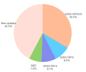
Figure 15: Visually confirmed quasars in LAMOST DR4&5. Nearly half of the sources are newly discovered.

In this work, we provide H$\alpha$, H$\beta$, Mg ii and C iv emission line properties (FWHM and equivalent width) for each quasar spectrum by performing spectral analysis. Although LAMOST is not equipped with a photometry instrument and lack the information about absolute flux calibration for the spectra, we obtain the continuum luminosity underneath the emission lines and the corresponding black hole masses by fitting the SDSS photometric data using the quasar spectra.

In addition to the great supplement to the low-to-moderate redshift quasar discoveries, LAMOST also provides a large database for investigating the quasar spectral variabilities since the LAMOST and SDSS observations were taken over roughly ten-years baseline. By comparing the LAMOST and SDSS data, more unusual quasars with, including changing-look AGNs (Yang et al., 2018) or tidal disruption events (Liu et al., 2018) may be discovered.

Table 1: Catalog format for the quasars identified in LAMOST DR4&5

Column	Name	Format	Description
1	ObsID	LONG	Unique Spectra ID
2	ObsDate	STRING	Target observation date
3	NAME	STRING	LAMOST designation hhmmss.ss+ddmmss (J2000)
4	RA	DOUBLE	Right ascension in decimal degrees (J2000)
5	DEC	DOUBLE	Declination in decimal degrees (J2000)
6	LMJD	LONG	Local Modified Julian Day of observation
7	PLANID	STRING	Spectroscopic plan name
8	SPID	LONG	Spectrograph identification
9	FIBERID	LONG	Spectroscopic fiber number
10	Z$\_$VI	DOUBLE	Redshift from visual inspection
11	ZWARNING	LONG	ZWARNING flag from visual inspection
12	SOURCE_FLAG	STRING	Target selection flag
13	MI$\_$Z2	DOUBLE	M${}_{i}(z=2)$, K-corrected to $z=2$ following Richards et al. (2006)
14	NSPECOBS	LONG	Number of spectroscopic observations
15	SNR_SPEC	DOUBLE	Median S/N per pixel of the spectrum
16	BAL_FLAG	LONG	Flag of broad absorption features
17	FWHM_BROAD_HA	DOUBLE	FWHM of broad H$\alpha$ in $\rm km\,s^{-1}$
18	ERR_FWHM_BROAD_HA	DOUBLE	Uncertainty in FWHMHα,broad
19	EW_BROAD_HA	DOUBLE	Rest-frame equivalent width of broad H$\alpha$ in Å
20	ERR_EW_BROAD_HA	DOUBLE	Uncertainty in EWHα,broad
21	FWHM_NARROW_HA	DOUBLE	FWHM of narrow H$\alpha$ in $\rm km\,s^{-1}$
22	ERR_FWHM_NARROW_HA	DOUBLE	Uncertainty in FWHMHα,narrow
23	EW_NARROW_HA	DOUBLE	Rest-frame equivalent width of narrow H$\alpha$ in Å
24	ERR_EW_NARROW_HA	DOUBLE	Uncertainty in EWHα,narrow
25	EW_NII_6584	DOUBLE	Rest-frame equivalent width of [N ii]$\lambda$6584 in Å
26	ERR_EW_NII_6584	DOUBLE	Uncertainty in EW[NII]6584
27	EW_SII_6716	DOUBLE	Rest-frame equivalent width of [S ii]$\lambda$6716 in Å
28	ERR_EW_SII_6718	DOUBLE	Uncertainty in EW[SII]6716
29	EW_SII_6731	DOUBLE	Rest-frame equivalent width of [S ii]$\lambda$6731 in Å
30	ERR_EW_SII_6731	DOUBLE	Uncertainty in EW[SII]6731
31	EW_FE_HA	DOUBLE	Rest-frame equivalent width of Fe within 6000-6500 Å in Å
32	LINE_NPIX_HA	LONG	Number of good pixels for the rest-frame 6400-6765 Å
33	LINE_MED_SN_HA	DOUBLE	Median S/N per pixel for the rest-frame 6400-6765 Å
34	LINE_FLAG_HA	LONG	Flag for the quality in H$\alpha$ fitting
35	FWHM_BROAD_HB	DOUBLE	FWHM of broad H$\beta$ in $\rm km\,s^{-1}$
36	ERR_FWHM_BROAD_HB	DOUBLE	Uncertainty in FWHMHβ,broad
37	EW_BROAD_HB	DOUBLE	Rest-frame equivalent width of broad H$\beta$ in Å
38	ERR_EW_BROAD_HB	DOUBLE	Uncertainty in EWHβ,broad
39	FWHM_NARROW_HB	DOUBLE	FWHM of narrow H$\beta$ in $\rm km\,s^{-1}$
40	ERR_FWHM_NARROW_HB	DOUBLE	Uncertainty in FWHMHβ,narrow
41	EW_NARROW_HB	DOUBLE	Rest-frame equivalent width of narrow H$\beta$ in Å
42	ERR_EW_NARROW_HB	DOUBLE	Uncertainty in EWHβ,narrow
43	FWHM_OIII_5007	DOUBLE	FWHM of [O iii]$\lambda$5007 in $\rm km\,s^{-1}$
44	ERR_FWHM_OIII_5007	DOUBLE	Uncertainty in FWHM[OIII]5007
45	EW_OIII_5007	DOUBLE	Rest-frame equivalent width of [O iii]$\lambda$5007 in Å
46	ERR_EW_OIII_5007	DOUBLE	Uncertainty in EW[OIII]5007
47	EW_FE_HB	DOUBLE	Rest-frame equivalent width of Fe within 4435-4685 Å in Å
48	LINE_NPIX_HB	LONG	Number of good pixels for the rest-frame 4750-4950 Å
49	LINE_MED_SN_HB	DOUBLE	Median S/N per pixel for the res t-frame 4750-4950 Å
50	LINE_FLAG_HB	LONG	Flag for the quality in H$\beta$ fitting
51	FWHM_MGII	DOUBLE	FWHM of the whole Mg ii emission line in $\rm km\,s^{-1}$
52	ERR_FWHM_MGII	DOUBLE	Uncertainty in FWHMMgII,whole
53	EW_MGII	DOUBLE	Rest-frame equivalent width of the whole Mg ii in Å
54	ERR_EW_MGII	DOUBLE	Uncertainty in EWMgII,whole
55	FWHM_BROAD_MGII	DOUBLE	FWHM of the whole broad Mg ii in $\rm km\,s^{-1}$
56	ERR_FWHM_BROAD_MGII	DOUBLE	Uncertainty in FWHMMgII,broad
57	EW_BROAD_MGII	DOUBLE	Rest-frame equivalent width of the whole broad Mg ii in Å
58	ERR_EW_BROAD_MGII	DOUBLE	Uncertainty in EWMgII,broad
59	FWHM_BROAD_MGII_2796	DOUBLE	FWHM of the broad Mg ii$\lambda$2796 in $\rm km\,s^{-1}$
60	ERR_FWHM_BROAD_MGII_2796	DOUBLE	Uncertainty in FWHMMgII2796,broad
61	FWHM_NARROW_MGII_2796	DOUBLE	FWHM of the narrow Mg ii$\lambda$2796 in $\rm km\,s^{-1}$
62	ERR_FWHM_NARROW_MGII_2796	DOUBLE	Uncertainty in FWHMMgII2796,narrow
63	EW_FE_MGII	DOUBLE	Rest frame equivalent width of Fe within 2200-3090 Å in Å
64	LINE_NPIX_MGII	LONG	Number of good pixels for the rest-frame 2700-2900 Å
65	LINE_MED_SN_MGII	DOUBLE	Median S/N per pixel for the rest-frame 2700-2900 Å
66	LINE_FLAG_MGII	LONG	Flag for the quality in MgII fitting
67	FWHM_CIV	DOUBLE	FWHM of the whole C iv in $\rm km\,s^{-1}$
68	ERR_FWHM_CIV	DOUBLE	Uncertainty in FWHMCIV,whole
69	EW_CIV	DOUBLE	Rest-frame equivalent width of the whole C iv in Å
70	ERR_EW_CIV	DOUBLE	Uncertainty in EWCIV,whole
71	FWHM_BROAD_CIV	DOUBLE	FWHM of the broad C iv in $\rm km\,s^{-1}$
72	ERR_FWHM_BROAD_CIV	DOUBLE	Uncertainty in FWHMCIV,broad
73	EW_BROAD_CIV	DOUBLE	Rest-frame equivalent width of the broad C iv in Å
74	ERR_EW_BROAD_CIV	DOUBLE	Uncertainty in EWCIV,broad
75	FWHM_NARROW_CIV	DOUBLE	FWHM of the narrow C iv in $\rm km\,s^{-1}$
76	ERR_FWHM_NARROW_CIV	DOUBLE	Uncertainty in FWHMCIV,narrow
77	EW_NARROW_CIV	DOUBLE	Rest-frame equivalent width of the narrow C iv in Å
78	ERR_EW_NARROW_CIV	DOUBLE	Uncertainty in EWCIV,narrow
79	LINE_NPIX_CIV	LONG	Number of good pixels for the rest-frame 1500-1600 Å
80	LINE_MED_SN_CIV	DOUBLE	Median S/N per pixel for the rest-frame 1500-1600 Å
81	LINE_FLAG_CIV	LONG	Flag for the quality in CIV fitting
82	ALPHA_LAMBDA_1	DOUBLE	Wavelength power-law index from $\sim$ 1300 to 4661 Å
83	ALPHA_LAMBDA_2	DOUBLE	Wavelength power-law index redward of 4661 Å
84	MODEL_PHOT_REDCHI2	DOUBLE	Reduced chi-square
85	LOGL5100	DOUBLE	Monochromatic luminosity at 5100 Å in $\rm erg\,s^{-1}$
86	LOGL3000	DOUBLE	Monochromatic luminosity at 3000 Å in $\rm erg\,s^{-1}$
87	LOGL1350	DOUBLE	Monochromatic luminosity at 1350 Å in $\rm erg\,s^{-1}$
88	LOGBH_HB	DOUBLE	Virial BH mass (M☉) based on H$\beta$
89	LOGBH_MgII	DOUBLE	Virial BH mass (M☉) based on Mg ii
90	LOGBH_CIV	DOUBLE	Virial BH mass (M☉) based on C iv
91	SDSS_NAME	STRING	Name of the quasar in the SDSS quasar catalog (Pâris et al. 2018)
92	2RXS_NAME	STRING	Name of the object in the 2nd ROSAT all-sky survey point source catalog (2RXS, Boller et al. 2016)
93	2RXS_CTS	DOUBLE	Background corrected source counts in 0.1-2.4 keV from 2RXS source catalog
94	2RXS_ECTS	DOUBLE	Error of the source counts from 2RXS source catalog
95	2RXS_EXPTIME	DOUBLE	Source exposure time from 2RXS source catalog
96	LM_2RXS_SEP	DOUBLE	LAMOST-2RXS separation in arcsec
97	3XMM_NAME	STRING	Name of the object in XMM-Newton Serendipitous Source Catalog (3XMM-DR8, Rosen et al. 2016)
98	3XMM_FLUX	DOUBLE	Flux in 0.2-12.0 keV band from 3XMM-DR8 (in erg s-1 cm-2)
99	3XMM_FLUX_ERR	DOUBLE	Error of the flux in 0.2-12.0 keV band from 3XMM-DR8 (in erg s-1 cm-2)
100	LM_3XMM_SEP	DOUBLE	LAMOST-3XMM separation in arcsec
101	FPEAK	DOUBLE	FIRST peak flux density at 20 cm in mJy
102	LM_FIRST_SEP	DOUBLE	LAMOST-FIRST separation in arcsec

References

- Ahn et al. (2012) Ahn, C. P., Alexandroff, R., Allende Prieto, C., et al. 2012, ApJS, 203, 21
- Ai et al. (2016) Ai, Y. L., Wu, X.-B., Yang, J., et al. 2016, AJ, 151, 24
- Baskin & Laor (2005) Baskin, A., & Laor, A. 2005, MNRAS, 356, 1029
- Becker et al. (2001) Becker, R. H., Fan, X., White, R. L., et al. 2001, AJ, 122, 2850
- Boller et al. (2016) Boller, T., Freyberg, M. J., Trümper, J., et al. 2016, A&A, 588, A103
- Bovy et al. (2011) Bovy, J., Hennawi, J. F., Hogg, D. W., et al. 2011, ApJ, 729, 141
- Boyle et al. (2000) Boyle, B. J., Shanks, T., Croom, S. M., et al. 2000, MNRAS, 317, 1014
- Croom et al. (2004) Croom, S. M., Smith, R. J., Boyle, B. J., et al. 2004, MNRAS, 349, 1397
- Cui et al. (2012) Cui, X.-Q., Zhao, Y.-H., Chu, Y.-Q., et al. 2012, RAA, 12, 1197
- Dong et al. (2008) Dong, X., Wang, T., Wang, J., et al. 2008, MNRAS, 383, 581
- Dong et al. (2018) Dong, X. Y., Wu, X.-B., Ai, Y. L., et al. 2018, AJ, 155, 189
- Fan (1999) Fan, X. 1999, AJ, 117, 2528
- Fan et al. (2002) Fan, X., Narayanan, V. K., Strauss, M. A., et al. 2002, AJ, 123, 1247
- Fan et al. (2006) Fan, X., Strauss, M. A., Becker, R. H., et al. 2006, AJ, 132, 117
- Fitzpatrick (1999) Fitzpatrick, E. L. 1999, PASP, 111, 63
- Greene & Ho (2005) Greene, J. E., & Ho, L. C. 2005, ApJ, 627, 721
- Hewett et al. (1995) Hewett, P. C., Foltz, C. B., & Chaffee, F. H. 1995, AJ, 109, 1498
- Huo et al. (2010) Huo, Z.-Y., Liu, X.-W., Yuan, H.-B., et al. 2010, RAA, 10, 612
- Huo et al. (2013) Huo, Z.-Y., Liu, X.-W., Xiang, M.-S., et al. 2013, AJ, 145, 159
- Huo et al. (2015) —. 2015, RAA, 15, 1438
- Komossa & Xu (2007) Komossa, S., & Xu, D. 2007, ApJ, 667, L33
- Kormendy & Ho (2013) Kormendy, J., & Ho, L. C. 2013, ARA&A, 51, 511
- Laor et al. (1997) Laor, A., Jannuzi, B. T., Green, R. F., & Boroson, T. A. 1997, ApJ, 489, 656
- Lawrence et al. (2007) Lawrence, A., Warren, S. J., Almaini, O., et al. 2007, MNRAS, 379, 1599
- Liu et al. (2018) Liu, X., Dittmann, A., Shen, Y., & Jiang, L. 2018, ArXiv e-prints, arXiv:1803.06362
- Luo et al. (2012) Luo, A.-L., Zhang, H.-T., Zhao, Y.-H., et al. 2012, RAA, 12, 1243
- Luo et al. (2015) Luo, A.-L., Zhao, Y.-H., Zhao, G., et al. 2015, RAA, 15, 1095
- MacLeod et al. (2016) MacLeod, C. L., Ross, N. P., Lawrence, A., et al. 2016, MNRAS, 457, 389
- Maddox et al. (2008) Maddox, N., Hewett, P. C., Warren, S. J., & Croom, S. M. 2008, MNRAS, 386, 1605
- Markwardt (2009) Markwardt, C. B. 2009, in Astronomical Society of the Pacific Conference Series, Vol. 411, Astronomical Data Analysis Software and Systems XVIII, ed. D. A. Bohlender, D. Durand, & P. Dowler, 251
- Matsuoka et al. (2014) Matsuoka, Y., Strauss, M. A., Price, III, T. N., & DiDonato, M. S. 2014, ApJ, 780, 162
- McElroy et al. (2016) McElroy, R. E., Husemann, B., Croom, S. M., et al. 2016, A&A, 593, L8
- McLure & Dunlop (2004) McLure, R. J., & Dunlop, J. S. 2004, MNRAS, 352, 1390
- Mortlock et al. (2011) Mortlock, D. J., Warren, S. J., Venemans, B. P., et al. 2011, Nature, 474, 616
- Pâris et al. (2017) Pâris, I., Petitjean, P., Ross, N. P., et al. 2017, A&A, 597, A79
- Pâris et al. (2018) Pâris, I., Petitjean, P., Aubourg, É., et al. 2018, A&A, 613, A51
- Peng et al. (2012) Peng, N., Zhang, Y., Zhao, Y., & Wu, X.-b. 2012, MNRAS, 425, 2599
- Richards et al. (2002) Richards, G. T., Fan, X., Newberg, H. J., et al. 2002, AJ, 123, 2945
- Richards et al. (2004) Richards, G. T., Nichol, R. C., Gray, A. G., et al. 2004, ApJS, 155, 257
- Richards et al. (2006) Richards, G. T., Strauss, M. A., Fan, X., et al. 2006, AJ, 131, 2766
- Richards et al. (2009) Richards, G. T., Myers, A. D., Gray, A. G., et al. 2009, ApJS, 180, 67
- Rosen et al. (2016) Rosen, S. R., Webb, N. A., Watson, M. G., et al. 2016, A&A, 590, A1
- Ross et al. (2009) Ross, N. P., Shen, Y., Strauss, M. A., et al. 2009, ApJ, 697, 1634
- Ross et al. (2012) Ross, N. P., Myers, A. D., Sheldon, E. S., et al. 2012, ApJS, 199, 3
- Salviander et al. (2007) Salviander, S., Shields, G. A., Gebhardt, K., & Bonning, E. W. 2007, ApJ, 662, 131
- Schlegel et al. (1998) Schlegel, D. J., Finkbeiner, D. P., & Davis, M. 1998, ApJ, 500, 525
- Schmidt (1963) Schmidt, M. 1963, Nature, 197, 1040
- Schmidt & Green (1983) Schmidt, M., & Green, R. F. 1983, ApJ, 269, 352
- Schneider et al. (2007) Schneider, D. P., Hall, P. B., Richards, G. T., et al. 2007, AJ, 134, 102
- Schneider et al. (2010) Schneider, D. P., Richards, G. T., Hall, P. B., et al. 2010, AJ, 139, 2360
- Sharp et al. (2002) Sharp, R. G., Sabbey, C. N., Vivas, A. K., et al. 2002, MNRAS, 337, 1153
- Shen et al. (2011) Shen, Y., Richards, G. T., Strauss, M. A., et al. 2011, ApJS, 194, 45
- Smail et al. (2008) Smail, I., Sharp, R., Swinbank, A. M., et al. 2008, MNRAS, 389, 407
- Smith et al. (2005) Smith, R. J., Croom, S. M., Boyle, B. J., et al. 2005, MNRAS, 359, 57
- Storrie-Lombardi et al. (1996) Storrie-Lombardi, L. J., McMahon, R. G., Irwin, M. J., & Hazard, C. 1996, ApJ, 468, 121
- Su & Cui (2004) Su, D.-Q., & Cui, X.-Q. 2004, Chinese J. Astron. Astrophys., 4, 1
- Tsuzuki et al. (2006) Tsuzuki, Y., Kawara, K., Yoshii, Y., et al. 2006, ApJ, 650, 57
- van der Marel & Franx (1993) van der Marel, R. P., & Franx, M. 1993, ApJ, 407, 525
- Vanden Berk et al. (2001) Vanden Berk, D. E., Richards, G. T., Bauer, A., et al. 2001, AJ, 122, 549
- Véron-Cetty et al. (2004) Véron-Cetty, M.-P., Joly, M., & Véron, P. 2004, A&A, 417, 515
- Vestergaard & Peterson (2006) Vestergaard, M., & Peterson, B. M. 2006, ApJ, 641, 689
- Wang et al. (2016) Wang, F., Wu, X.-B., Fan, X., et al. 2016, ApJ, 819, 24
- Wang et al. (2009) Wang, J.-G., Dong, X.-B., Wang, T.-G., et al. 2009, ApJ, 707, 1334
- Wang et al. (1996) Wang, S.-G., Su, D.-Q., Chu, Y.-Q., Cui, X., & Wang, Y.-N. 1996, Appl. Opt., 35, 5155
- Warren et al. (2000) Warren, S. J., Hewett, P. C., & Foltz, C. B. 2000, MNRAS, 312, 827
- Wright et al. (2010) Wright, E. L., Eisenhardt, P. R. M., Mainzer, A. K., et al. 2010, AJ, 140, 1868
- Wu et al. (2012) Wu, X.-B., Hao, G., Jia, Z., Zhang, Y., & Peng, N. 2012, AJ, 144, 49
- Wu & Jia (2010) Wu, X.-B., & Jia, Z. 2010, MNRAS, 406, 1583
- Wu et al. (2013) Wu, X.-B., Zuo, W., Yang, J., Yang, Q., & Wang, F. 2013, AJ, 146, 100
- Wu et al. (2015) Wu, X.-B., Wang, F., Fan, X., et al. 2015, Nature, 518, 512
- Yang et al. (2018) Yang, Q., Wu, X.-B., Fan, X., et al. 2018, ApJ, 862, 109
- Yao et al. (2012) Yao, S., Liu, C., Zhang, H.-T., et al. 2012, RAA, 12, 772
- Yèche et al. (2010) Yèche, C., Petitjean, P., Rich, J., et al. 2010, A&A, 523, A14
- York et al. (2000) York, D. G., Adelman, J., Anderson, Jr., J. E., et al. 2000, AJ, 120, 1579
- Yuan et al. (2013) Yuan, H., Zhang, H., Zhang, Y., et al. 2013, Astronomy and Computing, 3, 65
- Zhao et al. (2012) Zhao, G., Zhao, Y.-H., Chu, Y.-Q., Jing, Y.-P., & Deng, L.-C. 2012, RAA, 12, 723