Probing surface-to-volume ratio of an anisotropic medium by diffusion NMR with general gradient encoding

Abstract

Since the seminal paper by Mitra et al., diffusion MR has been widely used in order to estimate surface-to-volume ratios. In the present work we generalize Mitra’s formula for arbitrary diffusion encoding waveforms, including recently developed q-space trajectory encoding sequences. We show that surface-to-volume ratio can be significantly misestimated using the original Mitra’s formula without taking into account the applied gradient profile. In order to obtain more accurate estimation in anisotropic samples we propose an efficient and robust optimization algorithm to design diffusion gradient waveforms with prescribed features. Our results are supported by Monte Carlo simulations.

Time-dependent diffusion coefficient, NMR, MRI, Mitra’s formula, Surface-to-volume ratio, Spherical encoding, Anisotropy

1 Introduction

In a seminal paper, Mitra et al. have derived the short-time asymptotic behavior of the time-dependent diffusion coefficient in restricted geometries [1]:

$${D_{\rm MSD}(t)}={\color[rgb]{0,0,0}{D_{0}}}\left(1-\frac{1}{d}\frac{4}{3\sqrt{\pi}}\frac{S}{V}\sqrt{{\color[rgb]{0,0,0}{D_{0}}}t}+O(t)\right)\;,$$ (1)

where ${\color[rgb]{0,0,0}{D_{0}}}$ is the intrinsic diffusion coefficient, $d$ is the space dimensionality, $S/V$ is the surface-to-volume ratio of the medium, and $O(t)$ means that the next term is at most of order of $t$. Mitra’s formula describes the decrease of the time-dependent diffusion coefficient due to restriction of spin-carrying molecules by the boundaries of the medium at short diffusion times. Higher-order terms of Mitra’s formula expansion were analyzed as well and provided additional information about the medium structure such as mean curvature, permeability and surface relaxation [2, 3, 4, 5, 6, 7, 8].

The diffusion coefficient $D_{\rm MSD}(t)$ is defined as the ratio between the mean-squared displacement of the diffusing particles and time $2dt$. Using pulsed-gradient spin-echo (PGSE) experiments [9] ${D_{\rm MSD}(t)}$ could be estimated from the diffusion signal attenuation if the gradient pulses were infinitely short. Despite the practical limitations on the gradient pulse duration, this protocol was often applied to estimate the surface-to-volume ratio of porous media [10, 11, 12, 5, 13, 14]. However, such sequences typically require high gradients and do not take advantage of the experimental variety of gradient encoding schemes.

Mitra’s formula (1) was extended to constant field gradient [15] which received experimental validation in [5]. An extension to an arbitrary linear gradient waveform was later derived in [8]. The particular case of oscillating gradients was considered in [16]. It was recently experimentally demonstrated that such sequences make the estimation of $S/V$ accessible to small-gradient hardware, such as clinical scanners [17]. In these settings, one measures an effective diffusion coefficient $\,\mathrm{d}(t)$ that depends on the NMR sequence and in general can no longer be directly interpreted as a measure of mean-squared displacement. Frølich et al. obtained in [18] a general formula where $\,\mathrm{d}(t)$ is expressed in terms of the diffusion propagator at the boundary of the pore.

In the article by Mitra et al., the factor $1/d$ was claimed to be valid for any medium of dimensionality $d$, by extrapolating results obtained with a sphere ($d=3$), a cylinder ($d=2$), and a slab ($d=1$). It was pointed out in the review [8] that an anisotropic medium should yield different $S/V$ ratios depending on the gradient orientation with respect to the medium. As the structure of the medium is probed by diffusion, the diffusion length (typically of the order of microns for water) naturally distinguishes three types of anisotropy:

• The microscopic anisotropy on much smaller scales than the diffusion length (e.g., intracellular structure with submicron-sized organelles);

• The mesoscopic anisotropy on scales comparable to the the diffusion length (this is typically the size of pores, cells, or other confining domains);

• The macroscopic anisotropy on much larger scales than the diffusion length, that can be sensed over the size of an imaging voxel.

The microscopic anisotropy is usually modeled via a non-isotropic diffusion tensor $\mathcal{D}$ [19, 20, 21, 22]. Mesoscopic anisotropy, on the other hand, manifests itself in the shape of individual compartments or pores whereas macroscopic anisotropy is related to orientation dispersion of these compartments. For instance, diffusion tensor imaging typically characterizes macroscopic anisotropy via order parameter (OP), and microscopic anisotropy via micro-fractional anisotropy ($\mathrm{\mu}$FA) [23, 24, 25]. The anisotropy of the medium is often described by the fractional anisotropy (FA) that depends on macro- and micro-anisotropy and can be expressed in terms of OP and $\rm\mu$FA [23]. Despite its importance, little work was devoted to mesoscopic anisotropy of confining media [26]. The purpose of this article is to show that it generally makes the time dependence of $\,\mathrm{d}(t)$ anisotropic, i.e. dependent on the relative orientation of the gradient sequence and the medium.

Since short-time experiments deal with small diffusion length scales (a few microns for liquids), anisotropy tends to be relevant at the mesoscopic and macroscopic scales rather than at the microscopic one. For this reason, throughout this article we focus on mesoscopic and macroscopic anisotropy of the confining medium by considering a scalar diffusion coefficient in the sample (see extensions in Sec. 6.2). We extend previously obtained results to arbitrary gradient encoding schemes and obtain a generalization of Mitra’s formula to gradient profiles that can change their amplitude in all directions. This is particularly important for the analysis of diffusion signals acquired by using $q$-space trajectory encoding schemes [25], including, e.g., multiple pulsed-gradient sequences [28, 27, 29] and isotropic diffusion weighting [30, 31, 32, 33, 34, 35, 36, 37].

The paper is organized as follows: in Sec. 2, we introduce some notations and present our generalization of Mitra’s formula. Technical computations are detailed in Appendix 8. The proposed formula differs from the classical one (1) by a dimensionless factor $\eta$ which is shown to depend on the structure of the medium and on the applied gradient waveform. In Sec. 3, we study the effect of structure, in particular, of the anisotropy of the confining domains. We first consider a single domain and then evaluate the influence of orientation dispersion on the scale of a voxel. Exact computations for spheroids and perturbative computations for slightly non-spherical domains are provided in Appendix 9. Section 4 is devoted to a design of gradient waveforms and their influence on the estimated parameters. We start with the simpler case of linear encoding, for which we recover and extend earlier results. In particular, we show that the diffusion encoding waveform significantly influences the factor $\eta$, and its ignorance may lead to substantial errors on the estimated $S/V$ ratio. The minimal and maximal achievable values of $\eta$ are explained in Appendix 10. After that, we turn to 3D gradient encoding schemes, with a focus on spherical encoding techniques. We show that typical spherical encoding sequences do not perfectly average out the mesoscopic anisotropy of the medium in the generalized Mitra’s formula. Then we present a simple algorithm to design various 3D gradient sequences with prescribed properties that allows to perform a reliable estimation of the $S/V$ ratio. At the same time, we show in Appendix 11 that it is mathematically impossible to design a sequence that makes the time dependence of $\,\mathrm{d}(t)$ isotropic to all orders in $({\color[rgb]{0,0,0}{D_{0}}}t)^{1/2}$. In Sec. 5, we present the results of Monte Carlo simulations demonstrating a very good agreement with our theory. Finally, Sec. 6 presents several extensions of our results: study of the next order (${\color[rgb]{0,0,0}{D_{0}}}t$) term, effect of microscopic anisotropy, generalization to multiple isolated compartments with different intrinsic diffusivities, shapes, etc.

2 Results

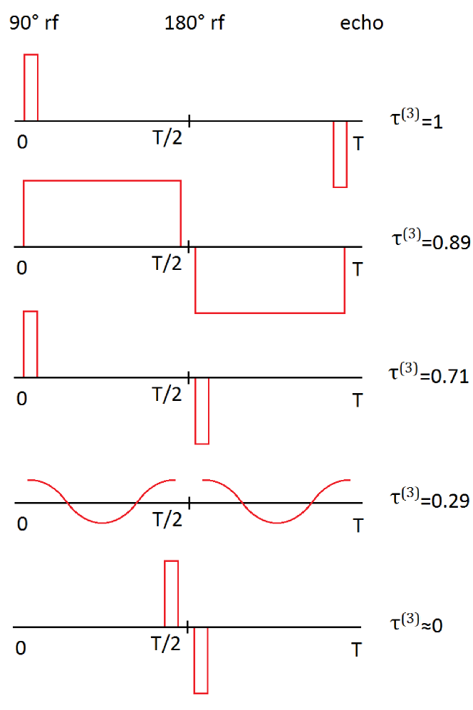
We consider spin-carrying molecules diffusing with scalar intrinsic diffusivity ${\color[rgb]{0,0,0}{D_{0}}}$ in a restricted domain $\Omega$, in the presence of a magnetic field gradient $\bm{g}(t)$, with $t\in[0,T]$. Here, $t=0$ corresponds to the beginning of the gradient sequence after the $90^{\circ}$ radio-frequency (rf) pulse and $t=T$ corresponds to the echo time at which the signal is acquired (see Fig. 1). We presume that there are no magnetic impurities near the domain boundaries, so that the gradient is uniform in the domain. We also assume that the intrinsic diffusivity ${\color[rgb]{0,0,0}{D_{0}}}$ is constant throughout the domain $\Omega$. An extension to multiple isolated compartments with different intrinsic diffusivities and shapes is discussed in Sec. 6.3. We define

$$\bm{q}(t)=\gamma\int_{0}^{t}\bm{g}(t^{\prime})\,\mathrm{d}{t^{\prime}}\;,$$ (2)

where $\gamma$ is the nuclear gyromagnetic ratio, and

$$b=\int_{0}^{T}\lvert\bm{q}(t)\rvert^{2}\,\mathrm{d}{t}\;$$ (3)

is the conventional $b$-value. The gradient profile is supposed to obey the usual refocusing condition

$$\bm{q}(T)={\gamma}\int_{0}^{T}\bm{g}(t)\,\mathrm{d}{t}={\bm{0}}.$$ (4)

From an experimental point of view, this means that $\bm{g}(t)$ is the “effective” gradient which takes into account the effect of refocusing rf-pulses on the spins (for example, the gradient is effectively reversed by a $180^{\circ}$ rf pulse) [38]. This convention allows us to treat spin echo, gradient echo, stimulated echo, and other techniques, with the same formalism.

Figure 1: Illustration of some gradient profiles for spin echo experiments. We stress that these gradient profiles are “effective” in the sense that the gradients are reversed after $T/2$ to include the effect of the $180^{\circ}$ rf pulse. The corresponding values of ${\tau^{(3)}}$ introduced in Sec. 4.1 are given for each profile. Note that ${\tau^{(3)}}=1$ for the narrow pulses-case (first panel), which corresponds to Mitra’s formula (1) with $t=T$.

At small $b$-values (that is, $b{\color[rgb]{0,0,0}{D_{0}}}\ll 1$), the MR signal attenuation $E$ can be written as

$$E\approx\exp(-bD(T))\;,$$ (5)

where $\,\mathrm{d}(T)$ is the effective (or apparent) diffusion coefficient probed by diffusion MR. We generalize the Mitra’s formula (1) as

$$\,\mathrm{d}(T)={\color[rgb]{0,0,0}{D_{0}}}\left(1-\eta\frac{4}{3\sqrt{\pi}}\frac{S}{V}\sqrt{{\color[rgb]{0,0,0}{D_{0}}}T}+O(T)\right)$$ (6)

by introducing the dimensionless prefactor $\eta$ that depends both on the structure of the medium and on the gradient waveform. We stress that dependence on the waveform implies that one cannot, strictly speaking, interpret $\,\mathrm{d}(T)$ as a measure of mean-squared displacement of randomly diffusing molecules, except for the theoretical case of two infinitely narrow gradient pulses.

Using mathematical methods discussed in reviews [39, 8, 40], we derived in Appendix 8 that

$${\eta=\operatorname{Tr}(\mathcal{S}^{(3)}\mathcal{T}^{(3)})}\;,$$ (7)

where $\operatorname{Tr}(\cdot)$ is the trace. Here we introduced the “temporal” matrix $\mathcal{T}^{(3)}$ which is a particular case of the general $\mathcal{T}^{(m)}$ matrices,

$${\mathcal{T}^{(m)}=-\frac{\gamma^{2}T}{2b}\int_{0}^{T}\!\!\int_{0}^{T}\!\bm{g}(t_{1})\otimes\bm{g}(t_{2})\left\lvert\frac{t_{2}-t_{1}}{T}\right\rvert^{m/2}\!\!\,\mathrm{d}{t_{1}}\,\mathrm{d}{t_{2}}\;,}$$ (8)

and the “structural” matrix

$${\mathcal{S}^{(3)}}=\frac{1}{S}\int_{\partial\Omega}\bm{n}\otimes\bm{n}\,\mathrm{d}S\;,$$ (9)

where the integration is performed over the boundary $\partial\Omega$ of the domain $\Omega$ and $\bm{n}$ is the unit outward normal vector to the boundary. In the above formulas, $\otimes$ is the outer product: if ${\bm{a}}$ and ${\bm{b}}$ are vectors, then ${\bm{a}}\otimes{\bm{b}}$ is a matrix with components

$$({\bm{a}}\otimes{\bm{b}})_{ij}=a_{i}b_{j}\;.$$ (10)

Note that $\mathcal{S}^{(3)}$ and $\mathcal{T}^{(m)}$ are tensors in the sense that under a spatial rotation or symmetry described by a matrix $\mathcal{R}$, $\mathcal{S}^{(3)}$ and $\mathcal{T}^{(m)}$ are transformed according to $\mathcal{S}^{(3)}\to\mathcal{R}\mathcal{S}^{(3)}\mathcal{R}^{-1}$ and $\mathcal{T}^{(m)}\to\mathcal{R}\mathcal{T}^{(m)}\mathcal{R}^{-1}$. We note that, with these notations, $\mathcal{T}^{(2)}$ is actually the conventional $b$-matrix renormalized by the $b$-value [19, 20, 21] so that (see Appendix 8 from Eq. (66) to Eq. (68) for a detailed computation)

$$\operatorname{Tr}(\mathcal{T}^{(2)})=1\;.$$ (11)

The correction factor $\eta$ in Eq. (6) is the result of an intricate coupling between the medium structure and the gradient sequence, which is expressed through the simple mathematical relation (7) between $\mathcal{S}^{(3)}$ and $\mathcal{T}^{(3)}$. Note that $\mathcal{S}^{(3)}$ and all $\mathcal{T}^{(m)}$ matrices, in particular $\mathcal{T}^{(3)}$, are dimensionless. As a consequence, $\eta$ is invariant under dilatation of the gradient waveform, dilatation of the time interval $[0,T]$ and dilatation of the domain $\Omega$. The higher-order terms in the asymptotic expansion (6) involve increasing powers of $\sqrt{{\color[rgb]{0,0,0}{D_{0}}}T}$ associated with the temporal matrices $\mathcal{T}^{(m)}$ with increasing integer $m$. These matrices are coupled to structural matrices $\mathcal{S}^{(m)}$ (such as in Eq. (7)) that characterize the medium structure and properties such as curvature, permeability or surface relaxation. However, these properties do not affect the first-order term in (6), on which we focus in this paper. As an example, the second-order, ${\color[rgb]{0,0,0}{D_{0}}}T$, term and the associated matrix $\mathcal{S}^{(4)}$ are discussed in Sec. 6.1.

Mitra’s formula (1) was derived for PGSE experiments with (infinitely) short gradient pulses, where $t=\Delta$ is the inter-pulse time. We emphasize that for general gradient profiles, $\Delta$ is not defined anymore, and we use instead the echo time $T$ in our generalized formula (6). If we compare the two formulas by setting $t=T$ (which corresponds to the profile shown on the first panel in Fig. 1), we see that Mitra’s formula corresponds to the simple expression

$$\eta_{\rm Mitra}=1/d\;.$$ (12)

Below we generalize this relation to arbitrary medium structures (Sec. 3) and gradient profiles (Sec. 4).

3 Dependence on the structure

3.1 Simple shapes

For any bounded domain $\Omega$, the matrix $\mathcal{S}^{(3)}$ is symmetric, positive-definite, and one has $\operatorname{Tr}(\mathcal{S}^{(3)})=1$. For example, if $\Omega$ is a sphere, one gets $\mathcal{S}^{(3)}_{\text{sphere}}=\mathcal{I}/3$, which is invariant under any spatial rotations of the medium, as expected. Throughout the article, we call such matrices, that are proportional to the $3\times 3$ unit matrix $\mathcal{I}$, “isotropic”. However, the same result holds if $\Omega$ is a cube, i.e. the cube is also qualified as isotropic by the $\mathcal{S}^{(3)}$ matrix. Clearly, the matrix $\mathcal{S}^{(3)}$ does not uniquely characterize the shape of $\Omega$.

Let us now consider the example of a rectangular parallelepiped. We choose its sides along the axes $(\bm{e}_{x},\bm{e}_{y},\bm{e}_{z})$ and denote their lengths by $a$, $b$, $c$. Then the normal vector $\bm{n}$ is either $\pm\bm{e}_{x}$, $\pm\bm{e}_{y}$, or $\pm\bm{e}_{z}$ depending on the facet of the parallelepiped, and by integrating over each facet we get

$${\mathcal{S}^{(3)}}=\frac{1}{bc+ca+ab}\begin{bmatrix}bc&0&0\\ 0&ca&0\\ 0&0&ab\end{bmatrix}\;.$$ (13)

This simple example shows that, by varying $a$, $b$, $c$, and applying rotations, the matrix $\mathcal{S}^{(3)}$ can be any symmetric positive-definite matrix with unit trace.

In the limit when one side of the parallelepiped (say, $c$) tends to infinity (or is much bigger than the other two), the rectangular parallelepiped transforms into a cylindrical domain with a rectangular cross-section and the ${\mathcal{S}^{(3)}}$ matrix becomes

$${\mathcal{S}^{(3)}}=\frac{1}{a+b}\begin{bmatrix}b&0&0\\ 0&a&0\\ 0&0&0\end{bmatrix}\;.$$ (14)

Note that in the special case $a=b$ (cylindrical domain with square cross-section), one obtains the same result as for a circular cylinder of axis $\bm{e}_{z}$: ${\mathcal{S}^{(3)}_{\text{cyl}}}=(\mathcal{I}-\bm{e}_{z}\otimes\bm{e}_{z})/2$. In the opposite limit where $a$ and $b$ are much bigger than $c$, the parallelepiped transforms into a slab perpendicular to $\bm{e}_{z}$ and the ${\mathcal{S}^{(3)}}$ matrix becomes ${\mathcal{S}^{(3)}_{\text{slab}}}=\bm{e}_{z}\otimes\bm{e}_{z}$.

One recognizes in the previous examples the factor $1/d$ of Mitra’s formula (1): $1/3$ for a sphere, $1/2$ for a circular cylinder, and $1$ for a slab. However, even in these basic cases, the factor $\eta$ remains affected by the gradient waveform, as discussed in Sec. 4. In Appendix 9, we provide additional computations of $\mathcal{S}^{(3)}$ for slightly non-spherical domains (perturbative computation) and for spheroids (exact computation). Such domains may be more accurate models of anisotropic pores in pathological tissues such as prostate tumor [41] than cylinders.

3.2 The effect of orientation dispersion

Now we consider a random medium consisting of infinite circular cylinders with random orientations and random radii. Cylinders are archetypical anisotropic domains and we choose them to illustrate in an explicit way the effect of orientation dispersion of the domains. They can also serve as a model for alveolary ducts in lungs [42] or muscle fibers [43, 44, 45]. For the sake of simplicity, we assume the radius of each cylinder to be independent from its orientation. Equations (5) and (6) describe the signal on the mesoscopic scale (one cylinder). Within the scope of small $b$-values ($b{\color[rgb]{0,0,0}{D_{0}}}\ll 1$), the macroscopic signal formed by many cylinders is:

$$E\approx\left\langle\exp(-bD(T))\right\rangle\approx\exp(-b\langle\,\mathrm{d}(T)\rangle)\;,$$ (15)

where $\langle\cdots\rangle$ denotes the average over the voxel. Coming back to Eqs. (6) and (7), we see that the average of $\,\mathrm{d}(T)$ is obtained through the average of the ${\mathcal{S}^{(3)}}$ matrices of the cylinders, that we now compute.

From the previous section, the ${\mathcal{S}^{(3)}}$ matrix of a cylinder oriented along any direction $\bm{u}$ (where $\bm{u}$ is a unit vector) is

$${\mathcal{S}^{(3)}_{\text{cyl}}}(\bm{u})=\frac{1}{2}\left(\mathcal{I}-\bm{u}\otimes\bm{u}\right)\;.$$ (16)

Moreover, for one cylinder of radius $R$, one has $S/V=2/R$, thus the voxel-averaged effective diffusion coefficient reads

$$\langle\,\mathrm{d}(T)\rangle={\color[rgb]{0,0,0}{D_{0}}}\left(1-\frac{4\sqrt{{\color[rgb]{0,0,0}{D_{0}}}T}}{3\sqrt{\pi}}\left\langle\!\frac{2}{R}\!\right\rangle\operatorname{Tr}(\langle{\mathcal{S}^{(3)}}\rangle{\mathcal{T}}^{(3)})+O(T)\!\right).$$

The averaged matrix $\langle{\mathcal{S}^{(3)}}\rangle$ depends on the angular distribution of the cylinder orientations. For example, a distribution with a rotation symmetry around the $z$-axis yields

$$\langle{\mathcal{S}^{(3)}}\rangle=\frac{1}{6}\begin{bmatrix}2+{p}&0&0\\ 0&2+{p}&0\\ 0&0&2-2{p}\end{bmatrix}\;,$$ (17)

where ${p}$ is the orientation order parameter (OP) of the medium that is defined as

$${p}=\langle 3\cos^{2}\theta-1\rangle/2=\langle 3u_{z}^{2}-1\rangle/2\;,$$ (18)

where $\theta$ is the random angle between the axis of the cylinder $\bm{u}$ and the symmetry axis $\bm{e}_{z}$. The parameter ${p}$ can take any value from $-1/2$ (for $\theta=\pi/2$, i.e. all the cylinders are in the $x-y$ plane) to $1$ (for $\theta=0$, i.e. all the cylinders are aligned with $\bm{e}_{z}$). The special value ${p}=0$ corresponds to an isotropic matrix ${\mathcal{S}^{(3)}}=\mathcal{I}/3$ and can be obtained, for example, with a uniform distribution [23, 24, 25].

The orientation order parameter has direct analogies with other diffusion models describing the water diffusion in strongly anisotropic medium. For instance, if randomly oriented fibers obey a Watson distribution of parameter $\kappa$ [46], then one can compute [47]

$${p}=\frac{3}{2\sqrt{\pi\kappa}\,e^{-\kappa}\,\operatorname{erfi}(\sqrt{\kappa})}-\frac{3}{4\kappa}-\frac{1}{2}\;,$$ (19)

where $\operatorname{erfi}$ is the imaginary error function. In the limits of $\kappa$ going to $-\infty$, $0$, and $+\infty$, we obtain ${p}=-1/2$, $0$, and $1$, respectively.

An important consequence of the above computations is that experiments at short diffusion times and small-amplitude gradients are unable to distinguish the mesoscopic anisotropy (the anisotropy of each cylinder) inside a macroscopically isotropic medium (uniform distribution of the cylinders). Therefore, regimes with longer diffusion times or higher gradients are needed for extracting mesoscopic diffusion information [23, 24, 48, 49].

4 Dependence on the gradient waveform

In this section we investigate the dependence of the correction factor $\eta$ (and of higher-order terms) on the gradient waveform captured via the ${\mathcal{T}}^{(m)}$ matrices. We begin with the simpler case, the so-called linear gradient encoding, where the gradient $\bm{g}(t)$ has a fixed direction and each ${\mathcal{T}}^{(m)}$ matrix is reduced to a scalar. We show that significant deviations from the classical formula (1) arise depending on the chosen waveform.

Next, in Sec. 4.2, we study how the correction factor is affected in the most general case when both gradient amplitude and direction are time dependent. In particular, we show that recently invented spherical encoding sequences [34, 35] do not provide the full mixing effect in the sense that $\eta$ still depends on the orientation of the (anisotropic) medium. In order to resolve this problem we describe in Sec. 4.3 a simple and robust algorithm to design diffusion gradient profiles with desired features and constraints.

4.1 Linear encoding

If we set $\bm{g}(t)=g(t)\bm{e}$, with a constant unit vector $\bm{e}$, the ${\mathcal{T}}^{(m)}$ matrices become

$${\mathcal{T}}^{(m)}=\tau^{(m)}\,\bm{e}\otimes\bm{e}\;,$$ (20)

with the scalar

$${\tau^{(m)}=-\frac{\gamma^{2}T}{2b}\int_{0}^{T}\int_{0}^{T}g(t_{1})g(t_{2})\,\left\lvert\frac{t_{2}-t_{1}}{T}\right\rvert^{m/2}\,\mathrm{d}{t_{1}}\,\mathrm{d}{t_{2}}\;.}$$ (21)

The correction factor $\eta$ becomes

$${\eta={\tau^{(3)}}\left(\bm{e}^{\dagger}{\mathcal{S}^{(3)}}\bm{e}\right)\;,}$$ (22)

where $\bm{e}^{\dagger}$ denotes the transpose of $\bm{e}$. By keeping the same profile $g(t)$ and only changing the direction of the applied gradient $\bm{e}$, the factor ${\tau^{(3)}}$ is unchanged and the factor $(\bm{e}^{\dagger}{\mathcal{S}^{(3)}}\bm{e})$ allows one to probe the whole ${\mathcal{S}^{(3)}}$ matrix, and thus microstructural information on the domain. For this purpose, one can transpose standard diffusion tensor imaging reconstruction techniques [19] to our case: by choosing multiple non-coplanar directions for $\bm{e}$, one obtains a system of linear equations on the coefficients of ${\mathcal{S}^{(3)}}$ that can be solved numerically. Bearing in mind that ${\mathcal{S}^{(3)}}$ is symmetric positive-definite matrix with trace one, one needs at least $6$ diffusion directions to estimate $5$ independent coefficients of the ${\mathcal{S}^{(3)}}$ matrix and the $S/V$ ratio.

For a ${\mathcal{S}^{(3)}}$ matrix such as the one of a parallelepiped in Eq. (13), the factor $\eta$ takes different values depending on the gradient direction $\bm{e}$. Note that the extremal values of $(\bm{e}^{\dagger}\mathcal{S}^{(3)}\bm{e})$ are given by the minimal and maximal eigenvalue of $\mathcal{S}^{(3)}$. In other words, the relative difference between the extremal eigenvalues of $\mathcal{S}^{(3)}$ indicates the magnitude of the induced error on the estimation of $S/V$. For instance, if one applies the gradient in a direction perpendicular to the smallest facets of parallelepiped, one probes the $S/V$ ratio of these facets, not of the whole structure (see Eq. (13)). Although this example is specific, the conclusion is general: the mesoscopic anisotropy of a confining domain, captured via the matrix ${\mathcal{S}^{(3)}}$, can significantly bias the estimation of the surface-to-volume ratio. This circumstance was ignored in some former studies with application of the classical Mitra’s formula, which is only valid for isotropic domains. While spherical encoding scheme aims to resolve this issue by mixing contributions from different directions, we will see in Sec. 4.2 that this mixing is not perfect for formerly proposed spherical encoding sequences.

In the remaining part of this subsection, we consider the particular case of isotropic (e.g., spherical) domains with ${\mathcal{S}^{(3)}}=\mathcal{I}/3$ so that the structural aspect is fully decoupled from the temporal one. In this case, Eq. (7) yields

$$\eta=\frac{{\tau^{(3)}}}{3}\;,$$ (23)

and we can focus on the temporal aspect (gradient waveform) captured via the factor ${\tau^{(3)}}$. Note that the original Mitra’s formula corresponds to $\tau^{(3)}=1$ (see Eq. (12)).

Figure 1 shows several examples of temporal profiles and the corresponding values of ${\tau^{(3)}}$. The maximum attainable value of ${\tau^{(3)}}$ is slightly over $1$ (around $1.006$), see Appendix 10 for more details. Counter-intuitively, the maximal value of ${\tau^{(3)}}$ is not $1$ while the profile with infinitely narrow pulses does not provide its maximum. The infimum of $\tau^{(3)}$ is $0$; in fact, one can achieve very small values of ${\tau^{(3)}}$ by using very fast oscillating gradients. Indeed, for sinusoidal gradient waveforms of angular frequency $\omega$, one has ${\tau^{(3)}}\sim\omega^{-1/2}$, in the limit $\omega T\gg 1$ (see Appendix 10 and Refs. [16, 17]).

This finding has an important practical consequence: if one ignores the factor ${\tau^{(3)}}$ and uses the original Mitra’s formula (for which ${\tau^{(3)}}=1$), one can significantly underestimate the surface-to-volume ratio (by a factor $1/{\tau^{(3)}}$) and, thus, overestimate the typical size of compartments.

4.2 Isotropy and spherical encoding

Microscopic anisotropy is usually modeled via a non-isotropic diffusion tensor $\mathcal{D}$, and the expression (5) for the diffusion signal becomes

$$E{\approx}\exp\left(-b\operatorname{Tr}\left(\mathcal{T}^{(2)}\mathcal{D}\right)\right)\;.$$ (24)

Typical spherical encoding sequences [30, 27, 31, 32, 33, 34, 35] aim to average out the microscopic anisotropy of the medium by applying an encoding gradient with time-changing direction. Mathematically, the goal is to obtain an isotropic ${\mathcal{T}}^{(2)}$ matrix, ${\mathcal{T}^{(2)}=\mathcal{I}/3}$, so that the signal in Eq. (24) depends only on the trace $\operatorname{Tr}(\mathcal{D})$ and thus yields the same result for any orientation of the medium. We recall that throughout the paper, we call a matrix isotropic if it is proportional to the unit matrix $\mathcal{I}$ (in other words, its eigenvalues are equal to each other).

Mesoscopic anisotropy manifests itself in the ${\mathcal{S}^{(3)}}$ matrix of individual compartments, as we explained in Sec. 3. Thus, from Eq. (6) we can deduce that mesoscopic anisotropy is averaged out (at the order $\sqrt{{\color[rgb]{0,0,0}{D_{0}}}T}$) by the gradient sequence only if ${\mathcal{T}}^{(3)}$ is isotropic. In this case, the factor $\eta$ does not depend on the orientation of the mesoscopically anisotropic medium nor on its actual shape, and one can estimate precisely the surface-to-volume ratio of the medium. Moreover, from Eq. (7) we see that in this case, $\eta$ can be read directly from the expression of ${\mathcal{T}}^{(3)}$:

$${\mathcal{T}}^{(3)}_{\text{iso}}=\eta\,\mathcal{I}\;.$$ (25)

Similarly, the isotropy condition for the matrices ${\mathcal{T}}^{(4)},{\mathcal{T}}^{(5)},\ldots$ would be needed if the higher-order terms of expansion (6) were considered.

Hence, the natural question arises: “Do the former spherical encoding sequences that were designed to get an isotropic ${\mathcal{T}}^{(2)}$ (or $b$) matrix [25], produce isotropic ${\mathcal{T}}^{(m)}$ matrices (or at least ${\mathcal{T}}^{(3)}$)?”. For instance, for the q-Space Magic-Angle-Spinning (q-MAS) sequence [34, 35] we obtain

$${\mathcal{T}}^{(3)}=\begin{bmatrix}0.14&0&0\\ 0&0.28&0.10\\ 0&0.10&0.17\end{bmatrix}\;.$$ (26)

This matrix has eigenvalues $0.11,0.14,0.33$ and is thus not isotropic. Similarly, a triple diffusion encoding (TDE) sequence [30] (where three identical PGSE sequences are applied along three orthogonal direction in space) yields

$${\mathcal{T}}^{(3)}=\begin{bmatrix}0.19&0.08&0.05\\ 0.08&0.19&0.08\\ 0.05&0.08&0.19\end{bmatrix}\;,$$ (27)

with eigenvalues $0.10,0.14,0.34$. Note that, although the diagonal elements of the matrix are identical, it is not isotropic because of the off-diagonal elements. The above matrix corresponds to a TDE sequence where each PGSE sequence is made of infinitely narrow pulses with spacing $\Delta=T/3$. One could also consider the FAMEDcos sequence [50], for which we get

$${\mathcal{T}}^{(3)}=\begin{bmatrix}0.13&0&0.012\\ 0&0.11&0\\ 0.012&0&0.10\end{bmatrix}\;,$$ (28)

which is also not isotropic (with eigenvalues: $0.09,0.11,0.13$). All spherical encoding schemes that we could find in the literature produce anisotropic ${\mathcal{T}}^{(3)}$ matrices.

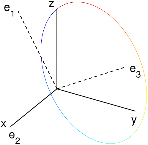
In order to illustrate the errors induced by such sequences in the estimation of the surface-to-volume ratio, let us apply the q-MAS sequence for the case of an infinite circular cylinder. We denote by $(\bm{e}_{1},\bm{e}_{2},\bm{e}_{3})$ the orthogonal basis of eigenvectors and by $(\lambda_{1},\lambda_{2},\lambda_{3})=(0.11,0.14,0.33)$ the corresponding eigenvalues of the ${\mathcal{T}}^{(3)}$ matrix in Eq. (26) (see Fig. 2 for the orientation of these axes with respect to the q-space plot of the sequence). If the cylinder is oriented along $\bm{e}_{3}$, one obtains $\eta=(\lambda_{1}+\lambda_{2})/2=0.13$. However, if the cylinder is oriented along $\bm{e}_{1}$, then $\eta=(\lambda_{2}+\lambda_{3})/2=0.24$, which is nearly twice as large. In other words, the estimated $S/V$ ratio is twice as large in the second situation than in the first one. This artifact is a direct consequence of the differences between the eigenvalues of the ${\mathcal{T}}^{(3)}$ matrix, i.e. its anisotropy.

Figure 2: Plot of $\bm{q}(t)$ for the q-MAS sequence. The color encoding of the trajectory represents time, from $t=0$ (blue) to $t=T$ (red). The additional axes are directed along the eigenvectors ($\bm{e}_{1},\bm{e}_{2},\bm{e}_{3})$ of the $\mathcal{T}^{(3)}$ matrix (26) of the sequence.

4.3 How to obtain isotropic matrices?

The question in the subsection title can be restated in an algebraic language: how to find three functions $g_{x}(t),g_{y}(t),g_{z}(t)$ with zero mean (see Eq. (4)) that are mutually “orthogonal” and have the same “norm” for a given set of symmetric bilinear forms ${\color[rgb]{0,0,0}{\varphi}}_{m},m=2,3,\ldots$, with

$${{\color[rgb]{0,0,0}{\varphi}}_{m}(f_{1},f_{2})=-\frac{\gamma^{2}T}{2b}\!\!\int_{0}^{T}\!\!\!\int_{0}^{T}\!\!f_{1}(t_{1})f_{2}(t_{2})\left\lvert\frac{t_{1}-t_{2}}{T}\right\rvert^{m/2}\!\!\,\mathrm{d}{t_{1}}\,\mathrm{d}{t_{2}}\;.}$$ (29)

Since the space of functions with zero mean is infinite-dimensional, we can be confident in finding such three functions. However, Eq. (29) involves a non-integer power of time that prevents us from getting analytical solution for this problem. Thus, we design a simple algorithm for generating the gradient sequences that satisfy these conditions.

The idea is to choose a family of functions $(f_{1},f_{2},\ldots,f_{k})$ (for example, sines or polynomials, possibly with phase jumps at $T/2$) and to search for $g_{x}(t),g_{y}(t),g_{z}(t)$ as linear combinations of the basis functions. This is a generalization of the classical sine and cosine decomposition which was already used in the context of waveform optimization [35]. Mathematically, this means that

$$\begin{pmatrix}g_{x}(t)\\ g_{y}(t)\\ g_{z}(t)\end{pmatrix}=X\begin{pmatrix}f_{1}(t)\\ f_{2}(t)\\ \vdots\\ f_{k}(t)\end{pmatrix}\;,$$ (30)

where $X$ is a $3\times k$ matrix of coefficients to be found. Now we define the $k\times k$ matrices $\Phi^{(m)}$ by

$${\Phi}^{(m)}_{i,j}={\color[rgb]{0,0,0}{\varphi}}_{m}(f_{i},f_{j})\;,\quad m=2,3,\ldots$$ (31)

In this way, one can compute directly the ${\mathcal{T}}^{(m)}$ matrices according to

$${\mathcal{T}}^{(m)}=X{\Phi}^{(m)}X^{\dagger}\;.$$ (32)

The problem is then reduced to an optimization problem for the matrix $X$, which can be easily done numerically. In other words, one searches for a matrix $X$ that ensures the isotropy of the matrix ${\mathcal{T}}^{(3)}$. In the same way, one can generate a sequence with both isotropic $\mathcal{T}^{(2)}$ and $\mathcal{T}^{(3)}$ matrices, or any other combination of isotropic $\mathcal{T}^{(m)}$ matrices. At the same time, we prove in Appendix 11 that there is no gradient sequence that produces isotropic $\mathcal{T}^{(m)}$ matrices simultaneously for all integers $m\geq 2$.

The optimization algorithm can include various additional constraints. On one hand, one has a freedom to choose an appropriate family $(f_{1},f_{2},\ldots,f_{k})$, for example, to ensure smoothness of the resulting gradient profile. Similarly, the refocusing condition can be achieved by choosing zero-mean functions. On the other hand, it is also possible to add some constraints as a part of the optimization problem. This is especially easy if the constraints can be expressed as linear or bilinear forms of the gradient profile $\bm{g}(t)$. For instance, each ${\mathcal{T}}^{(m)}$ matrix in (8) is a bilinear form of the gradient profile allowing one to express them as the simple matrix multiplication (32). Another example of additional conditions consists in imposing zeros to the designed gradient profiles. Indeed, for practical reasons, it is often easier to manipulate with the gradients that satisfy to

$$\bm{g}(0)=\bm{g}(T/2)=\bm{g}(T)={\bm{0}}\;.$$ (33)

This is a linear condition on the gradient profile. If one denotes by $\mathcal{V}$ the $k\times 3$ matrix

$$\mathcal{V}=\begin{bmatrix}f_{1}(0)&f_{1}(T/2)&f_{1}(T)\\ f_{2}(0)&f_{2}(T/2)&f_{2}(T)\\ \vdots&\vdots&\vdots\\ f_{k}(0)&f_{k}(T/2)&f_{k}(T)\end{bmatrix}\;,$$ (34)

then Eq. (33) becomes

$$X\mathcal{V}=\begin{bmatrix}0&0&0\\ 0&0&0\\ 0&0&0\end{bmatrix}\;.$$ (35)

In the following, we impose the above condition to produce our gradient waveforms.

It is worth to note that one can also generate flow-compensated gradients, or more generally, motion artifacts suppression techniques, by imposing linear conditions on the gradient profile

$$\int_{0}^{T}t^{p}\bm{g}(t)\,\mathrm{d}{t}={\bm{0}}\;,\quad p=1,2,\ldots,{P}\;,$$ (36)

where $p=1$ corresponds to the flow compensation, and higher values of $p$ account for acceleration, pulsatility, etc. [51, 52]. This condition can be rewritten in the matrix form $X\mathcal{M}=0$, where the $k\times{P}$ matrix $\mathcal{M}$ is defined by

$$\mathcal{M}_{i,p}=\int_{0}^{T}t^{p}f_{i}(t)\,\mathrm{d}{t}\;,\quad p=1,2,\ldots,{P}\;.$$ (37)

Another type of optimizaton constraints can be based on hardware limitations such as a need to minimize heat generation during the sequence execution which amounts to minimizing the following quantity

$$\langle\bm{g},\bm{g}\rangle=\int_{0}^{T}\lvert\bm{g}(t)\rvert^{2}\,\mathrm{d}{t}\;,$$ (38)

which is a bilinear form of the gradient profile. Similar to representation (32) for ${\mathcal{T}}^{(3)}$, one can define a matrix $\mathcal{H}_{i,j}=\langle f_{i},f_{j}\rangle$ to write Eq. (38) as $\langle\bm{g},\bm{g}\rangle=\operatorname{Tr}\left(X\mathcal{H}X^{T}\right)$, and then to include it into the optimization procedure.

The previous examples showed how linear and bilinear forms of the gradient profile can be simply expressed in terms of the weights matrix $X$, which allows one to perform very fast computations. The matrix corresponding to each condition (for example, ${\Phi^{(3)}}$, $\mathcal{V}$, $\mathcal{H}$) has to be computed only once, then optimization is reduced to matrix multiplications. The size of the matrices involved in the computations is defined by the size of the chosen set of functions $(f_{1},\ldots,f_{k})$. Note that the set size is independent of the numerical sampling of the time interval $[0,T]$ that controls accuracy of the computations.

Some properties of the designed gradients do not fall into the category of aforementioned linear or bilinear forms, e.g., “max” amplitude-function (i.e., one cannot impose the maximal gradient constraint in this way). They can be included in the optimization, however one cannot apply the previous techniques in order to speed up the computation.

We have to emphasize that the “optimal” solution is not unique and it depends on the choice of the set $f_{1},\ldots,f_{k}$. Moreover, if the set is sufficiently large and the number of degrees of freedom is greater than the number of constraints, then the algorithm will likely yield different solutions depending on the initial choice of $X$ for an iterative solver. This property can be advantageous in practice, as one can design many optimal solutions. The described optimization algorithm was implemented in Matlab (The MathWorks, Natick, MA USA) and is available upon request. It concatenates all the chosen constraints in a single matrix-valued function $f(X)$ of the weight matrix $X$, in such a way that the constraints are expressed by the condition $f(X)=0$. This equation is then solved numerically with the Levenberg-Marquardt algorithm.

Figure 3: Two examples of gradient waveforms that produce an isotropic ${\mathcal{T}}^{(3)}$ matrix and that satisfy Eq. (33). Note that the gradients are “effective” gradients in the sense that we reversed them after the $180^{\circ}$ rf pulse at $T/2$. The bottom figure shows the corresponding $\bm{q}(t)$. The color encoding of the trajectory represents time, from $t=0$ (blue) to $t=T$ (red). (left) the profiles are combination of $9$ piecewise sine and cosine functions with frequencies up to $6/T$, and in addition they satisfy isotropy of $\mathcal{T}^{(2)}$; (right) the profiles are piecewise polynomials of order $5$, and they satisfy ${\mathcal{T}}^{(4)}=0$.

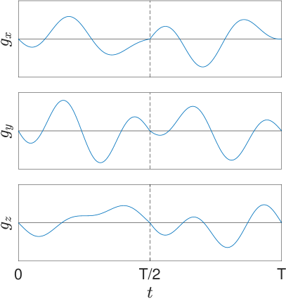
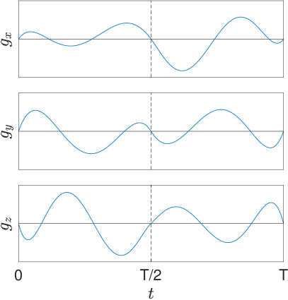
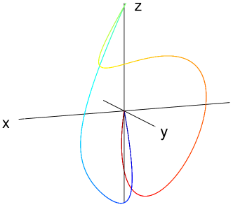
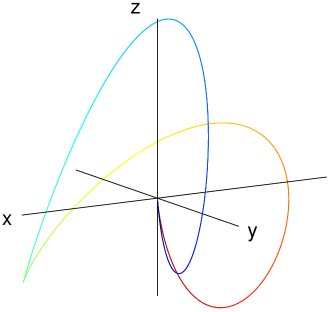
Figure 3 shows two examples of gradient waveforms that produce an isotropic ${\mathcal{T}}^{(3)}$ matrix. These profiles were obtained from two sets with $k=9$ functions. The first set was composed of $\cos(\pi jt/T)$ with $j=1,\ldots,5$; $\sin(\pi jt/T)$ with $j=2,4,6$; and $\varepsilon(t)\sin(4\pi t/T)$ where $\epsilon(t)$ is a piecewise constant function that is equal to $1$ on $[0,T/2]$ and $-1$ on $(T/2,T]$. We also imposed the condition of isotropy of $\mathcal{T}^{(2)}$. The second set was composed of a mixture of monomials, symmetrized odd monomials and antisymmetrized even monomials, with zero mean: $(t-T/2)$, $(t-T/2)^{2}-T^{2}/12$, $(t-T/2)\lvert t-T/2\rvert$, $(t-T/2)^{3}$, $\lvert t-T/2\rvert^{3}-T^{3}/32$, $(t-T/2)^{4}-T^{4}/80$, $(t-T/2)^{3}\lvert t-T/2\rvert$, $(t-T/2)^{5}$, $\lvert t-T/2\rvert^{5}-T^{5}/192$. In this case, we imposed the condition of vanishing $\mathcal{T}^{(4)}$. Although the combination of symmetric and antisymmetric functions helped us to increase the number of basis functions while keeping low degree monomials or slowly oscillating sines, one could alternatively use just monomials, polynomials, or other basis functions as well. Note that there is no need to impose the orthogonality of the basis functions $f_{1},\ldots f_{k}$.

Figure 4: Effective diffusion coefficient $\,\mathrm{d}(T)/{\color[rgb]{0,0,0}{D_{0}}}$ plotted against $\frac{S}{V}\sqrt{{\color[rgb]{0,0,0}{D_{0}}}T}$ inside a prolate spheroid with semi-axes $10\,\mu{\rm m}$ and $5\,\mu{\rm m}$ for two gradient sequences and two orientations of the spheroid. The intrinsic diffusivity is ${\color[rgb]{0,0,0}{D_{0}}}=1\,\mu{\rm m^{2}/ms}$. The simulation results are shown as symbols and the generalized Mitra formula is plotted as line. (left) q-MAS sequence: different orientations of the domain produce different $\,\mathrm{d}(T)$ curves. (right) Optimized sequence with isotropic $\mathcal{T}^{(3)}$ and zero $\mathcal{T}^{(4)}$: the $\,\mathrm{d}(T)$ curves are the same for different orientations of the domain because of the condition on $\mathcal{T}^{(3)}$. Moreover, the condition on $\mathcal{T}^{(4)}$ extends the range of validity of the theoretical formula to about $20\,{\rm ms}$.

Let us consider the waveform obtained in the left panel of Fig. 3. The condition of isotropy for both matrices ${\mathcal{T}}^{(2)}$ and ${\mathcal{T}}^{(3)}$ yields $5+5$ equations on the components of matrix $X$. Besides of matrices ${\mathcal{T}}^{(2,3)}$, condition (33) adds another $9$ equations on the components of $X$. Moreover, we imposed the $b$-value so that the algorithm satisfied $20$ conditions with $3k=27$ degrees of freedom.

The gradient waveform corresponds to $\eta\approx 0.1$ and the dimensionless $b$-value is $b/(\gamma^{2}G_{\rm max}^{2}T^{3})\approx 0.006$ (with $G_{\rm max}$ being the maximum gradient amplitude). Hence the $b$-value is about three times smaller than what one can achieve with only the condition on the isotropy of ${\mathcal{T}}^{(2)}$ [35]. Instead of only constraining ${\mathcal{T}}^{(3)}$ to be isotropic, one can in addition impose a precise value of $\eta$ by using Eq. (25). However we observed that the algorithm could not produce gradient waveforms with arbitrary values of $\eta$: there were bounds for $\eta$-values outside of which the optimization process did not converge. This behavior was expected, because even in the linear encoding case, there were mathematical limitations for the parameter $\eta$ (see Sec. 4.1 and Appendix 10). These bounds can be extended by adding more basis functions (i.e., by increasing the size $k$ of their set). Another way to extend the bounds is to reduce the number of constraints, for example, by dropping out the condition of isotropic ${\mathcal{T}}^{(2)}$ matrix and only keeping the condition on ${\mathcal{T}}^{(3)}$. Indeed, the isotropy of $\mathcal{T}^{(2)}$ is only required in the case of a microscopically anisotropic medium, which we did not assume here (see Appendix 6.2).

Interestingly, the ${\mathcal{T}}^{(4)}$ matrix presents a special case: integrating by parts in Eq. (8) one can show that

$${\mathcal{T}}^{(4)}=\left(\int_{0}^{T}\bm{q}(t)\,\mathrm{d}{t}\right)\otimes\left(\int_{0}^{T}\bm{q}(t)\,\mathrm{d}{t}\right)\;.$$ (39)

This implies that the matrix has rank one, so it cannot be proportional to the unit matrix unless it is null, that occurs under the simple condition

$$\int_{0}^{T}\bm{q}(t)\,\mathrm{d}t=\mathbf{0}\;.$$ (40)

This condition can be easily included in our optimization algorithm. This is the case for the designed profile shown on the right panel in Fig. 3. As a consequence, the corresponding term (of the order of ${\color[rgb]{0,0,0}{D_{0}}}T$) vanishes in the expansion (6). Note that in the presence of permeation or surface relaxation, an additional term of the order of ${\color[rgb]{0,0,0}{D_{0}}}T$ would be present in the expansion (6) and would not necessarily vanish if ${\mathcal{T}}^{(4)}=0$. We do not consider these effects in the paper.

The property of vanishing ${\color[rgb]{0,0,0}{D_{0}}}T$-order term is well-known for cosine-based waveforms with an integer number of periods [53], and, indeed, such functions automatically satisfy to Eq. (40). However, this property is not exclusive to cosine functions (for example, the right panel of Fig. 3 was obtained with polynomial functions). It is also easy to show that Eq. (40) is equivalent to condition (36) for $p=1$. In other words, flow-compensated gradient profiles automatically cancel the ${\color[rgb]{0,0,0}{D_{0}}}T$-order correction term in the generalized Mitra’s expansion, as it was pointed out earlier in [52].

5 Monte Carlo simulations

We performed Monte Carlo simulations to illustrate our theoretical results. The confining domain $\Omega$ is a prolate spheroid with major and minor semi-axes equal to $10\,\mu{\rm m}$ and $5\,\mu{\rm m}$. The intrinsic diffusion coefficient ${\color[rgb]{0,0,0}{D_{0}}}$ is $1\,\mu{\rm m^{2}/ms}$ and the echo time $T$ ranges from $0$ to $25\,{\rm ms}$. Reflecting conditions were implemented at the boundary of the domain and the interval $[0,T]$ was divided into $200$ time steps of equal duration. For each value of $T$, we generated about $5\cdot 10^{6}$ trajectories, applied the gradient sequence and computed the effective diffusion coefficient $\,\mathrm{d}(T)$ from the second moment of the random dephasing $\phi$ of the particles: $\,\mathrm{d}(T)=\langle\phi^{2}\rangle/(2b)$. In order to generate random initial positions for the particles inside the spheroid, we generated random positions inside a larger parallelepiped then discarded the particles that were outside the spheroid. We checked that the randomness in the effective number of particles was very small relatively to the number of particles (less than $0.1\%$).

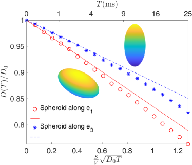
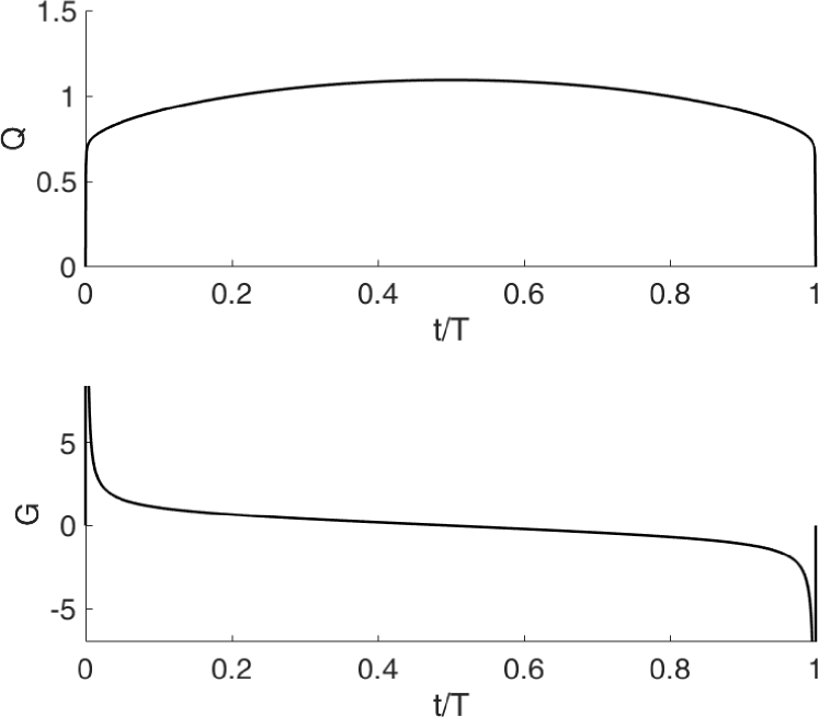
We chose two different gradient sequences: the q-MAS sequence [34, 35] and an optimized sequence with isotropic $\mathcal{T}^{(3)}$ and zero $\mathcal{T}^{(4)}$ such as the one in the right panel of Fig. 3. Note that we could have replaced the q-MAS sequence by any other 3D gradient sequence from the present literature, such as triple diffusion encoding (TDE) [30]. For each sequence, we chose two different orientations of the spheroid that yielded maximal and minimal value of $\eta$. This can be done by finding numerically the eigenvectors $(\bm{e}_{1},\bm{e}_{2},\bm{e}_{3})$ of the $\mathcal{T}^{(3)}$ matrix (sorted by increasing eigenvalue) and then orienting the spheroid along $\bm{e}_{1}$ and $\bm{e}_{3}$, respectively (see for example Fig. 2). The $\,\mathrm{d}(T)$ curves are presented on Fig. 4. The $\mathcal{S}^{(3)}$ matrix of a spheroid can be computed exactly (see Appendix 9) and we plotted simulation results alongside analytical results.

The comparison between the two graphs reveals several important features. First, as we argued in the previous section, the q-MAS sequence is not isotropic with respect to mesoscopic anisotropy studied with short-time experiments. Different orientations of the spheroid yield different values of $\eta$ ($0.15$ and $0.22$, respectively) and thus, different $\,\mathrm{d}(T)$ curves. In turn, if one does not know a priori what is the orientation of the spheroid, then it is impossible to recover its $S/V$ ratio from one $\,\mathrm{d}(T)$ curve, as $\eta$ depends on this orientation. In this case, one may estimate $\eta$ from its average over different orientations of the domain: $\eta\approx\operatorname{Tr}\left(\mathcal{T}^{(3)}\right)/3$. For the q-MAS sequence this would yield $\eta\approx 0.20$.

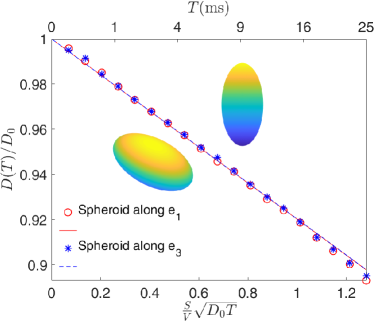
On the other hand, sequences with isotropic $\mathcal{T}^{(3)}$ produce the same coefficient $\eta$ independently of the shape or orientation of the domain. Thus, one obtains the same $\,\mathrm{d}(T)$ curve for the two orientations of the spheroid that allows one to recover its $S/V$ ratio from a single measurement.

Another important point lies in the range of validity of the first-order generalized Mitra formula (6). One can clearly see the effect of zero $\mathcal{T}^{(4)}$ matrix that extends the range of validity from about $5\,{\rm ms}$ to about $20\,{\rm ms}$. This comes at the price of a lower $\eta$ (here, $\eta=0.11$), meaning a slower decay of $\,\mathrm{d}(T)$, which is however compensated by the extension of the range of $T$. Note that this extension of the range of $T$ may also compensate for a smaller $b$-value. In all these cases, the $\eta$ values are significantly different from $1/3$ given by Mitra’s original formula (see Eq. (12)).

6 Extensions

In this section we examine several extensions of our results. First we investigate in more details the next order, ${\color[rgb]{0,0,0}{D_{0}}}T$, term of expansion (6). Then we turn to the case where the medium is microscopically anisotropic, i.e. the diffusivity is a tensor $\mathcal{D}$. Finally we discuss the effects of multiple compartments with different pore shapes and/or intrinsic diffusivities ${\color[rgb]{0,0,0}{D_{0}}}$.

6.1 Order ${\color[rgb]{0,0,0}{D_{0}}}T$ term

From the short-time expansion of heat kernels [54, 55, 56] one can compute the next-order term of $\,\mathrm{d}(T)$ as

$$\frac{\,\mathrm{d}(T)}{{\color[rgb]{0,0,0}{D_{0}}}}=\!1-\eta\frac{4}{3\sqrt{\pi}}\frac{S}{V}\sqrt{{\color[rgb]{0,0,0}{D_{0}}}T}-\eta^{(4)}\frac{C_{0}S}{2V}{\color[rgb]{0,0,0}{D_{0}}}T+O(T^{3/2}),$$ (41)

where $\eta^{(4)}$ is a dimensionless parameter defined as

$$\eta^{(4)}=\operatorname{Tr}\left(\mathcal{S}^{(4)}\mathcal{T}^{(4)}\right)\;.$$ (42)

In the above formula, the structural matrix $\mathcal{S}^{(4)}$ is

$$\mathcal{S}^{(4)}=\frac{1}{C_{0}S}\int_{\partial\Omega}C\,\bm{n}\otimes\bm{n}\,\mathrm{d}{S}\;,$$ (43)

where $C$ is the local mean curvature of the surface, i.e. $C=(R_{1}^{-1}+R_{2}^{-1})/2$, where $R_{1}$ and $R_{2}$ are the local principal radii of curvature of the boundary $\partial\Omega$ of the domain. The integral is normalized by $S$ and by the average curvature of $\partial\Omega$: $C_{0}=(1/S)\int_{\partial\Omega}C\d{S}$. Note that this normalization ensures that the matrix $\mathcal{S}^{(4)}$ has unit trace.

Thus, one can potentially probe the curvature of the boundary of the domain by measuring the ${\color[rgb]{0,0,0}{D_{0}}}T$ correction term in the short-time expansion of $\,\mathrm{d}(T)$. Note that, as we mentioned in Sec. 4.3, the $\mathcal{T}^{(4)}$ matrix has rank one so that one would need at least three measurements (for example, the same linear gradient sequence in three orthogonal directions) in order to average out the anisotropy of $\mathcal{S}^{(4)}$ and recover $C_{0}$. We recall that we ignore permeation and surface relaxation that manifest in the ${\color[rgb]{0,0,0}{D_{0}}}T$ term as well.

6.2 Tensor diffusivity

In this work, we specifically focused on mesoscopic anisotropy and excluded the effect of microscopic anisotropy by choosing a scalar diffusivity ${\color[rgb]{0,0,0}{D_{0}}}$. However, some of our results may be extended to a tensor diffusivity $\mathcal{D}$. Let us assume that the eigenvectors of $\mathcal{D}$ are directed along $\bm{e}_{x}$, $\bm{e}_{y}$, $\bm{e}_{z}$, with $\mathcal{D}_{xx}$, $\mathcal{D}_{yy}$, $\mathcal{D}_{zz}$ being the corresponding eigenvalues. The mean diffusivity is ${\color[rgb]{0,0,0}{D_{0}}}=\operatorname{Tr}(\mathcal{D})/3$. Let us denote by $\mathcal{S}^{(2)}$ the matrix defined by $\mathcal{S}^{(2)}=\mathcal{D}/{\color[rgb]{0,0,0}{D_{0}}}$.

By applying the affine mapping of matrix $\mathcal{L}=\sqrt{\mathcal{S}^{(2)}}^{-1}$, i.e. a spatial dilatation by the factor $\sqrt{{\color[rgb]{0,0,0}{D_{0}}}/\mathcal{D}_{ii}}$ for each direction $i=x,y,z$, one transforms the anisotropic diffusion tensor $\mathcal{D}$ into the isotropic diffusion tensor ${\color[rgb]{0,0,0}{D_{0}}}\mathcal{I}$. The domain and the gradient are also affected by this transformation and we denote by prime the new quantities. For instance, spheres are transformed in ellipsoids by this transformation. As the gradient is also affected by the matrix $\mathcal{L}^{-1}$, one has $\mathcal{T}^{(m)}{}^{\prime}=\mathcal{L}^{-1}\mathcal{T}^{(m)}\mathcal{L}^{-1}$. While the new volume is $V^{\prime}=\det(\mathcal{L})V$, there is no simple formula for the surface $S^{\prime}$ and the $\mathcal{S}^{(3)}{}^{\prime}$ matrix. Applying our results on isotropic diffusivity to this new case, we get for the effective diffusion coefficient in the original system

$$\,\mathrm{d}(T)={\color[rgb]{0,0,0}{D_{0}}}\left(\operatorname{Tr}(\mathcal{S}^{(2)}\mathcal{T}^{(2)})-\eta^{\prime}\frac{4}{3\sqrt{\pi}}\frac{S^{\prime}}{V^{\prime}}\sqrt{{\color[rgb]{0,0,0}{D_{0}}}T}+O(T)\right)\;,$$ (44)

where

$$\eta^{\prime}=\operatorname{Tr}(\mathcal{S}^{(3)}{}^{\prime}\mathcal{T}^{(3)}{}^{\prime})=\operatorname{Tr}(\mathcal{L}^{-1}\mathcal{S}^{(3)}{}^{\prime}\mathcal{L}^{-1}\mathcal{T}^{(3)})\;.$$ (45)

From the above equation we obtain that $\,\mathrm{d}(T)$ does not depend (to the order $\sqrt{{\color[rgb]{0,0,0}{D_{0}}}T}$) on the orientation of the gradient sequence with respect to the medium if $\mathcal{T}^{(2)}$ and $\mathcal{T}^{(3)}$ are isotropic. As we mentioned before, the condition of isotropy of the temporal matrix $\mathcal{T}^{(2)}$ is equivalent to the isotropy of the $b$-matrix that is achieved by spherical encoding techniques [30, 27, 31, 32, 33, 34, 35].

6.3 Multiple compartments

Our results were derived under the assumption of a spatially homogeneous intrinsic diffusivity. Moreover, except in Sec. 3.2 where we investigated the effect of orientation dispersion of the confining pores, we implicitly assumed that all confining pores are identical. Here we present an extension to a medium that is composed of two or more non-communicating (isolated) compartments (for example, intra- and extra-cellular spaces) with different diffusion coefficients and/or different confining pores .

Inside each compartment, the diffusivity is constant and the pore shapes are identical, so that our formula (6) for $\,\mathrm{d}(T)$ is valid, with parameters ${\color[rgb]{0,0,0}{D_{0}}}$, $\eta$, $S/V$ that depend on the compartment. The signal can be computed as a voxel-average of signals from individual compartments, and in the regime of small $b$-values ($b{\color[rgb]{0,0,0}{D_{0}}}\ll 1$), one has, in analogy to Eq. (15),

$$E\approx\langle\exp(-bD(T))\rangle\approx\exp(-b\langle\,\mathrm{d}(T)\rangle)\;,$$ (46)

where the average is weighted by the relative volume of each compartment, and

$$\langle\,\mathrm{d}(T)\rangle=\langle{\color[rgb]{0,0,0}{D_{0}}}\rangle-\frac{4}{3\sqrt{\pi}}\left\langle\eta\frac{S}{V}{\color[rgb]{0,0,0}{D_{0}}}^{3/2}\right\rangle\sqrt{T}+O(T)\;.$$ (47)

We keep this general form of the voxel average which depends on the specific configuration of compartments, pore shapes, diffusivities, etc.

In the above reasoning, the hypothesis of non-communicating compartments is crucial and further modifications would be needed in order to include exchange between compartments when a nucleus can experience different diffusion coefficients during the measurement.

7 Conclusion

We presented a generalization of Mitra’s formula that is applicable to any gradient waveform and any geometrical structure. This generalized formula differs from the classical one by a correction factor in front of $S/V$. In the case of linear encoding schemes, we showed that this factor can significantly affect the estimation of $S/V$ and lead to overestimated size of compartments.

We also discussed in detail the effect of anisotropy of the medium and the use of spherical encoding schemes. In particular, we showed that in order to estimate the surface-to-volume ratio of a mesoscopically anisotropic medium, the gradient should satisfy the isotropy condition (${\mathcal{T}}^{(3)}\propto\mathcal{I}$) that is different from the usual one (${\mathcal{T}}^{(2)}\propto\mathcal{I}$). In particular, typical spherical encoding schemes do not satisfy this new condition. We presented a simple and flexible algorithm that allows fast optimization of gradient waveforms and is well-suited for design of diffusion weighted sequences with specific features such as isotropy of ${\mathcal{T}}^{(3)}$, flow compensation, heat limitation, and others.

The developed extension of Mitra’s formula is expected to have a significant practical impact due to temporal diffusion encoding parametrization [17, 50], in particular, in medical applications [12, 57, 58]. The proposed approach characterizes the underlying microstructure via novel quantitative metrics such as ${\mathcal{S}^{(3)}}$-tensor and more accurate surface-to-volume ratio. The quantitative scalar maps based on those metrics possess a high potential as a novel set of biomarkers and allow one to apply both well-known diffusion tensor formalism and further improvement of diffusion models based on compartmentization. The practical advantages of the developed approach for designing new gradient encoding schemes for in vivo brain imaging on clinical scanners will be demonstrated in a separate publication.

8 Theoretical computations

The signal is proportional to the expectation of the transverse magnetization which has a form of the characteristic function of the random dephasing $\phi$ acquired by diffusing spin-carrying molecules:

$$E={\mathbb{E}}\{e^{{-}i\phi}\},\quad\phi=\gamma\int\limits_{0}^{T}B(\bm{r}(t),t)\,\mathrm{d}{t}\;,$$ (48)

where $T$ is the echo time, $\bm{r}(t)$ is the random trajectory of the nucleus, $\gamma$ is the gyromagnetic ratio, and $\gamma B(\bm{r},t)$ is the Larmor frequency corresponding to the magnetic field. In this work, we consider the most general form of the linear gradient $\bm{g}(t)$:

$$B(\bm{r},t)=\bm{g}(t)\cdot\bm{r}=g_{x}(t)x+g_{y}(t)y+g_{z}(t)z.$$ (49)

In particular, the dephasing can be decomposed as

$$\phi=\phi_{x}+\phi_{y}+\phi_{z},\quad\phi_{i}=\gamma\int\limits_{0}^{T}dt\,g_{i}(t)(\bm{e}_{i}\cdot\bm{r}(t))\quad(i=x,y,z),$$ (50)

where $\bm{e}_{x}$, $\bm{e}_{y}$ and $\bm{e}_{z}$ are the units vectors in three directions, and $(\bm{e}_{i}\cdot\bm{r}(t))$ is the projection of the molecule position at time $t$ onto the direction $\bm{e}_{i}$.

The effective diffusion coefficient is related to the second moment of the dephasing, i.e., we need to evaluate

$${\mathbb{E}}\{\phi^{2}\}=\sum\limits_{i,j=x,y,z}{\mathbb{E}}\{\phi_{i}\phi_{j}\}.$$ (51)

We emphasize that the three components $\phi_{x}$, $\phi_{y}$ and $\phi_{z}$ are independent only for free diffusion, whereas confinement would typically make them correlated. In other words, one cannot a priori ignore the cross terms such as ${\mathbb{E}}\{\phi_{x}\phi_{y}\}$.

In order to compute these terms, we use the following representation [8]:

$${\mathbb{E}}\{\phi_{i} \phi_{j}\}=\gamma^{2}\int_{0}^{T}\!\!\,\mathrm{d}{t_{1}}\int_{t_{1}}^{T}\!\,\mathrm{d}{t_{2}}\int_{\Omega}\!\,\mathrm{d}{\bm{r}_{0}}\int_{\Omega}\!\,\mathrm{d}{\bm{r}_{1}}\int_{\Omega}\!\,\mathrm{d}{\bm{r}_{2}}\int_{\Omega}\!\,\mathrm{d}{\bm{r}_{3}}$$

$$\times\rho(\bm{r}_{0})P_{t_{1}}(\bm{r}_{0},\bm{r}_{1})P_{t_{2}-t_{1}}(\bm{r}_{1},\bm{r}_{2})P_{T-t_{2}}(\bm{r}_{2},\bm{r}_{3})$$

$$\times\left[B_{i}(\bm{r}_{1},t_{1})B_{j}(\bm{r}_{2},t_{2})+B_{j}(\bm{r}_{1},t_{1})B_{i}(\bm{r}_{2},t_{2})\right]$$ (52)

where $P_{t}(\bm{r},\bm{r}^{\prime})$ is the propagator in the domain $\Omega$, and $\rho(\bm{r}_{0})$ is the initial density of particles (the initial magnetization after the $90^{\circ}$ rf pulse). If the boundary is fully reflecting and $\rho(\bm{r}_{0})$ is uniform, then the integrals over $\bm{r}_{0}$ and $\bm{r}_{3}$ yield $1$, so that

$${\mathbb{E}}\{\phi_{i} \phi_{j}\}=\frac{\gamma^{2}}{V}\int_{0}^{T}\!\,\mathrm{d}{t_{1}}\int_{t_{1}}^{T}\!\,\mathrm{d}{t_{2}}\int_{\Omega}\!\,\mathrm{d}{\bm{r}_{1}}\int_{\Omega}\!\,\mathrm{d}{\bm{r}_{2}}P_{t_{2}-t_{1}}(\bm{r}_{1},\bm{r}_{2})$$

$$\times\left[B_{i}(\bm{r}_{1},t_{1})B_{j}(\bm{r}_{2},t_{2})+B_{j}(\bm{r}_{1},t_{1})B_{i}(\bm{r}_{2},t_{2})\right],$$ (53)

where $V$ is the volume of the domain. We get thus

$${\mathbb{E}}\{\phi_{i} \phi_{j}\}=\gamma^{2}\int_{0}^{T}\!\,\mathrm{d}{t_{1}}\,g_{i}(t_{1})\int_{t_{1}}^{T}\!\,\mathrm{d}{t_{2}}\,g_{j}(t_{2})K_{ij}(t_{2}-t_{1})$$

$$+\int_{0}^{T}\!\,\mathrm{d}{t_{1}}\,g_{j}(t_{1})\int_{t_{1}}^{T}\!\,\mathrm{d}{t_{2}}\,g_{i}(t_{2})K_{ji}(t_{2}-t_{1}),$$ (54)

where

$$K_{ij}(t)={\frac{1}{V}}\int_{\Omega}\int_{\Omega}{p}_{i}(\bm{r}_{1})P_{t}(\bm{r}_{1},\bm{r}_{2}){p}_{j}(\bm{r}_{2})\,\mathrm{d}{\bm{r}_{1}}\,\mathrm{d}{\bm{r}_{2}},$$ (55)

with ${p}_{i}(\bm{r})=(\bm{e}_{i}\cdot\bm{r})$. Since $K_{ij}(t)=K_{ji}(t)$ due to the symmetry of the propagator, we can rewrite the moment as

$${\mathbb{E}}\{\phi_{i}\phi_{j}\}=\gamma^{2}\int_{0}^{T}g_{i}(t_{1})\int_{0}^{T}g_{j}(t_{2})K_{ij}(|t_{2}-t_{1}|)\,\mathrm{d}{t_{1}}\,\mathrm{d}{t_{2}}.$$ (56)

We rely on the general short-time expansion for the heat kernels (see [54, 55, 56] and references therein)

$$K_{ij}(t)=\sum\limits_{m\geq 0}c_{m}(p_{i},p_{j})\,({\color[rgb]{0,0,0}{D_{0}}}t)^{m/2},$$ (57)

with

$$c_{0}(f,{h}) =\frac{1}{V}\int_{\Omega}f(\bm{r}){h}(\bm{r})\,\mathrm{d}{\bm{r}}\;,$$ (58a)

$$c_{1}(f,{h}) =0\;,$$ (58b)

$$c_{2}(f,{h}) =-\frac{1}{V}\int_{\Omega}\nabla f(\bm{r})\cdot\nabla{h}(\bm{r})\,\mathrm{d}{\bm{r}}\;,$$ (58c)

$$c_{3}(f,{h}) =\frac{4}{3\sqrt{\pi}}\frac{1}{V}\int_{\partial\Omega}\frac{\partial f(\bm{r})}{\partial n}\,\frac{\partial{h}(\bm{r})}{\partial n}\,\mathrm{d}{S}\;,$$ (58d)

where $\partial/\partial n=(\bm{n}\cdot\nabla)$ is the normal derivative at the boundary, and $\bm{n}$ is the unit normal vector at the boundary oriented outward the domain. We note that the expansion (57) is an asymptotic series which has to be truncated. In our case, we get

$$c_{0}({p}_{i},{p}_{j}) =\frac{1}{V}\int_{\Omega}(\bm{e}_{i}\cdot\bm{r})(\bm{e}_{j}\cdot\bm{r})\,\mathrm{d}{\bm{r}}\;,$$ (59a)

$$c_{1}({p}_{i},{p}_{j}) =0\;,$$ (59b)

$$c_{2}({p}_{i},{p}_{j}) =-\delta_{ij}\;,$$ (59c)

$$c_{3}({p}_{i},{p}_{j}) =\frac{4}{3\sqrt{\pi}}\frac{1}{V}\int_{\partial\Omega}(\bm{e}_{i}\cdot\bm{n})(\bm{e}_{j}\cdot\bm{n})\,\mathrm{d}{S}$$ (59d)

(in the last integral, the normal vector $\bm{n}$ depends on the boundary point). Combining these results, we get

$${\mathbb{E}}\{\phi_{i}\phi_{j}\}=\gamma^{2}\int_{0}^{T}\!\,\mathrm{d}{t_{1}}\,g_{i}(t_{1})\int_{0}^{T}\!\,\mathrm{d}{t_{2}}\,g_{j}(t_{2})$$

$$\times\!\left(\!-\delta_{ij}{\color[rgb]{0,0,0}{D_{0}}}|t_{2}-t_{1}|+\frac{4}{3\sqrt{\pi}}\frac{S}{V}{\mathcal{S}^{(3)}_{ij}}({\color[rgb]{0,0,0}{D_{0}}}|t_{2}-t_{1}|)^{3/2}+\cdots\!\right),$$ (60)

where $S$ is the surface area, the “structural” matrix ${\mathcal{S}^{(3)}}$ is defined by

$${\mathcal{S}^{(3)}}=\frac{1}{S}\int_{\partial\Omega}\bm{n}\otimes\bm{n}\,\mathrm{d}{S}\;,$$ (61)

and the zeroth order term (with $c_{0}$) vanished due to the rephasing condition

$$\int_{0}^{T}g_{i}(t)\,\mathrm{d}{t}=0\qquad(i=x,y,z).$$ (62)

We can write this result more compactly as

$${\mathbb{E}}\{\phi_{i}\phi_{j}/2\}=b{\color[rgb]{0,0,0}{D_{0}}}\left(\delta_{ij}{\mathcal{T}}_{ij}^{(2)}-\frac{4({\color[rgb]{0,0,0}{D_{0}}}T)^{1/2}}{3\sqrt{\pi}}\frac{S}{V}{\mathcal{S}^{(3)}_{ij}}{\mathcal{T}}_{ij}^{(3)}+\cdots\right),$$ (63)

where we introduced the “temporal” matrices

$${\mathcal{T}^{(m)}=-\frac{\gamma^{2}T}{2b}\int_{0}^{T}\!\!\int_{0}^{T}\bm{g}(t_{1})\otimes\bm{g}(t_{2})\,\left\lvert\frac{t_{2}-t_{1}}{T}\right\rvert^{m/2}\,\mathrm{d}{t_{1}}\,\mathrm{d}{t_{2}}\;.}$$ (64)

As a consequence, we compute the second moment as

$${\frac{{\mathbb{E}}\{\phi^{2}/2\}}{b{D_{0}}}=\operatorname{Tr}({\mathcal{T}}^{(2)})-\frac{4({\color[rgb]{0,0,0}{D_{0}}}T)^{1/2}}{3\sqrt{\pi}}\frac{S}{V}\,\operatorname{Tr}({\mathcal{S}^{(3)}}{\mathcal{T}}^{(3)})+\cdots\;.}$$ (65)

Note that this formula can also be obtained from the results of Frølich et al [18]. They compute the effective diffusion coefficient from the velocity auto-correlation function that is then expressed in terms of a double-surface integral of the diffusion propagator. By performing two integration by parts, this integral is essentially identical to our Eq. (55). The first-order approximation (65) can then be deduced by locally approximating the boundary by a flat surface and using the method of images.

Let us introduce the auxiliary function

$${\bm{h}}(t_{1})=\int_{0}^{T}\bm{g}(t_{2})\lvert t_{2}-t_{1}\rvert\,\mathrm{d}{t_{2}}\;.$$ (66)

We split the above integral and perform an integration by parts

$${\bm{h}}(t_{1}) =\frac{1}{\gamma}\int_{0}^{t_{1}}\bm{q}(t_{2})\,\mathrm{d}{t_{2}}-\frac{1}{\gamma}\int_{t_{1}}^{T}\bm{q}(t_{2})\,\mathrm{d}{t_{2}}\;,$$

where we used the conditions $\bm{q}(0)={\bm{0}}$ and $\bm{q}(T)={\bm{0}}$, with $\bm{q}(t)$ being defined in Eq. (2). Now we note that

$$\int_{0}^{T} \!\!\!\,\mathrm{d}{t_{1}}\int_{0}^{t_{1}}\!\bm{g}(t_{1})\otimes\bm{q}(t_{2})\,\mathrm{d}{t_{2}}=\int_{0}^{T}\!\!\!\,\mathrm{d}{t_{2}}\int_{t_{2}}^{T}\!\bm{g}(t_{1})\otimes\bm{q}(t_{2})\,\mathrm{d}{t_{1}}$$

$$=-\frac{1}{\gamma}\int_{0}^{T}\bm{q}(t_{2})\otimes\bm{q}(t_{2})\,\mathrm{d}{t_{2}}\;,$$

where we used again $\bm{q}(T)={\bm{0}}$. In the same way one gets

$$\int_{0}^{T}\!\!\!\,\mathrm{d}{t_{1}}\int_{t_{1}}^{T}\!\bm{g}(t_{1})\otimes\bm{q}(t_{2})\,\mathrm{d}{t_{2}}=\frac{1}{\gamma}\int_{0}^{T}\bm{q}(t_{2})\otimes\bm{q}(t_{2})\,\mathrm{d}{t_{2}}\;.$$

Putting all the pieces together, one finally obtains

$${\mathcal{T}}^{(2)} =\frac{1}{b}\int_{0}^{T}\bm{q}(t)\otimes\bm{q}(t)\,\mathrm{d}{t}\;,$$ (67)

so that ${\mathcal{T}}^{(2)}$ is actually the $b$-matrix renormalized by the $b$-value [19, 20, 21]. Since

$$\operatorname{Tr}({\mathcal{T}}^{(2)})=\frac{1}{b}\int_{0}^{T}\lvert\bm{q}(t)\rvert^{2}\,\mathrm{d}{t}=1\;,$$ (68)

we recover the signal attenuation for free diffusion $E=e^{-{\mathbb{E}}\{\phi^{2}/2\}}=e^{-b{\color[rgb]{0,0,0}{D_{0}}}}$ in the absence of confinement. In turn, the effective diffusion coefficient, which is experimentally determined from the dependence of $-\ln E$ on $b$ at small b-value, is expressed through the second moment as

$$\,\mathrm{d}(T)=\lim\limits_{b\to 0}\frac{-\ln E}{b}=\lim\limits_{b\to 0}\frac{{\mathbb{E}}\{\phi^{2}/2\}}{b}\;,$$ (69)

from which, using (65) we obtain Eq. (6).

9 Computation of $\mathcal{S}^{(3)}$ for a weakly perturbed sphere and a spheroid.

In this appendix we show an approximate computation of the surface area $S$ and the ${\mathcal{S}^{(3)}}$ matrix of a domain that is a small perturbation of a sphere. Then we provide an exact computation for a spheroid (i.e., an ellipsoid of revolution).

9.1 Approximate computation

Let us write the equation of the surface of the domain $\Omega$ in spherical coordinates: $r(\theta,\phi)$, where $r$ is the radius, $\theta$ is the colatitude and $\phi$ the longitude along the surface. We recall that with these conventions, we have an orthogonal basis $(\bm{e}_{r},\bm{e}_{\theta},\bm{e}_{\phi})$, where $\bm{e}_{r}$ is the outward unit radial vector, $\bm{e}_{\theta}$ is directed South along the meridian, and $\bm{e}_{\phi}$ is directed East, perpendicular to $\bm{e}_{r}$ and $\bm{e}_{\theta}$. We also introduce the spherical gradient:

$$\nabla_{\rm s}f=\frac{1}{r}\frac{\partial f}{\partial\theta}\bm{e}_{\theta}+\frac{1}{r\sin\theta}\frac{\partial f}{\partial\phi}\bm{e}_{\phi}\;,$$ (70)

for a function $f(\theta,\phi)$.

We now write $r(\theta,\phi)=R(1+\varepsilon(\theta,\phi))$, where $\varepsilon(\theta,\phi)$ is a small perturbation. The surface element can then be expressed as

$$\,\mathrm{d}{S} =r^{2}(1+\lVert\nabla_{\rm s}r\rVert^{2})^{1/2}\sin{\theta}\,\mathrm{d}{\theta}\,\mathrm{d}{\phi}$$

$$=R^{2}(1+2\varepsilon(\theta,\phi))\sin\theta\,\mathrm{d}{\theta}\,\mathrm{d}{\phi}+O(\varepsilon^{2})\;.$$ (71)

In the same way, one computes the outward normal vector as

$$\bm{n} =(1+\lVert\nabla_{\rm s}r\rVert^{2})^{-1/2}\left(\bm{e}_{r}-\nabla_{\rm s}r\right)$$

$$=\bm{e}_{r}-\nabla_{\rm s}r+O(\varepsilon^{2})\;.$$ (72)

Then the surface area of the domain $\Omega$ can be approximated as

$$S\approx 4\pi R^{2}\left(1+\frac{1}{2\pi}\int_{0}^{\pi}\!\,\mathrm{d}{\theta}\int_{0}^{2\pi}\!\,\mathrm{d}{\phi}\,\varepsilon(\theta,\phi)\sin{\theta}\right)\;.$$ (73)

In the special case of a domain with a symmetry of revolution, we choose the axis of revolution as the polar axis of the spherical coordinates and get the simpler formula

$$S\approx 4\pi R^{2}\left(1+\int_{0}^{\pi}\varepsilon(\theta)\sin{\theta}\,\mathrm{d}{\theta}\right)\;.$$ (74)

Now we turn to the ${\mathcal{S}^{(3)}}$ matrix. As we already obtained $S$, what remains to compute is the following matrix

$$\widetilde{{\mathcal{S}^{(3)}}}=\int_{\partial\Omega}\bm{n}\otimes\bm{n}\,\mathrm{d}{S}\;,$$ (75)

and then ${\mathcal{S}^{(3)}}=\widetilde{{\mathcal{S}^{(3)}}}/S$. In order to compute the $\widetilde{{\mathcal{S}^{(3)}}}$ matrix, we choose a fixed basis $(\bm{e}_{x},\bm{e}_{y},\bm{e}_{z})$, where $\bm{e}_{z}$ is directed along the polar axis, $\bm{e}_{x}$ corresponds to the direction $\phi=0$ and $\bm{e}_{y}$ to the direction $\phi=\pi/2$. We also introduce the vector $\bm{e}_{\rho}$, which is the normalized projection of $\bm{e}_{r}$ on the equatorial plane. In other words, $\bm{e}_{\rho}=\cos(\phi)\bm{e}_{x}+\sin(\phi)\bm{e}_{y}$. Furthermore, we assume that $\Omega$ has a symmetry of revolution around $\bm{e}_{z}$. Thus $\varepsilon$ only depends on $\theta$ and we denote derivative by a prime: $\varepsilon^{\prime}(\theta)=\frac{\partial\varepsilon}{\partial\theta}$. First we compute the following integral over $\phi$:

$$I(\theta)=\frac{1}{2\pi}\int_{0}^{2\pi}\left(\bm{e}_{r}-\varepsilon^{\prime}(\theta)\bm{e}_{\theta}\right)\otimes\left(\bm{e}_{r}-\varepsilon^{\prime}(\theta)\bm{e}_{\theta}\right)\,\mathrm{d}{\phi}\;.$$ (76)

Writing

$$\bm{e}_{r}=\cos(\theta)\bm{e}_{z}+\sin(\theta)\bm{e}_{\rho}\;,$$ (77a)

$$\bm{e}_{\theta}=\cos(\theta)\bm{e}_{\rho}-\sin(\theta)\bm{e}_{z}\;,$$ (77b)

we compute:

$$\frac{1}{2\pi}\int_{0}^{2\pi}\bm{e}_{\rho}\,\mathrm{d}{\phi}={\bm{0}}\;,$$ (78a)

$$\frac{1}{2\pi}\int_{0}^{2\pi}\bm{e}_{\rho}\otimes\bm{e}_{\rho}\,\mathrm{d}{\phi}=\frac{1}{2}(\bm{e}_{x}\otimes\bm{e}_{x}+\bm{e}_{y}\otimes\bm{e}_{y})\;.$$ (78b)

From the above relations we get

$$I(\theta) \approx\left(\cos^{2}\!\theta+\sin(2\theta)\varepsilon^{\prime}(\theta)\right)\bm{e}_{z}\otimes\bm{e}_{z}$$ (79)

$$+\frac{1}{2}\left(\sin^{2}\!\theta-\sin(2\theta)\varepsilon^{\prime}(\theta)\right)(\bm{e}_{x}\otimes\bm{e}_{x}+\bm{e}_{y}\otimes\bm{e}_{y})\;.$$

The $\widetilde{{\mathcal{S}^{(3)}}}$ matrix is then computed from

$$\widetilde{{\mathcal{S}^{(3)}}}=2\pi\int_{0}^{\pi}r^{2}(\theta)I(\theta)\sin\theta\,\mathrm{d}{\theta}\;,$$ (80)

which yields (up to $O(\varepsilon^{2})$)

$$\frac{\widetilde{{\mathcal{S}^{(3)}}}_{xx}}{4\pi R^{2}}=\frac{1}{3}+\frac{1}{2}\int_{0}^{\pi}(\varepsilon\sin^{3}\!\theta-\varepsilon^{\prime}(\theta)\sin^{2}\!\theta\cos\theta)\,\mathrm{d}{\theta}\;,$$ (81a)

$$\widetilde{{\mathcal{S}^{(3)}}}_{yy}=\widetilde{{\mathcal{S}^{(3)}}}_{xx}\;,$$ (81b)

$$\frac{\widetilde{{\mathcal{S}^{(3)}}}_{zz}}{4\pi R^{2}}=\frac{1}{3}+\int_{0}^{\pi}(\varepsilon\cos^{2}\!\theta\sin\theta+\varepsilon^{\prime}(\theta)\sin^{2}\!\theta\cos\theta)\,\mathrm{d}{\theta}\;,$$ (81c)

and the off-diagonal terms are null. Integrating the second terms by part and using (74), we finally get:

$$\mathcal{S}^{(3)}_{xx}=\frac{1}{3}+\int_{0}^{\pi}\varepsilon(\theta)\left(\cos^{2}\!\theta-1/3\right)\sin\theta\,\mathrm{d}{\theta}+O(\varepsilon^{2})\;,$$ (82a)

$$\mathcal{S}^{(3)}_{yy}=\mathcal{S}^{(3)}_{xx}\;,$$ (82b)

$$\mathcal{S}^{(3)}_{zz}=1-2\mathcal{S}^{(3)}_{xx}\;.$$ (82c)

In the case of linear gradient encoding with the gradient oriented either along $\bm{e}_{x}$ or along $\bm{e}_{z}$, the relative variation of $\eta$ is given by (see Eq. (22))

$$\frac{\mathcal{S}^{(3)}_{xx}-\mathcal{S}^{(3)}_{zz}}{\mathcal{S}^{(3)}_{zz}}\approx 9\int_{0}^{\pi}\varepsilon(\theta)\left(\cos^{2}\!\theta-1/3\right)\sin\theta\,\mathrm{d}{\theta}\;.$$ (83)

9.2 Exact computation for a spheroid

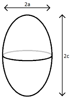
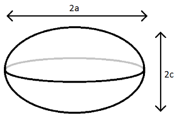
Let us consider a spheroid (ellipsoid with a symmetry of revolution) with axis $\bm{e}_{z}$. Here we do not consider a small perturbation from a sphere anymore, so that we switch to cylindrical coordinates $(\rho,\phi,z)$ that are more convenient for this computation. Let us recall that $\rho$ is the distance to the revolution axis. The vectors of the basis $(\bm{e}_{\rho},\bm{e}_{\phi},\bm{e}_{z})$ have all been defined in the previous section. We denote by $a$ the equatorial radius of the spheroid and by $c$ the distance from the center to the poles (see Fig. 5). In other words, $a$ and $c$ are the two semi-axes of the spheroid. Two cases will be treated separately: the prolate spheroid ($a\leq c$) and the oblate spheroid $(c\leq a)$. More precisely, we detail the computations for the prolate case and only give the results for the oblate case, as the computations are very similar.

Figure 5: A spheroid (ellipsoid of revolution) is defined by two semi-axes: its equatorial radius $a$ and the distance from the center to the poles $c$. Two situations can occur: (left) the prolate spheroid, with $a\leq c$; (right) the oblate spheroid, with $c\leq a$.

For the prolate spheroid, we introduce the eccentricity $e$ as $e=\sqrt{1-(a/c)^{2}}$. Note that $e=0$ corresponds to a sphere of radius $a=c$ and $e=1$ to a stick of length $2c$, oriented along $\bm{e}_{z}$. We have

$$\rho(z)=a\sqrt{1-(z/c)^{2}}\;,$$ (84)

and the surface area of the spheroid is readily computed from

$$S^{\rm prol} =2\pi\int_{-c}^{c}\rho(z)\sqrt{1+\left[\rho^{\prime}(z)\right]^{2}}\,\mathrm{d}{z}$$

$$=2\pi ac\int_{-1}^{1}\sqrt{1-e^{2}x^{2}}\,\mathrm{d}{x}\;,$$ (85)

which yields

$$S^{\rm prol}=2\pi ac\left(\frac{\arcsin(e)}{e}+\sqrt{1-e^{2}}\right)\;.$$ (86)

For an oblate spheroid, the eccentricity is defined as $e=\sqrt{1-(c/a)^{2}}$ and the formula for the surface area becomes

$$S^{\rm obl}=2\pi\left(a^{2}+c^{2}\frac{\operatorname{artanh}(e)}{e}\right)\;.$$ (87)

Now we turn to the computation of $\widetilde{{\mathcal{S}^{(3)}}}$. The outward normal vector is given by

$$(1+\left[\rho^{\prime}(z)\right]^{2})^{-1/2}(\bm{e}_{\rho}+\rho^{\prime}(z)\bm{e}_{z})\;.$$ (88)

First we compute the integral over $\phi$:

$$I(z) =\frac{1}{2\pi}\int_{0}^{2\pi}(\bm{e}_{\rho}+\rho^{\prime}(z)\bm{e}_{z})\otimes(\bm{e}_{\rho}+\rho^{\prime}(z)\bm{e}_{z})\,\mathrm{d}{\phi}$$

$$=\frac{1}{2}\bm{e}_{x}\otimes\bm{e}_{x}+\frac{1}{2}\bm{e}_{y}\otimes\bm{e}_{y}+\left[\rho^{\prime}(z)\right]^{2}\bm{e}_{z}\otimes\bm{e}_{z}\;.$$ (89)

The $\widetilde{{\mathcal{S}^{(3)}}}$ matrix is then given by

$$\widetilde{{\mathcal{S}^{(3)}}}=2\pi\int_{-c}^{c}\rho(z)(1+\rho^{\prime}(z)^{2})^{-1/2}I(z)\,\mathrm{d}{z}\;.$$ (90)

The following computations assume the prolate case. Thanks to the relations

$$\widetilde{{\mathcal{S}^{(3)}}}^{\rm prol}_{xx}=\widetilde{{\mathcal{S}^{(3)}}}^{\rm prol}_{yy}=(S^{\rm prol}-\widetilde{{\mathcal{S}^{(3)}}}^{\rm prol}_{zz})/2\;,$$ (91)

we only have to compute $\widetilde{{\mathcal{S}^{(3)}}}^{\rm prol}_{xx}$ in order to have the full $\widetilde{{\mathcal{S}^{(3)}}}^{\rm prol}$ matrix. We have

$$\widetilde{{\mathcal{S}^{(3)}}}^{\rm prol}_{xx} =\pi ac\int_{-1}^{1}\frac{1-x^{2}}{\sqrt{1-e^{2}x^{2}}}\,\mathrm{d}{x}$$ (92)

$$=2\pi ac\left(\frac{\arcsin{e}}{e}-\frac{1}{2e^{2}}\left(\frac{\arcsin{e}}{e}-\sqrt{1-e^{2}}\right)\right)\;,$$

and then deduce

$$\widetilde{{\mathcal{S}^{(3)}}}^{\rm prol}_{zz}=2\pi ac\left(\frac{\arcsin{e}}{e}-\sqrt{1-e^{2}}\right)\frac{1-e^{2}}{e^{2}}\;.$$ (93)

Using (86), we come to the matrix $\mathcal{S}^{(3)}$ for the prolate spheroid.

In the oblate case, one gets

$$\widetilde{{\mathcal{S}^{(3)}}}^{\rm obl}_{xx}=\pi c^{2}\left(\frac{\operatorname{artanh}{e}}{e}+\frac{1}{e^{2}}\left(\frac{\operatorname{artanh}{e}}{e}-1\right)\right)\;,$$ (94a)

$$\widetilde{{\mathcal{S}^{(3)}}}^{\rm obl}_{zz}=2\pi\left(a^{2}-\frac{c^{2}}{e^{2}}\left(\frac{\operatorname{artanh}{e}}{e}-1\right)\right)\;,$$ (94b)

from which the matrix $\mathcal{S}^{(3)}$ is deduced using (87).

10 Maximal value of $\tau^{(3)}$

In the case of linear gradient encoding in a spherical domain, we obtained that Mitra’s formula is corrected by a factor $\tau^{(3)}$ which is computed from the gradient profile according to Eq. (21). In this section, we investigate the maximum and the minimum values of ${\tau^{(3)}}$. Integrating by parts (following the same procedure as in Eqs. (66)-(68)), one obtains

$${\tau^{(3)}=\frac{3\gamma^{2}}{8b{\color[rgb]{0,0,0}{T}}}\int_{0}^{T}\!\!\int_{0}^{T}q(t_{1})q(t_{2})\left\lvert\frac{t_{1}-t_{2}}{T}\right\rvert^{-1/2}\!\,\mathrm{d}{t_{1}}\,\mathrm{d}{t_{2}}\;.}$$ (95)

Note that despite its singularity at $0$, the function $1/\sqrt{\lvert t\rvert}$ is integrable, hence the above integral is well-defined. Next, we apply a change of variables from $t\in[0,T]$ to $t/T\in[0,1]$ and $q(t)$ to $Q(t/T)$, which gives

$${\tau^{(3)}}=\frac{3}{8{\lVert Q\rVert}^{2}}\int_{0}^{1}\int_{0}^{1}Q(t_{1})Q(t_{2})|t_{1}-t_{2}|^{-1/2}\,\mathrm{d}{t_{1}}\,\mathrm{d}{t_{2}}\;,$$ (96)

with the usual $L_{2}$ norm. One can understand the above expression as a scalar product

$${\tau^{(3)}}=\frac{3}{8}\frac{\langle Q,{\mathcal{K}}Q\rangle}{\langle Q,Q\rangle}\;,$$ (97)

with an integral operator ${\mathcal{K}}$ with the kernel $\lvert t_{1}-t_{2}\rvert^{-1/2}$

$$({\mathcal{K}}Q)(t_{1})=\int_{0}^{1}Q(t_{2})\lvert t_{1}-t_{2}\rvert^{-1/2}\,\mathrm{d}{t_{2}}\;.$$ (98)

One can see that ${\mathcal{K}}$ is a weakly singular convolution operator because the kernel can be expressed as $K(t_{1}-t_{2})$ (with $K(t)=1/\sqrt{\lvert t\rvert}$). Denoting by $\tilde{Q}(\omega)$ the Fourier transform of $Q(t)$ and by $\tilde{K}(\omega)$ the Fourier transform of $K(t)$, one gets

$$\langle Q,{\mathcal{K}}Q\rangle=\frac{1}{2\pi}\int_{-\infty}^{\infty}\lvert\tilde{Q}(\omega)\rvert^{2}\tilde{K}(\omega)\,\mathrm{d}{\omega}\;,$$ (99)

with $\tilde{K}(\omega)=\sqrt{2\pi/\lvert\omega\rvert}$. This shows that ${\tau^{(3)}}$ is always positive (in other words, the operator ${\mathcal{K}}$ is positive-definite). This result is expected from a physical point of view: if ${\tau^{(3)}}$ were negative, then the effective diffusion coefficient would increase with time that is nonphysical. The minimum value $0$ can be asymptotically obtained, for example, with very fast oscillating gradients. It is, indeed, clear from Eq. (99) that if $g(t)$ is a cosine function with angular frequency $\omega_{0}$ such that the number of periods $N_{0}=\omega_{0}T/(2\pi)\gg 1$, then $\lvert\tilde{Q}(\omega)\rvert^{2}$ is concentrated around $\pm\omega_{0}$, and we obtain ${\tau^{(3)}}\approx 3/(8\sqrt{N_{0}}){\sim\omega_{0}^{-1/2}}$, a result that was obtained as well in [16] (see also Fig. 1).

Now we turn to the maximum value of ${\tau^{(3)}}$. The condition that $Q(t)$ is null outside of $[0,1]$ is difficult to take into account in Fourier space and we could not extract further information from Eq. (99). In order to bound the maximum value of ${\tau^{(3)}}$, one can use the Cauchy inequality:

$$\lvert({\mathcal{K}}Q)(t_{1})\rvert=\left\lvert\int_{0}^{1}\sqrt{K(t_{1}-t_{2})}Q(t_{2})\sqrt{K(t_{1}-t_{2})}\,\mathrm{d}{t_{2}}\right\rvert$$

$$\;\leq\left(\int_{0}^{1}K(t_{1}-t_{2})\,\mathrm{d}{t_{2}}\right)^{\frac{1}{2}}\left(\int_{0}^{1}Q^{2}(t_{2})K(t_{1}-t_{2})\,\mathrm{d}{t_{2}}\right)^{\frac{1}{2}}\;.$$

One can easily compute the function

$$\int_{0}^{1}K(t_{1}-t_{2})\,\mathrm{d}{t_{2}}=2\sqrt{t_{1}}+2\sqrt{1-t_{1}}\;,$$ (100)

whose maximum is $2\sqrt{2}$. Thus, one gets

$$\lvert({\mathcal{K}}Q)(t_{1})\rvert\leq\left(2\sqrt{2}\int_{0}^{1}Q^{2}(t_{2})K(t_{1}-t_{2})\,\mathrm{d}{t_{2}}\right)^{\frac{1}{2}}\;.$$ (101)

Using again the Cauchy inequality, one obtains

$$\langle Q,{\mathcal{K}}Q\rangle\leq 2^{3/4}\lVert Q\rVert\left(\int_{0}^{1}\int_{0}^{1}Q^{2}(t_{2})K(t_{1}-t_{2})\,\mathrm{d}{t_{2}}\,\mathrm{d}{t_{1}}\right)^{\frac{1}{2}}\;.$$

The same reasoning about the maximum value of the integral of $K$ yields

$$\langle Q,{\mathcal{K}}Q\rangle\leq 2^{3/2}\lVert Q\rVert^{2}\;,$$ (102)

and finally

$${\tau^{(3)}}\leq\frac{3\sqrt{2}}{4}\approx 1.06\;.$$ (103)

We also know from the examples in Fig. 1 that ${\tau^{(3)}}=1$ can be achieved for $Q\equiv 1$, which implies that the maximum value of ${\tau^{(3)}}$ is in the interval $[1,1.06]$.

The problem can be considered from another point of view. Due to the symmetry of the operator ${\mathcal{K}}$, it is well-known that the function $Q$ maximizing $\langle Q,{\mathcal{K}}Q\rangle/\lVert Q\rVert^{2}$ is the eigenfunction of ${\mathcal{K}}$ with the highest eigenvalue. As a consequence, if one searches for a good estimation of the maximum ${\tau^{(3)}}$ as well as the corresponding “optimal” gradient profile, then one can use the following procedure: (i) to choose an initial profile $Q_{0}$ which is sufficiently general or sufficiently close to a guessed optimal profile; (ii) to apply iteratively the operator ${\mathcal{K}}$ and to renormalize the result; (iii) to stop when the sequence has converged.

For example, the initial profile $Q_{0}(t/T)=1$, which corresponds to two infinitely narrow gradient pulses at time $0$ and $T$, yields ${\tau^{(3)}}=1$, which is close to the optimal value. Thus, it is a good initial condition for the iterative process.

Figure 6: The result of the iterative procedure in order to obtain the optimal profile that maximizes the value of ${\tau^{(3)}}$.

The result of such a procedure is shown in Fig. 6. This yields an optimum value of ${\tau^{(3)}}$ of about $1.006$, thus very close to $1$. It is worth to note, however, that the optimal profile $Q(t/T)$ differs clearly from $Q_{0}(t/T)=1$ (note also that $Q_{0}$ is not an eigenfunction of ${\mathcal{K}}$).

11 Fully isotropic sequence

The conventional condition $\mathcal{T}^{(2)}\propto\mathcal{I}$ removes the microscopic anisotropy in the diffusion tensor, whereas the new isotropy condition $\mathcal{T}^{(3)}\propto\mathcal{I}$ eliminates the mesoscopic anisotropy in the leading order of the short-time expansion. One can thus naturally ask whether it is possible to design a “fully isotropic” sequence that removes anisotropy in all order of $({\color[rgb]{0,0,0}{D_{0}}}T)^{1/2}$? In this appendix we show that it is impossible to find a gradient sequence such that $\mathcal{T}^{(m)}$ is isotropic for all integer values $m=2,3,4,\ldots$. In other words, one cannot find a sequence which produces an isotropic time-dependence of $\,\mathrm{d}(T)$ to every order in $({\color[rgb]{0,0,0}{D_{0}}}T)^{1/2}$. To show this we restrict ourselves to the values of $m$ that are multiple of $4$, $m=4l$, with $l=1,2,\ldots$.

$$\mathcal{T}^{(4l)}_{ij} =-\frac{\gamma^{2}T^{1-2l}}{2b}\int_{0}^{T}\!\!\int_{0}^{T}g_{i}(t_{1})g_{j}(t_{2})(t_{2}-t_{1})^{2l}\,\mathrm{d}{t_{1}}\!\,\mathrm{d}{t_{2}}$$

$$=-\frac{\gamma^{2}T^{1-2l}}{2b}\sum_{k=0}^{2l}(-1)^{k}\binom{2l}{k}\alpha_{i}^{(k)}\alpha_{j}^{(2l-k)}\;,$$ (104)

where

$$\alpha_{i}^{(k)}=\int_{0}^{T}g_{i}(t)t^{k}\,\mathrm{d}{t}\;.$$ (105)

We will now prove that the isotropy of $\mathcal{T}^{(4l)}$ for any integer $l$ implies that $\alpha_{i}^{(k)}=0$ for all $i=x,y,z$ and all integer $k$. Note that the property for $k=0$ corresponds to the refocusing condition (4) that we assumed throughout the paper. We prove our statement by recurrence on $l$ and $k$. First, let us consider $l=1$ and prove the $k=1$ case. One has

$$\mathcal{T}^{(4)}_{ij}=-\frac{\gamma^{2}T^{-1}}{2b}\left(-2\alpha_{i}^{(1)}\alpha_{j}^{(1)}\right)\;.$$ (106)

If $i\neq j$, then $\mathcal{T}^{(4)}_{ii}=\mathcal{T}^{(4)}_{jj}$ and $\mathcal{T}^{(4)}_{ij}=0$ so that $\alpha_{i}^{(1)}=\alpha_{j}^{(1)}=0$.

Now we assume that $\alpha_{i}^{(k)}=0$ for all $i=x,y,z$ and for all $k<k^{\prime}$ up to a given rank $k^{\prime}$. Then almost all the terms in the expression of $\mathcal{T}^{(4k^{\prime})}_{ij}$ vanish and we are left with

$$\mathcal{T}^{(4k^{\prime})}_{ij}=-\frac{\gamma^{2}T^{1-2k^{\prime}}}{2b}\left((-1)^{k^{\prime}}\binom{2k^{\prime}}{k^{\prime}}\alpha_{i}^{(k^{\prime})}\alpha_{j}^{(k^{\prime})}\right)\;,$$ (107)

and with the same reasoning as in the previous case, we deduce that $\alpha_{i}^{(k^{\prime})}=0$ for any $i$. By recurrence, we have proven that $\alpha_{i}^{(k)}=0$ for all $i$ and $k$.

What remains to prove is that the only continuous function $f(t)$ that satisfies $\int_{0}^{T}f(t)t^{k}\d{t}=0$ for all integer values of $k$ is the null function $f=0$. Let us assume that $f$ is nonzero, i.e., there exists an interval $(a,b)$ with $a<b$ such that $f(t)\neq 0$ for any $t\in(a,b)$ (e.g., $f(t)>0$ on this interval). Since polynomials form a dense subset of continuous functions on $[0,T]$, one can build a sequence of polynomials that converges to a continuous function that would be zero outside $(a,b)$ and positive inside $(a,b)$. Thus there would exist a polynomial $P(t)$ such that $\int_{0}^{T}f(t)P(t)\,\mathrm{d}{t}>0$, which is incompatible with the statement: for all $k=0,1,2,\ldots$ $\int_{0}^{T}f(t)t^{k}\,\mathrm{d}{t}=0$. Note that this argument can be easily extended to functions with a finite number of jumps.

References

- [1] P. P. Mitra, P. N. Sen, L. M. Schwartz, and P. Le Doussal, “Diffusion propagator as a probe of the structure of porous media,” Phys. Rev. Lett., vol. 68, pp. 3555–3558, 1992.
- [2] P. P. Mitra and P. N. Sen, “Effects of microgeometry and surface relaxation on NMR pulsed-field-gradient experiments: Simple pore geometries,” Phys. Rev. B, vol. 45, pp. 143–156, 1992.
- [3] P. P. Mitra, P. N. Sen, and L. M. Schwartz, “Short-time behavior of the diffusion coefficient as a geometrical probe of porous media,” Phys. Rev. B, vol. 47, pp. 8565–8574, 1993.
- [4] L. L. Latour, P. P. Mitra, R. L. Kleinberg, and C. H. Sotak, “Time-dependent diffusion coefficient of fluids in porous media as a probe of surface-to-volume ratio,” J. Magn. Res. A, vol. 101, no. 3, pp. 342 – 346, 1993.
- [5] K. G. Helmer, B. J. Dardzinski, and C. H. Sotak, “The application of porous-media theory to the investigation of time-dependent diffusion in in vivo systems,” NMR Biomed., vol. 8, no. 7, pp. 297–306, 1995.
- [6] K. G. Helmer, M. D. Hürlimann, T. M. de Swiet, P. N. Sen, and C. H. Sotak, “Determination of ratio of surface area to pore volume from restricted diffusion in a constant field gradient,” J. Magn. Res. A, vol. 115, no. 2, pp. 257–259, 1995.
- [7] P. N. Sen, “Time-dependent diffusion coefficient as a probe of geometry,” Conc. Magn. Res. A, vol. 23A, no. 1, pp. 1–21, 2004.
- [8] D. S. Grebenkov, “NMR survey of reflected Brownian motion,” Rev. Mod. Phys., vol. 79, pp. 1077–1137, 2007.
- [9] E. O. Stejskal and J. E. Tanner, “Spin diffusion measurements: Spin echoes in the presence of a time-dependent field gradient,” J. Chem. Phys., vol. 42, no. 1, pp. 288–292, 1965.
- [10] E. J. Fordham, S. J. Gibbs, and L. D. Hall, “Partially restricted diffusion in a permeable sandstone: Observations by stimulated echo PFG NMR,” Magn. Reson. Imaging, vol. 12, no. 2, pp. 279–284, 1994. Proceedings of the Second International Meeting on Recent Advances in MR Applications to Porous Media.
- [11] M. D. Hürlimann, K. G. Helmer, L. L. Latour, and C. H. Sotak, “Restricted diffusion in sedimentary rocks. Determination of surface-area-to-volume ratio and surface relaxivity,” J. Magn. Res. A, vol. 111, no. 2, pp. 169–178, 1994.
- [12] L. L. Latour, K. Svoboda, P. P. Mitra, and C. H. Sotak, “Time-dependent diffusion of water in a biological model system.,” PNAS, vol. 91, no. 4, pp. 1229–1233, 1994.
- [13] R. W. Mair, G. P. Wong, D. Hoffmann, M. D. Hürlimann, S. Patz, L. M. Schwartz, and R. L. Walsworth, “Probing porous media with gas diffusion NMR,” Phys. Rev. Lett., vol. 83, pp. 3324–3327, 1999.
- [14] M. Carl, G. W. Miller, J. P. Mugler, S. Rohrbaugh, W. A. Tobias, and G. D. Cates, “Measurement of hyperpolarized gas diffusion at very short time scales,” J. Magn. Reson., vol. 189, no. 2, pp. 228 – 240, 2007.
- [15] T. M. de Swiet and P. N. Sen, “Decay of nuclear magnetization by bounded diffusion in a constant field gradient,” J. Chem. Phys., vol. 100, no. 8, pp. 5597–5604, 1994.
- [16] D. S. Novikov and V. G. Kiselev, “Surface-to-volume ratio with oscillating gradients,” J. Magn. Reson., vol. 210, no. 1, pp. 141 – 145, 2011.
- [17] G. Lemberskiy, S. H. Baete, M. A. Cloos, D. S. Novikov, and E. Fieremans, “Validation of surface-to-volume ratio measurements derived from oscillating gradient spin echo on a clinical scanner using anisotropic fiber phantoms,” NMR Biomed., vol. 30, no. 5, p. e3708, 2017.
- [18] A. F. Frølich, S. N. Jespersen, L. Østergaard, and V. G. Kiselev, “The effect of impermeable boundaries of arbitrary geometry on the apparent diffusion coefficient,” J. Magn. Reson., vol. 194, pp. 128–135, 2008.
- [19] P. J. Basser, J. Mattiello, and D. Le Bihan, “Estimation of the effective self-diffusion tensor from the NMR spin echo,” J. Magn. Res. B, vol. 103, no. 3, pp. 247–254, 1994.
- [20] J. Mattiello, P. J. Basser, and D. Le Bihan, “Analytical expressions for the b Matrix in NMR diffusion imaging and spectroscopy,” J. Magn. Res. A, vol. 108, no. 2, pp. 131–141, 1994.
- [21] P. J. Basser, J. Mattiello, and D. Le Bihan, “MR diffusion tensor spectroscopy and imaging,” Biophys. J., vol. 66, no. 1, pp. 259 – 267, 1994.
- [22] P. J. Basser and D. K. Jones, “Diffusion-tensor MRI: theory, experimental design and data analysis: a technical review,” NMR Biomed., vol. 15, no. 7-8, pp. 456–467, 2002.
- [23] S. Lasič, F. Szczepankiewicz, S. Eriksson, M. Nilsson, and D. Topgaard, “Microanisotropy imaging: quantification of microscopic diffusion anisotropy and orientational order parameter by diffusion MRI with magic-angle spinning of the q-vector,” Front. Phys., vol. 2, p. 11, 2014.
- [24] F. Szczepankiewicz, S. Lasič, D. van Westen, P. C. Sundgren, E. Englund, C.-F. Westin, F. Ståhlberg, J. Lätt, D. Topgaard, and M. Nilsson, “Quantification of microscopic diffusion anisotropy disentangles effects of orientation dispersion from microstructure: Applications in healthy volunteers and in brain tumors,” Neuroimage, vol. 104, pp. 241 – 252, 2015.
- [25] C.-F. Westin, H. Knutsson, O. Pasternak, F. Szczepankiewicz, E. Özarslan, D. van Westen, C. Mattisson, M. Bogren, L. J. O’Donnell, M. Kubicki, D. Topgaard, and M. Nilsson, “Q-space trajectory imaging for multidimensional diffusion MRI of the human brain,” Neuroimage, vol. 135, pp. 345 – 362, 2016.
- [26] S. N. Jespersen, J. L. Olesen, A. Ianuş, and N. Shemesh, “Effects of nongaussian diffusion on “isotropic diffusion” measurements: An ex-vivo microimaging and simulation study,” J. Magn. Reson., vol. 300, pp. 84–94, 2019.
- [27] Y. Cheng, and D. G. Cory, “Multiple scattering by NMR” J. Am. Chem. Soc., vol. 121, no. 34, pp. 7935–7936, 1999.
- [28] P. P. Mitra, “Multiple wave-vector extensions of the NMR pulsed-field-gradient spin-echo diffusion measurement,” Phys. Rev. B, vol. 51, pp. 15074–15078, 1995.
- [29] N. Shemesh, S. N. Jespersen, D. C. Alexander, Y. Cohen, I. Drobnjak, T. B. Dyrby, J. Finsterbusch, M. A. Koch, T. Kuder, F. Laun, M. Lawrenz, H. Lundell, P. P. Mitra, M. Nilsson, E. Özarslan, D. Topgaard, C.-F. Westin, “Conventions and nomenclature for double diffusion encoding NMR and MRI” Magn. Res. Med., vol. 75, pp. 82–87, 2015.
- [30] S. Mori and P. C. M. Van Zijl, “Diffusion weighting by the trace of the diffusion tensor within a single scan,” Magn. Reson. Med., vol. 33, no. 1, pp. 41–52, 1995.
- [31] E. C. Wong, R. W. Cox, and A. W. Song, “Optimized isotropic diffusion weighting,” Magn. Res. Med., vol. 34, no. 2, pp. 139–143, 1995.
- [32] R. A. de Graaf, K. P. J. Braun, and K. Nicolay, “Single-shot diffusion trace NMR spectroscopy,” Magn. Res. Med., vol. 45, no. 5, pp. 741–748, 2001.
- [33] J. Valette, C. Giraudeau, C. Marchadour, B. Djemai, F. Geffroy, M. A. Ghaly, D. Le Bihan, P. Hantraye, V. Lebon, and F. Lethimonnier, “A new sequence for single-shot diffusion-weighted NMR spectroscopy by the trace of the diffusion tensor,” Magn. Res. Med., vol. 68, no. 6, pp. 1705–1712, 2012.
- [34] S. Eriksson, S. Lasič, and D. Topgaard, “Isotropic diffusion weighting in PGSE NMR by magic-angle spinning of the q-vector,” J. Magn. Reson., vol. 226, pp. 13 – 18, 2013.
- [35] D. Topgaard, “Isotropic diffusion weighting in PGSE NMR: Numerical optimization of the q-MAS PGSE sequence,” Microporous Mesoporous Mater., vol. 178, pp. 60 – 63, 2013. Proceedings of the 11th Internatioanl Bologna Conference on Magnetic Resonance in Porous Media (MRPM11).
- [36] D. Topgaard “Multidimensional diffusion MRI,” J. Magn. Reson., vol. 275, pp. 98–113, 2017.
- [37] J. P. de Almeida Martins and D. Topgaard, “Two-dimensional correlation of isotropic and directional diffusion using NMR,” Phys. Rev. Lett., vol. 116, p. 087601, 2016.
- [38] R. F. Karlicek and I. J. Lowe, “A modified pulsed gradient technique for measuring diffusion in the presence of large background gradients,” J. Magn. Res. (1969), vol. 37, no. 1, pp. 75–91, 1980.
- [39] S. Axelrod and P. N. Sen, “Nuclear magnetic resonance spin echoes for restricted diffusion in an inhomogeneous field: Methods and asymptotic regimes,” J. Chem. Phys., vol. 114, no. 15, pp. 6878–6895, 2001.
- [40] D. S. Grebenkov, “Laplacian eigenfunctions in NMR. II. Theoretical advances,” Conc. Magn. Res. A, vol. 34A, no. 5, pp. 264–296, 2009.
- [41] G. Lemberskiy, A. B. Rosenkrantz, J. Veraart, S. S. Taneja, D. S. Novikov, E. Fieremans, “Time-dependent diffusion in prostate cancer,” Invest. Radiol., vol. 52, pp. 405-411, 2017.
- [42] D. A. Yablonskiy, A. L. Sukstanskii, J. C. Leawoods, D. S. Gierada, G. L. Bretthorst, S. S. Lefrak, J. D. Cooper, and M. S. Conradi, “Quantitative in vivo Assessment of Lung Microstructure at the Alveolar Level with Hyperpolarized 3He Diffusion MRI,” PNAS, vol. 99, p. 3111, 2002.
- [43] G. G. Cleveland, D. C. Chang, C. F. Hazelwood, and H. E. Rorschach, “Nuclear magnetic resonance measurement of skeletal muscle: Anisotropy of the diffusion coefficient of the intracellular water,” Biophys. J., vol. 16, pp. 1043–1053, 1976.
- [44] P. van Gelderen, D. Despres, P. C. M. Vanzijl, and C. T. W. Moonen, “Evaluation of restricted diffusion in cylinders. Phosphocreatine in rabbit leg muscle,” J. Magn. Res. B, vol. 103, pp. 255–260, 1994.
- [45] J. Oudeman, A. J. Neverdeen, G. J. Strijkers, M. Maas, P. R. Luijten, and M. Froeling, “Techniques and applications of skeletal muscle diffusion tensor imaging: A review,” J. Magn. Reson. Imaging, vol. 43, pp. 773–788, 2016.
- [46] M. Tariq, T. Schneider, D. C. Alexander, C. A. G. Wheeler-Kingshott, and H. Zhang, “Bingham–NODDI: Mapping anisotropic orientation dispersion of neurites using diffusion MRI,” NeuroImage, vol. 133, pp. 207–223, 2016.
- [47] H. Zhang, P. L. Hubbard, G. J. M. Parker, and D. C. Alexander, “Axon diameter mapping in the presence of orientation dispersion with diffusion MRI,” NeuroImage, vol. 56, pp.8 1301–1315, 2011.
- [48] D. S. Grebenkov, “Diffusion MRI/NMR at high gradients: Challenges and perspectives,” Microporous Mesoporous Mater., vol. 269, pp. 79–82, 2018.
- [49] S. N. Jespersen, H. Lundell, C. K. Sønderby, and T. B. Dyrby, “Orientationally invariant metrics of apparent compartment eccentricity from double pulsed field gradient diffusion experiments,” NMR Biomed., vol. 26, pp. 1647–1662, 2013.
- [50] S. Vellmer, R. Stirnberg, D. Edelhoff, D. Suter, T. Stöcker, and I. I. Maximov, “Comparative analysis of isotropic diffusion weighted imaging sequences,” J. Magn. Reson., vol. 275, pp. 137 – 147, 2017.
- [51] P. M. Pattany, J. J. Phillips, L. C. Chiu, J. D. Lipcamon, J. L. Duerk, J. M. McNally, and S. N. Mohapatra, “Motion artifact suppresion technique (MAST) for MR imaging,” J. Comput. Assisted Tomogr., vol. 11, pp. 369–377, 1987.
- [52] F. B. Laun, T. A. Kuder, F. Zong, S. Hertel, and P. Galvosas, “Symmetry of the gradient profile as second experimental dimension in the short-time expansion of the apparent diffusion coefficient as measured with NMR diffusometry,” J. Magn. Reson., vol. 259, pp. 10 – 19, 2015.
- [53] F. B. Laun, K. Demberg, A. M. Nagel, M. Uder, and T. Kuder, “On the Vanishing of the t-term in the Short-Time Expansion of the Diffusion Coefficient for Oscillating Gradients in Diffusion NMR,” Front. Phys., vol. 5, pp. 56, 2017.
- [54] E. B. Davies, Heat Kernels and Spectral Theory. Cambridge Tracts in Mathematics, Cambridge University Press, 1989.
- [55] P. Gilkey, Asymptotic Formulae in Spectral Geometry. Chapman and Hall/CRC, 2003.
- [56] S. Desjardins and P. Gilkey, “Heat content asymptotics for operators of Laplace type with Neumann boundary conditions,” Math. Z., vol. 215, pp. 251–268, 1994.
- [57] J. Xu, M. D. Does, and J. C. Gore, “Dependence of temporal diffusion spectra on microstructural properties of biological tissues,” Magn. Reson. Imag., vol. 29, pp. 380-–390, 2011.
- [58] O. Reynaud, “Time-Dependent Diffusion MRI in Cancer: Tissue Modeling and Applications,” Front. Phys., vol. 5, p. 58, 2017.
- [59] P. J. Basser, “Inferring microstructural features and the physiological state of tissues from diffusion-weighted images,” NMR BioMed., vol. 8, no. 7, pp. 333–344, 1995.