Transition-region explosive events produced by plasmoid instability

Abstract

Magnetic reconnection is thought to be a key process in most of solar eruptions. Thanks to high-resolution observations and simulations, the studied scale of reconnection process has become smaller and smaller. Spectroscopic observations show that the reconnection site can be very small, which always exhibits a bright core and two extended wings with fast speeds, i.e., transition-region explosive events. In this paper, using the PLUTO code, we perform a 2-D magnetohydrodynamic simulation to investigate the small-scale reconnection in double current sheets. Based on our simulation results, such as the line-of-sight velocity, number density and plasma temperature, we can synthesize the line profile of Si iv 1402.77 Å which is a well known emission line to study the transition-region explosive events on the Sun. The synthetic line profile of Si iv 1402.77 Å is complex with a bright core and two broad wings which can extend to be nearly 200 km s^-1. Our simulation results suggest that the transition-region explosive events on the Sun are produced by plasmoid instability during the small-scale magnetic reconnection.

1 Introduction

The break and re-join of magnetic fields are generally thought to be the process of magnetic reconnection. It is always believed as a basic process of energy release on the Sun, and usually accompanied by the particle acceleration. Almost all the solar eruptions which are related with the magnetic energy release are thought to be associated with magnetic reconnection, i.e., coronal mass ejections (Lin et al., 2005; Guo et al., 2013), emerging flux regions (Zhao & Li, 2012; Yang & Zhang, 2014), bipolar magnetic regions (Jiang et al., 2014; Li, 2017), solar flares (Petschek, 1964; Liu et al., 2010; Yan et al., 2018), solar filaments (Shen et al., 2015; Li et al., 2016a; Li & Ding, 2017), bright points (Priest et al., 1994; Li & Ning, 2012; Zhao et al., 2017), and transition-region explosive events (Innes et al., 1997; Ning et al., 2004; Huang et al., 2017). That is to say, the Sun can provide various observational features of magnetic reconnection in a wide range of scales, i.e., from $\sim$1000 Mm to $\sim$1 Mm. The diagnostics of magnetic reconnection often depend on the imaging observations (Masuda et al., 1994; Tian et al., 2014; Xue et al., 2016), the spectroscopic observations (Curdt & Tian, 2011; Cheng et al., 2015; Li et al., 2018; Tian et al., 2018), and also the magnetohydrodynamic (MHD) simulations (Jin et al., 1996; Khomenko & Collados, 2012; Yang et al., 2015a). Over the past few decades, many observational features have been identified as the evidences of magnetic reconnection on the Sun, such as the X-type structures (Aschwanden, 2002; Su et al., 2013; Yang et al., 2015b), the magnetic null point (Sun et al., 2012; Zhang et al., 2012), the current sheets (Lin et al., 2005; Liu et al., 2010; Xue et al., 2018), the reconnection inflows or outflows (Liu et al., 2013; Ning & Guo, 2014; Sun et al., 2015; Li et al., 2016b), the high-energetic particles (Li et al., 2007, 2009; Klassen et al., 2011), and also the bi-directional jets (Dere et al., 1991; Winebarger et al., 2002; Innes & Teriaca, 2013; Hong et al., 2016).

Transition-region explosive events are detected frequently in the quiet or active Sun. They usually display as the broad non-Gaussian profiles with a high velocity of about 100 $km~{}s^{-1}$ in the emission lines, i.e., Si iv 1393 Å (Innes et al., 1997; Ning et al., 2004) and 1402.77 Å (Huang et al., 2014; Innes et al., 2015), C iv 1548 Å and O iv 1032 Å (Pérez et al., 1999; Innes & Teriaca, 2013). Usually, these emission lines are formed between 6$\times$10${}^{4}~{}K$ (e.g., C iii) and 7$\times$10${}^{5}~{}K$ (e.g., Ne viii) (Wilhelm et al., 2007) in the transition regions. The transition-region explosive events were firstly detected by the spectra from High-Resolution Telescope and Spectrograph (HRTS) observations (Brueckner & Bartoe, 1983), and then described in more detailed by Dere et al. (1989) and Dere (1994). Their typical size is found to be about 1500 km, and the lifetime is around 60 s. Spectroscopic observations (e.g., Dere et al., 1989; Innes et al., 1997; Ning et al., 2004) further show that they are always exhibiting a line asymmetry, i.e., the extended blue or red wings, whose typical speed can be $\sim$100 $km~{}s^{-1}$. The single event observed by a line profile often exhibits the blue and red shifts simultaneously, which is regarded as the small-scale jet with bi-directions in the transition region, and it is thought to be associated with the small-scale magnetic reconnection on the Sun (Innes et al., 1997).

MHD numerical simulations have been applied to the magnetic reconnection in the corona (Shen et al., 2011; Ni et al., 2012), the transition region (e.g., Innes & Tóth, 1999; Sarro et al., 1999; Roussev et al., 2001), and the chromosphere or even the photosphere (Ni et al., 2015, 2016) on the Sun. Previous simulations of the transition-region explosive events were often based on the Petschek mechanism (Petschek, 1964). The upward and downward motions of magnetic islands were thought to be associated with the blue and red shifts in the explosive events (Jin et al., 1996). Further simulation (Roussev et al., 2001) indicated that the reconnection with an X-point in the transition region produced a large blue shift ($\sim$100 $km~{}s^{-1}$), but a small red shift. Meanwhile, Innes & Tóth (1999) performed a compressible MHD simulations of the small-scale explosive events based on the Petschek model, and they found that the simulations could well reproduce the blue or red shifts with high velocities, but failed to explain the bright core near the line center with low velocities observed by the spectra (e.g., Dere et al., 1991; Innes, 2001). Based on the large-scale MHD simulations (e.g., Bhattacharjee et al., 2009; Heggland et al., 2009; Huang & Bhattacharjee, 2010; Huang et al., 2017), the magnetic reconnection proceeds via the plasmoid instability has been proposed. Now, this model has also been applied to explain the small-scale explosive events which exhibit the brightening both at spectral line core and two extended wings, i.e., the line profile of Si iv 1402.77 Å (e.g., Innes et al., 2015).

In this paper, we perform a 2-D MHD simulation of magnetic reconnection at a small scale which is produced in double current sheets with the PLUTO code (Mignone et al., 2007, 2012). We also synthesize the line profiles which formed in the transition region, i.e., Si iv 1402.77 Å (Tian, 2017). Our result suggests that the transition-region explosive events on the Sun are the small-scale reconnection sites, which is consistent with the IRIS (De Pontieu et al., 2014) observations (see., Innes et al., 2015).

2 Numerical method

2.1 MHD simulation

In this paper, the PLUTO code (Mignone et al., 2007) with adaptive mesh refinement (AMR) (Mignone et al., 2012) is applied to perform the MHD simulation. Briefly, a Newtonian fluid with density ($\rho$), velocity ($\mathbf{v}$) and magnetic field ($\mathbf{B}$) is considered, then the forms of single-fluid MHD Equations are

$$\frac{\partial\rho}{\partial t}+\nabla\cdot(\rho\mathbf{v}) = 0,$$

$$\frac{\partial(\rho\mathbf{v})}{\partial t}+\nabla\cdot(\rho\mathbf{v}\mathbf{v}-\mathbf{B}\mathbf{B})+\nabla p_{t} = 0,$$ (1)

$$\frac{\partial E}{\partial t}+\nabla\cdot[(E+p_{t})\mathbf{v}-(\mathbf{v}\cdot\mathbf{B})\mathbf{B}] = -\eta\cdot\mathbf{J}\times\mathbf{B}-\Lambda,$$

$$\frac{\partial\mathbf{B}}{\partial t}-\nabla\times(\mathbf{v}\times\mathbf{B}) = -\nabla\times(\eta\mathbf{J}).$$

where $p_{t}=p+\mathbf{B}^{2}/2$ is the total pressure which consists of thermal and magnetic pressures. $E=p/(\gamma-1)+\frac{1}{2}\rho\mathbf{v}^{2}+\frac{1}{2}\mathbf{B}^{2}$ is the total energy density at the ideal state, and $\gamma$ is the specific heat ratio. $\mathbf{J}=\nabla\times\mathbf{B}$ is the electric current density, and $\eta$ is the resistivity. Our simulation considers the Ohmic heating and optically thin radiative cooling (see., equation 2), but the dissipative effects caused by the viscous and gravity are ignored. Notice that only the hydrogen gas is considered in our 2-D MHD model.

$$\Lambda=n^{2}\tilde{\Lambda}(T),\quad\mbox{with}\quad n=\frac{\rho}{\mu m_{u}}.$$ (2)

Here $n$ is the number density, $\mu$ is the mean molecular weight, and $m_{u}$ is the atomic mass unit. In our model, the cooling rates ($\tilde{\Lambda}$) are discrete as a table sampled. Figure 1 gives the cooling rates (see., Mignone et al., 2007) used in this paper.

Figure 1: Tabulated cooling rates in log$-$log space, the data is derived from Mignone et al. (2007).

In our simulation, we consider a Cartesian 2-D uniform grid x, y $\in$ [0, 2], with 64 $\times$ 64 zones at the coarse level, and with periodic boundary conditions along all the two directions. To trigger the magnetic reconnection, the initial magnetic field is defined only in the vertical (Y) direction, as shown in equation 3 with $B=1.0$ (see., Mignone et al., 2012).

$$B_{y}=\left\{\begin{array}[]{l}-B~{}~{}~{}~{}~{}~{}\quad\mbox{if}\quad|x-1|\leq 0.5,\\ ~{}~{}B~{}~{}~{}~{}~{}~{}\qquad\mbox{otherwise}.\end{array}\right.$$ (3)

In X direction, a small initial perturbation to the velocity is set to start the reconnection, i.e., $v_{x}=0.1\times\ v_{0}sin(\pi\cdot y$). The initial thermal pressure is given by the magnetic filed and plasma beta ($\beta$), such as $p=\beta\cdot B^{2}/2$. The MHD fluid has an uniform density at the initial beginning, which is $\rho=1.0$. The temperate can be obtained from the density and thermal pressure in the code, i.e., $T=p/\rho$. In order to obtain the high-resolution grid and save the computing time, the AMR is allowed for the MHD simulation. The four-level refinement is activated for carrying out the integration with the TVDLF solver. Finally, we perform the reconstruction on characteristic variables rather than primitive values and set the monotonized central difference limiter (MC_LIM). In the whole simulation, we assume an ideal gas state with the specific heat ratio ($\gamma$) of 5/3, and the mean molecular weight ($\mu$) of 1/2.

Generally speaking, PLUTO is working with the non-dimensional (or code) unit, which is described above. However, we have considered the radiative cooling process, and the dimensional constants are essential to scale data values to physical units. Thus, we have to introduce the specific length and energy scale so that they can compare with the dynamical advection scales. Therefore, we can specify three fundamental units, they are the length ($L_{0}$), the velocity ($v_{0}$), and the number density ($n_{0}$) which is corresponding to the mass density of $\rho_{0}=n_{0}m_{u}$. The other units can be derived from these three fundamental units, such as time $t_{0}=L_{0}/v_{0}$, pressure $p_{0}=\rho_{0}v_{0}^{2}$, magnetic field $B_{0}=v_{0}\sqrt{4\pi\rho_{0}}$, and temperature $T_{0}=\mu m_{u}v_{0}^{2}/k_{B}$, where $k_{B}$ is the Boltzmann constant. Noting that all these dimensional units are c.g.s, i.e., $cm$, $s$, and $gr$. During the entire process of MHD simulation, an uniform resistivity ($\eta$) is employed.

Table 1 lists the characteristic and initial values of these fundamental units in our 2-D simulation. The characteristic length is set to be 10${}^{8}~{}cm$, and thus the simulation box has a size of 2$\times$2 Mm. The characteristic number density and velocity are set to be 10${}^{10}~{}cm^{-3}$ and 2$\times$10${}^{7}~{}cm~{}s^{-1}$ at first, respectively, which leads to a characteristic plasma beta of $\beta\approx 1.67$, as shown in the second lines (CPs) of table 1. Therefore, the MHD flows have an initial uniform density of 10${}^{10}~{}cm^{-3}$, the initial magnetic field of about 10 $G$, and a small initial perturbation velocity of 2$\times$10${}^{6}~{}cm~{}s^{-1}$, this gives an initial plasma beta of $\beta\approx 0.02$, as indicated in the third lines (IPs) of table 1. Finally, an uniform resistivity ($\eta$ = 10^-5) is performed.

Table 1: The characteristic parameters (CPs) and the initial parameters (IPs) in our 2-D MHD simulations.

	$L_{0}$ (cm)	$n_{0}$ (cm-3)	$v_{0}$ (cm s-1)	$T_{0}$ (K)	$B_{0}$ (G)	$\beta$	$\eta$
CPs	108	1010	2$\times$107	2.4$\times$106	$\sim$10	1.67	10-5
IPs	108	1010	2$\times$106	2.4$\times$104	$\sim$10	0.02	10-5

2.2 Line synthesis

The values of six variables, such as the number density($n$), the total energy (E), the velocities ($v_{x}$, $v_{y}$) and the magnetic fields (B_x, B_y) are derived at each time step by solving the 2-D MHD equations, then the plasma temperature ($T$) can be derived by using the values of these variables. Using these variables, and assuming that the emission line is made up with a group of Gaussian profiles, we can synthesize the line profile with equation 4 (see also., Hansteen et al., 2010; Yuan et al., 2016), i.e., Si iv 1402.77 Å, which is a well known spectral line to study the transition-region explosive events from IRIS observations (e.g., Innes et al., 2015).

$$I(v)=\frac{\Sigma}{4\pi R_{AU}^{2}}\int{\phi(v_{s})~{}n_{e}~{}n~{}g(T)}ds.$$ (4)

Here the integral intensity of spectral line is carried out along the chosen light-of-sight (LOS). $n_{e}$ is the electron number density, and assuming that $n_{e}=n$, $\Sigma$ is the area of the MHD simulation region, $R_{AU}$ is the distance between the Sun and the Earth, $\frac{\Sigma}{4\pi R_{AU}^{2}}$ represent the ratio between the spectral line intensity which radiate from the Sun and that we have received on the Earth (e.g., Winebarger et al., 1999). $g(T)$ is the contribution function of the specified emission line, i.e., Si iv 1402.77 Å, which can be obtained from the CHIANTI database version 8.0 (Del Zanna et al., 2015). $\phi(v_{s})$ is a Gaussian function with a variable of $v_{s}$ (the unit of velocity is $km~{}s^{-1}$ here), see., equation 5.

$$\phi(v_{s})=\frac{1}{\sqrt{\pi}\Delta v_{D}}e^{-\frac{(v-v_{s})^{2}}{2\Delta v_{D}^{2}}},\quad\mbox{with}\quad\Delta v_{D}=\sqrt{\frac{2k_{B}T}{m}}.$$ (5)

Where $\Delta v_{D}$ represents the thermal broadening from the simulation temperature $T$, and $m$ is the mass of the radiating ion, while $v_{s}$ is the fluid speed projected along the LOS direction, i.e., the velocity in y-direction ($v_{y}$) from the numerical results, as shown in Figure 2.

3 Results

3.1 MHD simulation results

Figure 2 shows the variables which derived from our 2-D MHD simulation at t = 22 s. The upper panels gives the simulation variables without radiative cooling process, such as the velocities along Y direction ($v_{y}$), the plasma temperature ($T$), and the number density ($n_{e}$). All these simulation variables show that every magnetic island includes an O-point in its center and a pair of X-point at its sides. These magnetic islands in the double current sheets interact with each other. The Joule heating and shocks inside these islands are the possible mechanisms to heat the plasmas (Ni et al., 2015, 2016), and could further produce the bright core and extended enhanced wings (Innes et al., 2015). The velocities at two sides of magnetic islands can be reached a fast speed of around 200 $km~{}s^{-1}$, whatever the blue or red shifts, while the velocities in the centers of magnetic islands is slow, as shown in panel (a). However, the plasma temperature is very high in the double current sheets, especially in the magnetic islands. The plasma temperature in the center and two sides of magnetic islands can be as high as 10${}^{6}~{}K$ (panel b), which is much higher than the formation temperature of Si iv 1402.77 Å, i.e., 8$\times$10${}^{4}~{}K$. Therefore, we expect the radiative cooling process to decrease the temperature inside the reconnection region, as seen $\Lambda$ in equation 1.

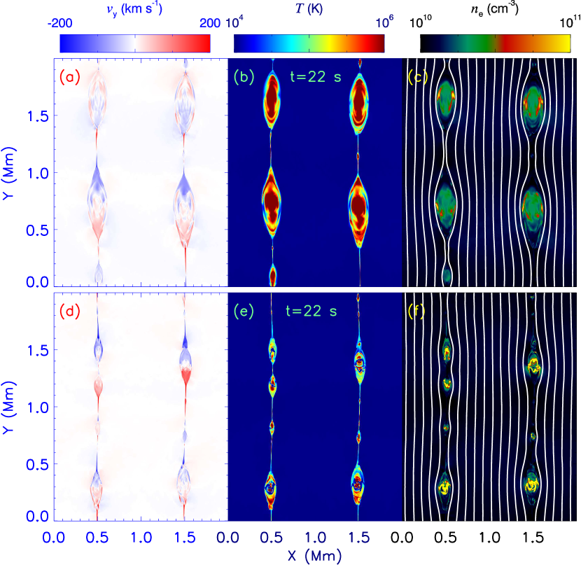
Figure 2: The MHD simulation results without (upper) and with (bottom) cooling process at t = 22 s: velocity (a, d), plasma temperature (b, e), and number density (c, f). The white profiles represent the magnetic field lines.

The cooling function is defined by the number density ($n$) and cooling rates (see., equation 2), while the cooling rates ($\tilde{\Lambda}$) are from the table which given by Mignone et al. (2007). Figure 1 shows the cooling rates depend on the temperature, which clearly shows that the cooling rates are strongly sensitive to the temperature between about 10${}^{4}~{}K$ and 10${}^{6}~{}K$. This is just what we are interested, as the formation temperature of Si iv 1402.77 Å is exactly between them. In fact, the cooling rates are also sensitive at much higher temperature, i.e., $>10^{8}~{}K$, but it is out of scope of this study.

The bottom panels in Figure 2 show the MHD simulation results with the radiative cooling process at t = 22 s. Similar as the upper panels in Figure 2, multiple magnetic islands with O-points in their centers and X-points at their two sides appear, they are interact with each other. The velocities at two sides of magnetic islands can be around 200 $km~{}s^{-1}$, while the velocities in the centers of magnetic islands is slow, as shown in panel (d). Moreover, the plasma temperature in the reconnection region are decreasing, but the number density is increasing at the same time. The plasma temperature in the double current sheets is cooling down to form the Si iv 1402.77 Å line, i.e., in the centers and two sides of the magnetic islands.

3.2 Synthesis line profiles

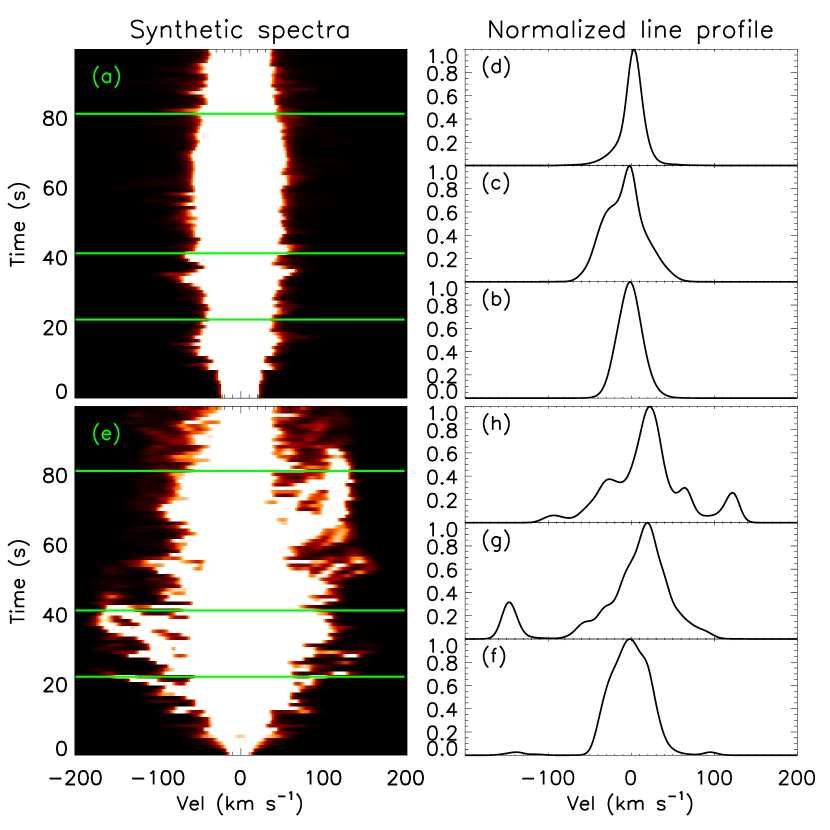
Figure 3: Line profiles obtained from the 2-D MHD simulations. Left: time evolution of the line profiles of Si iv 1402.77 Å without (a) and with (e) the cooling process. Right: Line profiles indicated by the green horizontal lines on the left panel.

Using equation 4 and the simulation variables, we can synthesize the line profiles of Si iv 1402.77 Å, as shown in Figure 3. Here, the velocity distribution (Vel) is the velocity (v) on the left side of equation (4), and the final value of the intensity for each given v (Vel) as shown in Figure 3 is then calculated by adding all the integral intensity I(v) at each X point. Panel (e) shows the evolution of the spectral line with time in the case with radiative cooling. At the beginning of t $\approx$ 0$-$5 s, only the line core is bright, and it is also very narrow. Then the line core becomes broader and broader with time, such as at t $\approx$ 5$-$15 s. Next, two extended line wings appear to brighten and move to blue and red wings simultaneously, i.e., t $\approx$ 15$-$85 s, the maximum speed can reach up to nearly 200 $km~{}s^{-1}$, as shown in panel (g) and (h). Finally, both blue and red wings of the line profiles disappear, leaving only the bright and narrow core, i.e., t $\approx$ 85$-$100 s. During the time intervals between t $\approx$ 15$-$85 s, the spectral line is always non-Gaussian profile and asymmetrical, and the line core is brighter than its two extended wings, while the blue and red wings become brighter and brighter from the beginning of the explosive events, but disappear at the end, see the panels of (g)$-$(h). This evolution of line profiles is very similar to that of the transition-region explosive events observed by IRIS (see., Innes et al., 2015). On the other hand, the duration of this time interval is about 70 s, which is also similar to the lifetime of the transition-region explosive events in the spectroscopic observations (e.g., Dere et al., 1989; Dere, 1994; Ning et al., 2004; Innes et al., 2015).

To compare the simulation results with and without cooling process, we also calculate the spectral line in the case without radiative cooling by using equation 4, as shown in the upper panels in Figure 3. Panel (a) gives the evolution of the spectral line with time, and panels (b)$-$(d) display the line profiles at three times. All these panels show that the spectral line is symmetrical and Gaussian profile in most of the simulation times. The line core is always bright and broad, but the two extended wings do not appear during our simulation times. We also notice that the line profile in panel (c) exhibits line asymmetrical, but it could not identified as the transition-region explosive event, because it only brightens in the line core.

In our 2-D simulation, the small-scale magnetic reconnection produces the O-point centers with a slow speed and the opposite directional jets at two X-point sides with a fast speed, as indicated by the bright core and blue/red shifts in the line profiles. At the same time, the double current sheets become unstable and break up into several small plasmoids, the centers of these small plasmoids move with different velocities, and they are the broad and bright core in the line profiles. While two sides of these small plasmoids move toward to the opposite directions with a fast speed, and they are the blue/red shifts in the line profiles, as seen in Figure 3. The blue and red shifts of the line profiles can reach nearly 200 $km~{}s^{-1}$, while the bright core of the line profiles only exhibits a slow velocity, and becomes broader and broader with time. Our simulation results are well consistent with the spectroscopic observations from IRIS (e.g., Innes et al., 2015).

3.3 The cooling process

The key point of our 2-D MHD simulation is the cooling process, since we aim to simulate the transition-region explosive event in Si iv 1402.77 Å that are characterized by a fast velocity but a low temperature. As shown in the upper panels of Figure 2, although the velocity at the two sides of the magnetic islands is nearly 200 km s^-1, the plasma temperature at these regions is very high, and the highest temperature could be nearly 10⁶ K. Moreover, the plasma temperature in the centers of the magnetic islands is also as high as $\sim$10⁶ K. Such high temperature is far more than the formation temperature of Si iv 1402.77 Å, i.e., $\sim$8$\times$10${}^{4}~{}K$. Therefore, in order to synthesize the Si iv 1402.77 Å line profiles, we introduce the cooling function ($\Lambda$) in the energy conservation equation (see., equations 1). Thus it is possible to synthesize the line profile of Si iv 1402.77 Å under the condition of fast velocity and low temperature. Figure 2 shows the MHD simulation results at t = 22 s without (upper) and with (bottom) cooling functions, respectively, which indicates that the cooling function is working at the early stage of the explosive event.

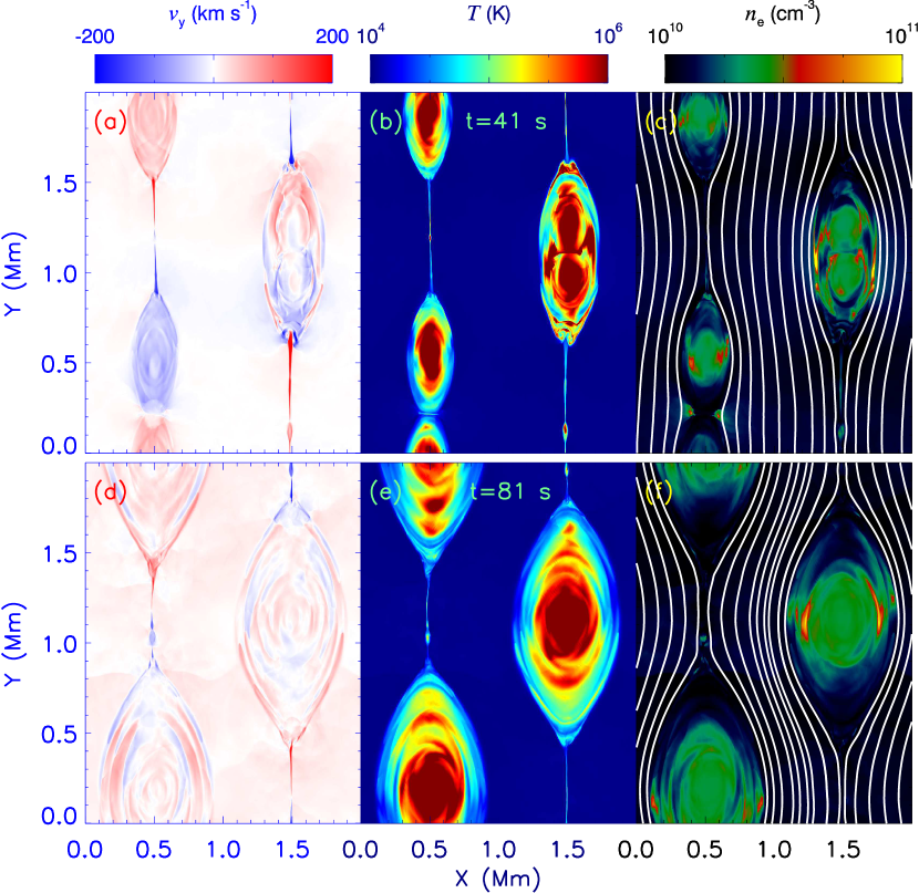
Figure 4: Similar as the upper panels of Figure 2, but at t = 41 s and t = 81 s, respectively.

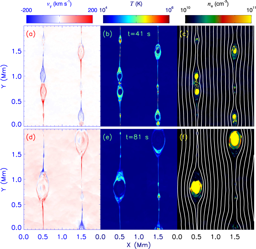
Figure 5: Similar as the bottom panels of Figure 2, but at t = 41 s and t = 81 s, respectively.

Figures 4 and 5 further display our MHD simulation results without and with the cooling process at the middle and end time of the explosive event, such as t = 41 s and t = 81 s, respectively. Their line profiles are shown in Figure 3 (c)$-$(d) and (g)$-$(h), respectively. The simulation results show that the double current sheets become broader and broader with time if there is no cooling process, and the plasma temperature in the reconnection regions are too hot to produce the line profile of Si iv 1402.77 Å, including the center and two sides of the magnetic islands. However, when we introduce the cooling function, the plasma temperature is cooling down, no matter the centers or two sides of the magnetic islands. Therefore, we can synthesize the Si iv 1402.77 Å line profiles from the 2-D MHD simulation results. Figure 3 (bottom) shows the synthetic line profiles in Si iv 1402.77 Å. It exhibits a broad non-gaussian profile (f, g and h) with a bright core and two extended (blue/red) wings (g and h).

4 Conclusions and Discussions

Using the PLUTO code, we perform a 2-D MHD simulation of the small-scale magnetic reconnection in double current sheets. Then using the simulation variables, such as the LOS velocity, number density and plasma temperature, we synthesize the line profiles of Si iv 1402.77 Å. The spectral line shows a broad non-Gaussian profile, it is complex with a bright core and two asymmetrical extended wings (blue or red shifts with velocity of nearly 200 $km~{}s^{-1}$), and this process can last for $\sim$70 s, as shown in Figure 3. All these line features agree well with the transition-region explosive events observed by IRIS (see., Innes et al., 2015). Their observations show that the spectral line profiles of Si iv 1402.77 Å at small-scale acceleration sites are broad and asymmetrical, they have bright central cores and extended blue/red wings with low intensity and fast velocity over 200 $km~{}s^{-1}$. The line emissions from the bright core and two extended wings are spatially coincident and neither move significantly during the lifetime of the explosive events. These observational line features can also be found in our simulation, as seen in the bottom panels Figure 3. Here, the double current sheet configuration is used to allow the periodic boundaries. As we know, the boundaries around the transition-region explosive events in the solar atmosphere is definitely not periodic. Thus, the periodic boundary conditions make the plasmas to flow out from one boundary and flow in from the other boundary in y-direction in this work, which has affected the reconnection region and the distributions of the plasma temperature and density. Therefore, the synthesized spectral lines will possibly be different if the other more realistic boundary conditions are applied. And we will check the simulations by using an open boundary in the future work.

The explosive evens with bi-directional jets observed in the transition regions are thought to be produced by the small-scale magnetic reconnection on the Sun (Innes et al., 1997). They have been studied by many authors based on the spectroscopic observations (e.g., Dere, 1994; Innes et al., 1997; Ning et al., 2004; Innes & Teriaca, 2013; Huang et al., 2014) and MHD simulations (Jin et al., 1996; Innes & Tóth, 1999; Sarro et al., 1999; Roussev et al., 2001). However, there is always a contradiction between the observations and the simulations of these line profiles. For example, spectroscopic observations find that the line profiles are complex with both bright cores and faint asymmetrical wings (Dere, 1994; Innes et al., 1997; Ning et al., 2004; Innes et al., 2015), while the MHD simulation results based on the Petschek model(Petschek, 1964) can only reproduce the extended wing brightening (Innes & Tóth, 1999; Biskamp, 2000; Roussev et al., 2001). This is because that the Petschek mechanism only accounts for the line wings with fast velocity, but it fails to reproduce the bright core with slow velocity since there are not enough low-speed plasmas at the diffusion region (e.g., Innes & Tóth, 1999). Recent large-scale MHD simulations show that the plasmas with fast speeds may reproduce the jets, while the plasmas with slow speeds are outside of the diffusion region (Heggland et al., 2009; Ding et al., 2011). Inspiring from that, Innes et al. (2015) present that the bright core of line profile is from the heating of the background plasmas. That is to say, the emissions from jets and backgrounds are spatially off-set, and this can result into the spatial off-sets between the line core and two extended wings brightening. This reconnection model can explain the bright core and extended wings very well. Our 2-D MHD simulations of magnetic reconnection show a rapid growth of the magnetic islands along the double current sheets. These magnetic islands are divided by the fast jets and can well explain the bright core and the extended wings of the line profiles in the explosive events. Therefore, we conclude that the transition-region explosive events with a bright core and two extended wings are most likely produced by the plasmoid instability rather than the Petschek mechanism (Petschek, 1964) during the small-scale magnetic reconnection on the Sun. The bright emission of line core is contributed from the high-density and low-velocity magnetic islands, as shown in Figures 2 (bottom) and 5.

As mentioned in Section 3.3, the key point of our 2-D MHD simulation is the cooling process. In this paper, the optically thin radiative cooling is considered, which is dependent on the cooling rates and the number density (see., equation 2). The tabulated cooling rates (see., Figure 1) are used to decrease the plasma temperature inside the reconnection region, and they seem to work well (e.g., Figures 4 and 5), especially at the temperature region between 10${}^{4}~{}K$ and 10${}^{6}~{}K$ (see also., Schmutzler & Tscharnuter, 1993; Teşileanu et al., 2008). The thermal conduction is neglected in our 2-D MHD simulation. We do not know if the heat conduction will play a role on our 2-D simulation, and it will be checked in the future work. On the other hand, we perform an initial uniform density of 10¹⁰ cm^-3 in the simulation, which can be resulted into a maximum density of $\sim$$10^{11}$ cm^-3. This value is consistent with the number density in the transition region on the Sun. Therefore, our 2-D MHD simulation conditions are very close to the situations in the solar transition region, and our simulation results agree well with the IRIS spectroscopic observations (see., Innes et al., 2015). In fact, Innes et al. (2015) have already synthesized the line profile of Si iv 1402.77 Å by using the 2-D simulation results of magnetic reconnection with plasmoid instabilities, the radiative cooling is not included in their simulations. We add the radiative cool process in our 2-D MHD simulations and obtain the similar results. In the further, we wish to work together with them using their method and code.

Innes et al. (2015) firstly successfully apply the reconnection process with plasmoid instability to explain the Si iv line profile in the transition region events. The characteristic parameters and initial conditions in their 2-D simulation have been described, i.e., the plasma density, magnetic field and temperature in the inflow regions are set to be 10¹⁰ cm^-3, 12 G, and 2$\times$10⁵ K. In our 2-D simulations, the initial plasma density, magnetic field and temperature are 10¹⁰ cm^-3, 10 G, and 2.4$\times$10⁴ K, respectively. Therefore, the initial plasma beta ($\beta$=0.02) in this work is about five times smaller than that ($\beta$=0.1) in the inflow region of Innes et al. (2015). In Innes et al. (2015), Harris Sheet is applied as the initial configurations of magnetic field (Guo et al., 2014), which makes the initial plasma density and pressure to be non-uniform across the current sheet, the initial plasma density and plasma beta in the center of the current sheet is higher than those in the inflow region. As shown in equation (3) in our simulation, the absolute value of the initial magnetic field is uniform across the current sheet, which makes the initial plasma density and pressure also to be uniform. Therefore, the different initial plasma beta ($\beta$) and initial configurations of magnetic field, plasma density and pressure are the possible reasons to cause the huge difference on the plasma heating between our work and Innes et al. (2015). The plasma in the simulation work of Innes et al. (2015) is not strongly heated as shown in our work, the maximum plasma temperature in Innes et al. (2015) only reaches the characteristic value 2$\times$10⁵ K. Therefore, the Si iv line profile can be synthesized well by using their 2-D simulation results without radiative cooling. Therefore, the radiative cooling is possibly not important in some of the transition region reconnection events.

In our 2-D simulation, the magnetic diffusion is set as a constant, and the highest resolution is (64$\times$2⁴)*(64$\times$2⁴). As we know, The resolution must be high enough in the simulations, otherwise the numerical diffusion will be higher than the magnetic diffusion set in the MHD equations and the numerical diffusion instead of the magnetic diffusion dissipate the magnetic energy. Therefore, a higher refinement level is used in our 2-D simulation, such as (64$\times$2⁵)*(64$\times$2⁵). And the simulation results by using a higher refinement level are very similar as those in our above work, i.e., the plasma temperatures both in the centers and at two sides of magnetic islands are cooling down. Therefore, the resolution in our work is high enough in our work.