Analytical properties of the gluon propagator from truncated Dyson-Schwinger equation in complex Euclidean space

Abstract

We suggest a framework based on the rainbow approximation with effective parameters adjusted to lattice data. The analytic structure of the gluon and ghost propagators of QCD in Landau gauge is analyzed by means of numerical solutions of the coupled system of truncated Dyson-Schwinger equations. We find that the gluon and ghost dressing functions are singular in complex Euclidean space with singularities as isolated pairwise conjugated poles. These poles hamper solving numerically the Bethe-Salpeter equation for glueballs as bound states of two interacting dressed gluons. Nevertheless, we argue that, by knowing the position of the poles and their residues, a reliable algorithm for numerical solving the Bethe-Salpeter equation can be established.

I Introduction

Due to the non-Abelian and confinement properties of Quantum Chromodynamics (QCD), gluons obeying self-interactions can form colorless pure gluonic bound states, also referred to as glueballs. The occurence of glueballs is one of the early predictions of the strong interactions described by QCD Jaffe . However, despite many years of experimental efforts, none of these gluonic states have been established unambiguously, cf. Ref. Jia:2016cgl . Possible reasons for this include the mixing between glueballs and ”conventional” mesons, the lack of solid information on the glueball production mechanism, and the lack of knowledge about glueball decay properties. Therefore, study of glueballs is one the most interesting and challenging problems intensively studied by theorists and experimentalists; a bulk of the running and projected experiments of the research centers, Belle (Japan), BESIII (Beijing, China), LHC (CERN), GlueX (JLAB,USA), NICA (Dubna, Russia), HIAF (China), FAIR (GSI, Germany) etc., include in the research programms comprehensive investigations of possible manifestations of glueballs. Theoretically, there are several approaches in studying glueballs. One can mention phenomenological models mimicking certain nonperturbative QCD aspects, such as the flux tube model Robson:1978iu ; Isgur:1984bm , constituent models Jaffe ; Carlson:1984wq ; Chanowitz:1982qj ; Cornwall:1982zn ; Cho:2015rsa ; Boulanger:2008aj , holographic approaches Bellantuono:2015fia ; Chen:2015zhh ; Brunner:2016ygk , approaches based on QCD Sum Rules Shifman:1978bx ; Shuryak:1982dp ; kolya ; kolya1 ; KolyaPRL . ”Experimental” studies are performed within the Lattice QCD (LQCD) approaches Albanese ; Chen ; Morningstar ; Gabadadze (for a more detailed review see Ref. Glueballstatus and references therein). It should be noted that these theoretical approaches provide values of glueball masses which can differ from each other as much as 1 GeV and even more. No single approach has consistently reproduced lattice gauge calculations, cf. Refs. Albanese ; Morningstar ; Chen ; Gabadadze . One can assert only that the consensus of the past two decades from lattice gauge theory and theoretical predictions is that the lightest glueball is a scalar ($J^{PC}=0^{++}$) state in the 1.5-1.8 GeV mass range, accompanied by a tensor ($J^{PC}=2^{++}$) state above 2 GeV.

Another interesting problem is the glueball-meson mixing in the lowest-lying scalar mesons. The question whether the lowest-lying scalar mesons are of a pure quarconium nature, or there are mixing phenomena of glueball states mixing remains still open. To solve these problems one needs to develop models within which it becomes possible to investigate, on a common footing, the glueball masses, glueball wave functions, decay modes and constants, etc. Such approaches can be based on the combined Dyson-Schwinger (DS) and Bethe-Salpeter (BS) formalisms, cf. Refs. glueBS ; GlueBallBSPRD87 . It is worth mentioning that theoretically such models, with direct calculations of the corresponding diagrams, encounter difficulties in solving the DS equation, related to divergencies of loop integrals and to the theoretical constrains on gluon-ghost and gluon-gluon vertices, such as Slavnov-Taylor identities. These circumstances result in rather cumbersome expressions for the DS equation, hindering straightforward numerical calculations.

In the present paper we suggest an approach, similar to the rainbow Dyson-Schwinger-Bethe-Salpeter model for quark propagators rob-1 , to solve the DS equation for gluon and ghost propagator with effective rainbow kernels. The formidable success of the rainbow approximation for quarks in describing mesons as quark-antiquark bound states within the framework of the BS equation with momentum dependent quark mass functions, determined directly by the DS equation, such as meson masses rob-1 ; Maris:1999nt ; Maris:2003vk ; Holl:2004fr ; Blank:2011ha , electromagnetic properties of pseudoscalar mesons Jarecke:2002xd ; Krassnigg:2004if ; Roberts:1994hh ; Roberts:2007jh ) and other observables ourFB ; wilson ; rob-2 ; Alkofer ; fisher , persuades us that the rainbow-like approximation may be successfully applied to gluons, ghosts and glueballs as well. The key property of such a framework is the self-consistency of the treatment of the quark and gluon propagators in both, DS and BS equations by employing in both cases the same approximate interaction kernel. Recall that the rainbow model for quarks consists of a replacement of the product of the coupling $g$ dressed gluon propagator ${\cal D}^{ab}_{\mu\nu}(k^{2})$ and dressed quark-gluon vertex $\Gamma_{\nu}$ by an effective running coupling and by the free vertex $\Gamma_{\nu}^{0}$ rob-1 ; rob-2 ,

$$\frac{g^{2}}{4\pi}{\cal D}_{\mu\nu}^{ab}(k^{2})\Gamma_{\nu}\to\displaystyle\frac{{\cal Z}(k^{2})}{k^{2}}D_{\mu\nu}^{free}\Gamma_{\nu}^{(0)},$$ (1)

where $a,b$ are color indices and ${\cal Z}(k^{2})$ is the effective rainbow running coupling. The explicit form of ${\cal Z}(k^{2})$ has been induced by the fact that, in the Landau gauge, it is proportional to the nonperturbative running coupling $\alpha_{s}(k^{2})$ which, in turn, is determined by the gluon $Z(k^{2})$ and ghost $G(k^{2})$ dressing functions AlkoferRunning ; Alkofer_FischerRunning ; FischerPhD ; physRep ; IRGluonProp_AlkoferSmekal ; AlkoferEstrada ; RunningCouplingAkinston ; alphaSNonpert ; IRGreen_FewBody2012 as

$$\alpha_{s}(k^{2})=\frac{g^{2}}{4\pi}G^{2}(k^{2},\mu^{2})Z(k^{2},\mu^{2}),$$ (2)

where $\mu^{2}$ is a renormalization scale parameter at $k^{2}=\mu^{2}$ whith $G^{2}(k^{2},k^{2})Z(k^{2},k^{2})=1$. In what follows, the parameter $\mu^{2}$ is suppressed in our notation and a simple notation $G(k^{2})$ and $Z(k^{2})$ is used for the dressing functions.

In principle, if one were able to solve the DS equation, the approach would not depend on any additional parameters. However, due to known technical problems, one restricts oneself to calculations of the few first terms of the perturbative series, usually within one-loop approximation, thus arriving at the truncated Dyson-Schwinger (tDS) and truncated Bethe-Salpeter (tBS) equations, known as the rainbow-ladder approximation. The merit of such an approach is that, once the effective parameters are fixed, the whole spectrum of the tBS bound states is supposed to be described without additional approximations.

In the present paper we investigate the prerequisites to the interaction kernel of the combined Dyson-Schwinger and Bethe-Salpeter formalisms to be used in subsequent calculations to describe the glueball mass spectrum. Note that within such an approach it becomes possible to theoretically investigate not only the mass spectrum of glueballs, but also different processes of their decay, which are directly connected with fundamental QCD problems (e.g., $U(1)$ axial anomaly, transition form factors etc.) and with the challenging problem of changes of hadron matter characteristics at finite temperatures and densities. All these circumstances require an adequate theoretical foundation to describe the glueball mass spectrum and their covariant wave functions (i.e. the tBS partial amplitudes) needed in calculations of the relevant Feynman diagrams and observables.

Due to the momentum dependence of the gluon and ghost dressing functions, the tBS equation requires an analytical continuation of the gluon and ghost propagators in the complex plane of Euclidean momenta which can be achieved either by corresponding numerical continuations of the solution obtained along the positive real axis or by solving directly the DS equation in the complex domain of validity of the equation itself. An analysis of the analytical properties of the propagators is of crucial importance, since if they are singular functions, the numerical calculations of corresponding integrals can be essentially hampered or even impossible in such a case. We perform a detailed analysis of the tDS equations solution by combining the Rouché’s and Cauchy’s theorems. Since the main goal of our analysis is the subsequent use of the gluon and ghost propagator functions evaluated at such complex momenta for which they are needed in the tBS equation, we focus our attention on this region of Euclidean space.

Our paper is organized as follows. In Sec. II, Subsecs. II.1 and II.2, we briefly discuss the tBS and tDS equations, relevant to describe a glueball as two-gluon bound states. The rainbow approximation for the tDS equation kernel is introduced in Subsec. II.3, and the numerical solutions of the tDS together with comparison with lattice QCD data are presented in Subsec. II.4. Section III is entirely dedicated to the solution of the tDS equation for complex Euclidean momenta, where the solutions are sought. The analytical structure of the gluon and ghost propagators in complex Euclidean space is discussed in Subsec. III.1. It is found that the ghost dressing function is analytical in the right hemisphere and contains pole-like singularities in the left hemisphere of complex momenta squared, $k^{2}$, while the gluon dressing function contains singularities in the entire Euclidean space. A thorough investigation of the pole structure of propagators is presented in Subsec. III.2. By combining Rouché’s and Cauchy’s theorems, the position of first few poles and the corresponding residues of the dressing functions are found with a good accuracy. This information is useful in elaborating adequate algorithms for numerically solving the tBS equations in presence of pole-like singularities. Conclusions and summary are collected in Sec. IV. In the Appendix A, the behaviour of the nonperturbative running coupling is discussed in connection with the choice of the rainbow kernels and a parametrization of the lattice QCD data in form of a sum of Gaussian terms is presented.

II Bethe-Salpeter and Dyson-Schwinger Equations

As mentioned above, our ultimate goal is to elaborate an effective model, based on the Dyson-Schwinger-Bethe-Salpeter approach, to describe a glueball made from two gluons that are solutions of the tDS equation for the gluon propagator. As in the rainbow approach Alkofer ; rob-1 ; rob-2 , a central requirement of our model is the self-consistent treatment of the gluon propagator in both, tBS and tDS equations. In the following we work along this strategy, i.e. we elaborate an effective model within which (i) the solution of the gluon and ghost propagators, consistent with the lattice data, is sought along the positive real axis of the momentum, (ii) then the real solution is generalized for complex momenta, relevant to the domain in Euclidean space where the tBS is defined, and (iii) an analysis, regarding the analytical properties of the complex solution, can be performed.

II.1 Bethe-Salpeter equation

We are working in Landau gauge and, consequently, we need to take into account the contribution of the Faddeev-Popov ghosts. Thus, one needs a generalization of the usual BS scheme that allows for mixing of bound states of different fields. In general, the completye system of BS equations includes also the contribution of quark-antiquark bound states, i.e. involves also glueball-meson mixing in the BS calculations. The problem of how large can be these mixing effects is not yet clearly settled. However, there are some indications, based on lattice calculations of the pure glue pseudoscalar glueball glueSpectrum , that at least in the pseudoscalar channel the glueball-meson mixing can be neglected, see also the discussion in Ref. glueBS . In what follows we will be interested in bound states for a pure gauge theory, that is neglecting quarks. The corresponding system of coupled tBS equations is presented diagrammatically in Fig. 1. The explicit form of the corresponding equations can be found, e.g. in Ref. GlueBallBSPRD87 .

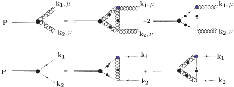
Figure 1: Diagrammatic representation of the Bethe-Salpeter equations for gluon (wiggly lines) and ghost (dashed lines) bound states. The irreducible one-particle vertices and the full propagators are represented by filled blobs.

To solve this system numerically, we need reliable information on the nonperturbative propagators of ghosts and gluons and their analytical properties in complex Euclidean momentum space. This can be achieved, e.g. by solving the tDS coupled equations for the gluon and ghost propagators along the real axis of the momentum $k$ and then to use the tDS equation at complex external momenta $k$ in Euclidean space.

II.2 Dyson-Schwinger equation

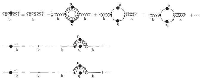
Figure 2: Diagrammatic representation of the Dyson-Schwinger equations for gluon, ghost and quark propagator. The internal wiggly, dashed and solid lines denote the full propagators represented by filled blobs. The irreducible one-particle vertices are denoted by open circles. In the gluon Dyson-Schwinger equation terms with four-gluon vertices have been dismissed.

The coupled equations of the quark, ghost and gluon propagators, and the corresponding vertex functions are often considered as integral formulation being equivalent to full QCD. While there are attempts to solve this coupled set of DS equations by sutable numerical procedures, for certain purposes some approximations and truncations fisher ; Maris:2003vk ; physRep of the exact interactions are appropriate. This leads to the truncated Dyson-Schwinger system of coupled equations for the gluon, ghost and quark propagators as depicted in Fig. 2. As mentioned above, accounting for the quark loop diagrams in the full tDS equation results in a gluon-quark mixing in the tDS equation and in a glueball-meson mixing in tBS. In most calculations such a mixing is neglected in the tBS equations. For the sake of consistency and in order to reduce the number of phenomenological parameters of the approach, the quark loops in our approach are neglected as well. This can be justified by the observation fisher ; LatticeQuenchedvsUnquenched ; QuenchedUnquenchedGluon that in the tDS equation the unquenched effects are rather small in the dynamical quark masses. As for the gluon propagator, such effects are seen only in the neighbourhood of the gluon bump, $k\sim 0.85-1.0\,{\rm GeV/c}$, where the screening effect from the creation of quark-antiquark pairs from the vacuum slightly decreases the value of the gluon dressing around its maximum. In our approach this effect is implicitly taken into account by adjusting the phenomenological parameters of the model to the full, unquenched lattice calculations GhostLatticeMishaPRD ; BornyakovLattice .

In the Landau gauge the gluon propagator ${\cal D}_{\mu\nu}^{ab}(k)$ and ghost propagator ${\cal D}_{G}^{ab}(k)$ are expressed via the dressing functions $Z(k)$ and $G(k)$ as

$${\cal D}_{\mu\nu}^{ab}(k)=-i\delta^{ab}{D}_{\mu\nu}=-i\delta^{ab}\frac{Z(k)}{k^{2}}t_{\mu\nu}(k),$$ (3)

$${\cal D}_{G}^{ab}(k)=i\delta^{ab}D_{G}(k)=i\delta^{ab}\frac{G(k)}{k^{2}},$$ (4)

where $t_{\mu\nu}(k)$ is the transverse projection operator, $t_{\mu\nu}(k)=g_{\mu\nu}-\displaystyle\frac{k_{\mu}k_{\nu}}{k^{2}}$. Then the corresponding dressing functions obey the tDS equation (cf. Fig. 2).

$$G^{-1}(k^{2}) = \tilde{Z}_{3}+\frac{3}{4\pi^{3}k^{2}}i\int d^{4}q\left[\frac{g^{2}}{4\pi}\Gamma_{\mu}^{(0)}(q)D^{\mu\nu}(p^{2})\Gamma_{\nu}(k,q,p)\right]\frac{G(q^{2})}{q^{2}},$$ (5)

$$Z^{-1}(k^{2}) = Z_{3}+\frac{i}{8\pi^{3}k^{2}}\int d^{4}q\frac{Z(q^{2})}{q^{2}}\left[\frac{g^{2}}{4\pi}\Gamma_{\mu\rho\alpha}^{(0)}(k,p,-q)D^{\rho\sigma}(p^{2})\Gamma_{\beta\sigma\nu}(q,-p,-k)\right]t^{\alpha\beta}(q)t^{\mu\nu}(k)-$$ (6)

$$- \frac{i}{4\pi^{3}k^{2}}\int d^{4}q\frac{G(q)}{q^{2}}\Gamma^{(0)}_{\mu}(q)\left[\frac{g^{2}}{4\pi}D_{G}(p^{2})\Gamma_{\nu}(p)\right]t^{\mu\nu}(k),$$

where $p=q-k$ and $Z_{3}$ and $\tilde{Z}_{3}$ are the gluon and ghost renormalization constants, respectively. To solve this system of equations one needs information about the three-gluon vertex $\Gamma_{\beta\sigma\nu}$, the gluon-ghost vertex $\Gamma_{\nu}$, the coupling $g$ and the propagators ${\cal D}_{\mu\nu}^{ab}$ and ${\cal D}_{G}^{ab}$. The simplest approach consists in a replacement of the full dressed three-gluon and ghost-gluon vertices by their bare values, known as the Mandelstam approximation CPCMandelstam ; MANDELSTAM_Approx ; PennigtonMandels and the y-max approximation YmaxApprox . In order to simplify the angular integration, in the Mandelstam approximation the gluon-ghost coupling is neglected. Then the resulting solution exhibits a rather singular gluon propagator at the origin. In Ref. YmaxApprox the coupling of the gluon to the ghost was not neglected, however additional simplifications for $Z(k^{2})$ and $G(k^{2})$ have been introduced, again to facilitate the angular integrations and the analytical and numerical analysis of the equations. From these calculations it has been concluded that it is not the gluon, but rather the ghost propagator that is highly singular in the deep infrared limit. A more rigorous analysis of the tDS equation has been presented in a series of publictions (see, e.g. Refs. IRGluonProp_AlkoferSmekal ; SmekalAnnPhys ; Fischer_Alkofer_Reinhard ; FischerPhD and references therein), where much attention has been focused on a detailed investigation of the gluon-gluon and ghost-gluon vertices and on the implementation of the Slavnov-Taylor identities for these vertices. With some additional approximations the infrared behavior of gluon and ghost propagators has been obtained analytically and compared with the available lattice calculations. In Ref. PawlowskyFicher a thorough analysis of the relevance of the Slavnov-Taylor identities, renormalization procedures and divergences in the tDS equation is presented in some details. Comparison of the numerical calculations for the gluon and ghost dressing functions and running coupling $\alpha_{s}$ with lattice data have been presented as well. Similar calculations together with a comparison with lattice data are presented also in Ref. IRGreen_FewBody2012 (for a more detailed review see Ref. FisherReview and references therein quoted). It should be noted that the above quted approaches result in rather cumbersome expressions for the system of tDS equations which, consequently, cause difficulties in finding the numerical solutions. Yet, a direct generalization to complex Euclidean space becomes problematic due to numerical problems at large $|k^{2}|$ of the complex momentum.

II.3 Rainbow approximation for ghosts and gluons

In the present paper we suggest an approximation for the interaction kernels in Eqs. (5) and (6), similar to the rainbow model Alkofer ; rob-1 ; rob-2 , Eq. (1), which allows for an analytical angular integration in the gluon and ghost loops and facilitates further numerical calculations for the complex momenta. The results of the lattice calculations of the running coupling $\alpha_{s}(k^{2})$, Eq. (2), can serve as a guideline in choosing the explicit form of these kernels. The gist of our approximations is as follows:

$$\!\!\!\!\!\!\!\!\!\!\!\!\!\!\left[\frac{g^{2}}{4\pi}\Gamma_{\mu}^{(0)}(q)D^{\mu\nu}(p^{2})\Gamma_{\nu}(k,q,p)\right]=\Gamma_{\mu}^{(0)}(q)t^{\mu\nu}(p)\Gamma_{\nu}^{(0)}(k)F^{eff}_{1}(p^{2}),$$ (7)

$$\!\!\!\!\!\!\!\!\!\!\!\!\!\!\left[\frac{g^{2}}{4\pi}\Gamma_{\mu\rho\alpha}^{(0)}(k,p,-q)D^{\rho\sigma}(p^{2})\Gamma_{\beta\sigma\nu}(q,-p,-k)\right]=A\Gamma_{\mu\rho\alpha}^{(0)}(k,p,-q)t^{\rho\sigma}(p)\Gamma_{\beta\sigma\nu}^{(0)}(q,-p,-k)F^{eff}_{1}(p^{2}),$$ (8)

$$\!\!\!\!\!\!\!\!\!\!\!\!\!\!\left[\frac{g^{2}}{4\pi}D_{G}(p^{2})\Gamma_{\nu}(p)\right]=\Gamma_{\nu}^{(0)}(p)F^{eff}_{2}(p^{2}),$$ (9)

where $A\sim 1/3$ is a phenomenological parameter which takes into account the difference in normalizations of the gluon and ghost vertices. The effective form-factors $F^{eff}_{1,2}(p^{2})$ are proportional to the infra-red part of the running coupling $\alpha_{s}(k^{2})$, see Eq. (2). The free gluon-gluon vertices $\Gamma_{\mu\rho\alpha}^{(0)}$ and $\Gamma_{\beta\sigma\nu}^{(0)}$ as well as the ghost-gluon vertices $\Gamma^{(0)}_{\mu}(q)$ and $\Gamma^{(0)}_{\nu}(q)$ read in the Landau gauge

$$\Gamma_{\mu\rho\alpha}^{(0)}(k,p,-q)=2k_{\alpha}g_{\mu\rho}+2q_{\mu}g_{\rho\alpha}-2k_{\rho}g_{\alpha\mu},$$ (10)

$$\Gamma_{\beta\sigma\nu}^{(0)}(q,-p,-k)=2q_{\nu}g_{\beta\sigma}+2k_{\beta}g_{\nu\sigma}-2k_{\sigma}g_{\beta\nu},$$ (11)

$$\Gamma^{(0)}_{\mu}(q)=-q_{\mu};\qquad\Gamma^{(0)}_{\nu}(p)=-p_{\nu}=-(q-k)_{\nu}=-q_{\nu}.$$ (12)

The rainbow approximation for the propagators in Minkowski space is obtained by inserting Eqs. (7)-(11) in to Eqs. (5) and (6) and by contracting the Lorenz indices. Further calculations are performed in Euclidean space. For this, we perform the Wick rotation of the loop integrals and specify explicitly the form of $F^{eff}_{1,2}(p^{2})$. Since we envisage the further use of the tDS equation solution in the tBS equation for bound states, where the main contribution comes from the IR region, the perturbative ultra-violet (UV) parts of $F_{1,2}^{eff}$ are neglected. Such an approximation corresponds rather to the AWW kernel Alkofer than to the full Maris-Tandy model rob-1 . As in the case of the quark rainbow approximation rob-1 ; rob-2 ; tandy1 ; wilson ; physRep , the explicit form of $F^{eff}_{1,2}(p^{2})$ is inspired by the fact that the r.h.s. of Eqs. (7)-(9) are proportional to the running coupling (2). The available QCD lattice results GhostLatticeMishaPRD show that, in the deep IR region, $\alpha_{s}$ increases as $k^{2}$ increases and reaches its maximum value at $k\sim 0.8-0.9\ {\rm GeV/c}$; then it decreases as $k^{2}$ increases and acquires the perturbative behaviour in the UV region. In Ref. GhostLatticeMishaPRD an interpolation formula consisting of three terms (monopole, dipole and quadrupole, multiplied by $k^{2}$) has been proposed to fit the data. However, we prefer an interpolation formula which, in our subsequent calculations, allows to perform angular integrations analytically and assures a good convergence of the loop integrals. For this we use a Gaussian interpolation formula and refitted the lattice data GhostLatticeMishaPRD in the IR region with several Gaussian terms and achieved a good agreement with data (see Appendix). This stimulate us to use for $F^{eff}_{1,2}(p^{2})$ the same interpolation formulae. We found that one Gaussian term for $F^{eff}_{2}(p^{2})$ and two terms for $F^{eff}_{1}(p^{2})$ are quite sufficient to obtain a reliable solution of Eqs. (5)-(6):

$$F^{eff}_{1}(p^{2})=D_{1}\frac{p^{2}}{\omega_{1}^{6}}\exp{\left(-p^{2}/\omega_{1}^{2}\right)}+D_{2}\frac{p^{2}}{\omega_{2}^{6}}\exp{\left(-p^{2}/\omega_{2}^{2}\right)},$$ (13)

$$F^{eff}_{2}(p^{2})=D_{3}\frac{p^{2}}{\omega_{3}^{6}}\exp{\left(-p^{2}/\omega_{3}^{2}\right)}..$$ (14)

With such a choice of the effective interaction, the angular integration can be carried out analytically leaving one with a system of one-dimensional integral equations in Euclidean space,

$$G^{-1}(k^{2})=\tilde{Z}_{3} - \frac{9}{8\pi}\sum_{i=1}^{2}\frac{D_{i}}{k^{2}\omega_{i}^{2}}\int G(q^{2})I_{2}^{(s)}\left(\frac{2qk}{\omega_{i}^{2}}\right){\rm e}^{-\frac{(q-k)^{2}}{\omega_{i}^{2}}}dq^{2},$$ (15)

$$Z^{-1}(k)=Z_{3} - \frac{3A}{8\pi k^{4}}\sum_{i=1}^{2}\int dq^{2}\frac{D_{i}}{\omega_{i}^{2}q^{2}}Z(q){\rm e}^{-\frac{(q-k)^{2}}{\omega_{i}^{2}}}\left\{I_{1}^{(s)}\left(\frac{2kq}{\omega_{i}^{2}}\right)\left[\phantom{\!\!\!\!\!\frac{1}{2}}-12k^{3}q-12kq^{3}-5kr\omega_{i}^{2}\right]\right.$$ (16)

$$+ \left.I_{2}^{(s)}\left(\frac{2kq}{\omega_{i}^{2}}\right)\left[\phantom{\!\!\!\!\frac{1}{2}}6k^{4}+6q^{4}+10\omega_{i}^{4}+18k^{2}q^{2}+24k^{2}\omega_{i}^{2}+24q^{2}\omega_{i}^{2}\right]\right\}$$

$$+ \frac{3D_{3}}{8\pi k^{4}}\int dq^{2}G(q){\rm e}^{-\frac{(q-k)^{2}}{\omega_{3}^{2}}}I_{2}^{(s)}\left(\frac{2kq}{\omega_{3}^{2}}\right),$$

where $I_{n}^{(s)}(x)$, with $x\equiv\displaystyle\frac{2kq}{\omega^{2}}$, are the scaled (as emphasized by the label ”(s)”) modified Bessel functions of the first kind defined as $I_{n}^{(s)}(x)\equiv\exp{(-x)}\ I_{n}(x)$.

II.4 Numerical solution along the real axis

The resulting system of one-dimensional integral equations (15) and (16) we solve numerically by an iteration procedure. For this we discretize the loop integrals by using the Gaussian integration formula, so that the system of integral equations reduces to a system of algebraic equations. Independent parameters are $\omega_{i}$ and $D_{i}$, $i=1\cdots 3$, see Eqs. (13), (14). We find that the iteration procedure converges rather fast and practically does not depend on the choice of the trial start functions. The phenomenological parameters $\omega_{i}$ and $D_{i}$ have been adjusted in such a way as to reproduce as close as possible the lattice QCD results GhostLatticeMishaPRD ; BornyakovLattice .

Few remarks are in order here. First, the deep infrared behaviour of the ghost and gluon propagators requires a separate consideration. It has been established that the gluon dressing $Z(k^{2})$ vanishes at the origin, while the ghost $G(k^{2})$ is highly singular, see e.g. Refs. AlkoferRunning ; IRGluonProp_AlkoferSmekal ; SmekalAnnPhys ; IRGreen_FewBody2012 . In the deep IR region, $k\leq\epsilon$ the gluon and ghost dressing are predicted to behave as

$$Z(k^{2}\leq\epsilon^{2})\sim(k^{2})^{2\kappa};\quad G(k^{2}\leq\epsilon^{2})\sim(k^{2})^{-\kappa},$$ (17)

where $\kappa$ varies in the interval $\kappa\simeq 0.45-0.92$ and $\epsilon\sim 0.1-1.0$ MeV/c. In this region, we force ”by hand” the ghost and gluon propagator to follow Eq. (17), i.e. they do not change during the iteration procedure. In other words, the iteration starts at $k>\epsilon$. We choose $\kappa=0.45$ and $\epsilon=0.1$ MeV. Since $\epsilon$ is extremely small, the constrains in Eq. (17) do not affect the loop integrations and they are not substantial at all in our further calculations. Second, the Gaussian form of the interaction kernels (13)-(14) assures a good convergence of the iteration procedure. In principle, it suffices to employ a relatively small mesh ($48-64$ Gaussian nodes) to find a stable solution of Eqs. (15)-(16). However, in the subsequent calculations of the propagators in complex plane, the tDS equation solution along the real axis $q$ is used for complex values of $k^{2}$ for which the integrands become highly oscillating functions at large values of Im $k^{2}$. To assure a good accuracy of numerical calculations in this case one needs to have the solution of the tDS equation along the real axis in a sufficiently dense Gaussian mesh. For this sake, the whole interval $q=[0..q_{max}]$ is divided in to three parts: (i) $[0\leq q\leq\epsilon]$ with 16 Gaussian nodes. In this interval the ghost and gluon dressing functions are taken in accordance with Eqs. (17), (ii) $[\epsilon\leq q\leq 1.1{\rm~{}GeV/c}]$ is the interval around the maximum of the gluon propagator. Here the Gaussian mesh is taken to consist on 156 nodes, (iii) in the remaining interval $[1.1{\rm~{}GeV/c}\leq q\leq q_{max}]$ the Gaussian mesh with 120-156 nodes is used. The maximum value $q_{max}$ is chosen so that the integrands (15)-(16) are independent of $q_{max}$. In our case, the value $q_{max}=5$ GeV/c is sufficient to assure a good accuracy of the solution. By iterating Eqs. (15)-(16), we fit the parameters $D_{i}$ and $\omega_{i}$ of the kernels (13)-(14) to obtain a reliable agreement with the lattice QCD results  GhostLatticeMishaPRD ; BornyakovLattice . The renormalization constants $\tilde{Z}_{3}$ and $Z_{3}$ are defined at the renormalization point $\mu=2.56$ GeV and $\mu=3.0$ GeV respectively. With the set of parameters $D_{1}=1.128\ {\rm GeV^{2}/c^{2}}$, $D_{2}=0.314\ {\rm GeV^{2}/c^{2}}$, $D_{3}=95\ {\rm GeV^{2}/c^{2}}$, $\omega_{1}=0.7\ {\rm GeV/c}$, $\omega_{2}=2.16\ {\rm GeV/c}$ and $\omega_{3}=0.55\ {\rm GeV/c}$ the renormalization constants are found to be $\tilde{Z}_{3}=1.065$ and $Z_{3}=1.05$. The corresponding solution for the ghost and gluon propagators are presented in Fig. 3.

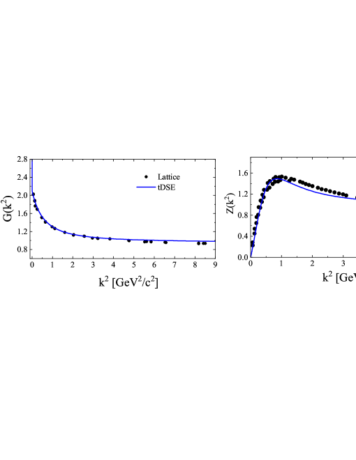
Figure 3: (Color online) Solution of the tDS equations (15)-(16) (solid lines) in comparison with lattice calculations BornyakovLattice ; GhostLatticeMishaPRD (filled circles). Left panel: ghost dressing function, right panel: gluon dressing function.

It is seen that both, ghost and gluon dressings are smooth, positively defined functions not containing any singularity, except for the ghost dressing, which according to Eq. (17), is singular at the origin. One can conclude that, with the chosen set of parameters, the solution of the tDS equation satisfactorily describes the lattice data. This encourages us to use the tDS equation along the real $q$ to find solutions for complex $k$, treating it as external parameter in the tDS equation.

III Solutions of the tDS equation in complex plane

The solution of the tDS equation along the positive real axis of momenta is generalized to complex values of $k^{2}$, needed to solve the tBS equation for bound states. The tBS equation is defined in a restricted complex domain of Euclidean space, which is determined by the propagators of the constituents. Usually this momentum region is displayed as the dependence of the imaginary part of the constituent gluon momentum squared, Im $k^{2}$, on its real part, Re $k^{2}$, determined by the tBS equation. In terms of the relative momentum $k_{rel}$ of the two dressed gluons residing in a glueball, the corresponding dependence is

$$k^{2}=-\displaystyle\frac{M_{gg}^{2}}{4}+k_{rel}^{2}\pm iM_{gg}k_{rel}$$ (18)

determining in the Euclidean complex momentum plane a parabola  Im $k^{2}=\pm~{}M_{gg}\sqrt{{\rm Re}\,k^{2}~{}+~{}\frac{M_{gg}^{2}}{4}}$ with vertex at Im $k^{2}=0$ at Re $k^{2}=-M_{gg}^{2}/4$ depending on the glueball mass $M_{gg}$. The symmetry axis is the Re $k^{2}$ axis, i.e. the parabola extends to Re $k^{2}\to\infty$.

It should be noted that, for the quark-antiquark bound states the use of the complex rainbow solution in to the tBS equation provides an amazingly good description of many properties of light mesons (masses, widths, decay rates etc., cf. Maris:2003vk ; Holl:2004fr ; Jarecke:2002xd ; Krassnigg:2004if ; Roberts:1994hh ; Maris:2000sk ; Maris:1999bh ; ourFB ). However, for heavier mesons the quark propagators possess pole-like singularities OurAnalytical ; dorkinBSmesons which hamper the numerical procedure in solving the tBS equation. An analogous situation can appear for the complex solution of the gluon and ghost propagators. Hence, a more detailed investigation of the gluon dressing functions in the complex Euclidean plane is required. There are some considerations, based on studies of the gauge fixing problem, according to which the gluon propagator contains complex conjugate poles in the negative half-plane of squared complex momenta $k^{2}$ ZwangerANalit ; Stingl ; CucchieriAnalit . The knowledge of the nature of singularities and their exact location in the complex plane is of a great importance since it will allow one to develop effective algorithms adequate for numerical calculations. For instance, if one determines exactly the domain of analyticity of the propagator functions, one can take advantage of the fact that any analytical function can always be approximated by rational complex functions walsh ; then, one can parametrize the integrand in the tBS equation by simple functions which allow ones to carry out some integrations analytically.

There are several possible procedures (cf. Refs. analiticalFischer ; GluonAnalyticalFisherPRL2012 ) of how to obtain a complex solution of the tDS equations once the equation has been solved for real and spacelike Euclidean momenta. First, one can use the so-called shell method. This method acknowledges the fact that for fixed external momentum $k^{2}$ the relative momentum $(p-q)^{2}$ samples only a parabolic domain in the complex momentum plane. Therefore, one starts with a sample of external momenta on the boundary of a typical domain very close to the real positive momentum axis. The tDS equations are then solved on this boundary, while the interior points are obtained by interpolation. In the next step, a slightly larger parabolic domain is used, with points in the interior given by the previous solution. This way one extends the solution of the tDS equations step by step further away from the Euclidean result into the whole complex plane. A shortcoming of the method is that there is an accumulation of numerical errors at each step of the calculations.

A second option is to deform the loop integration path itself away from the real positive $k^{2}$ axis MarisComplexDSE ; OurAnalytical . This can be done by deforming the integration contour and solving the integral equation along this new contour. For complex momenta $k$, one has to solve the integral equation along a deformed contour in the complex plane. In practice, one changes the integration contour by rotating it in the complex plane, multiplying both the internal and the external variable by a phase factor $e^{i\phi}$, so one gets the complex variables $k=|k|e^{i\phi}$ and $q=|q|e^{i\phi}$ and solves the tDS equation along the rays $\phi=const$. This method works quite well in the first quadrant, $\phi\leq\pi/2$, but fails at $\phi>\pi/2$, see e.g. Ref. OurAnalytical ; dorkinBSmesons . This is because along the rays $\phi=const$ all the values of $|k|$, from $|k|=0$ to $|k|\to\infty$ contribute to the tDS equation, even if one needs the solution only in a restricted area of the parabola Im $k^{2}<0$. Consequently, numerical instabilities are inevitable at $\phi>\pi/2$.

The third method, which we use in this work, consists in finding a solution to the integral equations in a straightforward way from the tDS equation along the real $q$ on a complex grid for the external momentum $k$ inside and in the neighbourhood of the parabola (18). As in the previous case, numerical instabilities can be caused by oscillations of the exponent ${\rm e}^{-(k-q)^{2}/\omega^{2}}$ and of the Bessel functions $I_{1,2}^{(s)}(2kq/\omega^{2})$ at large $|k^{2}|$. However, one can get rid of such a numerical problem by taking into account that parabola (18) restricts only a small portion of the complex plane at Re $k^{2}<0$, where the numerical problems are minimized. For positive values of Re $k^{2}>0$, where $|k^{2}|$ can be large, the tBS wave function of a glueball is expected to decrease rapidly with increasing argument $k_{rel}$, and at $k_{rel}^{max}\sim 3-4\ {\rm GeV/c}$ to become negligibly small. So, one can solve the complex tDS equation at not too large $|k^{2}|$, where a reliable calculation of the loop integrals in Eqs. (15)-(16) is still possible. Then one takes advantage of the fact that, at larger values of $k_{rel}$, the highly oscillating integrals in (15)-(16) are negligible small or even vanish at $k_{rel}\to\infty$, in accordance with the Riemann-Lebesgue lemma. Consequently, such integrals can be safely neglected. This means that it suffices to investigate the behaviour of the gluon and ghost propagators for a parabola with $k_{rel}^{max}\sim 3-4\ {\rm GeV/c}$. In what follows we analyze the analytical properties of the dressing functions $Z(k)$ and $G(k)$ in the complex domain of parabola from $Rek^{2}$ corresponding to glueball masses $M_{gg}\leq 5\,{\rm GeV/c^{2}}$ up to Re $k^{2}$ corresponding to $k_{rel}^{max}\sim 3.5\ {\rm GeV/c}$.

III.1 Analytical structure of the gluon and ghost propagators in complex Euclidean space

To determine the analytical properties of $Z(k)$ and $G(k)$ we use a combined method dorkinBSmesons ; OurAnalytical based on calculations of the Cauchy and Rushe integrals. In a closed domain, the Cauchy integral of an analytical function $f(z)$ vanishes. Contrarily, the non-zero Cauchy integral undoubtedly indicates that $f(z)$ is singular inside the domain. In this case, to locate and investigate the nature of the singularities one computes the Cauchy integral of the inverse function $g(z)=1/f(z)$. The vanishing Cauchy integral of the inverse function means that $g(z)$ is analytical in the considered domain. Consequently, one concludes that the singularities of $f(z)$ can be solely of the pole-type. Evidently, the positions of such poles coincide with the positions of the zeros of $g$. The zeros of $g$ can be found by the Rushe theorem , according to which the Rouché integral must be an integer, exactly equal to the number of zeros inside the domain. Our calculations show that both, Cauchy integral of $G(k^{2})$ and Cauchy integral of $Z(k^{2})$, are different from zero, i.e. $G(k^{2})$ and $Z(k^{2})$ are singular inside the parabola. Then, the further strategy of finding these singularities is as follows:
(i) Consider consecutively the dressing functions $G(k^{2})$ and $Z(k^{2})$. Choose a contour inside the parabola and compute the Cauchy integral of $G(k^{2})$ (or $Z(k^{2})$). If the integral is zero, we choose another contour nearby the previous one and repeat the calculations until a non-zero integral is encountered. Check whether the singularities here are of pole-type, i.e. compute the Cauchy integral of the inverse, $G(k^{2})^{-1}$ (or $Z(k^{2})^{-1}$), which must be zero if singularities are isolated poles.
(ii) Compute the Rouché integral of $G(k^{2})^{-1}$ (or $Z(k^{2})^{-1}$). Since the inverse function has been found to be analytical, such an integral, according to the Rouché’s theorem, gives exactly the number of zeros inside the contour.
(iii) Squeeze the contour and repeat items (i)-(ii), keeping the zero inside, until an isolated zero of $G(k^{2})^{-1}$ (or $Z(k^{2})^{-1}$) is located with a desired accuracy. The corresponding integrals around such isolated poles $k_{0i}^{2}$ read as

$$\frac{1}{2\pi i}\oint\limits_{\gamma}\left[G(k^{2})\left(Z(k^{2})\right)\right]dk^{2}=\sum_{i}res\left[G(k_{0i}^{2})\left(Z(k_{0i}^{2})\right)\right],$$ (19)

$$\frac{1}{2\pi i}\oint\limits_{\gamma}G^{-1}(k^{2})\left(Z^{-1}(k^{2})\right)dk^{2}=0.$$ (20)

$$\frac{1}{2\pi i}\oint\limits_{\gamma}\frac{\left[G^{-1}(k^{2})\left(Z^{-1}(k^{2})\right)\right]^{\prime}_{k^{2}}}{G^{-1}(k^{2})\left(Z^{-1}(k^{2})\right)}dk^{2}=N_{G(Z)},$$ (21)

where $N_{G(Z)}$ is the number of poles in the domain enclosed by the contour $\gamma$ (an effective algorithm for numerical evaluations of Cauchy-like integrals can be found, e.g. in Ref. ioak ). In such a way we find the poles of $G(k^{2})$ and $Z(k^{2})$ together with their residues relevant for further calculations. In subsequent numerical calculations of integrals, involving functions with pole-like singularities, one can use the following theorem: if a complex function $f(z)$ possesses isolated poles, then it can be represented in the form

$$f(z)=\widetilde{f}(z)+\sum_{i}\frac{{\rm res}[f(z_{0i})]}{z-z_{0i}},$$ (22)

where $\widetilde{f}(z)$ is analytical within the considered domain and, consequently, can be computed as

$$\widetilde{f}(z)=\frac{1}{2\pi i}\oint\limits_{\gamma}\frac{\widetilde{f}(\xi)}{\xi-z}d\xi=\frac{1}{2\pi i}\oint\limits_{\gamma}\frac{f(\xi)}{\xi-z}d\xi.$$ (23)

Note that a good numerical test of the performed calculations is the following procedure. Enclose a few poles by a larger contour and ensure that the Cauchy integral of $G(k^{2})$ or $Z(k^{2})$ is different from zero and that the Rouché integral of the inverse, $G(k^{2})^{-1}$ or $Z(k^{2})^{-1}$, is an integer equal to the number of enclosed poles. Note that the Cauchy integral of $G(k^{2})$ or $Z(k^{2})$ in this case must coincide with the sum of individual residues of the isolated poles.

III.2 Pole structure of the dressing functions

Table 1: The pole structure of the gluon, $Z(k^{2})$, and ghost, $G(k^{2})$, dressing functions. The pole positions $(Re\ k_{0}^{2},Im\ k_{0}^{2})$ and the corresponding residues are in units of ${\rm(GeV/c)}^{2}$. Only the first, four self-conjugated poles on $k^{2}$ close to the parabolas (18), see also Fig. 4, are presented.

Gluons	1	2	3	4
$k_{0i}^{2}$	(-3.52, $\pm$ 6.97)	(-1.975, $\pm$ 2.05)	(-0.605,$\pm$ 6.02)	(0.11,$\pm$ 0.61)
res[$Z(k_{0i}^{2}$ ]	(-0.0536, $\mp$ 0.01755)	(0.051,$\mp$ 0.081)	(0.79, $\mp$ 0.079)	(0.589,$\pm$ 0.0791)
Ghosts	1	2	3	4
$k_{0i}^{2}$	(-2.47, $\pm$ 7.37)	(-1.915,$\pm$ 4.15)	(-0.687, 0.0)	–
res[$G(k_{0i}^{2}$ ]	(0.4667 $\pm$ 0.036)	(0.494, $\pm$ 0.082)	(0.956,$\mp$ 0.0)	–

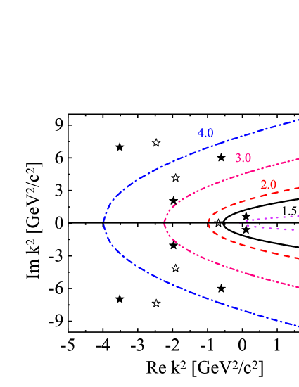
Figure 4: (Color online) Positions of few first poles of the gluon $Z(k^{2})$, full stars, and ghost, $G(k^{2})$, open stars, dressing function in the complex $k^{2}$ plane, labeled in correspondence to the Table 1. The relevant sections of the parabola (18) corresponding to the glueball bound-state mass $M_{gg}$ are presented for $M_{gg}=0.5,\,1.5,\,2,\,3$ and $4$ GeV, from right to left. The tendency is that, with increasing glueball bound-state mass $M_{gg}$, more and more poles are located in the physical area, relevant to the tBS equation.

Results of our calculations are presented in Table 1 and Fig. 4. It is seen that for $M_{gg}<5\,{\rm GeV/c^{2}}$ all singularities of the gluon dressing $Z(k^{2})$ are pairwise complex conjugated. There are two complex conjugated poles at Re $k^{2}>0$ which means that a glueball bound state contains at least two poles, regardless the glueball mass $M_{gg}$, except for very low values of $M_{gg}<0.5\ {\rm GeV}$, see Fig. 4. Contrarily, all singularities of the ghosts are located in the region $Re\ k^{2}<0$ with one real pole at Re $k^{2}\approx-0.69\ {\rm GeV^{2}/c^{2}}$.

Results of calculations by Eqs. (19)-(21) provide all the necessary ingredients for Eqs. (22)-(23,) allowing to establish easily reliable algorithms for solving numerically the tBS equation even in the presence of pole-like singularities.

With these calculations our analysis of the pole structure is completed. Let us recall the prepositions: (i) The tDS equation is solved in an approach similar to the rainbow approximation with IR part only. The phenomenological parameters have been adjusted to lattice QCD results. (ii) The tDS equation, restricted to the momentum range relevant for $gg$ bound states, $M_{gg}<5\,{\rm GeV/c^{2}}$.

IV Summary

We analyse analytical properties of solutions of the truncated Dyson-Schwinger equation for the ghost and gluon propagators in the Euclidean complex momentum domain which is determined by the truncated Bethe-Salpeter equation for two-gluon bound states. Our approach is based on an approximation, similar to the rainbow approach for quarks, with effective parameters adjusted in accordance with the available lattice QCD data. It is found that, within the suggested approach with only the infrared terms in the combined effective vertex-gluon dressing and vertex-ghost dressing kernels, the solutions $Z(k^{2})$ and $G(k^{2})$ are singular in the whole considered domain for $M_{gg}<5\,{\rm GeV/c^{2}}$, with singularities as isolated pairwise complex conjugated poles. The exact position of the poles and the corresponding residues of the propagators can be found by applying Rouché theorem and computing the Cauchy integrals.

The position of the few first poles and the corresponding residues are found with good accuracy to be used in further calculations based on the Bethe-Salpeter equation. It is also found that, with only the effective infrared term in the parametrization of the combined vertex-gluon and vertex-ghost kernels, the ghost dressing function exhibits a pole on the negative real axis. The performed analysis is aimed at elaborating adequate numerical algorithms to solve the truncated Bethe-Salpeter equation in presence of singularities and to investigate the properties of glueballs, e.g. scalar and pseudoscalar glueball states.

Appendix A

The model interaction kernels in the rainbow approximations is inspired essentially by the behaviour of the running coupling (2) in the IR region, which now is available from the lattice QCD data GhostLatticeMishaPRD . In order to facilitate the calculations, the explicit expressions for the kernels are taken in form of Gaussian terms. Accordingly, it is preferably to have the parametrization of the running coupling also in such a form. Usually, in original publications of the lattice QCD results one employs parametrizations to fit data as a sum of several multipole terms, cf. GhostLatticeMishaPRD ; BornyakovLattice . For our purpose we have to refit the data within another, Gaussian-like formula. Here below we present a fit for the running coupling (2) in form of a sum of several Gaussian terms with fitting parameters found from a Levenberg minimization procedure. Such a parametrization serves as a guideline in choosing the form of the effective kernels (13)-(14).

$$\alpha_{s}(p^{2})=p^{2}\sum_{i=1}^{5}A_{i}{\rm e}^{-a_{i}p^{2}}.$$ (24)

The minimization procedure converged to a set of parameters listed in Table 2, which provide a fit of lattice QCD data presented in Fig. 5.

Table 2: The parameters $A_{i}$ and $a_{i}$ (in $[{\rm\left(GeV/c\right)^{-2}}]$) for the effective parametrizations, Eq. (24), of the lattice QCD results GhostLatticeMishaPRD .

		1		2		3		4		5
$A_{i}$		4.546		0.840		0.146		2.472		6.87
$a_{i}$		1.804		0.636		0.196		3.45		4.51

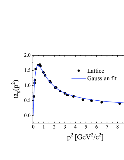
Figure 5: (Color online) The fit of the nonperturbative running coupling $\alpha_{s}(p)$ by Eq. (24) (solid line) vs. the results of lattice QCD calculations GhostLatticeMishaPRD (filled circles).

References

- (1) R. L. Jaffe and K. Johnson, Unconventional States of Confined Quarks and Gluons, Phys. Lett. B 60, 201 (1976).
- (2) S. Jia et al. (The Belle Collaboration), Search for the Glueball in and decays, Phys. Rev. D 95, 012001 (2017).
- (3) D. Robson, Toroidal Bags (where To Stick Your Gluons), Z. Phys. C 3 , 199 (1980).
- (4) N. Isgur and J. E. Paton, A Flux Tube Model for Hadrons in QCD, Phys. Rev. D 31, 2910 (1985).
- (5) C. E. Carlson, T. H. Hansson, and C. Peterson, The Glueball Spectrum in the Bag Model and in Lattice Gauge Theories, Phys. Rev. D 30 , 1594 (1984).
- (6) M. S. Chanowitz and S. R. Sharpe, Hybrids: Mixed States of Quarks and Gluons, Nucl. Phys. B 222, 211 (1983) [Erratum Nucl. Phys. B 228, 588 (1983)].
- (7) J. M. Cornwall and A. Soni, Glueballs as Bound States of Massive Gluons, Phys. Lett. B 120, 431 (1983).
- (8) Y. M. Cho, X.Y. Pham, P. Zhang, J.-J. Xie et al., Glueball Physics in QCD, Phys. Rev. D 91, 114020 (2015).
- (9) N. Boulanger, F. Buisseret, V. Mathieu, and C. Semay, Constituent gluon interpretation of glueballs and gluelumps, Eur. Phys. J. A 38, 317 (2008).
- (10) L. Bellantuono, P. Colangelo, and F. Giannuzzi, Holographic Oddballs, JHEP 10, 137 (2015).
- (11) Y. Chen and M. Huang, Two-gluon and trigluon, glueballs from dynamical holography QCD, Chin. Phys. C 40 , 123101 (2016).
- (12) F. Brunner and A. Rebhan, Holographic QCD predictions for production and decay of pseudoscalar glueballs, Phys. Lett. B 770, 124 (2017).
- (13) M. A. Shifman, A. I. Vainshtein, and V. I. Zakharov, QCD and Resonance Physics. Theoretical Foundations, Nucl. Phys. B 147, 385 (1979).
- (14) E. V. Shuryak, The Role of Instantons in Quantum Chromodynamics. 2. Hadronic Structure, Nucl. Phys. B203, 116 (1982).
- (15) A. Pimikov, H.-J. Lee, N. Kochelev, P. Zhang and V. Khandramai, Exotic glueball states in QCD sum rules, Phys. Rev. D 96, 114024 (2017).
- (16) A. Pimikov, H.-J. Lee, N. Kochelev, Comment on ”Finding the Glueball”, Phys. Rev. Lett. 119,079101 (2017).
- (17) A. Pimikov, H.-J. Lee, N. Kochelev and P. Zhang, Is the exotic glueball a pure gluon state?, Phys. Rev. D 95, 071501 (2017).
- (18) M. Albanese et al. [Ape Collaboration], Glueball Masses and the Loop Loop Correlation Functions, Phys. Lett. B 197, 400 (1987).
- (19) Y. Chen, A. Alexandru, S. Dong, T. Draper, I. Horvath et al. Glueball spectrum and matrix elements on anisotropic lattices, Phys. Rev. D 73, 014516 (2006).
- (20) C. J. Morningstar and M. J. Peardon, The Glueball spectrum from an anisotropic lattice study, Phys. Rev. D 60, 034509 (1999).
- (21) G. Gabadadze, Pseudoscalar glueball mass: QCD versus lattice gauge theory prediction, Phys. Rev. D 58, 055003 (1998).
- (22) W. Ochs, The Status of Glueballs, J. Phys. G 40, 043001 (2013).
- (23) H. Noshad, S. M. Zebarjad and S. Zarepour, Mixing among lowest-lying scalar mesons and scalar glueball, Nucl. Phys. B 934, 408 (2018).
- (24) H. Sanchis-Alepuz, C. S. Fischer, C. Kellermann and L. von Smekal, Glueballs from the Bethe-Salpeter equation, Phys. Rev. D 92, 034001 (2015).
- (25) J. Meyers and E. S. Swanson, Spin Zero Glueballs in the Bethe-Salpeter Formalism, Phys. Rev. D 87, 036009 (2013).
- (26) P. Maris and C. D. Roberts, pi- and K meson Bethe-Salpeter amplitudes, Phys. Rev. C 56, 3369 (1997).
- (27) P. Maris and P. C. Tandy, Bethe-Salpeter study of vector meson masses and decay constants, Phys. Rev. C 60, 055214 (1999).
- (28) P. Maris and C.D. Roberts, Dyson-Schwinger equations: A tool for hadron physics, Int. J. Mod. Phys. E 12, 297 (2003).
- (29) A. Holl, A. Krassnigg and C.D. Roberts, Pseudoscalar meson radial excitations, Phys. Rev. C 70, 042203 (2004).
-
(30)
M. Blank and A. Krassnigg,
Bottomonium in a Bethe-Salpeter-equation study,
Phys. Rev. D 84, 096014 (2011);
M. Blank, A. Krassnigg and A. Maas, rho-meson, Bethe-Salpeter equation, and the far infrared, Phys. Rev. D 83, 034020 (2011). - (31) D. Jarecke, P. Maris and P. C. Tandy, Strong decays of light vector mesons, Phys. Rev. C 67, 035202 (2003).
- (32) A. Krassnigg and P. Maris, Pseudoscalar and vector mesons as q anti-q bound states, J. Phys. Conf. Ser. 9, 153 (2005).
- (33) C. D. Roberts, Electromagnetic pion form-factor and neutral pion decay width, Nucl. Phys. A 605, 475 (1996).
- (34) C. D. Roberts, M. S. Bhagwat, A. Holl and S. V. Wright, Aspects of hadron physics, Eur. Phys. J. ST 140, 53 (2007).
- (35) S. M. Dorkin, T. Hilger, L. P. Kaptari and B. Kämpfer, Heavy pseudoscalar mesons in a Dyson-Schwinger–Bethe-Salpeter approach, Few Body Syst. 49, 247 (2011).
-
(36)
S. -x. Qin, L. Chang, Y. -x. Liu, C. D. Roberts and D. J. Wilson,
Interaction model for the gap equation,
Phys. Rev. C 84, 042202 (2011);
S. -x. Qin, L. Chang, Y. -x. Liu, C. D. Roberts and D. J. Wilson, Investigation of rainbow-ladder truncation for excited and exotic mesons, Phys. Rev. C 85, 035202 (2012). - (37) M. R. Frank and C. D. Roberts, Model gluon propagator and pion and rho meson observables, Phys. Rev. C 53, 390 (1996).
- (38) R. Alkofer, P. Watson and H. Weigel, Mesons in a Poicare BS approach, Phys. Rev. D 65, 094026 (2002).
- (39) C. S. Fischer, P. Watson and W. Cassing, Probing unquenching effects in the gluon polarisation in light mesons, Phys. Rev. D 72 ,094025 (2005).
- (40) C. S. Fischer and R. Alkofer, Infrared Exponents and Running Coupling of SU(N) Yang–Mills Theories, Phys. Lett. B 536, 177 (2002).
- (41) C. S. Fischer and R. Alkofer, Non-perturbative Propagators, Running Coupling and Dynamical Quark Mass of Landau gauge QCD, Phys. Rev. D 67, 094020 (2003).
- (42) C. S. Fischer, Non-perturbative Propagators, Running Coupling and Dynamical Mass Generation in Ghost-Antighost Symmetric Gauges in QCD, e-Print: hep-ph/0304233 (PhD-thesis, Univ. of Tuebingen. Nov 2002).
- (43) R. Alkofer and L. von Smekal, The Infrared behavior of QCD Green’s functions: Confinement dynamical symmetry breaking, and hadrons as relativistic bound states, Phys. Rept. 353, 281 (2001).
- (44) L. von Smekal, A. Hauck and R. Alkofer, The Infrared Behavior of Gluon and Ghost Propagators in Landau Gauge QCD, Phys. Rev. Lett. 79, 3591 (1997).
- (45) R. Alkofer, C. S. Fischer and F. J. Llanes-Estrada, Vertex functions and infrared fixed point in Landau gauge SU(N) Yang-Mills theory, Phys.Lett. B 611, 279 (2005), Erratum: Phys. Lett. B 670, 460 (2009).
- (46) D. Atkinson and J.C.R. Bloch, Running Coupling in Non-Perturbative QCD, Phys Rev. D 58, 094036 (1998).
- (47) G. Bergner and S. Piemonte, The running coupling from gluon and ghost propagators in the Landau gauge: Yang-Mills theories with adjoint fermions, Phys. Rev. D 97, 074510 (2018).
- (48) Ph. Boucaud, J. P. Leroy, A. Le Yaouanc, J. Micheli, O. Pene and J. Rodriguez-Quintero, The Infrared Behaviour of the Pure Yang-Mills Green Functions, Few-Body Syst. 53, 387 (2012).
- (49) Y. Chen, A. Alexandru, S.J. Dong, T. Draper, I. Horvath et al., Glueball spectrum and matrix elements on anisotropic lattices, Phys.Rev. D 73, 014516 2006).
- (50) P. O. Bowman, U. M. Heller, D. B. Leinweber, M. B. Parappilly, A. Sternbeck, L. von Smekal, A. G. Williams and J. Zhang, Scaling behavior and positivity violation of the gluon propagator in full QCD, Phys. Rev. D 76, 094505 (2007).
- (51) P. O. Bowman, U. M. Heller, D. B. Leinweber, M.B. Parappilly amd A. G. Williams, Unquenched Gluon Propagator in Landau Gauge, Phys. Rev. D 70, 034509 (2004).
- (52) V. G. Bornyakov, E.-M. Ilgenfritz, C. Litwinski, M. Müller-Preussker and V. K. Mitrjushkin, Landau gauge ghost propagator and running coupling in SU(2) lattice gauge theory, Phys. Rev. D 92, 074505 (2015).
- (53) V. G. Bornyakov, V. K. Mitrjushkin and M. Müller-Preussker, SU(2) lattice gluon propagator: continuum limit, finite-volume effects and infrared mass scale , Phys. Rev. D81, 054503 (2010).
- (54) A. Hauck, L. von Smekal and R. Alkofer, Solving the Gluon Dyson-Schwinger Equation in the Mandelstam Approximation, Comput. Phys. Commun. 112, 149 (1998).
- (55) S. Mandelstam, Approximation scheme for quantum chromodynamics, Phys. Rev. D 20, 3223 (1979).
- (56) Kirsten Buttner and M.R. Pennington, Infrared behavior of the gluon propagator: Confining of confined? Phys. Rev. D 52, 5220 (1995).
- (57) D. Atkinson and J. C. R. Bloch, Running coupling in nonperturbative QCD. 1. Bare vertices and y-max approximation, Phys. Rev. D 58, 094036 (1998).
- (58) L. von Smekal, A. Hauck and R. Alkofer, A Solution to Coupled Dyson–Schwinger Equations for Gluons and Ghosts in Landau Gauge, Ann. Phys. 267, 1 (1998), Erratum: Ann. Phys. 269, 282 (1998).
- (59) C. S. Fischer, R. Alkofer and H. Reinhardt, The Elusiveness of Infrared Critical Exponents in Landau Gauge Yang-Mills Theories, Phys. Rev. D 65, 094008(2002).
- (60) C. S. Fischer, A. Maas and J. M. Pawlowski, On the infrared behavior of Landau gauge Yang-Mills theory, Ann. Phys. 324, 2408 (2009).
- (61) C. S. Fischer, Infrared Properties of QCD from Dyson-Schwinger equations, J. Phys. G 32, R253 (2006).
- (62) P. Tandy, Hadron physics from the global color model of QCD, Prog. Part. Nucl. Phys. 39, 117 (1997).
- (63) P. Maris and P. C. Tandy, The , , and electromagnetic form factors, Phys. Rev. C 62, 055204 (2000).
- (64) P. Maris and P. C. Tandy, The quark photon vertex and the pion charge radius, Phys. Rev. C 61, 045202 (2000).
- (65) S.M. Dorkin, L.P. Kaptari, T. Hilger and B. Kampfer, Analytical properties of the quark propagator from a truncated Dyson-Schwinger equation in complex Euclidean space, Phys. Rev. C 89, 034005 (2014).
- (66) S.M. Dorkin, L.P. Kaptari, B. Kämpfer, Accounting for the analytical properties of the quark propagator from the Dyson-Schwinger equation, Phys. Rev. C 91, 055201 (2015).
- (67) D. Zwanziger, Local and Renormalizable Action From the Gribov Horizon, Nucl. Phys. B 323, 513 (1989).
- (68) M. Stingl, Propagation properties and condensate formation of the confined Yang-Mills field, Phys. Rev. D 34, 3863 (1986); [Erratum ibid. D 36, 651 (1987)].
- (69) A. Cucchieri, D. Dudal, T. Mendes and N. Vandersickel, Modeling the Gluon Propagator in Landau Gauge: Lattice Estimates of Pole Masses and Dimension-Two Condensates, Phys. Rev. D 85, 094513 (2012).
- (70) J. L. Walsh, Interpolation and Approximation by Rational Functions in the Complex Domain, AMS Colloquium publications, v. XX, 1960.
- (71) S. Strauss, C. S. Fischer and C. Kellermann, Analytic structure of Landau gauge ghost and gluon propagators, Prog. Part. Nucl. Phys. 67, 239 (2012).
- (72) S. Strauss, C. S. Fischer and C. Kellermann, Analytic Structure of the Landau-Gauge Gluon Propagator, Phys. Rev. Lett. 109, 252001 (2012).
- (73) P. Maris, Confinement and complex singularities in QED in three-dimensions, Phys. Rev. D 52, 6087 (1995).
- (74) N. I. Ioakimidis, K. E. Papadakis and E. A. Perdios, Numerical evaluation of analytical functions by Cauchy’s theorem, BIT 31, 276 (1991).