Theory of two-pion photo- and electroproduction off the nucleon

Abstract

A field-theoretical description of the electromagnetic production of two pions off the nucleon is derived and applied to photo- and electroproduction processes, assuming only one-photon exchange for the latter. The developed Lorentz-covariant theory is complete in the sense that all explicit three-body mechanisms of the interacting $\pi\pi N$ system are considered based on three-hadron vertices. The modifications necessary for incorporating $n$-meson vertices for $n\geq 4$ are discussed. The resulting reaction scenario subsumes and surpasses all existing approaches to the problem based on hadronic degrees of freedom. The full three-body dynamics of the interacting $\pi\pi N$ system is accounted for by the Faddeev-type ordering structure of the Alt-Grassberger-Sandhas equations. The formulation is valid for hadronic two-point and three-point functions dressed by arbitrary internal mechanisms — even those of the self-consistent nonlinear Dyson-Schwinger type (subject to the three-body truncation) — provided all associated electromagnetic currents are constructed to satisfy their respective (generalized) Ward-Takahashi identities. It is shown that coupling the photon to the Faddeev structure of the underlying hadronic two-pion production mechanisms results in a natural expansion of the full two-pion photoproduction current $M_{\pi\pi}^{\mu}$ in terms of multiple dressed loops involving two-body subsystem scattering amplitudes of the $\pi\pi N$ system that preserves gauge invariance as a matter of course order by order in the number of (dressed) loops. A closed-form expression is presented for the entire gauge-invariant current $M_{\pi\pi}^{\mu}$ with complete three-body dynamics. Individually gauge-invariant truncations of the full dynamics most relevant for practical applications at the no-loop, one-loop, and two-loop levels are discussed in detail. An approximation scheme to the full two-pion amplitude for calculational purposes is also presented. It approximates, systematically, the full amplitude to any desired order of expansion in the underlying hadronic two-body amplitude. Moreover, it allows for the approximate incorporation of all neglected higher-order mechanisms in terms of a phenomenological remainder current. The effect and phenomenological usefulness of this remainder current is assessed in a tree-level calculation of the $\gamma N\to KK\Xi$ reaction.

I Introduction

The experimental study of double-pion production off the nucleon has a fairly long history, with some of the earliest experiments going back to more than half a century PH54 ; FC57 ; FM67 ; Hauser67 ; ABBHHM68 ; ABBHHM69 ; BCGG72 . In the last two decades, with the availability of sophisticated experimental facilities at MAMI in Mainz, GRAAL in Grenoble, ELSA in Bonn, and the CLAS detector at Jefferson Lab (JLab), the emphasis of experiments with both real and virtual photons is clearly on using this reaction as a tool to study and extract the properties of excited baryonic states that form at intermediate stages of the reaction BMAA95 ; HABK97 ; ZABB97 ; ZABB99 ; KAAB00 ; WABH00 ; LABH01 ; KAAB04 ; ABBB03 ; CLAS-02 ; GDH-A2-03 ; CLAS-05 ; GDH-A2-05 ; GDH-A2-07 ; AABB07 ; CLAS-09b ; CB-A2-09 ; CLAS-09 ; SAPHIR05 ; AABB08 ; CB-ELSA-07c ; CBELSA/TAPS-08 ; CBELSA/TAPS-08c ; CBELSA-08 ; CBELSA-07 ; CLAS07b ; CBELSA/TAPS-09 ; CBELSA/TAPS-14 ; CBELSA/TAPS-15 ; CBELSA/TAPS-15b ; CBELSA/TAPS-15c ; CLAS-17 . For comprehensive accounts on the pre-2013 activities in double-meson photo- and electro-production processes in particular, and on baryon spectroscopy in general, we refer to Refs. KR09 ; CR13 .

Baryon spectroscopy has long been plagued by the so-called missing resonance problem IK77 ; KI80 , which refers to resonances predicted by nonrelativistic quark models but not found in $\pi N$ scattering experiments. One of the possible explanations for this problem is that those resonances may dominantly undergo sequential decays rather than direct decays into $\pi N$. An integral part of a comprehensive baryon-spectroscopy program, therefore, is the determination of sequential decay modes of baryons, in addition to direct one-step decays. To understand sequential decays, it is essential to investigate the production of two (or more) mesons. Indeed, analyses of some experiments in two-pion and $\pi\eta$ photoproduction processes provide evidence for sequential decays of $N$ and $\Delta$ resonances WABH00 ; CBELSA-07 ; CBELSA/TAPS-15c ; CBELSA-07b ; AABB08 ; ABKN11 .

As the database for two-meson photo- and electroproduction increases, the need for more complete theoretical descriptions of such processes will increase as well to help in understanding their reaction dynamics. Theoretically, the study of double-pion electroproduction off the nucleon is a challenging problem because, unlike single-pion production, its correct description needs to combine baryon and meson degrees of freedom on an equal footing because the two pions in the final state can come off a decaying intermediate meson state, and not just off intermediate baryons as a sequence of two single-pion productions. This therefore requires accounting for all competing internal photo-subprocesses like, for example, the baryonic $\gamma N\to\pi N$ and the purely mesonic $\gamma\rho\to\pi\pi$ in a consistent manner.

Several groups have theoretically studied two-meson photo- and electro-productions employing a variety of approaches. The Bonn-Gatchina group has performed a multi-channel partial-wave analysis of the existing two-pion and $\pi\eta$ photoproduction data CBELSA-07b ; ABKN11 by extending its single-channel photoproduction partial-wave analyses. Double-pion photoproduction near threshold is described by chiral perturbation theory BKMS94a ; BKM95b ; BKM96 and the 2004 data from MAMI on $\pi^{0}\pi^{0}$ photoproduction off the proton KAAB04 seem to be consistent with its predictions. Unitary chiral perturbation theory has been applied in the analyses of $\pi\eta$ and $K\pi\Sigma$ photoproduction DOS05 ; DOS06 ; DOM10 . In $\pi\eta$ photoproduction, cross sections as well as spin-observables $I^{s}$ and $I^{c}$ were computed. The results are in good agreement with the existing data of Refs. AABB08 ; CBELSA/TAPS-08c ; CBELSA/TAPS-09 .

At present, the most detailed model calculation of two-pion photoproduction is that of the EBAC/ANL-Osaka group KJLMS09 . It is an extension of their dynamical coupled-channels approach for single pseudoscalar-meson production developed over recent years MSL06 by describing the basic two-meson production mechanisms as isobar-type approximations obtained by attaching the vertices for $\Delta\to\pi N$, $\rho\to\pi\pi$, and $\sigma\to\pi\pi$ transitions to the corresponding single-meson production amplitudes, viz., $\gamma N\to\pi\Delta$, $\gamma N\to\rho N$, and $\gamma N\to\sigma N$ amplitudes, respectively, obtained in the dynamical coupled-channels approach MSL06 . This model includes the hadronic $\pi N\to\pi\pi N$ channel KJLMS08 , and the $S_{11}(1535)$, $S_{31}(1620)$, and $D_{13}(1520)$ resonances are found to be relevant to two-pion photoproduction up to $W=1.7~{}\mbox{GeV}$.

The majority of existing model calculations of two-meson photo- and electro-photoproduction processes are based on straightforward tree-level effective Lagrangian approaches. In photoproduction, these models have been applied to two-pion GO94 ; GO95 ; NOVR00 ; NO01 ; Roca04 ; OHT97 ; HOT98 ; HKT02 ; FA05 ; MRAB01 ; MRAB03 , and $\pi\eta$ JOH01 productions. Two-pion photoproduction in nuclear medium has been also studied within tree-level approximations ROV02 ; HOT97 . In the strangeness sector, the $K\bar{K}$ photoproduction has been investigated within the tree-level effective Lagrangian approach ONL04 as well as the $KK\Xi$ photoproduction NOH06 ; MON11 . The latter calculation includes a generalized four-point contact current to keep the resulting amplitude gauge invariant. The $\pi\eta$ and $\pi\pi$ electroproduction reactions were studied in a similar framework APSTW05 ; KCL07 . A variation of the tree-level approximation in the analyses of two-pion electroproduction is adopted in Refs. MBLEFI08 ; CLAS-12 ; MBCE15 . For the theoretical description of $\pi\pi$-production observables, we refer to Ref. RO04 and references therein. Because of their simplicity, tree-level approximations are widely used in the analyses of two-meson photo- and electro-production processes. Despite their simplicity, they often provide insights into dominant aspects of the reaction mechanism in a more transparent way than more involved approaches.

The purpose of the present work is to derive two-meson photoproduction amplitudes which include the full miscroscopic details contained in the tree- and four-point hadronic vertices and thus offer the theoretical framework for exploiting the underlying reaction dynamics in a detailed and systematic manner beyond simple tree-level models. The derivation proceeds analogous to single-meson photoproduction, based on the field-theoretical approach of Haberzettl Haberzettl97 , where the photoproduction amplitude is obtained by attaching a photon to the full $N\to\pi N$ three-point hadronic vertex using the Lehmann-Symanzik-Zimmermann (LSZ) reduction LSZ55 which allows to express the full photoproduction amplitude in term of the gauge-derivative procedure proposed in Ref. Haberzettl97 . For the two-meson case, we attach the photon to the full $N\to\pi\pi N$ four-point hadronic vertex, whose microscopic structure is described in a nonlinear three-body Faddeev-type approach. The gauge-derivative device provides a very convenient tool to identify and link all relevant microscopic reaction mechanisms in a consistent manner. Similar to the single-meson photoproduction amplitude, the resulting two-meson photoproduction amplitude is analytic, covariant, and (locally) gauge-invariant as demanded by the generalized Ward-Takahashi identity Ward50 ; Takahashi57 . Local gauge invariance, in particular, is important in electromagnetic processes because it requires consistency of all contributing mechanisms. Its violation may thus point to missing mechanisms, as was demonstrated for the $NN$ bremsstrahlung reaction which is one of the most basic hadron-induced processes. In Refs. NH09 ; HN10 , it was shown how to solve the long-standing problem of describing the high-precision KVI data by including in the model a properly constructed interaction current that obeys the generalized Ward-Takahashi identity required by local gauge invariance.

Since particle number is not conserved in meson dynamics, the full two-meson photoproduction amplitude as described here is highly nonlinear, thus making truncations unavoidable in practical calculations. However, to help with the incorporation of higher-order contributions, we present a scheme that expands the amplitude in powers of the underlying two-body hadronic $T$-matrix elements and, in addition, provides a procedure for accounting for neglected higher-order contributions in a phenomenological manner. In principle, at least, the approximation can be refined to any desired accuracy. Local gauge invariance is maintained at each level of the approximation.

Figure 1: Generic topological structure of the single-pion production current $M^{\mu}$ for $\gamma N\to\pi N$ of Eq. (1). Here and throughout this paper, time proceeds from right to left in all diagrams. Attaching the incoming photon (wavy line) to the three external legs of the $\pi NN$ vertex on the left (where the solid lines are nucleons and the dashed line is the pion) produces the first three diagrams on the right labeled $s$, $u$, and $t$, after the corresponding Mandelstam variables of the intermediate off-shell particle. The three resulting currents are denoted by $M^{\mu}_{s}$, $M^{\mu}_{u}$, and $M^{\mu}_{t}$, respectively. Coupling the photon to interior of the vertex produces the interaction current $M^{\mu}_{\text{int}}$ depicted by the last contact-type four-point vertex. This generic structure is independent of how the vertex is dressed in detail, or even if it is dressed at all. For bare vertices, the interaction current of the last diagram is the Kroll-Ruderman term KR54 . The labels at the external lines indicate the four-momenta of the respective particles satisfying four-momentum conservation, $p+k=p^{\prime}+q$.

A preliminary account of a part of the main results of the present work can be found in the conference proceedings of Ref. HKO12 . The present paper is organized as follows. In the subsequent Sec. II, we recapitulate some features of the theory of single-pion production off the nucleon of Ref. Haberzettl97 so that we can establish the relevant techniques and tools to tackle the double-pion production problem. Then in Sec. III, using the basic topological properties of the process, we derive a formulation of the hadronic two-pion production process $N\to\pi\pi N$ that incorporates all relevant degrees of freedom and all possible final-state mechanisms of the dressed $\pi\pi N$ system. We do this by employing the Faddeev-type Faddeev60 ; Faddeev three-body Alt-Grassberger-Sandhas equations AGS67 to sum up the corresponding multiple-scattering series. The actual electromagnetic production current $M_{\pi\pi}^{\mu}$ is then constructed in Sec. IV, by applying the gauge derivative Haberzettl97 to couple the (real or virtual) photon to the hadronic process found in Sec. III. (This procedure is sometimes referred to as ‘gauging’ of the underlying hadronic mechanisms.) We show that the resulting closed-form expression for the complete current satisfies the generalized Ward-Takahashi identity and thus is locally gauge invariant. We also show that the full current can be decomposed in a systematic manner into a sum of contributions that are directly related to topologically distinct hadronic two-pion production mechanisms of increasing complexity and that each of these partial currents is gauge invariant separately. This finding is important from a practical point of view because it allows one, to a certain extent, to separate the technical issue of maintaining gauge invariance from the question of how complex the reaction mechanisms must be to describe the physics at hand. In Sec. V, an approximation scheme to the full two-meson photoproduction amplitude is presented based on the expansion in powers of the underlying two-body hadronic interactions. Section VI contains the application of the approximation scheme in the lowest order to describe the $\gamma N\to KK\Xi$ reaction. Finally, we present a summarizing assessment and discussion in the concluding Sec. VII. Two appendices then provide additional material. Appendix A discusses the incorporation of four-meson vertices like $\omega\to\pi\pi\pi$ and Appendix B provides a derivation of generic phenomenological contact currents for arbitrary hadronic transition that satisfy local gauge-invariance constraints, with specific applications to four- and five-point contact currents needed for the present formalism.

II Foundation: The $\gamma N\to\pi N$ Problem

A necessary prerequisite to understanding the photoproduction of two pions is to understand the photoproduction of a single pion off the nucleon. To this end, we recapitulate here some features of the theoretical formulation of that process following the field-theoretical treatment of Ref. Haberzettl97 . This will also help us establish some of the necessary tools for the description of two-pion production.

The basic topological structure of the single-pion production current $M^{\mu}$ was given a long time ago GG54 by observing how the photon can couple to the underlying hadronic single-pion production process $N\to\pi N$. As shown in Fig. 1, there are two distinct types of contributions, respectively called class A and class B in Ref. GG54 . Class A contains the three contributions $M^{\mu}_{s}$, $M^{\mu}_{u}$, and $M^{\mu}_{t}$ coming from the external legs of the $\pi NN$ vertex that have poles in the Mandelstam variables $s$, $u$, and $t$, and class B is the non-polar contact-type current $M^{\mu}_{\text{int}}$ originating from the interaction of the photon with the interior of the vertex. The full current $M^{\mu}$, therefore, can be written as

$$M^{\mu}=M^{\mu}_{s}+M^{\mu}_{u}+M^{\mu}_{t}+M^{\mu}_{\text{int}}~{},$$ (1)

as indicated in Fig. 1. This structure is based on topology alone and therefore independent of the details of the individual current contributions.

These details matter, of course, if one wishes to derive the currents for practical applications. In general, an electromagnetic current for a hadronic process is defined by first employing minimal substitution for the connected part of the hadronic Green’s functions and then taking the functional derivative with respect to the electromagnetic four-potential $A^{\mu}$, in the limit of vanishing $A^{\mu}$. The current is then obtained by removing the propagators of the external hadron legs from this derivative in an LSZ reduction procedure LSZ55 . The gauge-derivative procedure of Ref. Haberzettl97 provides a formally equivalent method that is much simpler to handle in practice because it essentially amounts to the simple recipe of attaching a photon line to any topologically distinct feature of a hadronic process expressed in terms of Feynman diagrams and summing up the corresponding contributions to obtain the full current.

For the single-pion photoproduction process at hand, the connected part of the free $\pi NN$ Green’s function is given by $G_{0}FS$, where $F$ is the $\pi NN$ vertex shown on the left-hand side of Fig. 1, $S$ is the propagator of the incoming nucleon leg and

$$G_{0}=S(p_{N})\circ\Delta(q_{\pi})$$ (2)

is the product of the outgoing nucleon and pion propagators $S$ and $\Delta$, respectively, written here with generic momenta for the nucleon and the pion, where the sum of the respective four-momenta $p_{N}+q_{\pi}$ is the fixed available total momentum. Within a loop integration, this free $\pi N$ propagator would correspond to a convolution integration of these momenta, as indicated by “$\circ$” here. The LSZ expression for the photoproduction current may now be written as Haberzettl97

$$M^{\mu}=-G_{0}^{-1}\left\{G_{0}FS\right\}^{\mu}S^{-1}~{},$$ (3)

where $\{\cdots\}^{\mu}$ is the short-hand notation for the gauge derivative introduced in Ref. Haberzettl97 , with $\mu$ indicating the Lorentz index of the incoming photon. Being a derivative, the product rule applies and we obtain

$$M^{\mu} =-G_{0}^{-1}\left\{G_{0}\right\}^{\mu}F-\left\{F\right\}^{\mu}-F\left\{S\right\}^{\mu}S^{-1}$$

$$=d^{\mu}G_{0}F+M^{\mu}_{\text{int}}+FSJ_{N}^{\mu}~{},$$ (4)

where in the last step

$$-\left\{S\right\}^{\mu} =SJ_{N}^{\mu}S~{},$$ (5a)

$$-\left\{F\right\}^{\mu} =M^{\mu}_{\text{int}}~{},$$ (5b)

$$-\left\{G_{0}\right\}^{\mu} =G_{0}d^{\mu}G_{0}~{},$$ (5c)

were used Haberzettl97 , which relate the corresponding gauge derivatives to the nucleon current operator $J^{\mu}_{N}$ of the incoming nucleon, the interaction current $M^{\mu}_{\text{int}}$ for the interior of the vertex $F$, and the dual-current contribution of the free $\pi N$ system,

$$G_{0}d^{\mu}G_{0} =S\circ(\Delta J^{\mu}_{\pi}\Delta)+(SJ^{\mu}_{N}S)\circ\Delta~{},$$ (6)

as depicted in Fig. 2, which sum up attaching the photon to $G_{0}$ in terms of the corresponding nucleon current $J^{\mu}_{N}$ and the pion current $J_{\pi}^{\mu}$. The three polar currents in Eq. (1) obviously are given here by

$$d^{\mu}G_{0}F =M^{\mu}_{t}+M^{\mu}_{u}~{},$$ (7a)

$$FSJ_{N}^{\mu} =M^{\mu}_{s}~{},$$ (7b)

which completes matching the field-theoretical result of Eq. (4) with the topological one in Eq. (1).

Figure 2: Graphical representation of the dual-current contribution $G_{0}d^{\mu}G_{0}$ of Eq. (6) for the photon being coupled to the free $\pi N$ propagator $G_{0}=S(p_{N})\circ\Delta(q_{\pi})$ of Eq. (2).

Note here that with the external momenta of the photo-process given as in Fig. 1, namely,

$$\gamma(k)+N(p)\to\pi(q)+N(p^{\prime})~{},$$ (8)

it was not necessary to write out the momentum dependence of any of the elements of the preceding equations because it can easily be found explicitly by knowing that the photon carries a momentum $k$ into the element to which it is attached.

II.1 Gauge invariance

Gauge invariance as the manifestation of $U(1)$ symmetry is of fundamental importance for any photo-process because it provides a conserved (on-shell) current and thus implies charge conservation. The requirement of local gauge invariance PS , in particular, implies the very existence of the electromagnetic field and thus is of fundamental importance for the formulation of consistent reaction dynamics of photo-processes, which goes beyond the mere on-shell constraint of charge conservation.

For single-pion photoproduction, local gauge invariance is formulated in terms of the generalized Ward-Takahashi identity (WTI) Haberzettl97 ; Kazes59

$$k_{\mu}M^{\mu} = S^{-1}(p^{\prime})Q_{N_{f}}S(p^{\prime}-k)F_{u}$$ (9)

$$\mbox{}+\Delta^{-1}(q)Q_{\pi}\Delta(q-k)F_{t}$$

$$\mbox{}-F_{s}S(p+k)Q_{N_{i}}S^{-1}(p)~{},$$

where the four-momenta are those shown in Fig. 1 and the vertices $F_{x}$ are the $\pi NN$ vertex functions in the specific kinematic situations described by the Mandelstam variables $x=s,u,t$ in the figure. The charge operators for the initial and final nucleons are represented by $Q_{N_{i}}$ and $Q_{N_{f}}$, respectively, and $Q_{\pi}$ is the charge operator for the outgoing pion. The inverse propagators here ensure that this four-divergence vanishes for matrix elements with all hadron legs on-shell and thus provides a conserved current. The generalized WTI as such, however, is an off-shell constraint, thus providing a continuous dynamical link between the transverse and longitudinal regimes. This is analogous to the usual single-particle Ward-Takahashi identities Ward50 ; Takahashi57 for the nucleon current,

$$k_{\mu}J^{\mu}_{N}(p_{N}+k,p_{N})=S^{-1}(p_{N}+k)Q_{N}-Q_{N}S^{-1}(p_{N})~{},$$ (10)

and for the pion current,

$$k_{\mu}J^{\mu}_{\pi}(q_{\pi}+k,q_{\pi})=\Delta^{-1}(q_{\pi}+k)Q_{\pi}-Q_{\pi}\Delta^{-1}(q_{\pi})~{},$$ (11)

which are also off-shell relations. Note that the validity of these two equations, which apply to the currents associated with the external legs in Fig. 1, and the generalized WTI of Eq. (9) immediately imply that the four-divergence of the interaction current is given by

$$k_{\mu}M^{\mu}_{\text{int}}=Q_{N_{f}}F_{u}+Q_{\pi}F_{t}-F_{s}\,Q_{N_{i}}~{}.$$ (12)

In fact, given the usual single-particle WTIs of Eqs. (10) and (11), Eqs. (9) and (12) are equivalent formulations of gauge invariance of the photoproduction amplitude, with one condition implying the respective other. However, for practical purposes, in particular, in a semi-phenomenological approach, the interaction-current condition (12) is actually a more versatile tool because it lends itself very easily to phenomenological recipes that help ensure gauge invariance Haberzettl97 ; HBMF98a ; HNK06 ; HHN11 ; HWH15 . The fact that all of these four-divergences are off-shell relations and therefore remain valid within whatever context the corresponding currents appear will be of immediate and direct relevance for two-pion production-current considerations in Sec. IV.

To facilitate the investigation of gauge invariance for the two-pion production case later on, we will now expand the meaning of the charge operators $Q_{i}$ of particle $i$. We first note that the charge operators appearing in all of the preceding relations only act on the isospin dependence within the $\pi NN$ vertices $F_{x}$, i.e., their placements before or after a vertex cannot be changed, but otherwise they can appear anywhere in an equation. In all of the preceding equations, however, the charge operators $Q_{i}$ have always been placed at the locations where the momentum of the particular particle line increases by the momentum $k$ of the incoming photon. Therefore, following Ref. Haberzettl97 , we define the operator $\hat{Q}_{i}$ which injects the photon momentum $k$ into the equation where it is placed as well as having the role of the charge operator $Q_{i}$. We can then omit all explicit momenta in the equations because they can be recovered unambiguously from knowing the given external momenta of the process at hand. We can even go further to introduce Haberzettl97

$$\hat{Q}=\sum_{i}\hat{Q}_{i}~{},$$ (13)

where the summation is taken to be context-dependent, i.e., wherever $\hat{Q}$ is placed in an equation, the sum extends over all particles that appear in that place in the equation. We may then write the generalized WTI of Eq. (9) equivalently and very succinctly as

$$k_{\mu}(G_{0}M^{\mu}S)=\hat{Q}(G_{0}FS)-(G_{0}FS)\hat{Q}~{},$$ (14)

i.e., as a commutator of $\hat{Q}$ and the connected $\pi NN$ Green’s function $G_{0}FS$. Here, $\hat{Q}$ appearing on the left of $G_{0}FS$ subsumes the outgoing pion and nucleon, and $\hat{Q}$ on the right only comprises the incoming nucleon. The physical current $M^{\mu}$ on the left is amended with the propagators $S$ and $G_{0}$ of the incoming and outgoing particles, respectively, similar to the external propagators in the Green’s function $G_{0}FS$. For the interaction current, the formulation equivalent to Eq. (12) is

$$k_{\mu}M^{\mu}_{\text{int}}=\hat{Q}F-F\hat{Q}~{},$$ (15)

and the single-particle WTIs of Eqs. (10) and (11) may be written as

$$k_{\mu}(SJ^{\mu}_{N}S) =\hat{Q}S-S\hat{Q}~{},$$ (16a)

$$k_{\mu}(\Delta J^{\mu}_{\pi}\Delta) =\hat{Q}\Delta-\Delta\hat{Q}~{},$$ (16b)

where the propagators $S$ and $\Delta$ are single-particle Green’s functions for the nucleon and the pion, respectively, in complete analogy to Eq. (14).

The structures of all equations here are similar: For a physical current, the four-divergence of the current, with propagators attached to its external legs, is expressed as a commutator of $\hat{Q}$ with the corresponding (connected) Green’s function. For an interaction current describing only the interaction with the interior of a hadronic process, the four-divergence is given by the commutator of $\hat{Q}$ with the underlying hadronic process. This finding is generic and holds true irrespective of how complicated the photo-process at hand actually is. The $\hat{Q}$ device will prove to be invaluable for investigating the gauge invariance of the two-pion production process.

II.2 Dressing propagators and vertices

In the preceding discussion, we have not touched upon the question if, and if yes, to what extent, the propagators of the nucleon and pion and the $\pi NN$ vertex need to be dressed. As far as gauge invariance is concerned, the answer is very simple: for gauge invariance to hold true any degree of dressing that ensures the validity of Eqs. (16) for the propagators and of Eq. (15) for the interaction current is sufficient. Local gauge invariance, therefore, only requires that the single-particle and the interaction currents be constructed consistently with each other by keeping the overall structure of the production current depicted in Fig. 1. Besides that, it does not demand or imply any particular degree of dressing.

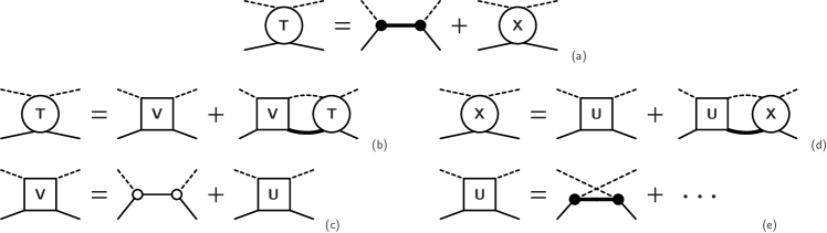
Figure 3: Generic structure of the pion-nucleon $T$ matrix employing pions and nucleons as the only hadronic degrees of freedom Haberzettl97 . (a) Splitting of $T$ into $s$-channel pole part and non-pole $X$. (b) Bethe-Salpeter integral equation for $T$, with (c) the driving term $V$ that contains an undressed $s$-channel exchange. (d) Bethe-Salpeter integral equation for non-pole $X$, with (e) fully dressed non-pole driving term $U$. Dressed vertices are represented by solid circles, while undressed ones are denoted by open circles. Dressed (internal) nucleons are shown as thick lines; undressed ones as thin lines; pions are shown as dashed lines. Note that the $s$-channel pole term in the driving term $V$ is bare [because it gets dressed by the equation (b) itself] whereas, in the full theory, all mechanisms in the non-pole $U$ are fully dressed via the Dyson-Schwinger-type mechanisms as shown in Fig. 4.

Even the simplest example, where the nucleon and pion propagators and their currents as well as the $\pi NN$ vertex are essentially bare, satisfies the generalized WTI of Eq. (9), as long as the masses are physical and the interaction current is the well-known Kroll-Ruderman current KR54 . The key to maintaining gauge invariance, therefore, is consistency among all ingredients of a particular formulation of the reaction dynamics. Exploiting this consistency requirement in cases where gauge invariance does not follow — which nearly always is the case as soon as one introduces any kind of dressing mechanisms — is found to be indeed a powerful tool for constraining the interaction current by ensuring the validity of Eq. (12) Haberzettl97 ; HBMF98a ; HNK06 ; HHN11 .

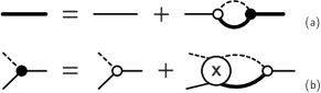
Figure 4: Dressing mechanisms for (a) the nucleon propagator $S$ and (b) the $\pi NN$ vertex $F$ according to Eq. (17) that appears in the nucleon’s self-energy contribution $\Sigma$ shown in (a) as a loop. The notation is the same as in Fig. 3.

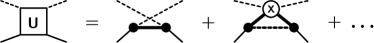
Figure 5: More detailed description of the driving term $U$ in Fig. 3(e). In addition to the basic $u$-channel exchange, $U$ also contains nonlinear contributions where the full amplitude $X$ given in Fig. 3(d) is dressed by hadron loops Haberzettl97 . (The lowest-order contribution from the nonlinear dressing mechanism of the second diagram on the right-hand side here appears in the fourth graph of Fig. 10.)

We will find, in Sec. IV, similar consistency constraints for the present problem of two-pion production. However, to understand better the structure of the problem, we need to look in more detail at some of the features of the dressing mechanisms resulting from the theoretical treatment of single-pion photoproduction of Ref. Haberzettl97 , since the underlying field theory for both single-pion and two-pion production is the same. The full dressing mechanisms of single-pion production originate from the Dyson-Schwinger-type structure that governs the pion-nucleon scattering problem whose equations are summarized diagrammatically in Figs. 3 and 4. There is no need here to recapitulate all features of the treatment of Ref. Haberzettl97 providing these structures. Relevant for the problem at hand is only the fact that the bare $\pi NN$ vertex $f$ from the underlying interaction Lagrangian is dressed by the non-polar part $X$ of the full $\pi N$ $T$ matrix, i.e.,

$$F=f+XG_{0}f$$ (17)

depicted in Fig. 4(b). Here, $X$ solves the Bethe-Salpeter-type equation,

$$X=U+UG_{0}X$$ (18)

shown in Fig. 3(d), whose non-polar driving term $U$ is given in the lowest order by the $u$-channel exchange of Fig. 3(e). At higher orders, $U$ also contains nonlinear contributions where the full $X$ itself is dressed by loops, as shown in the example of Fig. 5. (See also Ref. Haberzettl97 .) In principle, therefore, everything in Eq. (18) is dressed fully by the nonlinear Dyson-Schwinger mechanisms.

According to Eq. (5b), the four-point interaction current $M^{\mu}_{\text{int}}$ is obtained by applying the gauge derivative to the dressed vertex $F$. Using the explicit dressing equation (17), this reads Haberzettl97

$$M^{\mu}_{\text{int}}=\left(1+XG_{0}\right)f^{\mu}+X^{\mu}G_{0}f+XG_{0}d^{\mu}G_{0}f~{},$$ (19)

where $f^{\mu}$ is the (bare) Kroll-Ruderman current and $X^{\mu}$ is the five-point interaction current resulting from applying the gauge derivative to Eq. (18), i.e.,

$$X^{\mu}=\left(1+XG_{0}\right)U^{\mu}\left(G_{0}X+1\right)+XG_{0}d^{\mu}G_{0}X~{}.$$ (20)

Here, $U^{\mu}$ is the five-point interaction current (whose lowest order is shown in Fig. 6) obtained by coupling the photon to all elements of the driving term $U$. We see here that the internal dressing structure of the interaction current $M^{\mu}_{\text{int}}$ in Eq. (19) is quite complex; it contains, in particular, the full hadronic final-state interaction in terms of the non-polar $\pi N$ scattering matrix $X$. One can use Eq. (20) to bring Eq. (19) into a form better suited for practical applications, but there is no need to pursue this here (for more details; see Ref. Haberzettl97 for formal derivations and Refs. HNK06 ; HHN11 for practical aspects).

What we do need for the present purpose, however, is the proof that $X^{\mu}$ satisfies the usual gauge-invariant constraint of an interaction current. This proof was given already in Eq. (72) of Ref. Haberzettl97 , but we repeat it here because it will introduce the general techniques of handling such four-divergences that we will need later on. For this purpose, let us restrict $U$ to be given only by the $u$-channel exchange shown in Fig. 5. We emphasize that neglecting higher orders is done here only to simplify the derivation. In general, the proof will go through for any possible mechanism at any order Haberzettl97 . For a simple $u$-channel exchange, we may write $U$ as

$$U=F_{i}SF_{f}~{},$$ (21)

where the indices $i$ and $f$ on the dressed vertices $F$ indicate whether the corresponding pion leg is an initial or a final particle for the $\pi N\to\pi N$ process. The current $U^{\mu}\equiv-\{U\}^{\mu}$ resulting from coupling the photon to $U$ is then given by the three diagrams shown in Fig. 6, i.e.,

$$U^{\mu}=M^{\mu}_{i}SF_{f}+F_{i}SJ_{N}^{\mu}SF_{f}+F_{i}SM^{\mu}_{f}~{}.$$ (22)

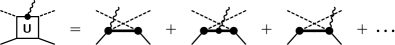
Figure 6: Contribution to the five-point interaction current $U^{\mu}$ based on coupling the photon to the interior of the lowest-order $u$-channel exchange in the non-polar driving term $U$ in Fig. 5. The currents arising from the higher-order loops are discussed in Ref. Haberzettl97 .

We note here that, because the photon couples into the fully dressed $\pi NN$ vertices of the $u$-channel exchange (21), the currents $M^{\mu}_{i}$ and $M^{\mu}_{f}$ are the full four-point interaction currents of Eq. (19), with $i$ and $f$ indicating the direction of the pion leg. This type of nonlinearity is a natural and unavoidable consequence of the fact that particle number is not conserved in any process involving mesons. Using the four-divergences of Eqs. (15) and (16), we obtain

$$k_{\mu}U^{\mu} =(\hat{Q}F_{i}-F_{i}\hat{Q})SF_{f}+F_{i}(\hat{Q}S-S\hat{Q})F_{f}$$

$$\quad\mbox{}+F_{i}S(\hat{Q}F_{f}-F_{f}\hat{Q})$$

$$=\hat{Q}U-U\hat{Q}~{},$$ (23)

Figure 7: Generic topological structure of the two-pion production current off another meson (depicted here as a heavy wavy line), with $\gamma\rho\to\pi\pi$ shown as an example. Attaching the photon to the hadronic $\pi\pi\rho$ vertex on the left produces a structure exactly analogous to the $\pi NN$ case, with three contributions arising from the external legs, and one from the interior interaction region.

and thus

$$k_{\mu}X^{\mu} =(1+XG_{0})(k_{\mu}U^{\mu})(G_{0}X+1)+XG_{0}(k_{\mu}d^{\mu})G_{0}X$$

$$=(1+XG_{0})(\hat{Q}U-U\hat{Q})(G_{0}X+1)$$

$$\qquad\mbox{}+X(\hat{Q}G_{0}-G_{0}\hat{Q})X$$

$$=\hat{Q}X-X\hat{Q}~{},$$ (24)

where

$$G_{0}(k_{\mu}d^{\mu})G_{0}=\hat{Q}G_{0}-G_{0}\hat{Q}$$ (25)

was used, which follows from the definition of $d^{\mu}$ and the WTIs of Eq. (16). Both four-divergences of $U^{\mu}$ and $X^{\mu}$, therefore, produce the generic structure associated with interaction currents discussed at the end of the preceding subsection. For this generic result to hold, it is irrelevant whether we are dealing with four-point currents like $M^{\mu}_{\text{int}}$ or five-point currents like $U^{\mu}$ or $X^{\mu}$. The result (24), in particular, will be relevant for the gauge-invariance proof of the two-pion photoproduction current given in Sec. IV in the context of Eq. (64).

II.3 Topologically analogous problem: $\gamma\rho\to\pi\pi$

The underlying field theory of single pion photoproduction just discussed above Haberzettl97 contains pions, nucleons, and photons as explicit degrees of freedom. The resulting topological structure is complete in the sense that even if in actual practical applications one needs to expand the meaning of “pion” and “nucleon” to generically stand for all possible mesons and baryons, respectively, this structure does not change. The situation is different for two-pion production processes because, as we will discuss in more detail in Sec. III, two pions can be produced not only sequentially off baryons but also directly through the decay of mesons, and this will add topological features to the problem that cannot be expressed in the generic picture of pions and nucleons alone with their interaction being described by the $\pi NN$ vertex. In the following, therefore, we need to introduce the $\rho$ meson as an additional generic meson degree of freedom that can decay into two pions, i.e.,

$$\rho\to\pi\pi~{}.$$ (26)

As with pions and nucleons, in an actual application, “rho” can then be expanded to subsume all mesons that can decay into two pions.

As far as the interaction with photons is concerned, we now also need to consider the photon-induced process,

$$\gamma\rho\to\pi\pi$$ (27)

as being on par with the $\gamma N\to\pi N$ reaction. Topologically, the production current for this reaction has the structure depicted in Fig. 7, which is in complete analogy to the pion production of the nucleon shown in Fig. 1 because both types of processes are based on the interaction of the photon with a hadronic three-point vertex.

Figure 8: Lowest-order non-polar $u$-channel exchanges for (a) $\pi\pi\to\pi\pi$ and (b) $\pi\rho\to\pi\rho$ scattering.

The hadronic final-state interaction of the $\pi\pi$ system for this process can be depicted in a structure similar to Fig. 3, with all external lines being pions and the primary interaction being given by the $\pi\pi\rho$ vertex. Relevant for the following, in particular, is the fact that one can also split the full $T$ matrix into a pole part and a non-pole part $X$ whose lowest-order driving term is a $u$-channel exchange as depicted in Fig. 8(a). The same is true for any meson-meson scattering problem whose basic interaction is described in terms of a bare three-meson vertex. Figure 8(b) shows the corresponding non-polar driving terms for $\pi\rho\to\pi\rho$.

As we shall see, the details of the underlying meson-meson scattering problem does not matter for the following. What matters is only the generic topological structure of the production current shown in Fig. 7 and the fact that non-polar contributions $X$ to the scattering amplitude satisfy a Bethe-Salpeter-type equation of the generic structure given in Eq. (18) that is driven at lowest order by non-polar $u$-channel exchanges, like the ones shown in Fig. 8. All other details can be left to be worked out in an actual application.

III Hadronic two-pion production

We now turn to the problem of the production of two pions off a nucleon. Before looking at the photon-induced process, we first consider all possible hadronic transitions

$$N\to\pi\pi N~{},$$ (28)

including all possible dressing mechanisms. We will then derive the associated photoproduction current by attaching the photon in all possible ways to the dressed hadronic process. This is done in complete analogy to how the single-pion-production current is obtained from the fully dressed $\pi NN$ vertex as visualized in Fig. 1.

Describing the process $N\to\pi\pi N$ within the generic field-theory framework of pions, rho mesons, and nucleons, there are three basic interaction vertices that are relatively easy to deal with, namely the three-hadron vertices $\pi NN$, $\pi\pi\rho$, and $\rho NN$. These interactions provide the basic sequential production mechanisms shown in Figs. 9(a) and 9(b). However, there exist also multi-pion processes where a meson decays into three or more pions that cannot be resolved experimentally as being due to a sequence of three-meson interactions. For the $\omega$ meson, for example, the dominant decay mode is $\omega\to\pi^{+}\pi^{0}\pi^{-}$. Hence, one of the simplest examples of two-meson production due to a four-meson interaction is depicted in Fig. 9(c) showing an intermediate $\omega\pi\pi\pi$ vertex where one of the pions is subsequently absorbed by the nucleon.

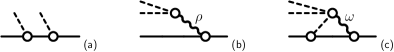
Figure 9: Basic two-pion production processes: (a) sequential production along the nucleon line, and (b) intermediate production of a $\rho$ meson decaying into two pions. Part (c) provides an example of another mechanism based on intermediate multi-pion vertices. In this example, an $\omega$ meson produced off the nucleon decays into three pions, with one pion subsequently being absorbed by the nucleon. The mesons $\rho$ and $\omega$ here subsume any meson having two-pion and three-pion decay modes, respectively.

It should be clear that the full dynamical treatment of processes initiated by the three-pion vertex requires at least a four-body treatment of the intermediate $\pi\pi\pi N$ system. In general, any process initiated by an $n$-pion meson vertex would require employing the dynamics of at least an $(n+1)$-body system. Such treatments clearly are beyond the scope of what is at present practically possible, and we will deal with this complication by, at first, ignoring multi-pion vertices like the one depicted in Fig. 9(c). We will restrict, therefore, the present formulation to the three-body dynamics of the $\pi\pi N$ system that is initiated by the two types of processes depicted in Figs. 9(a) and 9(b) based solely on three-hadron interactions. As we shall see, this does not exclude incorporating processes initiated by multi-pion vertices like the one in Fig. 9(c) at some later stage because all photo-processes that can be related to independent hadronic production mechanisms can be treated independently. Hence, we may safely ignore such multi-pion processes now, and we will revisit the problem later, in Appendix A.

For the time being, therefore, we only consider the two basic $N\to\pi\pi N$ processes initiated by the two bare transitions depicted in Figs. 9(a) and 9(b). Figure 10 shows the first few terms of higher-order loop corrections of the basic processes. In the figure, we have omitted all contributions that can be subsumed in the dressing mechanisms of individual three-point vertices. In other words, the diagrams shown in Fig. 10 depict the first few contributions of the multiple-scattering series describing the three-body final-state interaction (FSI) within the $\pi\pi N$ system.

Inspecting the diagrams in Fig. 10 and noting that the $u$-channel exchanges appearing there are the beginnings of the two-body multiple-scattering series,

$$X=U+UG_{0}U+\cdots~{},$$ (29)

it is a simple exercise to sum up all contributions up to the level of two dressed loops, i.e., the internal particle propagators and vertices in the resulting diagrams shown in Fig. 11 are fully dressed, and all meson-baryon and meson-meson FSI scattering processes are described by non-polar scattering matrices $X$ because all $s$-channel pole contributions are accounted for in fully dressed sequential two-meson vertices. In drawing Fig. 11, we have relaxed the restriction to nucleons, pions, and rho mesons, and allowed the graphs to subsume all possible meson and baryon states that may contribute to the process of $N\to\pi\pi N$. The diagrams are grouped into no-loop (NL), one-loop (1L) and two-loop (2L) contributions in increasing complexity of the hadronic final-state interactions mediated by non-polar $X$ amplitudes.

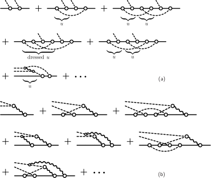
Figure 10: Hadronic two-pion production processes (a) along a nucleon line and (b) via an intermediate meson (wavy line) that can decay into two pions. Shown here for both cases are only those bare graphs up to the two-pion-loop level that do not contribute to the dressing of individual vertices, i.e., the loops shown here always straddle at least two vertices. The braces under the diagrams for (a) indicate basic $u$-channel-type exchanges. The $u$-channel exchange in the fourth diagram is dressed by a pion loop, corresponding to the nonlinear loop mechanism shown in the second diagram on the right-hand side of Fig. 5. The intermediate wavy line in the $u$-channel-type exchange of the last diagram in (a) indicates a meson that can couple to two pions. (Note that we could equally well interpret this as a $t$-channel exchange. In fact, when symmetrizing the indistinguishable physical pions, both types of exchanges are incorporated on an equal footing as a matter of course.)

We could now attach the photon to the hadronic diagrams in Fig. 11 and derive the corresponding production currents. The explicit results given in Sec. IV.2 presumably will be sufficient for most, if not all, practical purposes. For the fundamental theoretical understanding of the process, however, it would be interesting to derive a closed-form expression for the entire two-pion photo-process similar to what is possible for the single-pion production. And one would like to do so in a manner that maintains gauge invariance. To this end, we note that after the first interaction in the 1L graphs of Fig. 11, the $\pi\pi N$ system loses its memory about which of the two NL graphs of Fig. 11 was responsible for its initial creation and only retains the memory about the last two-body interaction, i.e., whether it was a $\pi N$ or a $\pi\pi$ reaction. Ignoring for the moment nonlinear effects that allow the creation of an arbitrary number of pions, all subsequent interactions, therefore, are governed by the dynamics of a three-body system. [We add here parenthetically that apart from the generic implications of a Dyson-Schwinger-type framework which is tantamount to having infinitely many mesons, the multi-pion aspect will also enter the picture through the driving-term’s nonlinearities discussed in the context of Eq. (35); see also Fig. 13.]

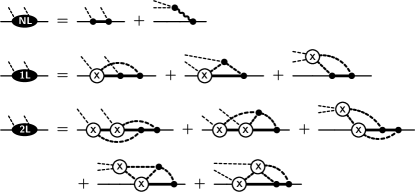
Figure 11: Grouping of hadronic two-pion production mechanisms off the nucleon involving no loop (NL), one loop (1L), and two loops (2L). (Anticipating the outcome of taking into account the symmetry of the indistinguishable pions, we do not differentiate between diagrams that differ only by labeling the two pions.) The thick interior lines subsume all particles permitted by the process with the solid lines indicating baryons and the dashed lines mesons. The thick wavy line stands for those mesons (like $\rho$, $\omega$, etc.) that can decay into two pions (for intermediate mesons, such mesons are subsumed under the heavy dashed line). Summations over all permitted internal particles are implied. All vertices are fully dressed and various meson-baryon or meson-meson scattering processes indicated by X are non-polar, i.e., they do not contain $s$-channel driving terms because their contributions are already subsumed in the full dressing of the vertices.

III.1 Alt-Grassberger-Sandhas equations

The solution of the non-relativistic quantum-mechanical three-body scattering problem was given by Faddeev Faddeev60 ; Faddeev . One of the most decisive aspects of the Faddeev approach is the manner in which the information about the sequence of interactions percolates through the system such that all interactions at all orders are possible, but double-counting of sequential interactions within the same two-body subsystem of the three particles is precluded, thus making the solutions unique. This basically is just an “accounting” problem and as such also valid in a relativistic context. We may therefore translate the structure of the Faddeev equations to the present problem by (1) simply assuming covariant relativistic kinematics, (2) realizing that the proper counterparts of the non-relativistic two-body $T$-matrices are the corresponding non-polar scattering matrices $X$ because non-relativistic potentials correspond to non-polar driving terms, and (3) allowing for non-trivial nonlinearities of the type analogous to those for the $\pi N$ problem depicted in Fig. 5.

The particular variant of the Faddeev approach we will use in the present work are the Alt-Grassberger-Sandhas (AGS) equations AGS67 ; Sandhas72 because they are given in terms of transition operators that are symmetric in their initial and final cluster configuration and thus can be applied to the present problem requiring only minor modifications related to relativistic kinematics and the fact that the particle number is not conserved.

First, to organize the information, we assume that the pions are distinguishable and label them as $\pi_{1}$ and $\pi_{2}$. (The indistinguishability of pions can easily be taken care of when calculating observables by appropriately symmetrizing the amplitudes.) Accordingly, we introduce three two-cluster channels $\alpha,\beta,\gamma=1,2,3$ by grouping the three particles as

“1” $$=(\pi_{1}N,\pi_{2})~{},$$

“2” $$=(\pi_{2}N,\pi_{1})~{},$$ (30)

“3” $$=(\pi_{1}\pi_{2},N)~{}.$$

Each ($2+1$) three-body configuration, therefore, consists of a two-body subsystem and a single-particle spectator. The indices $\alpha$, $\beta$, $\gamma$, etc. may also refer to the two-body subsystem of these two-cluster configurations.

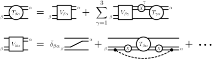
Figure 12: Generic structure of the Faddeev-type AGS three-body equations (31) and its driving terms (35). Depending on the cluster indices $\alpha$, $\beta$, and $\gamma$ defined in Eq. (30), two of the horizontal lines depict pions and one the nucleon. The (dashed) meson loop around $G_{0}X_{\beta}G_{0}T_{\beta\alpha}G_{0}X_{\alpha}G_{0}$ in the last diagram of the bottom line provides one (of many) nonlinear contributions to the solution (see also Fig. 13). The nature of the meson depends on which particles are connected by the loop.

The AGS equations AGS67 ; Sandhas72 can be written within the present context as

$$T_{\beta\alpha}=V_{\beta\alpha}+\sum_{\gamma=1}^{3}V_{\beta\gamma}G_{0}X_{\gamma}G_{0}T_{\gamma\alpha}~{},$$ (31)

with $\alpha,\beta,\gamma=1,2,3,$ where $T_{\beta\alpha}$ describes the transition from an initial two-cluster configuration $\alpha$ to the final configuration $\beta$. The equation is depicted in Fig. 12. For each two-body subsystem within the intermediate configurations $\gamma$, the full interaction is given by the corresponding non-polar scattering matrix $X$ of the two-body subsystem of $\gamma$ that has to be extended into the three-body space such that the propagation of the single spectator particle within $\gamma$ is unaffected. Hence, we may write in a generic manner,

$$X_{\gamma}=[X]_{\gamma}\circ t_{s,\gamma}^{-1}~{},$$ (32)

where $[\cdots]_{\gamma}$ denotes the restriction to the two-body subspace within the $\gamma$ cluster, and $t_{s,\gamma}$ is a generic notation for the single-particle spectator propagator within the $\gamma$ cluster. We thus have

$$G_{0}X_{\gamma}G_{0}=\left[G_{0}XG_{0}\right]_{\gamma}\circ t_{s,\gamma}~{},$$ (33)

where $G_{0}$ on the left-hand side describes the free intermediate propagation of the three particles within the $\pi\pi N$ system, i.e.,

$$G_{0}=\Delta_{1}(q_{\pi_{1}})\circ\Delta_{2}(q_{\pi_{2}})\circ S(p_{N})~{},$$ (34)

which is the straightforward three-body extension of the two-body $G_{0}$ of Eq. (2), whereas $G_{0}$ within the $[\cdots]_{\gamma}$ brackets denotes the two-body restriction as given in Eq. (2). The meaning of $G_{0}X_{\gamma}G_{0}$ within the present three-body context, therefore, is simply $[G_{0}XG_{0}]_{\gamma}$ as a two-body expression convoluted with the spectator propagator $t_{s,\gamma}$ of the free third particle that is unaffected by the two-body interaction $X$.

Figure 13: First two lowest-order contributions of the nonlinear dressing $N_{\beta\alpha}$ of the AGS driving term (35). The loop is seen here to straddle at least two $X$ amplitudes. Higher-order iterates of $T_{\beta\alpha}$ produce loops around any number of $X$ amplitudes.

The driving terms $V_{\beta\alpha}$ of Eq. (31) are given as

$$V_{\beta\alpha}=\bar{\delta}_{\beta\alpha}G^{-1}_{0}+N_{\beta\alpha}~{},$$ (35)

where

$$\bar{\delta}_{\beta\alpha}=1-\delta_{\beta\alpha}$$ (36)

is the anti-Kronecker symbol that vanishes if the initial and final two-body groupings of the $\pi\pi N$ system are the same. The elements $N_{\beta\alpha}$ describe the nonlinear dressing of $T_{\beta\alpha}$ in the manner depicted in Fig. 13, in analogy to the nonlinear $\pi N$ dressing mechanisms shown in Fig. 5. It is crucial here that this dressing happens around $G_{0}X_{\beta}G_{0}T_{\beta\alpha}G_{0}X_{\alpha}G_{0}$, i.e., the loop particle must connect particles of the initial and final two-body systems to avoid double-counting with the mechanisms described by Fig. 5 or with higher-order iterations of $X_{\gamma}$ contributions. Nonlinearities, like $N_{\beta\alpha}$, are absent from the original AGS equations AGS67 ; Sandhas72 because they assume the particle number to be conserved. For three-body processes involving pions, however, terms like this one are necessary in principle (even if it is very difficult to calculate in practice) because internally infinitely many pions may contribute.

We emphasize that there are limits to the three-body treatment of the $\pi\pi N$ system even if one takes into account nonlinear dressings of the driving terms of the kind shown in Fig. 12. For example, if the loop particle for the last graph in Fig. 12 is the nucleon, the AGS amplitude enclosed by the loop is a three-meson amplitude and thus outside the scope of the three-body treatment of the $\pi\pi N$ system. Moreover, in general, depending on how many mesons one considers to be created at intermediate stages, much more complicated $N$-body-type nonlinearities will result. It is possible in this way to recover some of the complexities of the problem associated with multi-pion vertices discussed in connection with the mechanism of Fig. 9(c), for example. We will consider additional three-body-force-type mechanisms associated with such processes in more detail in Appendix A. In general, of course, the actual calculation of such higher-order contributions in practical applications is quite challenging, to say the least, and we will, therefore, limit the detailed derivations in the following to the “pure” Faddeev contribution $\bar{\delta}_{\beta\alpha}G_{0}^{-1}$, and only mention in passing the ramifications of including nonlinearities in the driving term. Suffice it to say that the present formulation is consistent and correct for the system of two explicit pions and one nucleon where each of the particles may be fully dressed by any mechanism compatible with three-body dynamics.

Before we implement the AGS approach for the present problem, it is convenient to introduce a short-hand notation by defining operator-valued $3\times 3$ matrices according to

$${\textbf{{T}}}_{\beta\alpha} =T_{\beta\alpha}~{},$$ (37a)

$${\textbf{{V}}}_{\beta\alpha} =V_{\beta\alpha}~{},$$ (37b)

$$({\textbf{{G}}}_{{\textbf{{0}}}})_{\beta\alpha} =\delta_{\beta\alpha}G_{0}X_{\alpha}G_{0}~{}.$$ (37c)

This permits us to write the AGS equation (31) as a matrix equation in the form of

$${\textbf{{T}}}={\textbf{{V}}}+{\textbf{{V}}}{\textbf{{G}}}_{{\textbf{{0}}}}{\textbf{{T}}}~{},$$ (38)

which has the familiar Lippmann-Schwinger (LS) form of all scattering problems. Note in this context that the three-body dressing mechanism depicted in Fig. 13 corresponds to the dressing of ${\textbf{{G}}}_{{\textbf{{0}}}}{\textbf{{T}}}{\textbf{{G}}}_{{\textbf{{0}}}}$, i.e., exactly analogous to the dressing of $G_{0}XG_{0}$ depicted in the right-most diagram of Fig. 5 for the two-body $\pi N$ problem.

III.2 Three-body Faddeev treatment of hadronic two-pion production

Following the reasoning that the primary dynamics of the $\pi\pi N$ system beyond the one-loop level is given by three-body dynamics, the multiple-scattering series providing the final-state interactions within the $\pi\pi N$ system can be summed up in terms of the three-body transition operators $T_{\beta\alpha}$ of the AGS approach, and we immediately find that the hadronic two-pion production can be described by three components $M_{\beta}$ ($\beta=1,2,3$) given by

$$M_{\beta} =\sum_{\alpha}\left(\delta_{\beta\alpha}+\sum_{\gamma}T_{\beta\gamma}G_{0}X_{\gamma}G_{0}\bar{\delta}_{\gamma\alpha}\right)f_{\alpha}$$

$$\qquad\mbox{}+~{}\sum_{\gamma}\bigg{(}\delta_{\beta\gamma}+T_{\beta\gamma}G_{0}X_{\gamma}G_{0}\bigg{)}\sum_{\alpha}N_{\gamma\alpha}G_{0}f_{\alpha}~{},$$ (39)

where $f_{\alpha}$ describes the three basic production mechanisms shown in Fig. 14. The second term here is only present because of nonlinearities like those depicted in Fig. 13; it is absent in a standard three-body treatment. Expanding the right-hand side to second order in $X_{\gamma}$ produces

$$M_{\beta} =f_{\beta}+\sum_{\gamma,\alpha}\bar{\delta}_{\beta\gamma}\bar{\delta}_{\gamma\alpha}X_{\gamma}G_{0}f_{\alpha}$$

$$\qquad\mbox{}+\sum_{\gamma,\kappa,\alpha}\bar{\delta}_{\beta\gamma}\bar{\delta}_{\gamma\kappa}\bar{\delta}_{\kappa\alpha}X_{\gamma}G_{0}X_{\kappa}G_{0}f_{\alpha}$$

$$\qquad\mbox{}+\sum_{\alpha}N_{\beta\alpha}G_{0}f_{\alpha}\cdots$$ (40)

where the first three terms correspond precisely to the structure up to two loops shown in Fig. 11, with the terms here corresponding to the NL, 1L, and 2L graph groups of that figure. The lowest-order nonlinear effects contained in the last explicit term here are of second order in $X_{\gamma}$, like the preceding term, but they are of third order in the (dressed) loop structure, as shown in Fig. 15.

Figure 14: Definition of the basic $\pi\pi N$ vertices $f_{\alpha}$ assuming distinguishable pions. The pion lines of the first two diagrams are labeled accordingly. The cluster index $\alpha=1,2,3$ defined in Eq. (30) describes the hadron pair of the final three-point vertex in $f_{\alpha}$.

Figure 15: Lowest-order nonlinear contributions $N_{\beta\alpha}G_{0}f_{\alpha}$ employing the mechanism of Fig. 13. The internal meson lines (thick dashes) depicts any meson compatible with the process. The loops may connect any two particle respectively from the $\alpha$ and $\beta$ two-body systems, i.e., each graph here represents only one example of four possible contributions.

Defining formal three-component vectors with elements

$${\textbf{{f}}}_{\alpha} =f_{\alpha}~{},$$ (41a)

$${\textbf{{F}}}_{\beta} =\sum_{\alpha}\bar{\delta}_{\beta\alpha}f_{\alpha}~{},$$ (41b)

$$\tilde{{\textbf{{F}}}}_{\beta} =\sum_{\alpha}N_{\beta\alpha}G_{0}f_{\alpha}~{},$$ (41c)

$${\textbf{{M}}}_{\beta} =M_{\beta}~{},$$ (41d)

we may rewrite Eq. (39) as

$${\textbf{{M}}}=\left({\textbf{{I}}}+{\textbf{{T}}}{\textbf{{G}}}_{{\textbf{{0}}}}\right){\textbf{{F}}}+\left({\textbf{{1}}}+{\textbf{{T}}}{\textbf{{G}}}_{{\textbf{{0}}}}\right)\tilde{{\textbf{{F}}}}~{},$$ (42)

where the matrix I provides

$${\textbf{{I}}}{\textbf{{F}}}={\textbf{{f}}}\qquad\text{with}\qquad{\textbf{{I}}}_{\beta\alpha}=\tfrac{1}{2}-\delta_{\beta\alpha}~{}.$$ (43)

One easily verifies that I is indeed the inverse of the matrix whose elements are the anti-Kronecker symbols. Here, 1 is the unit matrix of the three-body system with elements $\delta_{\beta\alpha}$ and ${\textbf{{F}}}+\tilde{{\textbf{{F}}}}={\textbf{{V}}}G_{0}{\textbf{{f}}}$

In summary, the present description of the $N\to\pi\pi N$ process is given by

$$\mathbb{F}=\sum_{\beta}M_{\beta}=\sum_{\beta}{\textbf{{M}}}_{\beta}~{}.$$ (44)

The $\pi\pi NN$ “vertex” $\mathbb{F}$ constructed in this manner provides a complete description of the reaction dynamics at the three-body level of the dressed $\pi\pi N$ system (subject to the general limitations of three-body dynamics discussed earlier).

IV Attaching the Photon

Using the LSZ reduction, the full double-pion production current is given in terms of the gauge derivative by

$$M_{\pi\pi}^{\mu}=-G_{0}^{-1}\left\{G_{0}\mathbb{F}S\right\}^{\mu}S^{-1}~{},$$ (45)

where $S$ describes the incoming nucleon propagator and $G_{0}=\Delta_{1}\circ\Delta_{2}\circ S$ is the outgoing propagation of the free $\pi\pi N$ system. Hence, we have

$$M_{\pi\pi}^{\mu}=D^{\mu}G_{0}\mathbb{F}+\mathbb{F}^{\mu}+\mathbb{F}SJ_{N}^{\mu}~{},$$ (46)

where $J_{N}^{\mu}$ describes the current of the incoming nucleon. Here, $D^{\mu}$ is the three-body generalization of $d^{\mu}$ of Eq. (6), viz.

$$G_{0}D^{\mu}G_{0} \equiv-\left\{G_{0}\right\}^{\mu}$$

$$=(SJ^{\mu}_{N}S)\circ\Delta_{1}\circ\Delta_{2}+S\circ(\Delta_{1}J^{\mu}_{\pi_{1}}\Delta_{1})\circ\Delta_{2}$$

$$\quad\mbox{}+S\circ\Delta_{1}\circ(\Delta_{2}J^{\mu}_{\pi_{2}}\Delta_{2})~{},$$ (47)

i.e., it subsumes the three currents of the outgoing legs analogous to what is depicted in Fig. 2 for the two-body case. The five-point interaction current $\mathbb{F}^{\mu}\equiv-\{\mathbb{F}\}^{\mu}$ contains all mechanisms where the photon is attached to the interior of the hadronic two-pion production mechanisms given by Eq. (44).

Then with

$$k_{\mu}D^{\mu}=G_{0}^{-1}\hat{Q}-\hat{Q}G_{0}^{-1}$$ (48)

and the WTI of Eq. (10) for the nucleon current, the four-divergence of $M_{\pi\pi}^{\mu}$ reads

$$k_{\mu}M_{\pi\pi}^{\mu}=G_{0}^{-1}\hat{Q}G_{0}\mathbb{F}-\hat{Q}\mathbb{F}+k_{\mu}\mathbb{F}^{\mu}+\mathbb{F}\hat{Q}-\mathbb{F}S\hat{Q}S^{-1}~{},$$ (49)

which shows that the four-divergence of the interaction current $\mathbb{F}^{\mu}$, in analogy to Eq. (15), must be given by

$$k_{\mu}\mathbb{F}^{\mu}=\hat{Q}\mathbb{F}-\mathbb{F}\hat{Q}$$ (50)

to produce the generalized WTI,

$$k_{\mu}M_{\pi\pi}^{\mu}=G_{0}^{-1}\hat{Q}G_{0}\mathbb{F}-\mathbb{F}S\hat{Q}S^{-1}~{}.$$ (51)

This provides a conserved current in the usual manner when all external hadrons are on-shell. More explicit form of this result will be given later in Eq. (77).

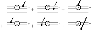
Figure 16: Representation of the current $({\textbf{{G}}}_{{\textbf{{0}}}}^{\mu})_{\beta\alpha}$ of Eq. (59). As in Fig. 12, two of the horizontal lines depict pions and one the nucleon. Note that the negative contribution of the spectator current in Eq. (60) cancels one of the spectator contributions of the two $D^{\mu}$ currents in Eq. (59), leaving only one spectator current given as the last diagram here.

IV.1 Proof of gauge invariance

To verify Eq. (50), let us define

$${\textbf{{M}}}^{\mu}\equiv-\left\{{\textbf{{M}}}\right\}^{\mu}$$ (52)

as the vector whose components provide $\mathbb{F}^{\mu}$ according to Eq. (44) as

$$\mathbb{F}^{\mu}=\sum_{\beta}{\textbf{{M}}}^{\mu}_{\beta}~{}.$$ (53)

Taking the gauge derivative of the matrix relation (42), the interaction-current component vector is given as

$${\textbf{{M}}}^{\mu} =\left({\textbf{{I}}}+{\textbf{{T}}}{\textbf{{G}}}_{{\textbf{{0}}}}\right)\tilde{{\textbf{{F}}}}^{\mu}+{\textbf{{T}}}^{\mu}{\textbf{{G}}}_{{\textbf{{0}}}}\tilde{{\textbf{{F}}}}+{\textbf{{T}}}{\textbf{{G}}}_{{\textbf{{0}}}}^{\mu}\tilde{{\textbf{{F}}}}~{},$$ (54)

where

$${\textbf{{T}}}^{\mu}=\left({\textbf{{1}}}+{\textbf{{T}}}{\textbf{{G}}}_{{\textbf{{0}}}}\right){\textbf{{V}}}^{\mu}\left({\textbf{{G}}}_{{\textbf{{0}}}}{\textbf{{T}}}+{\textbf{{1}}}\right)+{\textbf{{T}}}{\textbf{{G}}}_{{\textbf{{0}}}}^{\mu}{\textbf{{T}}}$$ (55)

is a straightforward consequence of applying the gauge derivative to the LS equation (38), in complete analogy to $X^{\mu}$ of Eq. (20). Hence,

$${\textbf{{M}}}^{\mu}=\left({\textbf{{I}}}+{\textbf{{T}}}{\textbf{{G}}}_{{\textbf{{0}}}}\right)\tilde{{\textbf{{F}}}}^{\mu}+\left({\textbf{{1}}}+{\textbf{{T}}}{\textbf{{G}}}_{{\textbf{{0}}}}\right){\textbf{{K}}}^{\mu}\left({\textbf{{1}}}+{\textbf{{T}}}{\textbf{{G}}}_{{\textbf{{0}}}}\right)\tilde{{\textbf{{F}}}}~{},$$ (56)

where the elements of $\tilde{{\textbf{{F}}}}^{\mu}$,

$$\tilde{{\textbf{{F}}}}^{\mu}_{\beta}=\sum_{\alpha}\bar{\delta}_{\beta\alpha}{\textbf{{F}}}^{\mu}_{\alpha}~{},\quad\text{with}\quad{\textbf{{F}}}^{\mu}_{\alpha}=-\left\{{\textbf{{F}}}_{\alpha}\right\}^{\mu}~{},$$ (57)

are the interaction currents associated with the elementary processes depicted in Fig. 14, and

$${\textbf{{K}}}^{\mu}\equiv-\left\{{\textbf{{V}}}{\textbf{{G}}}_{{\textbf{{0}}}}\right\}^{\mu}={\textbf{{V}}}^{\mu}{\textbf{{G}}}_{{\textbf{{0}}}}+{\textbf{{V}}}{\textbf{{G}}}_{{\textbf{{0}}}}^{\mu}$$ (58)

is the current associated with the kernel of the LS equation (38). The current matrix ${\textbf{{G}}}_{{\textbf{{0}}}}^{\mu}$ reads

$$({\textbf{{G}}}_{{\textbf{{0}}}}^{\mu})_{\beta\alpha}=\delta_{\beta\alpha}G_{0}\big{(}D^{\mu}G_{0}X_{\alpha}+X^{\mu}_{\alpha}+X_{\alpha}G_{0}D^{\mu}\big{)}G_{0}~{},$$ (59)

where, using Eq. (32), we obtain

$$X^{\mu}_{\alpha} \equiv-\left\{X_{\alpha}\right\}^{\mu}$$

$$=[X^{\mu}]_{\alpha}\circ t_{s,\alpha}^{-1}-[X]_{\alpha}\circ J^{\mu}_{s,\alpha}~{},$$ (60)

which is the three-body extension of the two-body interaction current $[X^{\mu}]_{\alpha}$. The current of the spectator particle within the three-body cluster $\alpha$ is represented by $J^{\mu}_{s,\alpha}\equiv\{t_{s,\alpha}^{-1}\}^{\mu}$. The negative sign of this term is crucial for avoiding double-counting of spectator contributions. In Eq. (59), for example, it cancels out one of the spectator $D^{\mu}$ currents in (59), as shown in Fig. 16.

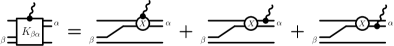
Figure 17: Interaction-current matrix element ${\textbf{{K}}}^{\mu}_{\beta\alpha}$ of the kernel of the AGS equation with explicit terms shown in the approximation of Eq. (63), i.e., without nonlinear terms $N_{\beta\alpha}$. As in Fig. 12, two of the horizontal lines depict pions and one the nucleon. In this approximation, due to the cancelation mechanism explained in the caption of Fig. 16, there is no current associated with the spectator particle, i.e., only the first three diagrams of Fig. 16 contribute.

In detail, the AGS-kernel matrix is given by

$$({\textbf{{V}}}{\textbf{{G}}}_{{\textbf{{0}}}})_{\beta\alpha}=\bar{\delta}_{\beta\alpha}X_{\alpha}G_{0}+N_{\beta\alpha}G_{0}X_{\alpha}G_{0}~{}.$$ (61)

If we neglect the nonlinearities $N_{\beta\alpha}$, we have

$${\textbf{{K}}}^{\mu}_{\beta\alpha}\to{\textbf{{K}}}^{\mu}_{\beta\alpha}={\textbf{{V}}}_{\beta\alpha}G_{0}\big{(}X_{\alpha}^{\mu}G_{0}+X_{\alpha}G_{0}D^{\mu}G_{0}\big{)}~{}.$$ (62)

Using Eqs. (47) and (60), we may write this as

$${\textbf{{K}}}^{\mu}_{\beta\alpha}\to{\textbf{{K}}}^{\mu}_{\beta\alpha}={\textbf{{V}}}_{\beta\alpha}G_{0}\big{[}X^{\mu}G_{0}+XG_{0}d^{\mu}G_{0}\big{]}_{\alpha}~{},$$ (63)

as shown in Fig. 17. In this approximation, therefore, using the known four-divergences of $X^{\mu}$ and $d^{\mu}$ given in Eqs. (24) and (25), one immediately obtains

$$k_{\mu}{\textbf{{K}}}^{\mu}=\hat{Q}{\textbf{{V}}}{\textbf{{G}}}_{{\textbf{{0}}}}-{\textbf{{V}}}{\textbf{{G}}}_{{\textbf{{0}}}}\hat{Q}~{}.$$ (64)

One may use here $\hat{Q}$ for the entire three-body system, even though Eqs. (24) and (25) only contain the corresponding operator for the two-body subsystem, because the spectator contribution of $\hat{Q}$, along the lower line on the right-hand side of Fig. 17, cancels between the two terms on the right-hand side of Eq. (64) since no interaction takes place along that line. One can show that the result (64) remains true even if the nonlinearities $N_{\beta\alpha}$ are taken into account. The proof requires tedious calculations and is not very illuminating; it will be omitted here.

To evaluate the four-divergence of ${\textbf{{M}}}^{\mu}$, we use the four-divergence (64) and the fact that the current $\tilde{{\textbf{{F}}}}^{\mu}$ satisfies the generic relations of any interaction-type current, i.e.,

$$k_{\mu}\tilde{{\textbf{{F}}}}^{\mu}=\hat{Q}\tilde{{\textbf{{F}}}}-\tilde{{\textbf{{F}}}}\hat{Q},$$ (65)

and then we easily find

$$k_{\mu}{\textbf{{M}}}^{\mu}=\hat{Q}{\textbf{{M}}}-{\textbf{{M}}}\hat{Q}~{},$$ (66)

which upon using Eq. (53) immediately verifies the validity of Eq. (50) as stipulated. Hence, the current $M_{\pi\pi}^{\mu}$ of Eq. (46) constructed with the help of the hadronic mechanisms (42) is indeed (locally) gauge invariant, and its generalized WTI is given by Eq. (51).

We can now write down the closed-form equation,

$$M_{\pi\pi}^{\mu}=\sum_{\beta}\left(D^{\mu}G_{0}M_{\beta}+M_{\beta}^{\mu}+M_{\beta}SJ_{N}^{\mu}\right)$$ (67)

for the full two-pion photoproduction current $M_{\pi\pi}^{\mu}$, where

$$M^{\mu}_{\beta}\equiv{\textbf{{M}}}^{\mu}_{\beta}$$ (68)

is the two-body component of ${\textbf{{M}}}^{\mu}$ in Eq. (56) that contains the full three-body final-state interactions of the problem. For practical applications, this presumes that the full two-pion production mechanisms $M_{\beta}$ of Eq. (39) can be calculated. In view of their complexity, this cannot be done easily in practice. One can show, however, that one can expand the full current in contributions of increasing complexity, similar to the NL, 1L, and 2L contributions in Fig. 11, which satisfy independent WTIs of their own. Maintaining local gauge invariance, therefore, is not predicated on being able to calculate the full current $M_{\pi\pi}^{\mu}$.

IV.2 Expanding the two-pion production current

To see how one may expand the full current, we define

$${\textbf{{M}}}_{0}={\textbf{{F}}}\quad\text{and}\quad{\textbf{{M}}}_{i}=\left({\textbf{{V}}}{\textbf{{G}}}_{{\textbf{{0}}}}\right)^{i}\tilde{{\textbf{{F}}}}\quad\text{for}\quad i=1,2,3,\ldots~{},$$ (69)

which implies, formally, that M of Eq. (42) can be written as

$${\textbf{{M}}}=\sum_{i=0}^{\infty}{\textbf{{M}}}_{i}~{}.$$ (70)

Note that, without the nonlinearities $N_{\beta\alpha}$, the matrix elements of the AGS kernel ${\textbf{{V}}}{\textbf{{G}}}_{{\textbf{{0}}}}$ are just given by $\bar{\delta}_{\beta\alpha}X_{\alpha}G_{0}$, as seen from Eq. (61). The expansion (70), therefore, provides the three-body multiple-scattering series of the final-state interactions within the $\pi\pi N$ system as a sequence of two-body interactions $X_{\alpha}$. One can show very easily, by the same techniques used in verifying the gauge invariance of the full current $M_{\pi\pi}^{\mu}$ that the same is true order by order by coupling the photon to ${\textbf{{M}}}_{i}$.

For the NL graphs of ${\textbf{{M}}}_{0}$, whose components are shown in Fig. 14, the two-pion currents depicted in Fig. 18 are gauge invariant as a matter of course because the corresponding gauge-invariant subprocess currents indicated by $M$ in the diagrams trivially add up to make each of the NL₁ and NL₂ currents in Fig. 18 gauge invariant separately. This can be found immediately by taking the four-divergence of each current. These are simple examples for something which is generally true: Coupling the photon to topologically independent hadronic processes (like the two distinct processes summed up in the NL contributions of Fig. 11) will produce naturally independent gauge-invariance constraints. This means that each component of ${\textbf{{M}}}_{0}={\textbf{{F}}}$ is gauge invariant separately. Since the components of $\tilde{{\textbf{{F}}}}^{\mu}$ are given by sums of NL currents, this also implies an explicit proof for the gauge-invariance relation (65).

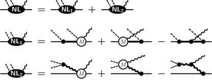
Figure 18: Two-pion photoproduction at the no-loop level where the photon is attached to the NL diagrams of Fig. 11. The two contributions NL₁ and NL₂ correspond to the two NL diagrams in Fig. 11 in the given order. The photoproduction amplitudes labeled $M$ are comprised of four generic terms each, similar to the pion-production case shown in Fig. 1 or the $\pi\pi$-production of Fig. 7. The subtractions correct the double counting resulting from the photon being attached to the respective intermediate particle in both preceding diagrams, i.e., when expanding all amplitudes $M$, each group consists of seven topologically distinc diagrams (see also Fig. 22). Each group of NL₁ and NL₂ diagrams satisfies an independent gauge-invariance constraint.

To investigate the gauge invariance of higher-order currents, we only need to look at the properties of the interaction-type currents ${\textbf{{M}}}^{\mu}_{i}\equiv-\left\{{\textbf{{M}}}_{i}\right\}^{\mu}$ because the contributions resulting from the four external legs of any $\gamma N\to\pi\pi N$ current are trivial. We must show, therefore, that each of such currents satisfies a constraint similar to Eq. (50). We write

$${\textbf{{W}}}\equiv({\textbf{{V}}}{\textbf{{G}}}_{{\textbf{{0}}}})^{i}$$ (71)

and find for the current ${\textbf{{W}}}^{\mu}\equiv-\left\{({\textbf{{V}}}{\textbf{{G}}}_{{\textbf{{0}}}})^{i}\right\}^{\mu}$,

$${\textbf{{W}}}^{\mu} =\sum_{k=0}^{i-1}\left({\textbf{{V}}}{\textbf{{G}}}_{{\textbf{{0}}}}\right)^{k}{\textbf{{K}}}^{\mu}\left({\textbf{{V}}}{\textbf{{G}}}_{{\textbf{{0}}}}\right)^{i-1-k}~{},$$ (72)

which gives its four-divergence as

$$k_{\mu}{\textbf{{W}}}^{\mu} =\sum_{k=0}^{i-1}\left({\textbf{{V}}}{\textbf{{G}}}_{{\textbf{{0}}}}\right)^{k}(\hat{Q}{\textbf{{V}}}{\textbf{{G}}}_{{\textbf{{0}}}}-{\textbf{{V}}}{\textbf{{G}}}_{{\textbf{{0}}}}\hat{Q})\left({\textbf{{V}}}{\textbf{{G}}}_{{\textbf{{0}}}}\right)^{i-1-k}$$

$$=\hat{Q}{\textbf{{W}}}-{\textbf{{W}}}\hat{Q}~{}.$$ (73)

This indeed is the generic result for an interaction-type current. With

$${\textbf{{M}}}^{\mu}_{i}={\textbf{{W}}}^{\mu}\tilde{{\textbf{{F}}}}+{\textbf{{W}}}\tilde{{\textbf{{F}}}}^{\mu}~{},$$ (74)

we thus find

$$k_{\mu}{\textbf{{M}}}^{\mu}_{i} =(\hat{Q}{\textbf{{W}}}-{\textbf{{W}}}\hat{Q})\tilde{{\textbf{{F}}}}+{\textbf{{W}}}(\hat{Q}\tilde{{\textbf{{F}}}}-\tilde{{\textbf{{F}}}}\hat{Q})$$

$$=\hat{Q}{\textbf{{M}}}_{i}-{\textbf{{M}}}_{i}\hat{Q},$$ (75)

which, once again, provides the generic gauge-invariance constraint for interaction currents. In other words, in view of the trivial gauge-invariance contributions from external legs, the current

$${\textbf{{M}}}_{i,\pi\pi}^{\mu}=D^{\mu}G_{0}{\textbf{{M}}}_{i}+{\textbf{{M}}}^{\mu}_{i}+{\textbf{{M}}}_{i}SJ_{N}^{\mu}$$ (76)

is also gauge invariant for each two-body component $\beta$ of this equation.

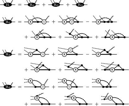
Figure 19: Two-pion-production currents resulting from coupling the photon to the 1L diagrams in Fig. 11. The subtractions correct double counting of the corresponding mechanisms. Expanding each four-point current labeled $M$ into its generic four terms, all current groups comprise ten diagrams each. Attaching the photon to the interior of $X$, as indicated in the respective fourth diagram of each group, produces the five-point interaction current $X^{\mu}$ detailed in Eq. (20) (see also Fig. 6 in Ref. Haberzettl97 ). Each group 1L_i ($i=1,2,3$) obeys an independent gauge-invariance constraint.

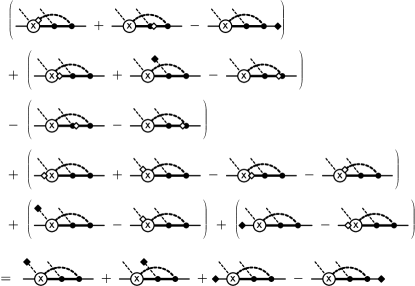
Figure 20: Graphical proof of gauge invariance for the 1L₁ current of Fig. 19. Each bracketed group above the equal sign corresponds to the four-divergence of one of the six graphs of 1L₁ in the same order as they appear in Fig. 19. In other words, the contents of each group is the result of applying the appropriate WTI to the corresponding current. The open diamond symbols indicate the action of the $\hat{Q}$ charge operators and show where the photon four-momentum $k$ needs to be injected into the hadronic graphs so that the four external hadron momenta are exactly the same as for the photo-process. If the diamond sits right next to a vertex or the amplitude $X$, there is no propagator between the diamond and the vertex or amplitude along that leg because it was canceled by the inverse propagators in the corresponding Ward-Takahashi identities (16); see text. The solid diamond symbols at the ends of some external legs indicates that in addition to a momentum $k$ being injected, there are residual inverse propagators with the four-momenta of the respective external particles that vanish when taken on-shell. Hence, the resulting expression in the last line, given explicitly in Eq. (77), vanishes if all four external hadrons are on-shell, thus providing a conserved current.

This consideration shows that attaching the photon in all possible ways to any topologically independent hadronic production process will provide an independent current that is constrained by its own Ward-Takahashi-type identity. The two topologically independent NL processes depicted in Fig. 18 are among the simplest examples for this fact. Figure 19 provides the currents resulting from attaching the photon to the three 1L diagrams of Fig. 11. The three independent currents labeled 1L_i ($i=1,2,3$) in Fig. 19 must be gauge invariant separately. The corresponding proofs are implied by the result found in Eq. (75). Nevertheless, we shall prove gauge invariance for the example of the current 1L₁ in Fig. 19 because it comprises contributions from single-particle currents, single-meson production currents, and the five-point interaction currents $X^{\mu}$ given in Eq. (20), and thus provides a non-trivial explicit example of how the consistency among all contributing current mechanisms ensures gauge invariance of the entire process. The procedure is most transparent in the graphical manner as shown in Fig. 20. Writing the underlying hadronic process, i.e., the first of the three 1L diagrams in Fig. 11, as $H_{\pi\pi}$ and the corresponding current as $H_{\pi\pi}^{\mu}$, its four-divergence can now simply be read from the final line in Fig. 20 as

$$k_{\mu}H_{\pi\pi}^{\mu} =\Delta_{1}^{-1}(q_{1})Q_{\pi_{1}}\Delta_{1}(q_{1}-k)\,H_{\pi\pi}^{(\pi_{1})}$$

$$\quad\mbox{}+\Delta_{2}^{-1}(q_{2})Q_{\pi_{2}}\Delta_{2}(q_{2}-k)\,H_{\pi\pi}^{(\pi_{2})}$$

$$\quad\mbox{}+S^{-1}(p^{\prime})Q_{N_{f}}S(p^{\prime}-k)\,H_{\pi\pi}^{(N_{f})}$$

$$\quad\mbox{}-H_{\pi\pi}^{(N_{i})}\,S(p+k)Q_{N_{i}}S^{-1}(p)~{},$$ (77)

where the explicit four-momenta are those of the photo-process

$$\gamma(k)+N_{i}(p)\to\pi_{1}(q_{1})+\pi_{2}(q_{2})+N_{f}(p^{\prime})$$ (78)

in a self-explanatory symbolic notation. The functions $H^{(h)}_{\pi\pi}$ describe the hadronic process $H_{\pi\pi}$ in the respective dynamical situations of the four diagrams of the final line in Fig. 20, i.e., $h=\pi_{1}$, $\pi_{2}$, $N_{f}$ indicate that, as compared to the momentum dependence of the photo-process, the corresponding outgoing pion or nucleon leg is reduced by the photon momentum $k$, and for $h=N_{i}$, the initial nucleon leg is increased by $k$. The momenta at the four external hadron legs of each $H^{(h)}_{\pi\pi}$, therefore, add up to conserve the overall four-momentum, similar to the photo-process (78). Equation (77) is completely analogous to the generalized WTI for the single-pion photoproduction given in Eq. (9).

The off-shell result (77) is the appropriate generalized WTI for any two-pion production current resulting from a topologically distinct hadronic two-pion production process $H_{\pi\pi}$. It is true for any one of the hadronic processes depicted in Fig. 11, and it will remain true for any one of the higher-order loop contributions.

Similar to the one-loop currents of Fig. 19, one can now easily derive as well the currents for the two-loop graphs in Fig. 11. Each group of 13 current diagrams resulting from each of the two-loop hadron graphs in Fig. 11 is then gauge invariant separately. Moreover, higher-order-loop contributions can be constructed by expanding the hadron equation (39) beyond what is given in Eq. (40). In general, each gauge-invariant group of graphs with $n$ loops consists of $7+3n$ members of which $5+n$ graphs contain a three-point current along a hadron line and $2+2n$ contain a four-point current resulting from the photon interaction with the interior of a three-hadron vertex. Each of these $n$-loop extensions is straightforward and may be easily derived following the examples given here explicitly. However, we expect that for most, if not all, practical purposes, the NL and 1L currents of Figs. 18 and 19 may be sufficient, and so we see no immediate need to go into more details here.

Before closing this section, we reiterate that in the formalism presented here, nucleons, pions and rho mesons are to be understood as generic placeholders for any and all baryonic or mesonic states compatible with the reaction in question. In particular, all intermediate states must subsume all baryons and mesons allowed for a particular reaction. This means that the nucleon lines in the intermediate states in the diagrams in Figs. 18 and 19 represent not only the nucleons but also any baryons that may contribute to the process at hand, i.e., the baryon resonances. Also, the pion as well as the $\rho$ meson lines appearing in the intermediate states in those diagrams represent any meson that may contribute. In two-pion photoproduction, for example, one of the relevant baryons in the intermediate states is the $\Delta$ which couples strongly to $\pi N$. For the same process, the $\sigma$ meson should also be taken into account wherever the $\rho$ meson appears since both mesons couple strongly to $\pi\pi$. Moreover, pure transverse transition-current contributions such as due to the Wess-Zumino anomalous couplings $\gamma\pi\rho$ and $\gamma\pi\omega$, which have no bearing on gauge invariance, should also be included.

V Possible Approximation Scheme

The evaluation of the full two-pion photoproduction amplitude as derived in Sec. IV is practically not feasible due to, in particular, its nonlinear character. This calls for an approximation scheme to make the problem tractable in practice. While there may be many ways to approximate the full amplitude given by Eq. (67), we would like to advocate that — as alluded to already — a scheme that preserves the increasing complexity of the reaction dynamics in terms of dressed loop structures as presented in the no-loop and one-loop examples of Figs. 18 and 19, respectively, is best suited to reflect the underlying physics. This loop expansion corresponds to an expansion in powers of the two-body hadronic interaction $X_{\gamma}$. We know, of course, that even at the levels of individual loops this is largely an intractable problem if the loop ingredients are to be calculated completely because of, again, the nonlinear dynamics of the required four-point interaction currents for single-meson production Haberzettl97 that enter the internal reaction mechanisms of such loops. However, efficient approximation schemes have been developed to deal with this complication at the four-point-function level (see, for example, Refs. Haberzettl97 ; HBMF98a ; HNK06 ; HHN11 ; HDHH12 , and references therein). Because of its off-shell nature, the requirement of local gauge invariance, in particular, proved to be an invaluable tool for helping link contributing dynamical mechanisms in a consistent manner (as described in the Introduction for the example of $NN$ bremsstrahlung NH09 ; HN10 ). We can make use of the experience gained there to treat the present five-point function dynamics of two-meson production in a similar manner, by demanding that all approximate steps fully preserve local gauge invariance as an off-shell constraint.

The (dressed) loop structure described in the previous section can be enumerated in terms of a multiple-scattering series in powers of $X_{\gamma}$ according to Eqs. (39) and (40) for the underlying hadronic $N\to\pi\pi N$ vertex $\mathbb{F}$ of Eq. (44). Formally, we may write

$$\mathbb{F}=\sum_{i=0}^{\infty}\mathbb{F}_{i}\ ,$$ (79)

where the index $i$ enumerates the relevant powers of $X_{\gamma}$, resulting in

$$\mathbb{F}_{0} \equiv\sum_{\beta}f_{\beta}\ ,$$ (80a)

$$\mathbb{F}_{1} \equiv\sum_{\beta}\Big{(}\sum_{\gamma,\alpha}\bar{\delta}_{\beta\gamma}\bar{\delta}_{\gamma\alpha}X_{\gamma}G_{0}f_{\alpha}\Big{)}\ ,$$ (80b)

$$\mathbb{F}_{2} \equiv\sum_{\beta}\Big{(}\sum_{\gamma,\kappa,\alpha}\bar{\delta}_{\beta\gamma}\bar{\delta}_{\gamma\kappa}\bar{\delta}_{\kappa\alpha}X_{\gamma}G_{0}X_{\kappa}G_{0}f_{\alpha}$$

$$\quad\mbox{}\quad\mbox{}\quad\mbox{}+\sum_{\alpha}N_{\beta\alpha}G_{0}f_{\alpha}\Big{)}~{},$$ (80c)

etc. The explicit expressions here correspond to the NL, 1L, and 2L contributions depicted in Fig. 11, of course.

V.1 Phenomenological hadronic contact vertex

In practice, we suggest to truncate the infinite sum (79) at some order $n$,

$$\mathbb{F}\approx\sum_{i=0}^{n}\mathbb{F}_{i}+\mathbb{C}~{},$$ (81)

and account for all higher orders by a remainder term $\mathbb{C}$ that is to be constructed phenomenologically as a contact term (free of singularities) by making an ansatz modeled after the Dirac and isospin structures of the full vertex $\mathbb{F}$.

To this end, we note that the most general (Dirac) structure of the full reaction amplitude $\mathbb{F}$ for

$$N(p)\to\pi(q_{1})+\pi(q_{2})+N(p^{\prime})~{},$$ (82)

where the arguments indicate the corresponding four-momenta, may be written as

$$\mathbb{F} =a_{1}+a_{2}\frac{\not{p}}{m}+a_{3}\frac{\not{p}^{\prime}}{m^{\prime}}+a_{4}\frac{\not{p}^{\prime}\not{p}}{m^{\prime}m}$$

$$+b_{1}\frac{\not{q}}{m_{\pi}}+b_{2}\frac{\not{q}\not{p}}{m_{\pi}m}+b_{3}\frac{\not{p}^{\prime}\not{q}}{m^{\prime}m_{\pi}}+b_{4}\frac{\not{p}^{\prime}\not{q}\not{p}}{m^{\prime}m_{\pi}m}\ ,$$ (83)

where $q\equiv q_{1}-q_{2}$ and the coefficients $a_{i}$ and $b_{i}$ $(i=1,2,3,4)$ are, in general, complex scalar functions of the momenta. Here, $m$, $m^{\prime}$, and $m_{\pi}$, respectively, stand for the masses of the initial nucleon, final nucleon, and produced pion.

The most general structure of $\mathbb{F}$ in isospin space is

$$\mathbb{F}=A\left(\hat{\pi}_{1}\cdot\hat{\pi}_{2}\right)+B\left(\hat{\pi}_{1}\times\hat{\pi}_{2}\right)\cdot\vec{\tau}\ ,$$ (84)

where $\hat{\pi}_{i}\ (i=1,2)$ denotes the outgoing pion fields in isospin space and $\vec{\tau}$ is the usual Pauli (isospin) operator. The Dirac structures of coefficients $A$ and $B$ here take the form given by Eq. (83).

Both the Dirac and isospin structures of the full amplitude $\mathbb{F}$ given by Eqs. (83) and (84) hold also for any term $\mathbb{F}_{i}$ in Eq. (79), i.e., at any order in powers of $X_{\gamma}$. This means, in particular, that the Dirac structure of $\mathbb{F}$ also carries over to the remainder term $\mathbb{C}$ independent of the truncation order $n$. A natural phenomenological ansatz for $\mathbb{C}$, therefore, would be to use the Dirac structure (83) and replace all eight coefficients $a_{i}$, $b_{i}$ ($i=1,2,3,4$) by individual phenomenological form factors with parameters that can be fitted to experimental data. The resulting expressions are presented in Appendix B for future reference.

In the application given below, in Sec. VI, we have pursued the simpler approximation of introducing one overall common form factor. This approximate ansatz is described in the following. Ignoring the isospin structure for now, we put

$$\mathbb{C} =\bigg{(}a_{1}+a_{2}\frac{\not{p}}{m}+a_{3}\frac{\not{p}^{\prime}}{m^{\prime}}+a_{4}\frac{\not{p}^{\prime}\not{p}}{m^{\prime}m}+b_{1}\frac{\not{q}}{m_{\pi}}$$

$$\qquad\mbox{}+b_{2}\frac{\not{q}\not{p}}{m_{\pi}m}+b_{3}\frac{\not{p}^{\prime}\not{q}}{m^{\prime}m_{\pi}}+b_{4}\frac{\not{p}^{\prime}\not{q}\not{p}}{m^{\prime}m_{\pi}m}\bigg{)}F~{},$$ (85)

where the coefficients $a_{i}$, $b_{i}$ ($i=1,2,3,4$) are now simple (complex) fit constants (that may also parametrically depend on the Mandelstam variable $s$ because it is a constant for a given experiment). As described in Appendix B.1, the form factor

$$F=F(p^{\prime 2},q_{1}^{2},q_{2}^{2};p^{2})$$ (86)

is a scalar function of the squared external four-momenta. We may take $F$ to be normalized to unity when all particles are on their respective mass shells, i.e.,

$$F(m^{\prime 2},m_{1}^{2},m_{2}^{2};m^{2})=1~{},$$ (87)

where $m_{1}$ and $m_{2}$ are the physical masses of the two pions. The detailed functional form of $F$ is irrelevant for now, but, in general, $F$ may contain further fit parameters (see also Sec. VI).

At this point a remark is in order. Although the analyticity and covariance of the full reaction amplitude $\mathbb{F}$ is preserved in the contact approximation for the higher-order loop contribution described above, unitarity is violated. To maintain unitarity in any type of approximation requires the complex phase structure of the reaction amplitude to be adjusted consistently as well. This is a highly non-trivial issue and beyond the scope of the present work.

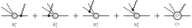
Figure 21: Phenomenological current $\mathbb{R}^{\mu}$ given by Eq. (89) subsuming higher-order loop contributions. The hadronic four-point vertex labeled $\mathbb{C}$ is the contact term introduced by Eq. (81), with its phenomenological form given by (85), and the last diagram depicts the five-point contact current $\mathbb{C}^{\mu}$, whose on-shell form is given in Eq. (91).

V.2 Phenomenological current for higher-order loops

The next step is to construct a two-pion production current $\mathbb{R}^{\mu}$ that results from the mechanisms subsumed in $\mathbb{C}$. Using the loop expansion, the full photoproduction amplitude of Eq. (45) may be written as

$$M^{\mu}_{\pi\pi} =\sum_{i=0}^{\infty}\left(-G_{0}^{-1}\{G_{0}\mathbb{F}_{i}S\}^{\mu}S^{-1}\right)$$

$$\approx\sum_{i=0}^{n}\left(-G_{0}^{-1}\{G_{0}\mathbb{F}_{i}S\}^{\mu}S^{-1}\right)+\mathbb{R}^{\mu}$$

$$=\sum_{i=0}^{n}\mathbb{M}^{\mu}_{i}+\mathbb{R}^{\mu}~{},$$ (88)

where the sum over $\mathbb{M}^{\mu}_{i}$ subsumes two-meson production processes that are to be treated explicitly, with two-pion production loops up to order $n$. Lowest-order examples are the no-loop processes $\mathbb{M}^{\mu}_{0}$ of Fig. 18 and the one-loop processes $\mathbb{M}^{\mu}_{1}$ depicted in Fig. 19.

The approximate treatment of higher-order loops is provided by the remainder current $\mathbb{R}^{\mu}$, which arises from coupling the photon to the phenomenological hadronic contact term $\mathbb{C}$. In detail, one has

$$\mathbb{R}^{\mu} =-G_{0}^{-1}\{G_{0}\mathbb{C}S\}^{\mu}S^{-1}~{},$$

$$=\mathbb{R}^{\mu}_{i}+\mathbb{R}^{\mu}_{f}+\mathbb{R}^{\mu}_{1}+\mathbb{R}^{\mu}_{2}+\mathbb{C}^{\mu}~{},$$ (89)

as depicted in Fig. 21. This is not a contact current since the first four contributions contain the polar contributions due to the photon coupling to the initial ($i$) and final ($f$) baryons and the two outgoing pions (1, 2) given by

$$\mathbb{R}^{\mu}_{i} =\mathbb{C}SJ_{N_{i}}^{\mu}~{},$$ (90a)

$$\mathbb{R}^{\mu}_{f}+\mathbb{R}^{\mu}_{1}+\mathbb{R}^{\mu}_{2} =D^{\mu}G_{0}\mathbb{C}~{},$$ (90b)

where $D^{\mu}$ given by Eq. (47) subsumes the currents for all three outgoing hadrons.

The contact current $\mathbb{C}^{\mu}$ corresponding to the last diagram in Fig. 21 is derived following the general procedure outlined in Appendix B. The corresponding phenomenological current is given in Eq. (141) in full detail for off-shell hadrons. For the application of Sec. VI, however, we only need the version where all external hadrons are on shell; it reads

$$\mathbb{C}^{\mu} =-e_{i}F_{i}\bigg{[}\Big{(}a_{2}+a_{4}\Big{)}+\Big{(}b_{2}+b_{4}\Big{)}\frac{\not{q}}{m_{\pi}}\bigg{]}\frac{\gamma^{\mu}}{m}$$

$$\quad\mbox{}-e_{f}F_{f}\frac{\gamma^{\mu}}{m^{\prime}}\bigg{[}\Big{(}a_{3}+a_{4}\Big{)}+\Big{(}b_{3}+b_{4}\Big{)}\frac{\not{q}}{m_{\pi}}\bigg{]}$$

$$\quad\mbox{}-\big{(}e_{1}F_{1}-e_{2}F_{2}\big{)}\big{(}b_{1}+b_{2}+b_{3}+b_{4}\big{)}\frac{\gamma^{\mu}}{m_{\pi}}$$

$$\quad\mbox{}+\bigg{[}\Big{(}a_{1}+a_{2}+a_{3}+a_{4}\Big{)}+\frac{\not{q}}{m_{\pi}}\Big{(}b_{1}+b_{2}+b_{3}+b_{4}\Big{)}\bigg{]}C^{\mu}_{F}~{},$$ (91)

where

$$F_{i} =F\big{(}m^{\prime 2},m_{1}^{2},m_{2}^{2};(p+k)^{2}\big{)}~{},$$ (92a)

$$F_{f} =F\big{(}(p^{\prime}-k)^{2},m_{1}^{2},m_{2}^{2};m^{2}\big{)}~{},$$ (92b)

$$F_{1} =F\big{(}m^{\prime 2},(q_{1}-k)^{2},m_{2}^{2};m^{2}\big{)}~{},$$ (92c)

$$F_{2} =F\big{(}m^{\prime 2},m_{1}^{2},(q_{2}-k)^{2};m^{2}\big{)}$$ (92d)

accounts for kinematical situations with an intermediate off-shell hadron in the first four diagrams of Fig. 21. [Note that within the present on-shell context, $F$ effectively is separable in all four squared-momentum contributions; cf. Eq. (100).] As explained in Appendix B, the four Kroll-Ruderman-type terms with $\gamma^{\mu}$ couplings — one for each hadron leg — arise from applying the gauge derivative to the Dirac structure of $\mathbb{C}$. The auxiliary scalar current $C^{\mu}_{F}$ is obtained by coupling the photon to the internal vertex structure described by the form factor. Assuming $F$ to be normalized to unity, according to (87), the on-shell expression for $C^{\mu}_{F}$, according to (116), is given as the manifestly nonsingular contact current

$$C^{\mu}_{F} =-e_{1}(2q_{1}-k)^{\mu}\frac{F_{1}-1}{(q_{1}-k)^{2}-m_{1}^{2}}\,H_{1}$$

$$\quad\mbox{}-e_{2}(2q_{2}-k)^{\mu}\frac{F_{2}-1}{(q_{2}-k)^{2}-m_{2}^{2}}\;H_{2}$$

$$\quad\mbox{}-e_{f}(2p^{\prime}-k)^{\mu}\frac{F_{f}-1}{(p^{\prime}-k)^{2}-m^{\prime 2}}\;H_{f}$$

$$\quad\mbox{}-e_{i}(2p+k)^{\mu}\frac{F_{i}-1}{(p+k)^{2}-m^{2}}\;H_{i}~{},$$ (93)

where

$$H_{1} =1-\left(1-\delta_{2}F_{2}\right)\left(1-\delta_{f}F_{f}\right)\left(1-\delta_{i}F_{i}\right)~{}.$$ (94)

The functions $H_{2}$, $H_{f}$, and $H_{i}$ are obtained from this expression by cyclic permutation of indices $\{12fi\}$. The factors $\delta_{x}$ for $x=1,2,f,i$ are unity if the corresponding particle carries charge; they are zero otherwise.

The four-divergence of the contact current (91) satisfies

$$k_{\mu}\mathbb{C}^{\mu} =e_{1}\mathbb{C}(p^{\prime},q_{1}-k,q_{2};p)+e_{2}\mathbb{C}(p^{\prime},q_{1},q_{2}-k;p)$$

$$\quad\mbox{}+e_{f}\mathbb{C}(p^{\prime}-k,q_{1},q_{2};p)-e_{i}\mathbb{C}(p^{\prime},q_{1},q_{2};p+k)~{},$$ (95)

which is the explicit version of the generalized WTI (50) for the present case.

The contact current $\mathbb{C}^{\mu}$ thus provides a separate, independent generalized WTI for the entire remainder current $\mathbb{R}^{\mu}$, just like each of the $i$-th order loop currents $\mathbb{M}_{i}^{\mu}$ in (88), as was shown in the preceding Sec. IV. The present treatment, therefore, remains fully locally gauge invariant across all orders. Note that by construction, the generic form of the hadronic contact term $\mathbb{C}^{\mu}$ underlying the approximate current $\mathbb{R}^{\mu}$ remains the same at all orders, however, the values of the corresponding free fit parameters modeled after Eq. (83) will change depending on how many loop orders $\mathbb{M}_{i}^{\mu}$ are taken into account explicitly.

It should be emphasized in this context that the sole purpose of incorporating the phenomenological remainder current $\mathbb{R}^{\mu}$ would be to provide an approximate account of otherwise neglected higher-loop contributions. As such, therefore, this current is not necessary for preserving gauge invariance and could be omitted entirely (which presumably would be justified when the order $n$ of explicit loop contributions is sufficiently high). However, if it is incorporated, it must be made locally gauge invariant as described here.

V.3 Lowest-order approximation

The lowest-order approximation of $\pi\pi$ photoproduction is given by

$$M^{\mu}_{\pi\pi}\approx\mathbb{M}_{0}^{\mu}+\mathbb{R}^{\mu}~{},$$ (96)

where

$$\mathbb{M}_{0}^{\mu}=\mathbb{M}_{0,N}^{\mu}+\mathbb{M}_{0,\rho}^{\mu}$$ (97)

corresponds to the no-loop currents depicted in Fig. 18 that separates into two separately gauge-invariant contributions, depending on whether the two pions are produced sequentially off the nucleon ($\mathbb{M}_{0,N}^{\mu}$) or the $\rho$ meson ($\mathbb{M}_{0,\rho}^{\mu}$), with each mechanism breaking down into seven topologically distinct graphs as shown in Fig. 22. Each group of seven diagrams respectively corresponds to explicit renderings of the $\text{NL}_{1}$ and $\text{NL}_{2}$ diagrams of Fig. 18.

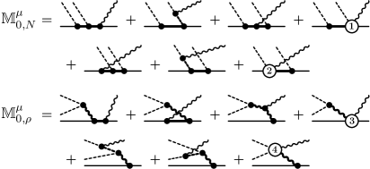
Figure 22: Explicit diagrams for two-pion photoproduction at the no-loop level, corresponding to Eq. (97), providing a full account of the topology inherent in the diagrams of Fig. 18. Internal thick lines subsume hadrons compatible with the reaction. Labels 1–4 indicate contact-type four-point currents. Depending on the level of sophistication, these diagrams indicate microscopic interaction currents incorporating two-body final-state interactions HNK06 or simple phenomenological contact currents. Details for the latter case are given in Appendix B.3. (For more discussion, see Sec. V.3.)

Hence, if all mechanisms depicted in these lowest-level diagrams are implemented fully, this requires dressing all vertices and propagators according to the description given in Sec. II.2 and, in particular, it requires accounting for all two-body final-state interactions in terms of contact-type four-point interaction currents (labeled by 1–4 in Fig. 22) such that local gauge invariance is preserved fully. This corresponds to full solutions of the underlying $\gamma N\to\pi N$ and $\gamma\rho\to\pi\pi$ problems at a level of sophistication that so far has never been undertaken because of the inherent nonlinearities of these problems. At their most sophisticated, such two-body subsystem dynamics are treated in linearized coupled-channel approaches that account for dressing and final-state effects. The two-pion production calculation reported in Ref. KJLMS09 , for example, corresponds to such an approximate treatment of the no-loop diagrams of Fig. 22 however, without properly accounting for gauge invariance. Moreover, no attempt was made to account for higher-order loops, thus effectively setting $\mathbb{R}^{\mu}=0$ in Eq. (96).

V.3.1 Tree-level approximation

At its most elementary, one may interpret the diagrams in Fig. 22 as tree-level diagrams, with Feynman propagators with physical masses, and vertices with physical coupling constants and phenomenological cutoff functions, based on effective Lagrangians. This is straightforward for the usual $s$-, $u$-, and $t$-channel diagrams of single-meson-production dynamics corresponding to diagrams like the correspondingly labeled ones from Figs. 1 and 7, for example. In fact, this is an approximation widely used in the literature for single-meson production. The preservation of local gauge invariance, however, demands that the corresponding contact-type interaction currents (labeled 1–4 in Fig. 22) be constructed in a manner that preserves local gauge invariance in terms of an off-shell generalized WTI. The advantages of proceeding in this way are threefold. First, the underlying single-meson production processes will of course be gauge invariant by construction. Second, and crucial for the present application, the two-meson production will be gauge invariant as well, without any additional work and the two contributing mechanisms $\mathbb{M}_{0,N}^{\mu}$ and $\mathbb{M}_{0,\rho}^{\mu}$ will be gauge invariant separately. Third, if one ever wishes to undertake the calculation of three or more meson-production processes based on the same elementary interaction mechanisms, the corresponding amplitudes will be gauge invariant as well. In other words, implementing local gauge invariance correctly at the lowest level will carry through to all levels of more complex dynamical situations.

Approximate treatments of interaction currents in terms of contact currents that preserve local gauge invariance have been suggested in Ref. HNK06 ; HHN11 and its variations have been used by a number of authors (including the present ones) in the study of one-meson photoproduction reactions HDHH12 ; NOH08 ; HHN12 . Explicit forms for the present application are given in Appendix B.3.

We mention that the majority of existing two-meson photo- and electroproduction models correspond to tree-level approximations of $\mathbb{M}^{\mu}_{0}$ of Eq. (97) with some variations. None of them includes the remainder current $\mathbb{R}^{\mu}$ and none preserve local gauge invariance, except Refs. NOH06 ; MON11 .

Before leaving this subsection, it should also be mentioned that while gauge invariance, analyticity, and covariance of the two-meson photo- and electroproduction are preserved in a tree-level approximation, unitarity is violated. Note that the origin of this kind of unitarity violation is different from that introduced by approximating the higher-order loop contributions of the $N\to\pi\pi N$ hadronic amplitude by a contact interaction as described in Sec. V.1.

VI Application to $\gamma N\to KK\Xi$

As a first application of the present formalism that will also allow us to assess the effect of accounting for higher-order loop contributions in terms of a phenomenological five-point current $\mathbb{R}^{\mu}$, we will calculate the $\gamma N\to KK\Xi$ reaction in the no-loop approximation of Eq. (96), with tree-level approximations for $\mathbb{M}_{0}^{\mu}$ as described in the preceding section. Here, we replace the produced two pions by two kaons and the nucleon in the final state by the cascade particle $\Xi$. For this particular reaction, the term equivalent to $\mathbb{M}_{0,\rho}^{\mu}$ in Eq. (97) is absent since the exchanged meson (the analog of the intermediate $\rho$ meson in Fig. 22) would need to have strangeness quantum number $|S|=2$ and no such meson has been observed so far. In summary, therefore, we employ the (approximate) description

$$M^{\mu}_{KK}=\mathbb{M}^{\mu}_{Y}+\mathbb{R}^{\mu}$$ (98)

for this process, where the topological structure of $\mathbb{M}^{\mu}_{Y}$ used here is given by the $\mathbb{M}^{\mu}_{0,N}$ group of diagrams in Fig. 22, with outgoing $\Xi$ baryon and intermediate hyperons $Y$.

To model the tree-level approximation to $\mathbb{M}^{\mu}_{Y}$, we basically follow Refs. NOH06 ; MON11 . The contributing intermediate states of the diagrams displayed in Fig. 22, in addition to kaons and ground-state baryons, also subsume other relevant mesons and baryon resonances, respectively. The four-point contact currents indicated by labels 1 and 2 in Fig. 22 used here are described in Appendix B.3. They differ from those employed in Refs. NOH06 ; MON11 by manifestly transverse contributions that do not affect gauge invariance, constructed along the lines of Eq. (125); in particular, see remarks below Eq. (126). For further details of the model for $\mathbb{M}^{\mu}_{Y}$, we refer to Refs. NOH06 ; MON11 . The main difference to those works is the inclusion here of an overall five-point remainder current $\mathbb{R}^{\mu}$ to approximately account for the effect of higher-order loops, as described in Sec. V.2. As a consequence, the free parameters of $\mathbb{M}^{\mu}_{Y}$ of Refs. NOH06 ; MON11 — especially, the coupling constants of the above-threshold resonances — are readjusted here to reproduce the $\Xi$ photoproduction data. The corresponding values are given in Table 1. All other parameter values are kept the same as given in Ref. MON11 .

Regarding the details for the remainder current $\mathbb{R}^{\mu}$, we note that the isospin structure (84) for the underlying $N\to KK\Xi$ vertex has separate contributions for isospins $T=0,\,1$ of the $K\Xi$ subsystem in the final state. This isospin structure carries over to the contact current $\mathbb{C}^{\mu}$ of Eq. (91), resulting in eight parameters $a^{T}_{i}$, $b^{T}_{i}$ ($i=1,\ldots,4$) for each isospin channel. Allowing for a parametric dependence on $s$, we make the ansatz

$$a^{T}_{i} =\tilde{a}^{T}_{i}\exp\left[-\alpha_{a}\left(\frac{s-s_{0}}{2m_{N}\Lambda_{S}}\right)^{2}\right]\left(\frac{s-s_{0}}{2m_{N}\Lambda_{S}}\right)^{2}~{},$$ (99a)

$$b^{T}_{i} =\tilde{b}^{T}_{i}\exp\left[-\alpha_{b}\left(\frac{s-s_{0}}{2m_{N}\Lambda_{S}}\right)^{2}\right]\left(\frac{s-s_{0}}{2m_{N}\Lambda_{S}}\right)^{2}~{},$$ (99b)

where $s\equiv(k+p)^{2}$ is the invariant mass of the reaction and $s_{0}\equiv(2m_{K}+m_{\Xi})^{2}$. The scale parameter $\Lambda_{S}$ is fixed at $\Lambda_{S}=1$ GeV. The constants $\tilde{a}^{T}_{i}$ and $\tilde{b}^{T}_{i}$, as well as $\alpha_{j}$ ($j=a,b$), are fit constants. For simplicity, we set $\alpha_{a}=\alpha_{b}$, and take $\tilde{a}_{i}$ and $\tilde{b}_{i}$ to be real in the present work. Furthermore, since at present there are data available only for the single charged channel corresponding to $\gamma p\to K^{+}K^{+}\Xi^{-}$, we set $a_{i}^{1}=b_{i}^{1}=0$ in the present application. These simplifications seem to be sufficient to reproduce the presently available data. The values obtained in our fits are given in Table 2.

Table 1: Adjusted parameter values entering $\mathbb{M}_{Y}^{\mu}$ of Eq. (98). All other parameter values are kept the same as given in Ref. MON11 .

Product of coupling constants	Values
$g_{N\Lambda K}g_{\Xi\Lambda K}$ for $\Lambda(1890)3/2^{+}$	$1.4$
$g_{N\Sigma K}g_{\Xi\Sigma K}$ for $\Sigma(2250)5/2^{-}$	$0.06$
$g_{N\Sigma K}g_{\Xi\Sigma K}$ for $\Sigma(2030)7/2^{+}$	$1.9$

Table 2: Fitted values of parameters $\tilde{a}_{i}^{T}$ and $\tilde{b}_{i}^{T}$ appearing in Eq. (99) for isospin channels $T=0,1$ of the outgoing $K\Xi$ subsystem. In this work, we set $\tilde{a}_{i}^{1}=\tilde{b}_{i}^{1}=0$ since only a single charged channel ($\gamma p\to K^{+}K^{+}\Xi^{-}$) is considered. Also, $\alpha_{a}=\alpha_{b}=2.4462$.

$i$	$\tilde{a}^{0}_{i}$ [fm]	$\tilde{b}^{0}_{i}$ [fm]
1	$8.4268$	$1.8314$
2	$1.5403$	$-1.6502$
3	$-2.3021$	$4.0460$
4	$-0.0014$	$1.4192$

For the present application, the single form factor $F$ we choose here for the hadronic $NKK\Xi$ vertex according to Eq. (85) is only needed in the context of having all external hadrons for the diagrams in Fig. 21 on their respective mass shells. Since for any of the corresponding kinematic situations only one of the intermediate hadrons is off-shell, effectively, without lack of generality, we may write the form factor as a separable product of functions in the form

$$F=f_{\Xi}(p^{\prime 2})f_{K}(q_{1}^{2})f_{K}(q_{2}^{2})f_{N}(p^{2})~{}.$$ (100)

Any form factor $F(p^{\prime 2},q_{1}^{2},q_{2}^{2};p^{2})$ can be reduced to this effective form within the present on-shell context. Following Refs. NOH06 ; MON11 , we employ

$$f_{K}(q^{2}) ={\frac{\Lambda_{K}^{2}-m_{K}^{2}}{\Lambda_{K}^{2}-q^{2}}}~{},$$ (101a)

$$f_{x}(p^{2}) =\frac{\Lambda_{x}^{4}}{\Lambda_{x}^{4}+(p^{2}-m_{x}^{2})^{2}}$$ (101b)

for the form factors entering the current $\mathbb{R}^{\mu}$, where $x=\Xi,\,N$, with associated masses $m_{x}$. As cutoff parameters, we choose $\Lambda_{\Xi}=\Lambda_{N}=900$ MeV and $\Lambda_{K}=1500$ MeV.

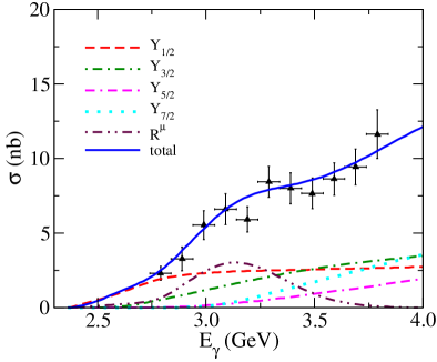
Figure 23: Total cross section for $\gamma p\to K^{+}K^{+}\Xi^{-}$ as a function of incident photon energy. The dashed (red) line corresponds to the spin-1/2 hyperons contribution; the dash-dotted (green) line to the spin-3/2 hyperons; the long-dashed (magenta) to spin-5/2 and dotted (cyan) to spin-7/2 resonance contributions. The long-dash-double-dotted (maroon) line corresponds to the phenomenological five-point current ($\mathbb{R}^{\mu}$) contribution. Data are from Ref. CLAS07b .

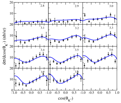
Figure 24: Differential cross section for $\gamma p\to K^{+}K^{+}\Xi^{-}$ as a function of $K^{+}$ emission angle in the center-of-mass system. Data are from Ref. CLAS07b .

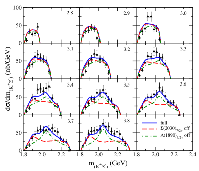
Figure 25: $K^{+}\Xi^{-}$ invariant-mass distribution in $\gamma p\to K^{+}K^{+}\Xi^{-}$, with full results shown as solid (blue) lines. The dashed (red) and dash-dotted (green) curves are obtained when the resonances $\Sigma(2030)7/2^{+}$ and $\Lambda(1890)3/2^{+}$, respectively, are switched off. Data are from Ref. CLAS07b .

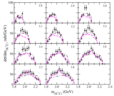
Figure 26: Effect of remainder current $\mathbb{R}^{\mu}$ on the $K^{+}\Xi^{-}$ invariant-mass distribution in $\gamma p\to K^{+}K^{+}\Xi^{-}$. The dashed (magenta) curves result from switching off the phenomenological remainder current $\mathbb{R}^{\mu}$ compared to the respective solid (blue) lines in Fig. 25. The dash-double-dotted (maroon) curves show the results of fitting the data using only the current $\mathbb{R}^{\mu}$ by itself. Data are from Ref. CLAS07b .

It should be noted that the parameterization (99) is minimal as far as reproducing the data is concerned, but by restricting $\tilde{a}_{i}$ and $\tilde{b}_{i}$ to be real, we manifestly violate unitarity. Similarly, in the hyperon resonance contributions entering in $\mathbb{M}^{\mu}_{Y}$ in the tree-level approximation, the associated coupling constants are also chosen to be real and the resonance widths are taken as constants ignoring their energy dependences. The presently available data (cross sections and invariant masses) are rather insensitive to these features of the parameters, unlike some of the spin observables which tend to be more sensitive to such details of the model. Given this situation and the fact that the detailed analysis of $\Xi$ photoproduction reaction is not the main objective of the present work, while in principle analytic properties from $S$-matrix theory should be imposed to improve upon the approximations employed in the present work, we defer such improvements to future studies dedicated to more detailed analyses once the corresponding database becomes more complete.

Figure 23 shows the total cross section results for the reaction $\gamma p\to K^{+}K^{+}\Xi^{-}$. The dynamical content of the present model is also displayed. We find that the spin-1/2 hyperons dominate at lower energies. The contribution of the remainder current $\mathbb{R}^{\mu}$, especially around $E_{\gamma}\approx 3.2$ GeV, is seen to be considerable. However, at this stage, it is not clear whether, as intended, the effect of $\mathbb{R}^{\mu}$ points to missing explicit higher-order contributions to provide a better resolution of detailed dynamics that produce the bump in the cross section (see also discussion below regarding Fig. 26) or whether it simply mimics possible hyperon resonance contributions not included in the present lowest-order model for $\mathbb{M}_{Y}^{\mu}$. In any case, from the values of the coupling constants given in Table 1, it is clear that the resonance content of the reaction is affected by the presence of $\mathbb{R}^{\mu}$ because the magnitudes of the strengths of the intermediate hyperons are now reduced compared to what was found in the previous model calculation MON11 (and the sign of the $\Sigma(2030)7/2^{+}$ coupling is changed as well). These are issues that remain to be investigated in future analyses when a more complete database becomes available.

The $K^{+}$ angular distribution in the center-of-mass frame of the system, displayed in Fig. 24, is reasonably well reproduced by the present model calculation. The effects of the above-threshold hyperon resonances on the $K^{+}\Xi^{-}$ invariant-mass distribution are shown in Fig. 25. We find that the $\Lambda(1890)3/2^{+}$ resonance contributes considerably, especially in the lower invariant-mass region, while the $\Sigma(2030)7/2^{+}$ resonance affects very much the higher invariant-mass region. Both resonances are crucial for reproducing the data, especially the $\Sigma(2030)7/2^{+}$. We note that the $\Sigma(2250)5/2^{-}$ resonance needed for reproducing a bump structure observed in the total cross section of the hadronic reaction $K^{-}p\to K^{+}\Xi^{-}$, as was shown in Ref. JOHN15 , is negligible for the present photoreaction $\gamma N\to KK\Xi$.

The effect of the remainder current $\mathbb{R}^{\mu}$ on the $K\Xi$ invariant mass is illustrated in Fig. 26. Switching off its contribution produces the dashed (magenta) curves. Comparing this with the full results shown in Fig. 25 reveals that the effect of $\mathbb{R}^{\mu}$ is substantial for energies in the range of $3.1<E_{\gamma}<3.4$ GeV, as discussed already in the context of the total cross section of Fig. 23. It should be pointed out that the remainder current $\mathbb{R}^{\mu}$ is important not just for improving the overall description of the total cross section, but for the differential cross section as well (the corresponding effect is not shown explicitly in Fig. 24). The dash-double-dotted (maroon) curves in the same figure show the results of fitting the $K^{+}\Xi$ invariant-mass data considering only the remainder current $\mathbb{R}^{\mu}$ by itself. (The fit was constrained by including total and differential cross-section data as well; the corresponding results are not shown here.) This clearly indicates the necessity to include some resonance contributions to reproduce the data.

We emphasize here that the present calculation does not exclude the possibility of other resonances contributing to these reaction processes. It simply reveals the most relevant resonances to describe the existing data. Clearly, to better constrain the choice of resonances, automatized penalty-based selection techniques, like the one recently described in Ref. LASSO18 , need to be implemented for future analyses. Moreover, for a more detailed analysis, it is strongly desirable to have more accurate data, especially, in the hadronic $\bar{K}N\to K\Xi$ process, where the currently existing data are of poor quality.

VII Summary and Discussion

Maintaining gauge invariance is trivial in any photo-process if all currents that contribute to the reaction are constructed in a manner that preserves their individual (generalized) Ward-Takahashi identities. The present considerations show that then putting together these currents in groups where each member can be related to the same topologically distinct hadronic process will not only imply gauge invariance for the entire group, but it will also ensure that this group as a whole will provide the correct four-divergence contribution if it appears as a subprocess within a larger and more complicated process. Consistency of the construction of the microscopic dynamics in terms of currents that satisfy off-shell WTIs is the key here. Mere current conservation alone does not help, because then one must start all over again when going over to a new problem. As a simple illustration of this point, let us consider the no-loop current given in Fig. 18. The fact that the four-point and two-point currents appearing in the graphs satisfy their respective off-shell WTIs automatically ensures gauge invariance of the NL currents. If, on the other hand, the construction of the single-pion photoproduction amplitude $M^{\mu}$ had been restricted to providing a conserved current only, and not the full off-shell WTI, the NL graphs of Fig. 18 would not be gauge invariant, and would not even provide a conserved current. In other words, one would need an additional unphysical mechanism to even construct a conserved current. Not considering at the outset the full set of diagrams that are needed for gauge invariance would make matters even worse.

With this microscopic consistency in mind, we have presented here a gauge-invariant theory for the production of two pions off the nucleon that applies equally well to real and virtual photons. The formalism is based on an extension of the field-theory approach of Ref. Haberzettl97 originally developed by one of the authors for single-pion photoproduction off the nucleon. In analogy to the single-pion case, we first constructed a complete description of the hadronic production process $N\to\pi\pi N$ by accounting for the multiple-scattering series of the interacting final $\pi\pi N$ system to all orders in terms of the Faddeev-type three-body AGS amplitudes AGS67 ; Sandhas72 . Coupling then the electromagnetic field to this hadronic system by employing the gauge derivative Haberzettl97 produced the closed-form expression of Eq. (46) for the full double-pion production current $M_{\pi\pi}^{\mu}$ that is gauge invariant as a matter of course. We emphasize in this respect the efficacy of the gauge-derivative procedure to identify and link all relevant reaction mechanisms in a microscopically consistent manner.

Most importantly for practical purposes, we have provided here a consistent expansion scheme for the full current in terms of groups of contributing currents that are easily identifiable by the topological complexity of the underlying hadronic processes and that are separately gauge invariant as a group. We have explicitly discussed in this manner the no-loop currents of Fig. 18 and the one-loop currents of Fig. 19.

Existing theoretical models based on baryon and meson degrees of freedom can all be subsumed under the no-loop scenario of Fig. 18, more explicitly depicted in Fig. 22. However, none of the models actually incorporates the full subsystem-process information in terms of, for example, the $\gamma N\to\pi N$ or the $\gamma\rho\to\pi\pi$ production currents which, as Fig. 22 clearly shows, would be necessary for a consistent description and which would be fairly straightforward to do given the technology available for treating such subprocesses in a gauge-invariant manner HBMF98a ; HNK06 ; HHN11 . As the details of Fig. 22 show, at the no-loop level practically all the theoretical effort needs to be expended on the adequate modeling of these subprocesses.

The situation is quite a bit more complicated at the two-loop level depicted in Fig. 19. Apart from the additional complication of the loop integrations itself and the fact that the meson-baryon and meson-meson amplitudes $X$ must be available, the most complicated ingredient in each of the three gauge-invariant groups of graphs is the occurrence of the interaction current $X^{\mu}$ for $\gamma\pi N\to\pi N$ in the two groups labeled 1L₁ and 1L₂, and for $\gamma\pi\pi\to\pi\pi$ in the 1L₃ group. Equation (20) shows that the interaction current $X^{\mu}$ itself is fairly complicated, requiring another double-loop integration for its full calculation, and it may not be possible to evaluate Eq. (20) in an actual application. However, in Appendix B.1 we provide a detailed, general description how any interaction current can be incorporated in a locally gauge-invariant manner by a phenomenological contact-type current. Local gauge invariance, therefore, need never be an issue even if other approximations may be necessary to render the problem manageable.

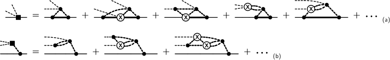
Figure 27: Hadronic two-pion production mechanism resulting from a three-pion vertex that start out as a four-body process until one of the mesons gets absorbed. The thick dashed and solid internal lines stand for any meson or baryon, respectively, compatible with the process. (a) Contact-type mechanisms summing up processes where at least one connection is made with the baryon line after the initial production. Part (b) sums up the three-body multiple-scattering series within the three-meson system, without intermediate reconnection with the baryon line. Once the final $\pi\pi N$ system occurs, subsequent interactions for both cases are topologically equivalent to that of the $\rho\pi\pi$ production vertex in Fig. 9(b) resulting in the graphs shown in Fig. 28. The contact-term contributions (a) are chosen to avoid double-counting with the mechanisms shown in Fig. 28.

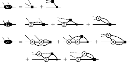
Figure 28: Higher-order double-pion-production contributions using the initial mechanisms depicted in Fig. 27. The no-loop (NL^′), one-loop (1L^′), and two-loop (2L^′) diagrams given here are exactly analogous to those of Fig. 11.

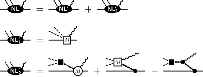
Figure 29: Current contributions resulting from the no-loop (NL^′) diagrams of Fig. 28. The four- and five-point currents indicated by square boxes labeled $M$ are given in Fig. 31.

The usefulness of an approximate treatment of neglected current contributions was demonstrated here for the reaction $\gamma N\to KK\Xi$ by describing the neglected higher-order loop contributions beyond the tree level in terms of a phenomenological remainder current $\mathbb{R}^{\mu}$. The results reported in Sec. VI show that despite the relative simplicity of the ansatz, the remainder current is indeed capable of contributing substantially to a good quantitative description of the reaction. In addition, the corresponding results point to where additional efforts need to be expended for a better description of the experimental data.

In deriving the present formalism, we have relied heavily on the dynamically correct formulation in terms of local gauge invariance because it provides a very convenient framework that allowed us to identify and consistently link in a straightforward manner all topologically relevant microscopic mechanisms. We emphasize, however, that as a consistent field-theory-based formulation, the resulting amplitudes satisfy as well the usual properties of Lorentz covariance and analyticity. With respect to unitarity, however, care must be exercised when approximating or truncating the full formalism, as mentioned in Secs. V.1 and V.3.1.

In summary, we have presented here a formulation of the two-pion production process off the nucleon based on field theory that is of the same level of rigor as the one-pion production described in Ref. Haberzettl97 . We hope that the present formulation of two-pion photoproduction will be of similar usefulness. Moreover, we emphasize that since the present formulation is based solely on the topological properties of the underlying hadronic production processes (cf. Fig. 9), it applies equally well to the photoproduction of any two mesons off any baryon resulting from topologically similar basic hadronic mechanisms.

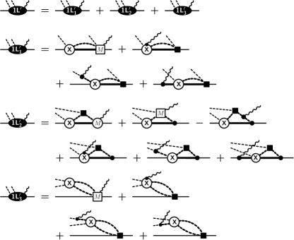
Figure 30: Current contributions resulting from the one-loop (1L^′) diagrams of Fig. 28. See Fig. 29 for details.

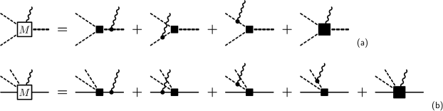
Figure 31: Two-pion photoproduction currents associated with (a) the effective two-pion vertex of Fig. 27(b) and (b) the contact vertex of Fig. 27(a). The respective last diagrams here (solid square boxes with photon attached) depict the four-point and five-point interaction currents of the respective processes.

Appendix A Incorporating four-meson vertices like $\omega\to\pi\pi\pi$

In this Appendix, we address the question how processes based on $n$-pion vertices for $n\geq 3$ can be incorporated into the formalism. As mentioned earlier, the dynamics resulting from such vertices requires at least a treatment in terms of an $(n+1)$-body problem. For the simplest possible case, e.g., the $\pi\pi\pi\omega$ vertex depicted in Fig. 9(c), this means that we need at least a four-body treatment. It is possible to do that in principle, i.e., the formalism for doing so exists GS67c ; Sandhas74 ; Sandhas75 ; AGS70 , but presumably there is little practical value to do so in full because of the enormous complexity of the relativistic version of that problem. Instead, we will take our cues from the full four-body problem of the $\pi\pi\pi N$ system and then reduce its complexity to a three-body problem by reabsorbing one of the mesons into either another meson or the nucleon, similar to the simple example depicted in Fig. 9(c).

Using the AGS four-body theory GS67c ; Sandhas74 ; Sandhas75 ; AGS70 , one finds two classes of graphs where the initial four-body system eventually is reduced to a three-body system because one of the three intermediate mesons is absorbed either in the baryon or another meson. If somewhere along the line before the final absorption at least one interaction with the baryon takes place, we find the processes depicted in Fig. 27(a), and if all scattering processes happen exclusively within the three-meson system, we obtain Fig. 27(b). We thus obtain a contact-type $\pi\pi NN$ vertex for Fig. 27(a) that behaves topologically like the sequential two-pion process of Fig. 9(a) where the intermediate nucleon propagation has shrunk to a point and an intermediate effective three-meson vertex for Fig. 27(b) that is topologically equivalent to the intermediate $\pi\pi\rho$ vertex of Fig. 9(b). Taken as effective “elementary” production processes, their resulting three-body dynamics is exactly like that of the basic processes depicted in Fig. 14, and we may apply the full formalism developed for them to the new effective two-pion production mechanisms of Fig. 27. Up to the two-loop level, therefore, we obtain the processes depicted in Fig. 28 which, apart from the fact that certain intermediate baryon lines have shrunk to a point, is completely analogous to Fig. 11.

Attaching the photon is now equally straightforward, producing the diagrams of Fig. 29 at the no-loop (NL^′) level and of Fig. 30 for the one-loop (1L^′) currents. Both sets of graphs are analogous to those of Figs. 18 and 19, respectively. The four- and five-point currents resulting from the mechanisms of Fig. 27 are given in Fig. 31. The crucial parts of these currents are the respective interaction currents (depicted as solid square boxes with an incoming photon attached) because formally they follow from coupling the photon to the respective interiors of the mechanisms depicted in Fig. 27 which in practice cannot be calculated such that the usual gauge-invariance constraints of an interaction current can be expected to hold true. However, as shown in the subsequent Appendix B, it is straightforward to find phenomenological approximations of these interaction currents that allow one to maintain the full off-shell gauge invariance of both currents in Fig. 31. The corresponding prescriptions for doing so consistently with whatever description one chooses for the underlying hadronic processes allowing for iterative refinements of approximations have been given in Ref. HNK06 , and there is no need here to repeat that discussion. In practical applications, therefore, one may employ phenomenological models for the two-pion production mechanisms in Fig. 27 without sacrificing gauge invariance. For the process in Fig. 31(b), in particular, we note that it is topologically equivalent to the remainder current $\mathbb{R}^{\mu}$ of Fig. 21. Therefore, if a meaningful approximate treatment of the contact-type hadronic process depicted in Fig. 27(a) can be extracted, one may use this as the basis for an approximate treatment along the lines outlined in Sec. V.2.

Figure 32: Examples of four-meson vertices producing three-body forces. There are several more examples of this kind.

The procedure just described takes care of two-pion systems evolving out of the initial four-body system created via a nucleon and a three-pion vertex. All subsequent interactions, however, follow the three-body dynamics described in Sec. III.1. To bring back the possibility of intermediate four-meson interactions, one may add any number of mechanisms involving four-meson vertices to the driving term (35) of the AGS equations. Some of the simplest examples are the three-body-force graphs shown in Fig. 32. Denoting such processes by $B_{\beta\gamma}$, one finds that the expansion of $M_{\beta}$ given in Eq. (40) then needs to be modified in lowest order as

$$M_{\beta}\to M^{\prime}_{\beta}=M_{\beta}+\sum_{\gamma,\alpha}B_{\beta\gamma}G_{0}X_{\gamma}G_{0}\bar{\delta}_{\gamma\alpha}F_{\alpha}+\cdots~{},$$ (102)

i.e., the additional terms are linear in $X_{\gamma}$, whereas the nonlinear mechanisms of Fig. 13 are of third order in $X_{\gamma}$. However, either one of such effects requires three-loop integrations at their respective lowest orders. For the graphs shown in Fig. 32, the extra term here corresponds to subjecting the final $\pi\pi N$ system of the one-loop graphs in Fig. 11 to the corresponding three-body forces.

We will not pursue this point any further since we suspect that it may be of limited practical value in view of the complexity of such mechanism. Also, for the same reason, we will not consider even more complex mechanisms with an even higher number of mesons produced at initial or intermediate stages. In any case, we would like to emphasize once more that, should the inclusion of more complicated mechanisms be deemed necessary for practical applications, the corresponding currents may simply be added without affecting gauge invariance of the existing approach because the currents of topologically independent hadronic graphs satisfy their own independent gauge-invariance constraints and this can be treated independently.

Appendix B Generalized contact currents

In this Appendix, we provide a generic expression for the phenomenological contact current describing the coupling of the photon to the interior interaction region of a hadronic transition process. Based on this general result, we will provide the full off-shell version of the five-point contact current for $\gamma N\to\pi\pi N$ whose on-shell form was provided in Sec. V.2 and the four-point contact currents used in the subprocesses of $\gamma N\to KK\Xi$ in Sec. VI.

The results follow by applying the gauge derivative introduced in Ref. Haberzettl97 as a formal way of applying minimal substitution to interacting systems. The resulting current will satisfy the appropriate generalized WTI (50) mandated by local gauge invariance Haberzettl97 . However, it may lack additional transverse current contributions that are required by additional physical constraints. Such transverse currents do not contribute to gauge invariance and thus are inaccessible to the gauge-derivative procedure. For contact currents, in particular, the gauge-derivative result needs to be amended by a manifestly transverse current to address the ‘violation of scaling problem’ at high energies DL72 . (The expressions presented here generalize the generic four-point-function results given in the appendix of Ref. HWH15 .)

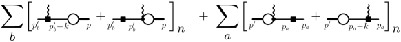
Figure 33: Schematic diagram corresponding to Eq. (109) for applying the gauge derivative to the $n$-th linearly independent contribution to the hadronic process (103). Sums over $b$ and $a$ enumerate contributions from the respective final and initial hadron legs to which a photon (wavy line) is attached. Solid squares depict coupling operators $G_{n}$ and open circles correspond to form factors $F_{n}$. Thick lines with momentum labels $p$ or $p^{\prime}$ generically stand for all incoming or outgoing legs, respectively. Lines labeled with momenta $p_{a}$ or $p^{\prime}_{b}$ indicate the particle to which the photon couples; all other particle lines (incoming or outgoing) not participating in the electromagnetic interaction are omitted for clarity. The photon carries a momentum $k$ into the process, i.e., all downstream momenta are accordingly increased. Overall, the initial and final momentum sets $p$ and $p^{\prime}$, respectively, are fixed and satisfy (108); only the internal momenta can increase ($p_{a}+k$) or decrease ($p^{\prime}_{b}-k$) accordingly.

B.1 Contact current for arbitrary hadronic transition

An arbitrary hadronic transition process for $N_{i}$ incoming hadrons going over to $N_{f}$ outgoing hadrons may generically be written as

$$\mathbb{F}=\sum_{n}G_{n}F_{n}$$ (103)

where the sum extends over all linearly independent operator structures $G_{n}$ and (complex) scalar functions $F_{n}$. An example of this would be the structure given in Eq. (83) for $N\to\pi\pi N$, but generically this applies also to any other transition like $N\to\pi N$, $\rho\to\pi\pi$, $NN\to NN$, etc. (The latter contact currents are needed for bremsstrahlung NH09 ; HN10 .)

In general, assuming four-momentum conservation, the form factors $F_{n}$ depend on the $(N_{i}+N_{f})(N_{i}+N_{f}-1)/2$ scalar invariants one can form from the $N_{i}+N_{f}-1$ independent particle momenta. Without lack of generality, they may all be written as squares of individual momenta, or as squares of sums or differences of two momenta, and we may always choose the set of all $N_{i}+N_{f}$ squares of external momenta to be among the squares necessary for a complete description of the specific dynamical situation described by $F_{n}$. As we shall see by construction in the following, limiting our discussion in the following to this subset of squared momenta will be sufficient for the present phenomenological purposes.

In the following, incoming and outgoing hadron momenta will be, respectively, unprimed, $p_{a}$, and enumerated by index $a=1,\ldots,N_{i}$, and primed, $p^{\prime}_{b}$, and enumerated by index $b=1,\dots,N_{f}$.

Hence, for the present phenomenological purpose, we assume that the form factors $F_{n}$ depend only on the squares of all incoming and outgoing hadronic momenta $p_{a}^{2}$ and $p^{\prime 2}_{b}$, respectively, i.e.,

$$F_{n}=F_{n}(p^{\prime 2}_{1},\ldots,p^{\prime 2}_{N_{f}};p^{2}_{1},\ldots,p^{2}_{N_{i}})~{},$$ (104)

ignoring other possible squares like $(p^{\prime}_{b}-p_{a})^{2}$, etc. In general, we allow for off-shell momenta, but four-momentum conservation,

$$\sum_{a}p_{a}=\sum_{b}p^{\prime}_{b}~{},$$ (105)

is always assumed. Note that we suppress here the isospin structure in (103) because it has no bearing on the basic approach. (However, isospin dependence will give rise to the charge parameters $e_{x}$ below associated with legs of external particles $x$.)

When applying the gauge derivative Haberzettl97 , it will act on four-momenta in both coupling $G_{n}$ operators and form factors $F_{n}$. In general, if depending on momenta, $G_{n}$ may depend on arbitrary powers of the momentum of a particular particle leg and it may depend on products of momenta from different legs. When applying the gauge derivative to such products, they need to be treated according to the usual product rule for derivatives. However, regarding the photon coupling to a particular leg, the momentum dependence arising from other legs is irrelevant, in other words, the gauge derivative effectively acts like a partial derivative that affects only the momentum of the active leg. Furthermore, we need to account for whether that momentum pertains to an incoming leg or an outgoing leg.

The contact current,

$$\mathbb{C}^{\mu} =-\{\mathbb{F}\}^{\mu}+\mathbb{T}^{\,\mu}$$

$$=\sum_{n}\left[-\{G_{n}F_{n}\}^{\mu}+G_{n}\mathbb{T}^{\,\mu}_{n}\right],$$ (106)

associated with coupling a photon (with Lorentz index $\mu$) to the interior of the process $\mathbb{F}$ is obtained by applying the gauge derivative $\{\cdots\}^{\mu}$ here Haberzettl97 and adding a judiciously constructed manifestly transverse current $\mathbb{T}^{\mu}=\sum_{n}G_{n}\mathbb{T}_{n}$ to avoid the high-energy scaling violation discussed by Drell and Lee DL72 . The gauge derivative results in

$$\{G_{n}F_{n}\}^{\mu} =\left\{G_{n}\,F_{n}\right\}^{\mu}_{\text{out}}+\left\{F_{n}\,G_{n}\right\}^{\mu}_{\text{in}}$$

$$=\sum_{b}\left[\big{\{}G^{(b)}_{n}\big{\}}^{\mu}_{b}F_{n}+G^{(b)}_{n}\big{\{}F_{n}\big{\}}^{\mu}_{b}\right]$$

$$\quad\mbox{}+\sum_{a}\left[\big{\{}F_{n}\big{\}}^{\mu}_{a}G_{n}^{(a)}+F_{n}\big{\{}G_{n}^{(a)}\big{\}}^{\mu}_{a}\right]~{},$$ (107)

where the terms are ordered here according to where couplings occur during the reaction, with the couplings containing outgoing momenta (sum over $b$), denoted by $G_{n}^{(b)}$, placed on the left and couplings containing incoming momenta (sum over $a$), denoted by $G_{n}^{(a)}$, placed on the right. The ordering is necessary to properly account for the fact that the momentum $k$ carried into the reaction by the photon is available only for particles downstream of the photon coupling. Diagrammatically, this is depicted in Fig. 33. With four-momenta of all external particles taking part in the photoprocess at their fixed values, with four-momentum conservation,

$$\sum_{a}p_{a}+k=\sum_{b}p^{\prime}_{b}~{},$$ (108)

we obtain

$$\{G_{n}F_{n}\}^{\mu} =\sum_{b}\bigg{[}\left\{G_{n}^{(b)}(p^{\prime}_{b}-k)\right\}^{\mu}F_{n}^{(b)}\big{(}(p^{\prime}_{b}-k)^{2}\big{)}$$

$$\qquad\qquad\mbox{}+G_{n}^{(b)}(p^{\prime}_{b})\left\{F_{n}^{(b)}\big{(}(p^{\prime}_{b}-k)^{2}\big{)}\right\}^{\mu}\bigg{]}$$

$$\mbox{}\quad+\sum_{a}\bigg{[}\left\{F_{n}^{(a)}\big{(}p_{a}^{2}\big{)}\right\}^{\mu}G_{n}^{(a)}(p_{a})$$

$$\qquad\qquad\mbox{}+F_{n}^{(a)}\big{(}(p_{a}+k)^{2}\big{)}\left\{G_{n}^{(b)}(p_{a})\right\}^{\mu}\bigg{]}~{},$$ (109)

where the four terms under the sums and their momenta are shown in Fig. 33. The notation $F_{n}^{(b)}\big{(}(p^{\prime}_{b}-k)^{2}\big{)}$ means that all hadron legs carry the momentum appropriate for the photo process, except the outgoing particle $b$, which has $p^{\prime}_{b}-k$ to ensure four-momentum conservation across the hadronic process. Similarly for $F_{n}^{(a)}\big{(}(p_{a}+k)^{2}\big{)}$, all momenta are fixed at their external values, except for the particle $a$ coming into the hadronic process after it has interacted with the photon and thus has $p_{a}+k$.

The gauge derivatives of the coupling operators,

$$\Gamma^{\mu}_{n,b} \equiv-\left\{G_{n}^{(b)}(p^{\prime}_{b}-k)\right\}^{\mu}~{},$$ (110a)

$$\Gamma^{\mu}_{n,a} \equiv-\left\{G_{n}^{(a)}(p_{a})\right\}^{\mu}~{},$$ (110b)

provide Kroll-Ruderman-type (KRt) photon couplings arising from the hadronic coupling operators independent of any form-factor dependence. When evaluating these gauge derivatives, only the momenta of respective outgoing and incoming particles $b$ and $a$ are contributing. An example of such KRt couplings is furnished by the $\gamma^{\mu}$ couplings in Eq. (142) for $\gamma NN\pi\pi$. The details of such couplings depend on a particular application, but, in general, their four-divergences are given by

$$k_{\mu}\Gamma_{n,b}^{\mu} =e_{b}\left[G_{n}^{(b)}(p^{\prime}_{b}-k)-G_{n}^{(b)}(p^{\prime}_{b})\right]~{},$$ (111a)

$$k_{\mu}\Gamma_{n,a}^{\mu} =e_{a}\left[G_{n}^{(a)}(p_{a})-G_{n}^{(a)}(p_{a}+k)\right]~{},$$ (111b)

where the parameters $e_{b}$ and $e_{a}$ describe the charges of particles $b$ and $a$, respectively. These results are essential for deriving the four-divergence of the contact current $\mathbb{C}^{\mu}$ given in Eq. (124) below. Note that their structure at the elementary level of a single particle leg is the same as the general result (50) for interaction currents. The subsequent Sec. B.1.1 will provide further discussion of elementary gauge derivatives needed for evaluating the KRt currents (110) and a proof of Eqs. (111).

To evaluate the action of coupling the photon to the form factors in (109), we note that using the elementary gauge derivative $\{q^{2}\}^{\mu}=Q(2q+k)^{\mu}$ for a particle of momentum $q$ with charge $Q$, one can easily show that the gauge derivative of a scalar function $f(q^{2})$ associated with that particle is given by

$$\left\{f(q^{2})\right\}^{\mu}=Q(q^{\prime}+q)^{\mu}\frac{f(q^{\prime 2})-f(q^{2})}{q^{\prime 2}-q^{2}}~{},$$ (112)

where $q^{\prime}=q+k$ is the particle’s momentum after the electromagnetic interaction. This has the structure of a manifestly nonsingular finite-difference derivative. (This is an exact result, not a phenomenological ansatz.) For the following, it will be useful to introduce abbreviations

$$s_{a}=(p_{a}+k)^{2}\quad\text{and}\quad u_{b}=(p^{\prime}_{b}-k)^{2}$$ (113)

for Mandelstam-like squares associated with initial and final momenta, respectively, to express some of the squared momenta appearing here.

Straightforward algebra shows now that the full contact current (106) may be written as

$$\mathbb{C}^{\mu}=\sum_{n}\Big{[}\mathbb{K}^{\mu}_{n}+G_{n}(\mathbb{S}^{\mu}_{n}+\mathbb{T}^{\mu}_{n})\Big{]}~{},$$ (114)

where

$$\mathbb{K}^{\mu}_{n}=\sum_{b}\Gamma^{\mu}_{n,b}\,F_{n}^{(b)}(u_{b})+\sum_{a}\Gamma^{\mu}_{n,a}\,F_{n}^{(a)}(s_{a})$$ (115)

subsumes the contributions from the KRt electromagnetic couplings (110) to the initial and final four-momenta in the hadronic coupling operator $G_{n}$. The scalar finite-difference coupling (112) to the form factors then produces the current $\mathbb{S}^{\,\mu}_{n}$. Adding a transverse current $\mathbb{T}^{\,\mu}_{n}$, to be discussed presently, we may write

$$\mathbb{S}^{\,\mu}_{n}+\mathbb{T}^{\,\mu}_{n} =-\sum_{b}e_{b}(2p^{\prime}_{b}-k)^{\mu}\frac{F_{n}^{(b)}(u_{b})-\hat{F}_{n}+\hat{F}_{n}H_{n}}{u_{b}-p^{\prime 2}_{b}}$$

$$\quad\mbox{}-\sum_{a}e_{a}(2p_{a}+k)^{\mu}\frac{F_{n}^{(a)}(s_{a})-\hat{F}_{n}+\hat{F}_{n}H_{n}}{s_{a}-p^{2}_{a}}$$

$$=-\sum_{b}e_{b}(2p^{\prime}_{b}-k)^{\mu}\frac{F_{n}^{(b)}(u_{b})-\hat{F}_{n}}{u_{b}-p^{\prime 2}_{b}}\,H_{n}^{(b)}$$

$$\quad\mbox{}-\sum_{a}e_{a}(2p_{a}+k)^{\mu}\frac{F_{n}^{(a)}(s_{a})-\hat{F}_{n}}{s_{a}-p^{2}_{a}}\,H_{n}^{(a)}~{},$$ (116)

where $H_{n}$ is the dimensionless function:

$$H_{n}=\prod_{b}\left[1-\delta_{b}\frac{F_{n}^{(b)}(u_{b})}{\hat{F}_{n}}\right]\prod_{a}\left[1-\delta_{a}\frac{F_{n}^{(a)}(s_{a})}{\hat{F}_{n}}\right]~{},$$ (117)

with $\delta_{x}=1$ (for $x=b,a$) if particle $x$ carries charge; otherwise it is zero. The function $\hat{F}_{n}$ is given by

$$\hat{F}_{n}=F_{n}(p^{\prime 2}_{1},\ldots,p^{\prime 2}_{N_{f}};p^{2}_{1},\ldots,p^{2}_{N_{i}})~{},$$ (118)

which is an unphysical value of $F_{n}$ because its momenta here are related by Eq. (108), and not by Eq. (105). The function $H_{n}$ thus vanishes whenever any of the denominators in Eq. (116) vanishes, thus rendering Eq. (116) manifestly nonsingular. The functions $H^{(b)}_{n}$ and $H^{(a)}_{n}$ are obtained by removing one of the factors from $H_{n}$ resulting in

$$H_{n}^{(b)} =1-\frac{\hat{F}_{n}H_{n}}{\hat{F}_{n}-\delta_{b}F_{n}^{(b)}(u_{b})}=\sum_{b^{\prime}\neq b}\delta_{b^{\prime}}F_{n}^{(b^{\prime})}(u_{b^{\prime}})+\cdots~{},$$ (119a)

$$H_{n}^{(a)} =1-\frac{\hat{F}_{n}H_{n}}{\hat{F}_{n}-\delta_{a}F_{n}^{(a)}(s_{a})}=\sum_{a^{\prime}\neq a}\delta_{a^{\prime}}F_{n}^{(a^{\prime})}(s_{a^{\prime}})+\cdots~{}.$$ (119b)

The right-most expressions here show that the leading fall-off behavior at large energies is that of the form factors; explicit expressions for higher orders are omitted here.

The transverse current $\mathbb{T}_{n}^{\mu}$ in Eq. (116) arises solely from the sum of terms proportional to $H_{n}$. In other words, the four-divergence of

$$\mathbb{T}^{\mu}_{n}=-\bigg{[}\sum_{b}e_{b}\frac{(2p^{\prime}_{b}-k)^{\mu}}{u_{b}-p^{\prime 2}_{b}}+\sum_{a}e_{a}\frac{(2p_{a}+k)^{\mu}}{s_{a}-p^{2}_{a}}\bigg{]}\hat{F}_{n}H_{n}$$ (120)

vanishes identically,

$$k_{\mu}\mathbb{T}^{\mu}\equiv 0~{},$$ (121)

because of charge conservation,

$$\sum_{b}e_{b}=\sum_{a}e_{a}~{}.$$ (122)

However, it is this transverse current that leads to the factors $H_{n}^{(b)}$ and $H_{n}^{(b)}$ in Eq. (116) providing the necessary high-energy fall-off behavior to prevent the violation of scaling discussed in Ref. DL72 . Without this transverse current (i.e., for $H_{n}\equiv 0$), these factors would all be unity. This limit defines $\mathbb{S}^{\mu}_{n}$, which therefore by itself provides the full four-divergence of Eq. (116),

$$k_{\mu}\mathbb{S}^{\mu}_{n}=\sum_{b}e_{b}F_{n}^{(b)}(u_{b})-\sum_{a}e_{a}F_{n}^{(a)}(s_{a})~{}.$$ (123)

Note here that this result would correspond to the complete generalized WTI of Eq. (50) for scalar coupling, where $G_{n}$ is a constant and $\mathbb{K}^{\mu}_{n}\equiv 0$. For bare particles, with a constant value for the form factors, this four-divergence vanishes because of charge conservation (122).

It is now a simple exercise to verify that the full contact current $\mathbb{C}^{\mu}$ given by the general expression (114) satisfies

$$k_{\mu}\mathbb{C}^{\mu} =\sum_{b}e_{b}\left(\sum_{n}G^{(b)}_{n}(p^{\prime}_{b}-k)F^{(b)}_{n}(u_{n})\right)$$

$$\qquad\mbox{}-\sum_{a}e_{a}\left(\sum_{n}G^{(a)}_{n}(p_{a}+k)F_{n}^{(a)}(s_{a})\right)~{},$$ (124)

where the sums in the parentheses provide different kinematical situations for $\mathbb{F}$ of Eq. (103), with all external four-momenta fixed at the values appropriate for the photoprocess except for particles $b$ and $a$ in the sums which respectively have four-momenta $p^{\prime}_{b}-k$ and $p_{a}+k$ so that the photoprocess four-momentum conservation (108) holds true. The four-divergence (124) thus corresponds to Eq. (50) proving that $\mathbb{C}^{\mu}$ is indeed a locally gauge-invariant contact current.

The construction presented here for $\mathbb{C}^{\mu}$ of Eq. (114) is the minimal result that satisfies all constraints. However, regarding the full dynamics of a contact-type interaction current, in general there may be additional transverse contributions that cannot be determined uniquely by the gauge-derivative procedure and thus require a more detailed microscopic calculation. We emphasize, however, that the gauge derivative will identify and consistently link all contributing topologically distinct reactions mechanisms even if the explicit electromagnetic coupling operator may be subject to transversality ambiguities (cf. subsequent Sec. B.1.1). As a case in point, we mention the transverse treatment of final-state interactions for the $\gamma N\to\pi N$ reaction in Ref. HNK06 .

In principle, from a phenomenological point of view, one may add terms to the right-hand side of Eq. (114), as long as they are transverse, nonsingular, fall off fast enough at high energies as to not violate scaling DL72 , and are independent of individual particle indices. The manifestly transverse expression

$$\textbf{T}^{\mu}_{n}=\left[\boldsymbol{\Gamma}^{\mu}_{n}\left(\mathbb{S}^{\,\nu}_{n}+\mathbb{T}^{\,\nu}_{n}\right)-\boldsymbol{\Gamma}^{\,\nu}_{n}\left(\mathbb{S}^{\mu}_{n}+\mathbb{T}^{\mu}_{n}\right)\right]k_{\nu}$$ (125)

satisfies all of these constraints for any well-behaved current operator $\boldsymbol{\Gamma}^{\mu}_{n}$. To be consistent within the present approach this operator should be based on the KRt currents (110), leading to the ansatz

$$\boldsymbol{\Gamma}^{\mu}_{n}=\sum_{a}\hat{\Gamma}^{\mu}_{n,a}-\sum_{b}\hat{\Gamma}^{\mu}_{n,b}~{},$$ (126)

where $\hat{\Gamma}^{\mu}_{n,x}$ is equal to $\Gamma^{\mu}_{n,x}$ with charge $e_{x}$ replaced by $\delta_{x}$ (for $x=b,a$). With this choice, Eq. (125) provides the simplest additional transverse current that treats contributions from incoming and outgoing particle legs on an equal footing and utilizes only dynamical elements that are already part of the current $\mathbb{C}^{\mu}$. Thus, in phenomenological approaches one may exploit these features and add linear combinations $\textbf{T}^{\mu}=\sum_{n}c_{n}\textbf{T}^{\mu}_{n}$, with (dimensionless) fit parameters $c_{n}$, without affecting gauge invariance. This basically readjusts the form-factor weights for each KRt coupling in Eq. (115) and the overall hadronic coupling operator $G_{n}$ for the auxiliary current $\mathbb{S}^{\nu}_{n}+\mathbb{T}^{\nu}_{n}$ in a gauge-invariant manner. We mention in this context that the four-point contact currents given in Refs. NOH06 ; MON11 utilize this freedom, corresponding to coefficients $c_{n}=1$ (with $n=1$).

B.1.1 Proof of Eqs. (111)

For the proof of Eqs. (111), we will only discuss the currents $\Gamma^{\mu}_{n,a}$ for incoming particles $a$; the proof for outgoing particles $b$ can then easily be found along the same lines. Thus, suppressing all extraneous indices, we shall prove that

$$\Gamma^{\mu}=-\{G(p)\}^{\mu}$$ (127)

implies

$$k_{\mu}\Gamma^{\mu}=Q\left[G(p)-G(p+k)\right]~{},$$ (128)

where $G(p)$ is the relevant hadronic coupling operator of the (incoming) particle with charge $Q$ and momentum $p$.

If $G(p)$ is a constant or linear in the momentum, the result follows trivially because the gauge derivative of a constant vanishes, and if it is linear in the momentum, there are only two possibilities Haberzettl97 ,

$$\left\{p^{\nu}\right\}^{\mu}=Qg^{\mu\nu}\qquad\text{and}\qquad\left\{\not{p}\right\}^{\mu}=Q\gamma^{\mu}~{},$$ (129)

which both satisfy (128). The KRt currents in Eq. (142) of the subsequent Sec. B.2 are of this simple kind. The situation is more complicated if the coupling is of a higher order because the gauge derivative is not unique for such cases; it depends on the order of the (commuting) factors since factors downstream (i.e., to the left) of the gauge-derivative action acquire the extra photon momentum $k$. For example, the expressions

$$\left\{p^{\lambda}p^{\nu}\right\}^{\mu} =Q\left[g^{\mu\lambda}p^{\nu}+(p+k)^{\lambda}g^{\mu\nu}\right]~{},$$ (130a)

$$\left\{p^{\nu}p^{\lambda}\right\}^{\mu} =Q\left[g^{\mu\nu}p^{\lambda}+(p+k)^{\nu}g^{\mu\lambda}\right]$$ (130b)

differ by a manifestly transverse term. Such transverse terms have no bearing on gauge invariance and may be ignored for the present discussion. (Of course, they may be quite relevant for the physics of a given problem.) In general, choosing any particular order for higher-order momentum dependences will be subject to such transversality ambiguities. One may choose to deal with this ambiguity in a democratic fashion by symmetrizing the expression, i.e.,

$$\frac{1}{2}\left\{p^{\lambda}p^{\nu}+p^{\nu}p^{\lambda}\right\}^{\mu}=\frac{Q}{2}\left[g^{\mu\lambda}(2p+k)^{\nu}+g^{\mu\nu}(2p+k)^{\lambda}\right]~{},$$ (131)

because this treats all factors on an equal footing. (Moreover, it will provide current expressions that are symmetric in $p$ and $p^{\prime}=p+k$, which clearly is desirable.) This is easy to do for two factors like $p^{\lambda}p^{\nu}$ here or $\not{p}p^{\nu}$, etc. For either one of such cases one may easily show explicitly that Eq. (128) is true irrespective of the chosen order, whether one symmetrizes or not.

For higher orders of coupling that may occur for higher-spin particles, there are $m!$ ordering possibilities for $m$ momentum factors. However, for the purpose of the proof, there is no need to consider symmetrization explicitly. We may just take one arbitrary order, number the factors from right to left, and write

$$G(p)=f_{m}(p)f_{m-1}(p)\ldots f_{n+1}(p)f_{n}(p)\ldots f_{1}p)~{},$$ (132)

where each factor here is linear in $p$. Since we know that Eq. (128) is true for linear and quadratic couplings, we may now prove that it is true for $G(p)$ by induction assuming that it is true for

$$G_{n}(p)=f_{n}(p)\ldots f_{1}p)$$ (133)

and show that it remains true for

$$G_{n+1}(p)=f_{n+1}(p)\,G_{n}(p)~{}.$$ (134)

Using the product rule, the gauge derivative for $n+1$ coupling factors is given as

$$\Gamma^{\mu}_{n+1} \equiv-\left\{G_{n+1}(p)\right\}^{\mu}$$

$$=-\left\{f_{n+1}(p)\right\}^{\mu}G_{n}(p)-f_{n+1}(p+k)\left\{G_{n}(p)\right\}^{\mu}~{}.$$ (135)

With

$$-k_{\mu}\left\{f_{n+1}(p)\right\}^{\mu}=Q\left[f_{n+1}(p)-f_{n+1}(p+k)\right]$$ (136)

and

$$-k_{\mu}\left\{G_{n}(p)\right\}^{\mu}=Q\left[G_{n}(p)-G_{n}(p+k)\right]$$ (137)

as stipulated, we then immediately find upon taking the four-divergence of (135) and inserting these expressions that indeed

$$k_{\mu}\Gamma^{\mu}_{n+1} =Q\left[G_{n+1}(p)-G_{n+1}(p+k)\right]~{},$$ (138)

which proves (128) for $n+1$ factors. Thus, letting $n+1$ go to $m$ proves the assertion.

It should be obvious now that this will remain true for a fully symmetrized KRt current since each of the $m!$ current terms in the sum will yield the same expression (128). Dividing then by $m!$ to properly normalize the current shows that Eq. (128) also holds true for the symmetrized version.

B.2 Five-point contact current for $\gamma N\to\pi\pi N$

The generic expressions of the previous section will now be applied to generalize the phenomenological five-point contact current for $\gamma N\to\pi\pi N$ provided in Sec. V.2. The most general phenomenological ansatz for the hadronic $\pi\pi NN$ vertex (83) is given by

$$\mathbb{C}(p^{\prime},q_{1},q_{2};p) =a_{1}F_{1}+a_{2}\frac{\not{p}}{m}F_{2}+a_{3}\frac{\not{p}^{\prime}}{m^{\prime}}F_{3}+a_{4}\frac{\not{p}^{\prime}\not{p}}{m^{\prime}m}F_{4}$$

$$\quad\mbox{}+b_{1}\frac{\not{q}}{m_{\pi}}F_{5}+b_{2}\frac{\not{q}\not{p}}{m_{\pi}m}F_{6}+b_{3}\frac{\not{p}^{\prime}\not{q}}{m^{\prime}m_{\pi}}F_{7}$$

$$\quad\mbox{}+b_{4}\frac{\not{p}^{\prime}\not{q}\not{p}}{m^{\prime}m_{\pi}m}F_{8}$$ (139)

in terms of eight phenomenological form factors,

$$F_{i}=F_{i}(p^{\prime 2},q_{1}^{2},q_{2}^{2};p^{2})~{},\quad\text{for}\quad i=1,\ldots,8~{},$$ (140)

instead of the one of Eq. (85), with fit constants $a_{j}$, $b_{j}$ ($j=1,\ldots,4$) for the eight independent coupling operators. [We suppress here the isospin dependence (84) of the vertex which will double the number of fit parameters; see Sec. VI.] The momenta here are defined as in Eq. (82).

Following the previous section, the associated contact current may be written as

$$\mathbb{C}^{\mu} =\mathbb{K}^{\mu}+a_{1}C^{\mu}_{1}+a_{2}\frac{\not{p}}{m}C^{\mu}_{2}+a_{3}\frac{\not{p}^{\prime}}{m^{\prime}}C^{\mu}_{3}$$

$$\quad\mbox{}+a_{4}\frac{\not{p}^{\prime}\not{p}}{m^{\prime}m}C^{\mu}_{4}+b_{1}\frac{\not{q}}{m_{\pi}}C^{\mu}_{5}+b_{2}\frac{\not{q}\not{p}}{m_{\pi}m}C^{\mu}_{6}$$

$$\quad\mbox{}+b_{3}\frac{\not{p}^{\prime}\not{q}}{m^{\prime}m_{\pi}}C^{\mu}_{7}+b_{4}\frac{\not{p}^{\prime}\not{q}\not{p}}{m^{\prime}m_{\pi}m}C^{\mu}_{8}~{},$$ (141)

where the Dirac structure of the coupling operators in (139) gives rise to 16 KRt contributions

$$\mathbb{K}^{\mu} =-e_{i}\Big{[}a_{2}\frac{\gamma^{\mu}}{m}F_{2,i}+a_{4}\frac{\not{p}^{\prime}\gamma^{\mu}}{m^{\prime}m}F_{4,i}$$

$$\qquad\qquad\mbox{}+b_{2}\frac{\not{q}\gamma^{\mu}}{m_{\pi}m}F_{6,i}+b_{4}\frac{\not{p}^{\prime}\not{q}\gamma^{\mu}}{m^{\prime}m_{\pi}m}F_{8,i}\Big{]}$$

$$\quad\mbox{}-e_{f}\Big{[}a_{3}\frac{\gamma^{\mu}}{m^{\prime}}F_{3,f}+a_{4}\frac{\gamma^{\mu}\not{p}}{m^{\prime}m}F_{4,f}$$

$$\qquad\qquad\mbox{}+b_{3}\frac{\gamma^{\mu}\not{q}}{m^{\prime}m_{\pi}}F_{7,f}+b_{4}\frac{\gamma^{\mu}\not{q}\not{p}}{m^{\prime}m_{\pi}m}F_{8,f}\Big{]}$$

$$\quad\mbox{}-e_{1}\Big{[}b_{1}\frac{\gamma^{\mu}}{m_{\pi}}F_{5,1}+b_{2}\frac{\gamma^{\mu}\not{p}}{m_{\pi}m}F_{6,1}$$

$$\qquad\qquad\mbox{}+b_{3}\frac{\not{p}^{\prime}\gamma^{\mu}}{m^{\prime}m_{\pi}}F_{7,1}+b_{4}\frac{\not{p}^{\prime}\gamma^{\mu}\not{p}}{m^{\prime}m_{\pi}m}F_{8,1}\Big{]}$$

$$\quad\mbox{}+e_{2}\Big{[}b_{1}\frac{\gamma^{\mu}}{m_{\pi}}F_{5,2}+b_{2}\frac{\gamma^{\mu}\not{p}}{m_{\pi}m}F_{6,2}$$

$$\qquad\qquad\mbox{}+b_{3}\frac{\not{p}^{\prime}\gamma^{\mu}}{m^{\prime}m_{\pi}}F_{7,2}+b_{4}\frac{\not{p}^{\prime}\gamma^{\mu}\not{p}}{m^{\prime}m_{\pi}m}F_{8,2}\Big{]}~{}.$$ (142)

The parameters $e_{i}$, $e_{f}$, $e_{1}$, and $e_{2}$ are the individual charges of the incoming and outgoing nucleons and the two pions related by charge conservation,

$$e_{1}+e_{2}+e_{f}=e_{i}~{}.$$ (143)

The functions $F_{j,x}$, for $j=1,\ldots,8$, are defined by

$$F_{j,i} =F_{j}(p^{\prime 2},q^{2}_{1},q^{2}_{2};s)~{},$$ (144a)

$$F_{j,f} =F_{j}(u,q^{2}_{1},q^{2}_{2};p^{2})~{},$$ (144b)

$$F_{j,1} =F_{j}(p^{\prime 2},t_{1},q^{2}_{2};p^{2})~{},$$ (144c)

$$F_{j,2} =F_{j}(p^{\prime 2},q^{2}_{1},t_{2};p^{2})~{},$$ (144d)

with Mandelstam-type variables

$$s=(p+k)^{2}~{},\qquad u=(p^{\prime}-k)^{2}$$ (145)

for the nucleons and

$$t_{1}=(q_{1}-k)^{2}~{},\qquad t_{2}=(q_{2}-k)^{2}$$ (146)

for the pions. The indices $x=i,f,1,2$, therefore, serve as reminders of the kinematic situations of intermediate off-shell hadrons in the first four diagrams labeled $\mathbb{R}^{\mu}_{x}$ in Fig. 21.

The eight auxiliary scalar contact currents $C^{\mu}_{j}$, for $j=1,\dots,8$, follow from Eq. (116) as

$$C^{\mu}_{j} =-e_{1}(2q_{1}-k)^{\mu}\frac{F_{j,1}-\hat{F}_{j,0}}{t_{1}-q_{1}^{2}}\;H^{(1)}_{j}$$

$$\quad\mbox{}-e_{2}(2q_{2}-k)^{\mu}\frac{F_{j,2}-\hat{F}_{j,0}}{t_{2}-q_{2}^{2}}\;H^{(2)}_{j}$$

$$\quad\mbox{}-e_{f}(2p^{\prime}-k)^{\mu}\frac{F_{j,f}-\hat{F}_{j,0}}{u-p^{\prime 2}}\;H^{(f)}_{j}$$

$$\quad\mbox{}-e_{i}(2p+k)^{\mu}\frac{F_{j,i}-\hat{F}_{j,0}}{s-p^{2}}\;H^{(i)}_{j}~{},$$ (147)

where

$$\hat{F}_{j,0}=F_{j}(p^{\prime 2},q_{1}^{2},q_{2}^{2};p^{2})$$ (148)

is the form factor at the unphysical squared hadronic four-momenta defined by the photoreaction. The multiplicative (dimensionless) functions in Eq. (147) are given by

$$H^{(1)}_{j} =\delta_{2}\frac{F_{j,2}}{\hat{F}_{j,0}}+\delta_{f}\frac{F_{j,f}}{\hat{F}_{j,0}}+\delta_{i}\frac{F_{j,i}}{\hat{F}_{j,0}}-\delta_{2}\delta_{f}\frac{F_{j,2}F_{j,f}}{\hat{F}_{j,0}^{2}}$$

$$\quad\mbox{}-\delta_{f}\delta_{i}\frac{F_{j,f}F_{j,i}}{\hat{F}_{j,0}^{2}}-\delta_{i}\delta_{2}\frac{F_{j,i}F_{j,2}}{\hat{F}_{j,0}^{2}}+\delta_{2}\delta_{f}\delta_{i}\frac{F_{j,2}F_{j,f}F_{j,i}}{\hat{F}_{j,0}^{3}}~{},$$ (149)

and cyclic permutation of indices $\{12fi\}$. The factors $\delta_{x}$ indicate whether the corresponding particle is charged or not in the usual manner.

With external hadrons taken on-shell and one common phenomenological form factor $F$, instead of eight, the off-shell current $\mathbb{C}^{\mu}$ of Eq. (141) reduces to the on-shell result (91) given in Sec. V.2. Structurally, the off-shell current (141) here satisfies the same generalized WTI (95) as the on-shell current, as required by the general result (50).

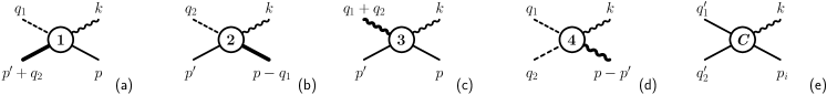
Figure 34: Contact-current diagrams with associated four-momenta. Processes with labels 1–4 in the first four diagrams correspond to contact currents labeled similarly in the two-meson production processes depicted in Fig. 22, with explicit four-momenta as in Eq. (150). The last diagram (e) depicts a generic rendering of the first four diagrams, with corresponding hadrons shown as solid lines here and generic momenta used in Eq. (161).

B.3 Four-point contact currents

The kinematics of the four contact currents labeled 1–4 in Fig. 22 for the no-loop calculation of the process

$$\gamma(k)+N(p)\to\pi_{1}(q_{1})+\pi_{2}(q_{2})+N^{\prime}(p^{\prime})$$ (150)

are indicated in Fig. 34. Their momentum dependences as used here thus are given by

$$\gamma N\to\pi B: \mathbb{C}_{1}^{\mu} =\mathbb{C}_{1}^{\mu}(p^{\prime}+q_{2},q_{1};k,p)~{},$$ (151a)

$$\gamma B\to\pi N^{\prime}: \mathbb{C}_{2}^{\mu} =\mathbb{C}_{2}^{\mu}(p^{\prime},q_{2};k,p-q_{1})~{},$$ (151b)

$$\gamma N\to\rho N^{\prime}: \mathbb{C}_{3}^{\lambda\mu} =\mathbb{C}_{3}^{\lambda\mu}(p^{\prime},q_{1}+q_{2};k,p)~{},$$ (151c)

$$\gamma\rho\to\pi\pi: \mathbb{C}_{4}^{\mu\lambda} =\mathbb{C}_{4}^{\mu\lambda}(q_{1},q_{2};k,p-p^{\prime})~{},$$ (151d)

where $B$ indicates any intermediate baryon compatible with the process. Also, $N^{\prime}$, $\pi$, and $\rho$ are placeholders for any outgoing baryon, (pseudo)scalar meson, and intermediate vector meson, respectively. The Lorentz index $\lambda$ is that of the vector meson.

It follows from the generic treatment in Appendix B.1 that the currents may be written as

$$\mathbb{C}^{\mu}_{1} =e_{1}F^{(1)}_{1}\,\hat{\Gamma}^{\mu}_{\pi}+G_{1}C^{\mu}_{1}~{},$$ (152a)

$$\mathbb{C}^{\mu}_{2} =e_{2}F^{(2)}_{2}\,\hat{\Gamma}_{\pi}+G_{2}C^{\mu}_{2}~{},$$ (152b)

$$\mathbb{C}^{\lambda\mu}_{3} =e_{\rho}F^{(\rho)}_{\rho}\,\hat{\Gamma}^{\lambda\mu}_{\rho}+G^{\lambda}_{\rho}C^{\mu}_{\rho}~{},$$ (152c)

$$\mathbb{C}^{\mu\lambda}_{4} =\big{(}e_{1}F^{(1)}_{\pi\pi}-e_{2}F^{(2)}_{\pi\pi}\big{)}\,\hat{\Gamma}^{\mu\lambda}_{\pi\pi}+G^{\lambda}_{\pi\pi}C^{\mu}_{\pi\pi}~{},$$ (152d)

where the hadronic coupling operators for the first two currents are

$$G_{k}=gG^{\pm}\frac{\not{q}_{k}}{M+m}~{},\qquad\text{for}\qquad k=1,2~{},$$ (153)

where $m$ and $M$, respectively, are the masses of the nucleon and the baryon, and $G^{\pm}$ is either $\gamma_{5}$ or $(M+m)/(M-m)$ depending on whether initial and final baryon parities are the same or not (see Ref. NOH06 for details; modifications of the present vector coupling structure by allowing scalar contributions as well are also discussed there). The couplings of the vector meson to the baryon and the meson, respectively, are given as

$$G^{\lambda}_{\rho}=-ig_{N}\left[\gamma^{\lambda}-i\kappa\frac{\sigma^{\lambda\tau}}{2m}(q_{1}+q_{2})_{\tau}\right]$$ (154)

and

$$G^{\lambda}_{\pi\pi}=-ig_{M}(q_{1}-q_{2})^{\lambda}~{}.$$ (155)

The constants $g$, $g_{N}$, and $g_{M}$ are strength parameters, and $\kappa$ is the anomalous moment of the vector meson. The form factors $F_{1}$, $F_{2}$, $F_{\rho}$, and $F_{\pi\pi}$ are phenomenological scalar functions depending on the squared four-momenta of all associated hadron legs. For the specific kinematics of Figs. 34(a)-(d), indicated by an upper index, their dependence reads

$$F^{(1)}_{1} =F_{1}\big{(}t_{1},(p’+q_{2})^{2};p^{2}\big{)}~{},$$ (156a)

$$F^{(2)}_{2} =F_{2}\big{(}q_{1}^{2},t_{2};(p-q_{1})^{2}\big{)}~{},$$ (156b)

$$F^{(\rho)}_{\rho} =F_{\rho}\big{(}t_{\rho},p^{\prime 2};p^{2}\big{)}~{},$$ (156c)

$$F^{(1)}_{\pi\pi} =F_{\pi\pi}\big{(}t_{1},q_{2}^{2};(p-p^{\prime})^{2}\big{)}~{},$$ (156d)

$$F^{(2)}_{\pi\pi} =F_{\pi\pi}\big{(}q_{1}^{2},t_{2};(p-p’)^{2}\big{)}~{},$$ (156e)

where

$$t_{1}=(q_{1}-k)^{2}~{},\quad t_{2}=(q_{2}-k)^{2}~{},\quad t_{\rho}=(q_{1}+q_{2}-k)^{2}~{}.$$ (157)

Note that

$$F_{1}(q^{2},p^{\prime 2};p^{2})=F_{2}(q^{2},p^{2};p^{\prime 2})$$ (158)

by symmetry.

Following (110), the KRt current operators are found as

$$\hat{\Gamma}^{\mu}_{\pi} =-gG^{\pm}\frac{\gamma^{\mu}}{M+m}~{},$$ (159a)

$$\hat{\Gamma}^{\lambda\mu}_{\rho} =g_{N}\frac{\sigma^{\lambda\mu}}{2m}\kappa~{},$$ (159b)

$$\hat{\Gamma}^{\mu\lambda}_{\pi\pi} =ig_{M}g^{\mu\lambda}~{},$$ (159c)

where, compared to (110), the charges have been pulled out explicitly in (152).

The final pieces for the complete description of the currents (152) are the auxiliary scalar currents corresponding to the generic results of Eq. (116). Utilizing the generic contact current depicted in Fig 34(e), they may be written as

$$C^{\mu}_{1} =C^{\mu}_{1BN}[F_{1}](q_{1},p^{\prime}+q_{2};p)~{},$$ (160a)

$$C^{\mu}_{2} =C^{\mu}_{2N^{\prime}B}[F_{2}](q_{2},p^{\prime};p-q_{1})~{},$$ (160b)

$$C^{\mu}_{\rho} =C^{\mu}_{\rho N^{\prime}N}[F_{\rho}](q_{1}+q_{2},p^{\prime};p)~{},$$ (160c)

$$C^{\mu}_{\pi\pi} =C^{\mu}_{12\rho}[F_{\pi\pi}](q_{1},q_{2};p-p^{\prime})~{},$$ (160d)

where the right-hand sides here are specific applications of the corresponding generic result. The auxiliary current for Fig 34(e) is given as

$$C^{\mu}_{12i}[h](q^{\prime}_{1},q^{\prime}_{2};p_{i}) =-e_{1}\frac{h_{1}(t_{1})-\hat{h}}{t_{1}-q^{\prime 2}_{1}}\,H^{(1)}_{2i}[\hat{h}]$$

$$\quad\mbox{}-e_{2}\frac{h_{2}(t_{2})-\hat{h}}{t_{2}-q^{\prime 2}_{2}}\,H^{(2)}_{i1}[\hat{h}]$$

$$\quad\mbox{}-e_{i}\frac{h_{i}(s_{i})-\hat{h}}{s_{i}-p^{2}_{i}}\,H^{(i)}_{12}[\hat{h}]~{},$$ (161)

written here as a functional of a generic hadronic form factor $h$, with four-momenta of incoming and outgoing hadrons labeled by $i$ and $1,2$, respectively, as in Fig. 34(e). Using Mandelstam-type squared four-momenta

$$s_{i}=(p_{i}+k)^{2}~{},\quad t_{1}=(q^{\prime}_{1}-k)^{2}~{},\quad t_{2}=(q^{\prime}_{2}-k)^{2}~{},$$ (162)

the relevant kinematic situations for the form factor read

$$h_{i}=h(q^{\prime 2}_{1},q^{\prime 2}_{2};s_{i})~{},\quad h_{1}=h(t_{1},q^{\prime 2}_{2};p_{i}^{2})~{},\quad h_{2}=h(q^{\prime 2}_{1},t_{2};p_{i}^{2})$$ (163)

and the analog of Eq. (119) for the present case is

$$H^{(1)}_{2i}[h]=\delta_{2}\frac{h_{2}}{\hat{h}}+\delta_{i}\frac{h_{i}}{\hat{h}}-\delta_{2}\delta_{i}\frac{h_{2}h_{i}}{\hat{h}^{2}}~{},$$ (164)

where $\delta_{k}=1$ if particle $k$ is charged and zero otherwise. The other functions, $H^{(2)}_{i1}[h]$ and $H^{(i)}_{12}[h]$, are obtained by cyclic permutation of indices $\{12i\}$. As usual, the expression

$$\hat{h}=h(q^{\prime 2}_{1},q^{\prime 2}_{2};p_{i}^{2})$$ (165)

provides the unphysical extrapolation to the squared external hadronic four-momenta to render Eq. (161) manifestly nonsingular, similar to Eq. (118).

Finally, note that the corresponding contact currents given in Refs. NOH06 ; MON11 differ from the ones in (152) here by manifestly transverse terms obtained by making use of the freedom of adding specific terms constructed along the lines of the generic form (125); see, in particular, remarks after Eq. (126).

References

- (1) V. Peterson and I. G. Henry, Photoproduction of mesons from hydrogen near threshold, Phys. Rev. 96, 850 (1954).
- (2) R. M. Friedman and K. M. Crowe, Photoproduction of pion pairs in hydrogen, Phys. Rev. 105, 1369 (1957).
- (3) L. J. Fretwell, Jr. and J. H. Mullins, Photoproduction of charged pion pairs from hydrogen with gamma energies up to 1500 MeV, Phys. Rev. 155, 1497 (1967).
- (4) M. G. Hauser, Photoproduction of charged pion pairs and in hydrogen from 0.9 to 1.3 GeV, Phys. Rev. 160, 1215 (1967).
- (5) R. Erbe et al. (ABBHHM Collaboration), Photoproduction of meson and baryon resonances at energies up to 5.8 GeV, Phys. Rev. 175, 1669 (1968).
- (6) R. Erbe et al. (ABBHHM Collaboration), Multipion and strange-particle photoproduction on protons at energies up to 5.8 GeV, Phys. Rev. 188, 2060 (1969).
- (7) J. Ballam et al., Bubble-chamber study of photoproduction by 2.8- and 4.7-GeV polarized photons. I. Cross-section determinations and production of and in the reaction , Phys. Rev. D 5, 545 (1972).
- (8) A. Braghieri et al., Total cross section measurement for the three double pion photoproduction channels on the proton, Phys. Lett. B 363, 46 (1995).
- (9) F. Härter, J. Ahrens, R. Beck, B. Krusche, V. Metag, M. Schmitz, H. Ströher, Th. Walcher, and M. Wolf, Two neutral pion photoproduction off the proton between threshold and 800 MeV, Phys. Lett. B 401, 229 (1997).
- (10) A. Zabrodin et al., Total cross section measurement of the reaction, Phys. Rev. C 55, R1617 (1997).
- (11) A. Zabrodin et al., Invariant mass distributions of the reaction, Phys. Rev. C 60, 055201 (1999).
- (12) V. Kleber et al., Double- photoproduction from the deuteron, Eur. Phys. J. A 9, 1 (2000).
- (13) M. Wolf et al., Photoproduction of neutral pion pairs from the proton, Eur. Phys. J. A 9, 5 (2000).
- (14) W. Langgärtner et al., Direct observation of a decay of the baryon resonance, Phys. Rev. Lett. 87, 052001 (2001).
- (15) M. Kotulla et al., Double photoproduction off the proton at threshold, Phys. Lett. B 578, 63 (2004).
- (16) Y. Assafiri et al., Double photoproduction on the proton at GRAAL, Phys. Rev. Lett. 90, 222001 (2003).
- (17) M. Ripani et al. (CLAS Collaboration), Measurement of and baryon resonance analysis, Phys. Rev. Lett. 91, 022002 (2003).
- (18) J. Ahrens et al. (GDH and A2 Collaborations), Helicity dependence of the reaction in the second resonance region, Phys. Lett. B 551, 49 (2003).
- (19) S. Strauch et al. (CLAS Collaboration), Beam-helicity asymmetries in double-charged-pion photoproduction on the proton, Phys. Rev. Lett. 95, 162003 (2005).
- (20) J. Ahrens et al. (GDH Collaboration and A2 Collaboration), Intermediate resonance excitation in the reaction, Phys. Lett. B 624, 173 (2005).
- (21) J. Ahrens et al. (GDH and A2 Collaborations), First measurement of the helicity dependence for the reaction, Eur. Phys. J. A 34, 11 (2007).
- (22) J. Ajaka et al., Double photoproduction on the neutron at GRAAL, Phys. Lett. B 651, 108 (2007).
- (23) M. Battaglieri et al. (CLAS Collaboration), Photoproduction of meson pairs on the proton, Phys. Rev. D 80, 072005 (2009).
- (24) D. Krambrich et al. (Crystal Ball at MAMI, TAPS, and A2 Collaboration), Beam-helicity asymmetries in double-pion photoproduction off the proton, Phys. Rev. Lett. 103, 052002 (2009).
- (25) G. V. Fedotov et al. (CLAS Collaboration), Electroproduction of off protons at and with the CLAS detector, Phys. Rev. C 79, 015204 (2009).
- (26) C. Wu et al. (SAPHIR Collaboration), Photoproduction of -mesons and -baryons in the reaction at energies up to GeV, Eur. Phys. J. A 23, 317 (2005).
- (27) J. Ajaka et al., Simultaneous photoproduction of and mesons on the proton, Phys. Rev. Lett. 100, 052003 (2008).
- (28) J. Junkersfeld et al. (CB-ELSA Collaboration), Photoproduction of off protons for GeV, Eur. Phys. J. A 31, 365 (2007).
- (29) M. Nanova et al. (CBELSA/TAPS Collaboration), and photoproduction off the proton, Eur. Phys. J. A 35, 333 (2008).
- (30) E. Gutz et al. (CBELSA/TAPS Collaboration), Measurement of the beam asymmetry in production off the proton with the CBELSA/TAPS experiment, Eur. Phys. J. A 35, 291 (2008).
- (31) I. Horn et al. (CB-ELSA Collaboration), Study of the reaction , Eur. Phys. J. A 38, 173 (2008).
- (32) I. Horn et al. (CB-ELSA Collaboration), Evidence for a parity doublet and from , Phys. Rev. Lett. 101, 202002 (2008).
- (33) L. Guo et al. (CLAS Collaboration), Cascade production in the reactions and , Phys. Rev. C 76, 025208 (2007).
- (34) E. Gutz et al. (CBELSA/TAPS Collaboration), Photoproduction of meson pairs: First measurement of the polarization observable , Phys. Lett. B 687, 11 (2010).
- (35) E. Gutz et al. (CBELSA/TAPS Collaboration), High statistics study of the reaction , Eur. Phys. J. A 50, 74 (2014).
- (36) V. Sokhoyan et al. (CBELSA/TAPS Collaboration), High statistics study of the reaction , Eur. Phys. J. A 51, 95 (2015), 51 187(E) (2015).
- (37) V. Sokhoyan et al. (CBELSA/TAPS Collaboration), Data on and in reveal cascade decays of via , Phys. Lett. B 746, 127 (2015).
- (38) A. Thiel et al. (CBELSA/TAPS Collaboration), Three-body nature of and resonances from sequential decay chains, Phys. Rev. Lett. 114, 091803 (2015).
- (39) E. L. Isupov et al. (CLAS Collaboration), Measurements of cross sections with CLAS at and , Phys. Rev. C 96, 025209 (2017).
- (40) E. Klempt and J.-M. Richard, Baryon spectroscopy, Rev. Mod. Phys. 82, 1095 (2010).
- (41) V. Crede and W. Roberts, Progress towards understanding baryon resonances, Rep. Prog. Phys. 76, 076301 (2013).
- (42) N. Isgur and G. Karl, Hyperfine interactions in negative parity baryons, Phys. Lett. 72B, 109 (1977).
- (43) R. Koniuk and N. Isgur, Baryon decays in a quark model with chromodynamics, Phys. Rev. D 21, 1868 (1980), 23, 818(E) (1981).
- (44) U. Thoma et al. (CB-ELSA Collaboration), and decays into , Phys. Lett. B 659, 87 (2008).
- (45) A. V. Anisovich, R. Beck, E. Klempt, V. A. Nikonov, A. V. Sarantsev, and U. Thoma, Properties of baryon resonances from a multichannel partial wave analysis, Eur. Phys. J. A 48, 15 (2012).
- (46) V. Bernard, N. Kaiser, U.-G. Meißner, and A. Schmidt, Threshold two-pion photo- and electroproduction: More neutrals than expected, Nucl. Phys. A 580, 475 (1994).
- (47) V. Bernard, N. Kaiser, and U.-G. Meißner, Comment on “Low energy expansions for double-pion photoproduction”, Phys. Rev. Lett. 74, 1036 (1995).
- (48) V. Bernard, N. Kaiser, and U.-G. Meißner, Double neutral pion photoproduction at threshold, Phys. Lett. B 382, 19 (1996).
- (49) M. Döring, E. Oset, and D. Strottman, Chiral dynamics in the and reactions, Phys. Rev. C 73, 045209 (2006).
- (50) M. Döring, E. Oset, and D. Strottman, Clues to the nature of the resonance from pion- and photon-induced reactions, Phys. Lett. B 639, 59 (2006).
- (51) M. Döring, E. Oset, and U.-G. Meißner, Evaluation of the polarization observables and in the reaction , Eur. Phys. J. A 46, 315 (2010).
- (52) H. Kamano, B. Juliá-Díaz, T.-S. H. Lee, A. Matsuyama, and T. Sato, Double and single pion photoproduction within a dynamical coupled-channels model, Phys. Rev. C 80, 065203 (2009).
- (53) A. Matsuyama, T. Sato, and T.-S. H. Lee, Dynamical coupled-channel model of meson production reactions in the nucleon resonance region, Phys. Rep. 439, 193 (2007).
- (54) H. Kamano, B. Juliá-Díaz, T.-S. H. Lee, A. Matsuyama, and T. Sato, Dynamical coupled-channels study of reactions, Phys. Rev. C 79, 025206 (2009).
- (55) J. A. Gómez Tejedor and E. Oset, A model for the reaction, Nucl. Phys. A 571, 667 (1994).
- (56) J. A. Gómez Tejedor and E. Oset, Double pion photoproduction on the nucleon: study of the isospin channels, Nucl. Phys. A 600, 413 (1996).
- (57) J. C. Nacher, E. Oset, M. J. Vicente Vacas, and L. Roca, The role of excitation and production in double pion photoproduction, Nucl. Phys. A 695, 295 (2001).
- (58) J. C. Nacher and E. Oset, Study of polarization observables in double-pion photoproduction on the proton, Nucl. Phys. A 697, 372 (2002).
- (59) L. Roca, Helicity asymmetries in double pion photoproduction on the proton, Nucl. Phys. A 748, 192 (2005).
- (60) K. Ochi, M. Hirata, and T. Takaki, Photoproduction on a nucleon in the resonance energy region, Phys. Rev. C 56, 1472 (1997).
- (61) M. Hirata, K. Ochi, and T. Takaki, Reaction mechanism in the reactions, Prog. Theor. Phys. 100, 681 (1998).
- (62) M. Hirata, N. Katagiri, and T. Takaki, coupling and two-pion photoproduction on the nucleon, Phys. Rev. C 67, 034601 (2003).
- (63) A. Fix and H. Arenhövel, Double pion photoproduction on nucleon and deuteron, Eur. Phys. J. A 25, 115 (2005).
- (64) V. I. Mokeev, M. Ripani, M. Anginolfi, M. Battaglieri, E. N. Golovach, B. S. Ishkhanov, M. V. Osipenko, G. Ricco, V. V. Sapunenko, M. Taiuti, and G. V. Fedotov, Phenomenological model for describing pion-pair production on a proton by virtual photons in the energy region of nucleon-resonance excitation, Yad. Fiz. 64, 1368 (2001), [Phys. Atom. Nucl. 64, 1292 (2001)].
- (65) V. I. Mokeev et al., Helicity components of the cross section for double charged-pion production by real photons on protons, Yad. Fiz. 66, 1322 (2003), [Phys. Atom. Nucl. 66, 1282 (2003)].
- (66) D. Jido, M. Oka, and A. Hosaka, Chiral symmetry of baryons, Prog. Theor. Phys. 106, 873 (2001).
- (67) L. Roca, E. Oset, and M. J. Vicente Vacas, The meson in a nuclear medium through two pion photoproduction, Phys. Lett. B 541, 77 (2002).
- (68) M. Hirata, K. Ochi, and T. Takaki, Cooperative damping mechanism of the resonance in the nuclear photoabsorption, Phys. Rev. Lett. 80, 5068 (1998).
- (69) Y. Oh, K. Nakayama, and T.-S. H. Lee, Pentaquark production in Reactions, Phys. Rep. 423, 49 (2006).
- (70) K. Nakayama, Y. Oh, and H. Haberzettl, Photoproduction of off nucleons, Phys. Rev. C 74, 035205 (2006).
- (71) J. K. S. Man, Y. Oh, and K. Nakayama, Role of high-spin hyperon resonances in the reaction of , Phys. Rev. C 83, 055201 (2011).
- (72) I. V. Anikin, B. Pire, L. Szymanowski, O. V. Teryaev, and S. Wallon, pair hard electroproduction and exotic hybrid mesons, Nucl. Phys. A 755, 561c (2005).
- (73) A. Kiswandhi, S. Capstick, and T.-S. H. Lee, A unitary and relativistic model for and photoproduction, Jour. Phys. Conf. Ser. 69, 012018 (2007).
- (74) V. I. Mokeev, V. D. Burkert, T.-S. H. Lee, L. Elouadrhiri, G. V. Fedotov, and B. S. Ishkhanov, Model analysis of the electroproduction reaction on the proton, Phys. Rev. C 80, 045212 (2009).
- (75) V. I. Mokeev et al. (CLAS Collaboration), Experimental study of the and resonances from the CLAS data on , Phys. Rev. C 86, 035203 (2012).
- (76) V. I. Mokeev, V. D. Burkert, D. S. Carman, L. Elouadrhiri, G. V. Fedotov, E. N. Golovatch, R. W. Gothe, K. Hicks, B. S. Ishkhanov, E. L. Isupov, and Iu. Skorodumina, New results from the studies of the , , and resonances in exclusive electroproduction with the CLAS detector, Phys. Rev. C 93, 025206 (2016).
- (77) W. Roberts and T. Oed, Polarization observables for two-pion production off the nucleon, Phys. Rev. C 71, 055201 (2005).
- (78) H. Haberzettl, Gauge-invariant theory of pion photoproduction with dressed hadrons, Phys. Rev. C 56, 2041 (1997).
- (79) H. Lehmann, K. Symanzik, and W. Zimmermann, Zur Formulierung quantisierter Feldtheorien, Nuovo Cim. 1, 205 (1955).
- (80) J. C. Ward, An identity in Quantum Electrodynamics, Phys. Rev. 78, 182 (1950).
- (81) Y. Takahashi, On the generalized Ward identity, Nuovo Cim. 6, 371 (1957).
- (82) K. Nakayama and H. Haberzettl, Interaction current in , Phys. Rev. C 80, 051001(R) (2009).
- (83) H. Haberzettl and K. Nakayama, Gauge-invariant formulation of , Phys. Rev. C 85, 064001 (2012).
- (84) H. Haberzettl, K. Nakayama, and Y. Oh, Gauge-invariant theory of two-pion photo- and electro-production off the nucleon, Few-Body Syst. 54, 1141 (2013).
- (85) L. D. Faddeev, Scattering theory for a three-particle system, Zh. Eksp. Teor. Fiz. 39, 1459 (1960), [Soviet Phys. JETP 12, 1014–1019 (1961)].
- (86) L. D. Faddeev, Mathematical Aspects of the Three-Body Problem in the Quantum Scattering Theory, Academy of Sciences of the U.S.S.R. Works of the Steklov Mathematical Institute Vol. 69 (Daniel Davey & Co., Inc., 1965).
- (87) E. O. Alt, P. Grassberger, and W. Sandhas, Reduction of the three-particle collision problem to multi-channel two-particle Lippmann-Schwinger equations, Nucl. Phys. B2, 167 (1967).
- (88) N. M. Kroll and M. A. Ruderman, A theorem on photomeson production near threshold and the suppression of pairs in pseudoscalar meson theory, Phys. Rev. 93, 233 (1954).
- (89) M. Gell-Mann and M. L. Goldberger, Scattering of low-energy photons by particles of spin 1/2, Phys. Rev. 96, 1433 (1954).
- (90) M. E. Peskin and D. V. Schroeder, An Introduction to Quantum Field Theory (Addison-Wesley, 1995).
- (91) E. Kazes, Generalized current conservation and low energy limit of photon interactions, Nuovo Cim. 13, 1226 (1959).
- (92) H. Haberzettl, C. Bennhold, T. Mart, and T. Feuster, Gauge-invariant tree-level photoproduction amplitudes with form factors, Phys. Rev. C 58, R40 (1998).
- (93) H. Haberzettl, K. Nakayama, and S. Krewald, Gauge-invariant approach to meson photoproduction including the final-state interaction, Phys. Rev. C 74, 045202 (2006).
- (94) H. Haberzettl, F. Huang, and K. Nakayama, Dressing the electromagnetic nucleon current, Phys. Rev. C 83, 065502 (2011).
- (95) H. Haberzettl, X.-Y. Wang, and J. He, Preserving local gauge invariance with -channel Regge exchange, Phys. Rev. C 92, 055503 (2015).
- (96) G. Eichmann, H. Sanchis-Alepuz, R. Williams, R. Alkofer, and C. S. Fischer, Baryons as relativistic three-quark bound states, Prog. Part. Nucl. Phys. 91, 1 (2016).
- (97) W. Sandhas, The three-body problem, Acta Phys. Austriaca Suppl. 9, 57 (1972).
- (98) F. Huang, M. Döring, H. Haberzettl, J. Haidenbauer, C. Hanhart, S. Krewald, U.-G. Meißner, and K. Nakayama, Pion photoproduction in a dynamical coupled-channels model, Phys. Rev. C 85, 054003 (2012).
- (99) K. Nakayama, Y. Oh, and H. Haberzettl, Combined analysis of meson hadro- and photo-production off nucleons, J. Korean Phys. Soc. 59, 224 (2011).
- (100) F. Huang, H. Haberzettl, and K. Nakayama, Combined analysis of production reactions: , , and , Phys. Rev. C 87, 054004 (2013).
- (101) B. C. Jackson, Y. Oh, H. Haberzettl, and K. Nakayama, reaction and hyperon resonances, Phys. Rev. C 91, 065208 (2015).
- (102) J. Landay, M. Mai, M. Döring, H. Haberzettl, and K. Nakayama, Towards the minimal spectrum of excited baryons, arXiv:1810.00075.
- (103) P. Grassberger and W. Sandhas, Systematical treatment of the non-relativistic -particle scattering problem, Nucl. Phys. B2, 181 (1967).
- (104) W. Sandhas, The -body problem, Acta Phys. Austriaca Suppl. 13, 679 (1974).
- (105) W. Sandhas, -body integral equations and four-nucleon calculations, Czech. J. Phys. B25, 251 (1975).
- (106) E. O. Alt, P. Grassberger, and W. Sandhas, Treatment of the three- and four-nucleon systems by a generalized separable-potential model, Phys. Rev. C 1, 85 (1970).
- (107) S. D. Drell and T. D. Lee, Scaling properties and the bound-state nature of the physical nucleon, Phys. Rev. D 5, 1738 (1972).