Practical Batch Bayesian Optimization for Less Expensive Functions

Abstract

Bayesian optimization (BO) and its batch extensions are successful for optimizing expensive black-box functions. However, these traditional BO approaches are not yet ideal for optimizing less expensive functions when the computational cost of BO can dominate the cost of evaluating the black-box function. Examples of these less expensive functions are cheap machine learning models, inexpensive physical experiment through simulators, and acquisition function optimization in Bayesian optimization. In this paper, we consider a batch BO setting for situations where function evaluations are less expensive. Our model is based on a new exploration strategy using geometric distance that provides an alternative way for exploration, selecting a point far from the observed locations. Using that intuition, we propose to use Sobol sequence to guide exploration that will get rid of running multiple global optimization steps as used in previous works. Based on the proposed distance exploration, we present an efficient batch BO approach. We demonstrate that our approach outperforms other baselines and global optimization methods when the function evaluations are less expensive.

1 Introduction

Bayesian optimization (BO) has received considerable attention in tuning hyper-parameters for complex models and algorithms Brochu et al. (2010); Hennig and Schuler (2012); Snoek et al. (2012); Shahriari et al. (2016). In a standard setting, BO suggests one evaluation at a time, whereas batch BO can recommend multiple evaluations where parallel facilities are available. The batch setting is essential to speed up the optimization. Such scenarios appear, for instance, in optimizing computer models where several cores are available for parallel runs. Another example is in wet-lab experiments, wherein the need for batch experiments is significant as the cost of testing one experiment is the same as testing a batch.

Typically, batch Bayesian optimization considers addressing the expensive black-box functions in which the computational cost of batch approaches are negligible with respect to the function evaluation cost. In such cases, the computation of batch algorithms may not influence the optimization performance. On the contrary, if the function evaluation is cheap, one can make use of the global optimization techniques, such as Direct or multi-start Newton method. Thus, a computationally expensive batch BO approach may not be the right choice when the function evaluation is cheap.

However, there are many less expensive optimization problems where function evaluations (including evaluating time and economic cost) are neither highly expensive nor so cheap. When optimizing these functions, the computation of batch BO becomes sensitive and plays an important role in the optimization performance. To highlight such computational effects, in the experiments, we specifically consider the less expensive functions including machine learning models training on medium size datasets, inexpensive physical experiment via simulators, and acquisition function optimization (an auxiliary step in BO). The existing batch Bayesian optimization techniques may not be well suited for these functions. This is because their computations can be slower than the black-box function evaluations and thus the cheap global optimization techniques are more favorable.

In this paper, we consider batch Bayesian optimization problem for situations where the black-box function evaluation is less expensive in terms of evaluation time and economic cost. To make batch algorithm efficient, we design to select a first point in the batch using a standard BO and the remaining points in cheaper computational ways. For this purpose, we propose a new data-driven space filling strategy, called distance exploration (DE). Our intuition for distance exploration is based on the fact that the best location for exploration should not be close to the existing observations. We propose to use Sobol sequence Sobol’ (1967) to find such explorative points efficiently. Despite of being simple, our strategy maintains the desirable property of exploration. In addition, our model enjoys computational advantage as our model only needs to perform a single global optimization step, as opposed to all other existing batch Bayesian optimization approaches which either sequentially perform $B$ global optimizations Desautels et al. (2014); Kathuria et al. (2016); Contal et al. (2013) (where $B$ is a batch size) or solves even more complex approximation Shah and Ghahramani (2015); Wu and Frazier (2016); Daxberger and Low (2017). We validate our model using an extensive set of benchmark functions and selected real-world applications which are less expensive. These experiments demonstrate that our distance exploration (DE) approach outperforms all the baselines in terms of computation while being competitive in finding the optimal value. Our main contributions are

• A first study of Bayesian optimization to tackle the problem of less expensive function evaluation.

• A novel view for exploration using distance and a batch BO approach using distance exploration.

• Validation on benchmark and real applications where evaluations are not highly expensive.

2 Batch BO for Less Expensive Functions

To address the problem of less expensive black-box function, we aim to propose a scalable batch BO algorithm whose computation is faster than such black-boxes. Before going to detail of the proposed method, we briefly summarize and motivate from the existing approaches.

Most of the existing work in batch Bayesian optimization Contal et al. (2013); Desautels et al. (2014); González et al. (2016) try to find locations based on the shape of the posterior and the values that one might observe at the next point being sampled. However, BO may not reach to its asymptotic convergence because the accurate GP posteriors can never be obtained due to (1) given limited observations and (2) the imperfection of the GP hyper-parameter estimation, as mentioned in Wang and de Freitas (2014).

One way to improve Bayesian optimization is through the GP surrogate model. To improve the GP surrogate model of the black-box function $f$, it is intuitive to gain information about $f$ as much as possible. By gaining more information about $f$, we can have a better fitting of a GP surrogate. This can be done by picking the first point in the batch to be the optimum of our standard BO, i.e., via UCB Srinivas et al. (2010) or EI Mockus_1978Application acquisition function, and choosing the remaining points in the batch by using a cheaper strategy. Such a cheaper strategy will help us to address the less expensive function setting.

2.1 The Proposed UCB-DE

To make a batch BO algorithm efficient, we propose to select the first element in the batch as the standard BO $\mathbf{x}_{t,1}=\arg\max_{\mathbf{x}\in\mathcal{X}}\thinspace\alpha_{t}^{\textrm{UCB}}\left(\mathbf{x}\right)$. Here, we use the GP-UCB Srinivas et al. (2010) which possesses the nice convergent analysis although this can be applicable for other acquisition functions. After obtaining the first element by UCB, we fill in a space with a batch of $B-1$ points $\mathbf{x}_{t,b},\forall b\in\{2,...,B\}$ by using distance exploration (DE) presented in the next section. This step aims to gather a batch of diversity points to gain information about the black-box function $f$ in a cheap computation way. We summarize our UCB-DE in Algorithm 1.

Algorithm 1 UCB-DE for Batch Bayesian Optimization.

   Input: initial data $\mathcal{D}_{0}$, #iter $T$, batch size $B$, $l(\mathbf{a},\mathbf{b})=\sum_{j=1}^{d}\frac{1}{\sigma_{j}}||a_{j}-b_{j}||^{2}$, $g(\mathbf{x},\mathcal{D})=\min_{\mathbf{x}_{i}\in\mathcal{D}}l(\mathbf{x},\mathbf{x}_{i})$

1:   Generate $S=\left[\mathbf{s}_{1}...\mathbf{s}_{M}\right]\sim\textrm{Sobol}$ sequence

2:  for  $t=1$ to $T$  do

3:      Obtain $\mathbf{x}_{t,1}=\arg\max_{\mathbf{x}\in\mathcal{X}}\thinspace\alpha_{t}^{\textrm{UCB}}\left(\mathbf{x}\right)$

4:      Augment $\mathcal{D}_{t,1}=\mathcal{D}_{t-1}\cup\mathbf{x}_{t,1}$

5:     for  $i=2$ to $B$  do

6:         Select $\mathbf{x}_{t,i}=\arg\max_{\forall\mathbf{s}\in S}g\left(\mathbf{s},\mathcal{D}_{t,i-1}\right)$

7:         Augment $\mathcal{D}_{t,i}=\mathcal{D}_{t,i-1}\cup\mathbf{x}_{t,i}$

8:     end for

9:      Evaluate in parallel $y_{t,b}=f\left(\mathbf{x}_{t,b}\right),\forall b\leq B$

10:      Augment $\mathcal{D}_{t}=\mathcal{D}_{t-1}\cup\left(\mathbf{x}_{t,b},y_{t,b}\right)_{b=1}^{B}$

11:  end for

   Output: a recommendation $\mathbf{x}^{*}=\arg\max_{\mathbf{x}\in\mathcal{X}}\mu(\mathbf{x}\mid\mathcal{D}_{T})$

Our approach spends $B-1$ points in a batch to gain information about the black-box function $f$. We guide it to select the points which are as far as possible from the existing observations to learn about $f$. This way will help to estimate better the GP model (a surrogate model of $f$) which later informs to select a next point. Since the first point in a batch is using a standard BO, our model still performs exploitation to find the optimum, one of the key factor in decision making. In other words, our approach uses $B-1$ points for exploration and a point for exploitation in each iteration.

Our approach requires only one run of global optimization, opposed to all other existing batch BO approaches which either sequentially perform $B$ global optimizations Desautels et al. (2014); Kathuria et al. (2016); Contal et al. (2013) or solve even more complex approximation Shah and Ghahramani (2015); Wu and Frazier (2016); Nguyen et al. (2016b); Daxberger and Low (2017); Wang et al. (2018).

2.2 Distance Exploration (DE)

We present a simple, but effective, strategy for filling the $B-1$ remaining points in a batch, called distance exploration. We first summarize that the traditional space filling strategies can not take into account the existing observations to make the best space-filling. Then, we describe the proposed distance exploration and discuss some useful properties.

2.2.1 Data-driven space filling strategies.

There are existing well known strategies for space filling, such as Latin hypercube design McKay et al. (1979) and Sobol sequence Sobol’ (1967). However, most of such strategies are not designed for data-driven setting, or under the presence of observations. Example of the Sobol sequence is in Fig. 1. We can see that the points in the vanilla Sobol sequence are not yet optimal for exploration as they may locate near the existing observations. This is because the vanilla Sobol sequence is unable to take into account the existing observations to make a better design. In our setting of batch BO, we aim to fill a space such that we do not want to assign points close to the existing observations. The conventional space filling approaches Sobol’ (1967) are restricted for this scenario, to our knowledge.

2.2.2 Distance exploration (DE) for data-driven space filling.

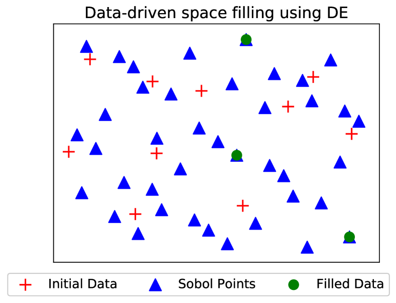
Figure 1: Examples of DE to fill a space with $3$ extra points given $10$ initial observed locations ($+$) . We first use a Sobol sequence $\Delta$ of $40$ points to approximately find the good location which is far from the existing observations. Then, we pick the best point from this Sobol sequence and add this point into the observation set. We repeat the process until a batch is filled. This process is done without requiring a global optimization.

We propose a space filling approach given the existence of the observed locations. Intuitively, we aim to fill in a space with high uncertainty points which should not be close to already observed locations. If a considered data point stays closer to an observed location, the less uncertainty it gets, and vice versa. Thus, we can employ the distance from an arbitrary location to the observed locations as a guide for filling a space. That is, we sequentially fill a space with the location $\mathbf{x}_{t}$ s.t. the distance from $\mathbf{x}_{t}$ to its nearest observation $\mathbf{x}_{i}\in\mathcal{D}_{t}$ is maximized, i.e. $\mathbf{x}_{t}=\arg\max_{\mathbf{x}\in\mathcal{X}}\thinspace||\mathbf{x}-[\mathbf{x}]||^{2}$ where we denote a nearest observation to $\mathbf{x}$ as $[\mathbf{x}]=\arg\min_{\mathbf{x}_{i}\in\mathcal{D}_{t}}||\mathbf{x}-\mathbf{x}_{i}||^{2}$ and $\mathcal{D}_{t}$ is the observation set at iteration $t$. By using distance for data-driven space filling, our DE offers the alternative exploration to a Gaussian process predictive variance while DE gets rid of cubic operation of these methods. Formally, we seek for the point which is far from the existing observations, i.e.,

$$\mathbf{x}_{t} =\underset{{}_{\mathbf{x}\in\mathcal{X}}}{\text{argmax}}\thinspace[\underset{{}_{\mathbf{x}_{i}\in\mathcal{D}_{t}}}{\text{argmin}\ }l(\mathbf{x},\mathbf{x}_{i})].$$ (1)

where the $\arg\min$ is computed from a finite set of $\mathcal{D}_{t}$ and $\arg\max$ can be computed using either a global optimization on a continuous domain $\mathcal{X}$ or a Sobol approximation in the below section.

2.3 Finding The Farthest Points Efficiently

One can optimize the Eq. (1) directly to find the farthest point, $\mathbf{x}\in\mathcal{X}$, from the existing observation set $\mathcal{D}_{t}$ by running a global optimization. However, running $B-1$ global optimizations will be expensive, especially for high dimensional functions, and finding the exact locations may not be necessary since we will not directly use such points for final recommendation. Instead, these points are used to gain information for estimating a better GP surrogate model.

Therefore, we propose an efficient algorithm to find the farthest points without using global optimization. Our idea is as the following. Initially, we generate a Sobol sequence Sobol’ (1967) including $M$ points, $S=[\mathbf{s}_{1},...,\mathbf{s}_{M}],\mathbf{s}_{m}\in\mathcal{R}^{d}$. This step is required to compute once in advance. Then, at each iteration $t$, we evaluate the “explorative score” at those Sobol points using a function $\min_{\mathbf{x}_{i}\in\mathcal{D}_{t}}l(\mathbf{s}_{m},\mathbf{x}_{i})$. Based on such scores, we can approximately compute the Eq. (1) to choose the farthest point as

$$\mathbf{x}_{t} =\underset{{}_{\forall\mathbf{s}_{m}\in S}}{\text{argmax}}[\underset{{}_{\mathbf{x}_{i}\in\mathcal{D}_{t}}}{\text{argmin}\ }l(\mathbf{x},\mathbf{x}_{i})].$$ (2)

Next, we add this found point into the observation set (in a greedy manner) $D_{t,i}=D_{t,i-1}\cup\mathbf{x}_{t}$ and sequentially repeat this process to fill a remaining $B-1$ points in a batch while the first point in a batch will be chosen by the standard GP-UCB.

An example of distance exploration for space filling is illustrated in Fig. 1. Given the $10$ initial observed locations ($+$) $\mathcal{D}_{t}$, we generate $40$ Sobol sequences ($\Delta$) then we fill a space with $3$ additional points by choosing the best points from the Sobol sequence.

2.4 Computational Complexity

Let $T$ denote #iteration, $B$ #batch size, $d$ #dimension, $N=TB$ #observation. In BO, global optimization, which repeatedly evaluates the acquisition function, is used to select a point. Let the number of evaluations in global optimization be $C_{d}$ as a function of the dimension $d$. Both BUCB Desautels et al. (2014) and our approach are similar in computing the first point in a batch with the complexity of $\mathcal{O}(C_{d}TN^{2})$ where the Cholesky decomposition is used for matrix inversion.

The difference in computation is from selecting $B-1$ points. In BUCB, , the total cost for selecting $B-1$ elements in $T$ iteration is $\mathcal{O}\left[T(B-1)(N^{2}+C_{d}N^{2})\right]$. By noting that $N=TB$, we have $\mathcal{O}(C_{d}N^{3})$ and thus the total complexity of BUCB (also applicable for CL, UCB-PE and DPP) is $\mathcal{O}(C_{d}\left[TN^{2}+N^{3}\right])$.

In our UCB-DE, the computation of Sobol sequence is pre-computed once. The cost for finding a nearest point in $\mathcal{D}_{t}$ is also cheap $\mathcal{O}(N)$. Thus, our UCB-DE is $\mathcal{O}(C_{d}TN^{2})$, much cheaper than BUCB.

2.5 Evaluation of Performance

In our setting, the points selected by the distance exploration are different from the posterior maximum and does not represent the best guess for the global minimizer at each step. On the other hand, when using the batch strategy based on the values observed, such as GP-BUCB Desautels et al. (2014) and LP González et al. (2016), these points do still provide good results. However, when using distance exploration, the chosen points do not necessary contain high function values. We therefore propose a greedy evaluation at the posterior minimum as the final step of optimization. That is, after $t$ iterations, we take the recommendation point as $\tilde{\mathbf{x}}_{t}=\arg\max_{\mathbf{x}\in\mathcal{X}}\mu(\mathbf{x}\mid\mathcal{D}_{t})$ and use $f(\tilde{\mathbf{x}}_{t})$ for comparison. This strategy is also popularly used for evaluating information-theoretic BO approaches Hennig and Schuler (2012); Hernández-Lobato et al. (2014); Ru et al. (2018).

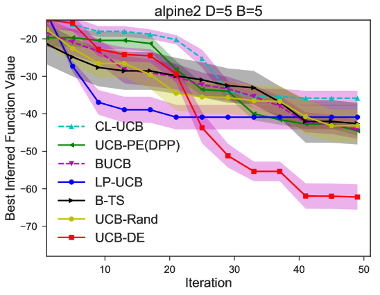
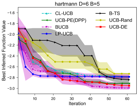
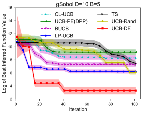
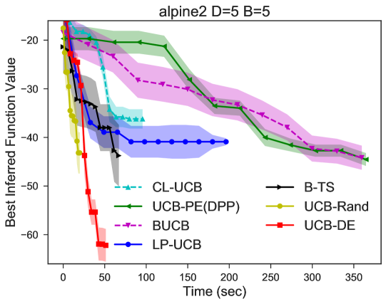
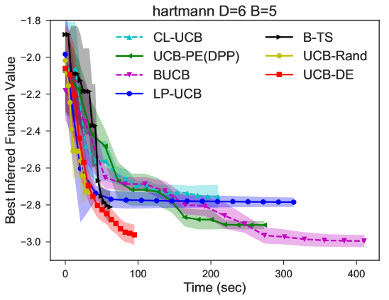
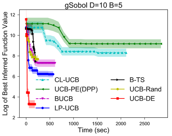
Figure 2: Top: comparison on iteration axis. Bottom: comparison on time axis which is suitable for a setting of less expensive function. Our approach achieves superior performance within limited time. Best viewed in color.

3 Experiments

We first demonstrate the efficiency of our UCB-DE against the baselines on benchmark functions. Next, we highlight our model on optimizing the less expensive functions. Finally, we analyze the computational complexity.

Experimental setting.

Given dimension $d$, the optimization is run with an evaluation budget of $T=10d$ and the initial $3d$ points. The input is scaled $\mathbf{x}\sim\left[0,1\right]^{d}$ and the output is standardized $y\sim\mathcal{N}\left(0,1\right)$ for robustness. Although our DE is applicable for anisotropic case of the distance, we use the isotropic Euclidean distance for simplicity since our main goal is to demonstrate the scalability for optimizing less expensive function. For other BO approaches, we use the isotropic squared exponential (SE) kernel $k\left(\mathbf{x},\mathbf{x^{\prime}}\right)=\exp\left(-l(\mathbf{x},\mathbf{x^{\prime}})|^{2}\right)$ where $l(\mathbf{a},\mathbf{b})=\frac{1}{\sigma_{l}}||\mathbf{a}-\mathbf{b}||^{2}$ and $\sigma_{l}$ is chosen by maximizing the GP marginal likelihood Rasmussen (2006). We repeat the experiments $20$ times and report the mean and standard error. All implementations are in Python on a Windows machine Core i7 Ram 24GB. For the experimental evaluation, after $t$ iterations, we take the recommendation point as the maximum of the GP posterior, i.e., $\tilde{\mathbf{x}}_{t}=\arg\max_{\mathbf{x}\in\mathcal{X}}\mu(\mathbf{x}\mid\mathcal{D}_{t})$ and use $f(\tilde{\mathbf{x}}_{t})$ for comparison. We note that other batch approaches, such as BUCB, using either $f(\tilde{\mathbf{x}}_{t})$ or $\max_{\forall i\leq t}f(\mathbf{x}_{t})$ will result in similar performance. We use a Sobol sequence with $M=10\times T\times B$ points.

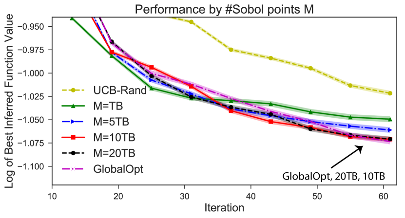
Figure 3: Comparison with different choices of $M$. Our approach UCB-DE using Sobol sequence $M\geq 10TB$ achieves comparable performance to using continuous global optimization.

Baselines.

We use common batch BO baselines and global optimization methods for comparison. These baselines include Constant liar (CL) Ginsbourger et al. (2010) and local penalization (LP) González et al. (2016) from GPyOpt toolbox. GP-BUCB Desautels et al. (2014), UCB pure exploration (PE) Contal et al. (2013) and determinantal point process (DPP) Kathuria et al. (2016). The UCB-PE is shown as equivalent to the greedy DPP. Thus, in the experiment, we denote UCB-PE (DPP) for comparing these two baselines. UCB-Rand: select a first point in a batch by GP-UCB and the remaining points by random. Batch Thompson sampling (B-TS): although the batch TS approach Hernández-Lobato et al. (2017); Kirthevasan et al. (2018) is presented for distributed setting, we restrict B-TS non-distributed in this paper. Random search, L-BFGS-B (with multi-start) in Scipy and Direct in nlopt package Johnson (2014).

3.1 Model analysis on number of Sobol points $M$

We analyze our model performance by varying the number of Sobol points in Fig. 3. Using Hartmann $d=6$ function, we can see that increasing $M$ can likely improve the performance which is converged after $M\geq 10TB$. Although we fix the number of samples $M=10TB$ in the experiments, we would suggest increasing this value if we have generous computational budget.

In addition, we empirically show that our approach using Sobol sequence in Eq. (2) with sufficiently number of points $M$ (e.g., $10TB$ or $20TB$) achieves comparable performance to the case of using continuous global optimization, as in Eq. (1). The first reason is by the imperfectness of the global optimization. The second reason is that we may not need to find the exact farthest points for the purpose of exploration.

The UCB-Rand is inferior to UCB-DE irrespective of the choices $M$. This is because of the property of Sobol sequence Sobol’ (1967) makes the points diversed while there is no such guarantee for random points.

3.2 Comparison on benchmark functions

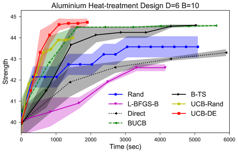
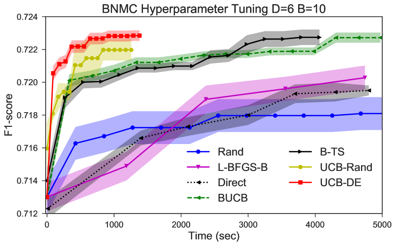
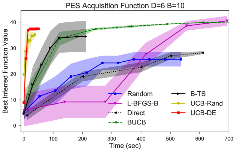
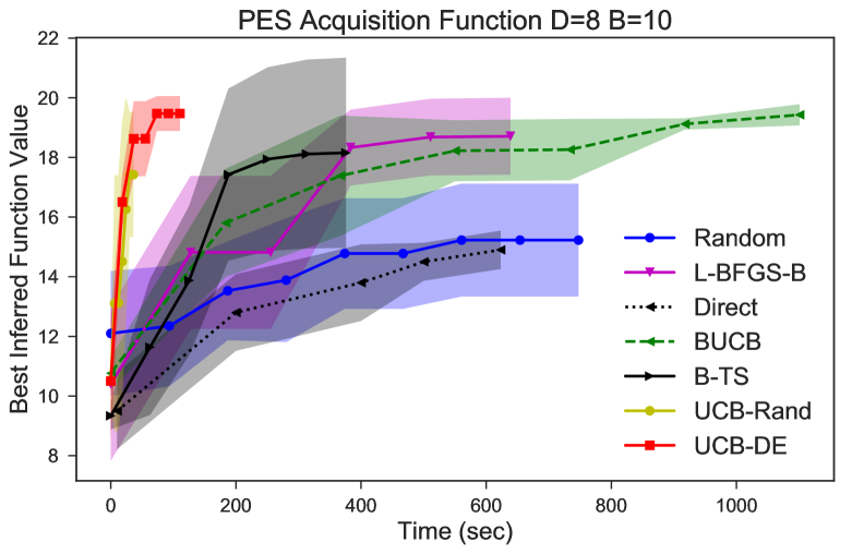
Figure 4: Optimizing less expensive black-box functions in a time axis (including the time for BO and for evaluating experiments in parallel). UCB-DE outperforms the baselines within the shortest time. When function evaluations are a bit more expensive (top row), the BO approaches are clearly better than the global optimization.

We compare our UCB-DE with batch BO baselines on benchmark functions in Fig. 2 under the iteration axis (top) and time axis (bottom). All of the BO methods perform generally well and competitive because they are similar in selecting the first element in a batch (except B-TS). The key difference is from selecting the remaining $B-1$ points. Our proposed UCB-DE performs better than the baselines. This is because DE selects points far away from the existing observations to learn better the GP surrogate model. We improve the optimization by improving our surrogate model. In addition, selecting points by distance exploration is beneficial against the GP predictive variance in such a way that GP variance is crucially sensitive to the choice of kernel length-scale parameter which may not be estimated accurately given limited observations. As a result, our UCB-DE gains favorable performance against the baselines. In particular, for alpine2 and gSobol functions which require more exploration, our UCB-DE significantly outperforms all competitors by a wide margin.

Another useful property of our UCB-DE is the computational advantage. Using a time axis (Fig. 2 bottom), we highlight that our UCB-DE outperforms the others within a short period. UCB-DE is better than UCB-Rand because the DE can gather information optimally than random which can select points near the existing observations.

3.3 Batch BO for less expensive experiments

We demonstrate the effectiveness of our UCB-DE on real-world applications where the function evaluations are less expensive. Specifically, we pick the experiments such that each experiment evaluation is in a range of $1-10$ times the CPU computation of the batch BO algorithm. We select three experiments with the decreasing expensiveness order as (1) physical heat-treatment design, (2) machine learning model, and (3) optimizing the PES acquisition functions. We use a batch size $B=10$ and the number of iteration is $T=10d$ for the batch approaches whereas the global optimization solvers can take more evaluations given the same time budget.

Heat-treatment design for Aluminum.

We consider the alloy hardening process of Aluminum-scandium Kampmann and Wagner (1983) consisting of three stages each of which includes a choice of time and temperature. We aim to maximize the strength for alloys by designing the appropriate times and temperatures. Thus, we have 6 experimental design choices to tune. We collaborate with the metallurgists to evaluate the strength using the KWN Matlab simulator. Each evaluation takes about $30$ secs.

Tuning cheap machine learning model.

We optimize the hyper-parameters for the multi-label classification algorithm of BNMC Nguyen et al. (2016a) on Scene dataset using the available code. There are 6 hyper-parameters to tune so that the F1-score is maximized. Each evaluation takes $20$ secs.

PES acquisition function.

Optimizing the acquisition function to select a next evaluation is a common strategy in BO. Gradient-based optimizer is ideal for this step when the acquisition function has the derivative information available (e.g., EI and UCB). However, it is not the case for information theoretic acquisition functions, such as Predictive entropy search Hernández-Lobato et al. (2014) because of multiple assumptions and approximation by expectation propagation which does not guarantee to converge and often leads to numerical instabilities. Formally, we consider $\alpha^{\textrm{PES}}$ a less expensive black-box function and use batch BO to optimize $\mathbf{x}_{t}=\arg\max\alpha^{\textrm{PES}}(\mathbf{x})$. Each evaluation of $\alpha^{\textrm{PES}}(\mathbf{x})$ takes $2$ secs although finding $\arg\max\alpha^{\textrm{PES}}(\mathbf{x})$, requiring many evaluations, will take $800-3000$ secs.

Analyzing the results.

We report the results in Fig. 4. It can be seen that the performance of B-TS and Random approaches are in high uncertainty than the others. Although the Random, L-BFGS-B (with multi-start) and Direct can take more evaluations, they generally perform worse than the BO approaches. This is because BO approaches, with theoretical guarantee, can balance exploration and exploitation to reach to the better location using less evaluations.

When function evaluations are a bit more expensive (i.e. heat-treatment and BNMC in the Top Fig. 4), the BO approaches are clearly better than all global optimization approaches. On the other hand, for cheaper evaluation functions of PES, the L-BFGS-B (with multi-start) will perform well (see Bottom Fig. 4).

The experiments show that our UCB-DE overall achieves the best performance within the shortest time (see Fig. 4). Although BUCB also gains good optimization values (similar to ours) at the end, it takes BUCB $3-6$ times slower than our UCB-DE to reach there. We remark that a random search (Random in Fig. 4) results in poor performance especially in high dimension whereas a random search with UCB (or UCB-Rand) performs surprisingly well. Specifically, we demonstrate that using our UCB-DE can speed up the optimization cost for PES acquisition function Hernández-Lobato et al. (2014) from $800$ secs in $d=6$ to $100$ secs for the same optimal value.

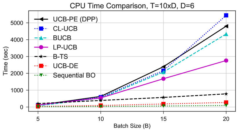
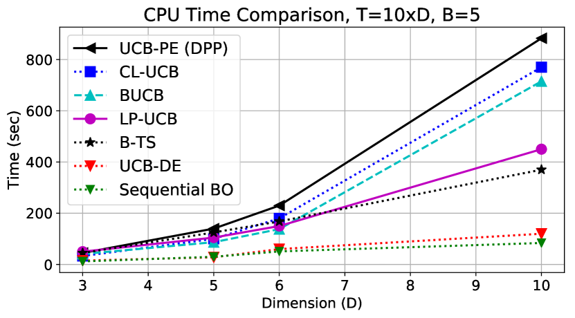
Figure 5: Time comparison with different batch size $B$ and dimensions $d$. The proposed UCB-DE is the fastest batch BO method.

3.4 Computation complexity comparison

In Fig. 5, we study the computational time w.r.t. different batch sizes $B=5,10,15,20$ on Hartmann 6D function and different dimensions $d=3,5,6,10$.

We learn from Fig. 5 that UCB-PE (DPP) takes more computation than the others because it repeatedly computes relevant regions and searches for the highest variance location in these regions. BUCB only updates the predictive variance while it keeps the mean function fixed. Hence, BUCB is cheaper than CL which requires updating both mean and variance. Local penalization (LP) González et al. (2016) is faster than BUCB. This is because LP does not recompute GP after adding each element in a batch, instead LP maintains a penalized cost after inserting each element.

Our proposed approach significantly runs faster than the others. Especially, when a batch size $B$ increases, our UCB-DE computation seems invariant and surpasses the others in an order of magnitude. Because increasing a batch size results in more observations and requires to perform more global optimization steps, the complexity of BUCB is increased while our UCB-DE is much cheaper.

4 Conclusion

In this paper, we have considered a novel setting in optimizing the less expensive black-box functions. To address this less expensive setting, we have presented an algorithm UCB-DE for batch Bayesian optimization. While our approach is simple to implement, it maintains desirable properties of exploration. Our proposed DE greatly speeds up the computation for batch BO that we do not need to run multiple global optimization to fill a batch. We demonstrate that the proposed UCB-DE is the best batch BO approach for optimizing the less expensive black-box functions.

References

- Brochu et al. [2010] Eric Brochu, Vlad M Cora, and Nando De Freitas. A tutorial on bayesian optimization of expensive cost functions, with application to active user modeling and hierarchical reinforcement learning. arXiv preprint arXiv:1012.2599, 2010.
- Contal et al. [2013] Emile Contal, David Buffoni, Alexandre Robicquet, and Nicolas Vayatis. Parallel gaussian process optimization with upper confidence bound and pure exploration. In Machine Learning and Knowledge Discovery in Databases, pages 225–240. Springer, 2013.
- Daxberger and Low [2017] Erik A Daxberger and Bryan Kian Hsiang Low. Distributed batch gaussian process optimization. In International Conference on Machine Learning, pages 951–960, 2017.
- Desautels et al. [2014] Thomas Desautels, Andreas Krause, and Joel W Burdick. Parallelizing exploration-exploitation tradeoffs in gaussian process bandit optimization. The Journal of Machine Learning Research, 15(1):3873–3923, 2014.
- Ginsbourger et al. [2010] David Ginsbourger, Rodolphe Le Riche, and Laurent Carraro. Kriging is well-suited to parallelize optimization. In Computational Intelligence in Expensive Optimization Problems, pages 131–162. Springer, 2010.
- González et al. [2016] Javier González, Zhenwen Dai, Philipp Hennig, and Neil D Lawrence. Batch Bayesian optimization via local penalization. In International Conference on Artificial Intelligence and Statistics, pages 648–657, 2016.
- Hennig and Schuler [2012] Philipp Hennig and Christian J Schuler. Entropy search for information-efficient global optimization. Journal of Machine Learning Research, 13:1809–1837, 2012.
- Hernández-Lobato et al. [2014] José Miguel Hernández-Lobato, Matthew W Hoffman, and Zoubin Ghahramani. Predictive entropy search for efficient global optimization of black-box functions. In Advances in Neural Information Processing Systems, pages 918–926, 2014.
- Hernández-Lobato et al. [2017] José Miguel Hernández-Lobato, James Requeima, Edward O Pyzer-Knapp, and Alán Aspuru-Guzik. Parallel and distributed thompson sampling for large-scale accelerated exploration of chemical space. In International Conference on Machine Learning, pages 1470–1479, 2017.
- Johnson [2014] Steven G Johnson. The nlopt nonlinear-optimization package, 2014.
- Kampmann and Wagner [1983] R Kampmann and R Wagner. Kinetics of precipitation in metastable binary alloys-theory and applications to cu-1.9 at% ti and ni-14 at% al. In Decomposition of Alloys: The Early Stages, Proceedings of the 2 nd Acta-Scripta Metallurgica Conference, pages 91–103, 1983.
- Kathuria et al. [2016] Tarun Kathuria, Amit Deshpande, and Pushmeet Kohli. Batched gaussian process bandit optimization via determinantal point processes. In Advances in Neural Information Processing Systems, pages 4206–4214, 2016.
- Kirthevasan et al. [2018] Kandasamy Kirthevasan, Krishnamurthy Akshay, Schneider Jeff, and Poczos Barnabas. Parallelised bayesian optimisation via thompson sampling. In AISTATS, 2018.
- McKay et al. [1979] Michael D McKay, Richard J Beckman, and William J Conover. Comparison of three methods for selecting values of input variables in the analysis of output from a computer code. Technometrics, 21(2):239–245, 1979.
- Nguyen et al. [2016a] Vu Nguyen, Sunil Gupta, Santu Rana, Cheng Li, and Svetha Venkatesh. A Bayesian nonparametric approach for multi-label classification. In Proceedings of The 8th Asian Conference on Machine Learning (ACML), pages 254–269, 2016.
- Nguyen et al. [2016b] Vu Nguyen, Santu Rana, Sunil K Gupta, Cheng Li, and Svetha Venkatesh. Budgeted batch Bayesian optimization. In 16th International Conference on Data Mining (ICDM), pages 1107–1112, 2016.
- Rasmussen [2006] Carl Edward Rasmussen. Gaussian processes for machine learning. 2006.
- Ru et al. [2018] Binxin Ru, Michael Osborne, and Mark McLeod. Fast information-theoretic bayesian optimisation. In International Conference on Machine Learning, 2018.
- Shah and Ghahramani [2015] Amar Shah and Zoubin Ghahramani. Parallel predictive entropy search for batch global optimization of expensive objective functions. In Advances in Neural Information Processing Systems, pages 3312–3320, 2015.
- Shahriari et al. [2016] Bobak Shahriari, Kevin Swersky, Ziyu Wang, Ryan P Adams, and Nando de Freitas. Taking the human out of the loop: A review of Bayesian optimization. Proceedings of the IEEE, 104(1):148–175, 2016.
- Snoek et al. [2012] Jasper Snoek, Hugo Larochelle, and Ryan P Adams. Practical Bayesian optimization of machine learning algorithms. In Advances in neural information processing systems, pages 2951–2959, 2012.
- Sobol’ [1967] Il’ya Meerovich Sobol’. On the distribution of points in a cube and the approximate evaluation of integrals. Zhurnal Vychislitel’noi Matematiki i Matematicheskoi Fiziki, 7(4):784–802, 1967.
- Srinivas et al. [2010] Niranjan Srinivas, Andreas Krause, Sham Kakade, and Matthias Seeger. Gaussian process optimization in the bandit setting: No regret and experimental design. In Proceedings of the 27th International Conference on Machine Learning, pages 1015–1022, 2010.
- Wang and de Freitas [2014] Ziyu Wang and Nando de Freitas. Theoretical analysis of bayesian optimisation with unknown gaussian process hyper-parameters. arXiv preprint arXiv:1406.7758, 2014.
- Wang et al. [2018] Zi Wang, Clement Gehring, Pushmeet Kohli, and Stefanie Jegelka. Batched large-scale bayesian optimization in high-dimensional spaces. In International Conference on Artificial Intelligence and Statistics, pages 745–754, 2018.
- Wu and Frazier [2016] Jian Wu and Peter Frazier. The parallel knowledge gradient method for batch Bayesian optimization. In Advances In Neural Information Processing Systems, pages 3126–3134, 2016.