Current cross-correlation in the Anderson impurity model with exchange interaction

Abstract

We study spin-entanglement of the quasiparticles of the local Fermi liquid excited in nonlinear current through a quantum dot described by the Anderson impurity model with two degenerate orbitals coupled to each other via an exchange interaction. Applying the renormalized perturbation theory, we obtain the precise form of the cumulant generating function and cross-correlations for the currents with spin angled to arbitrary directions, up to third order in the applied bias voltage. It is found that the exchange interaction gives rise to spin-angle dependency in the cross-correlation between the currents through the two different orbitals, and also brings an intrinsic cross-correlation of currents with three different angular momenta.

I Introduction

In dilute magnetic alloys, a magnetic moment in an impurity and that of surrounding conduction electrons in the host metal form a singlet ground state at low temperatures. This phenomenon, known as the Kondo effect, has been intensively studied as a central issue of the condensed matter physics from the impurity problem to the heavy Fermions since the discovery of the mechanism. Hewson (1993a) Recently, development in modern condensed matter systems such as semiconductor quantum dots, ultracold atoms, and condensed quarks, has stimulated further research to explore new aspects of the Kondo effect. Goldhaber-Gordon et al. (1998); van der Wiel et al. (2000); Buccheri et al. (2016); Hattori et al. (2015); Ozaki et al. (2016) In quantum dots, the Kondo effect in the nonequilibrium steady state beyond the linear response regime has been achieved by applying small bias-voltages, which has been shedding light on a new aspect of the local Fermi liquid. Oguri (2001); Grobis et al. (2008); Kretinin et al. (2011); Gogolin and Komnik (2006); Sela et al. (2006); Vitushinsky et al. (2008); Mora et al. (2008, 2009); Fujii (2010); Sakano et al. (2012); Zarchin et al. (2008); Delattre et al. (2009); Yamauchi et al. (2011); Ferrier et al. (2016); Sakano et al. (2011a, b); Ferrier et al. (2017) The local Fermi liquid is an extension of Landau’s Fermi liquid theory to the Kondo impurity at low energies. It is essentially accounted for by free quasiparticles and renormalized interactions. Nozières (1974); Yamada (1975); Oguri (2001) In electric currents through quantum dots in the Kondo regime, the renormalized interaction excites pairs of quasiparticles that give rise to backscattering currents with an effective charge of $2e$. Gogolin and Komnik (2006); Sela et al. (2006); Vitushinsky et al. (2008); Mora et al. (2008, 2009); Fujii (2010); Sakano et al. (2012) This doubly-charged state enhances fluctuation of the electric current through the quantum dot, which has been observed as enhancement of the shot noise or the Fano factor. Zarchin et al. (2008); Delattre et al. (2009); Yamauchi et al. (2011); Ferrier et al. (2016); Sakano et al. (2011a, b); Ferrier et al. (2017) The shot noise in the Kondo dots has elucidated that interacting quasiparticles form charge pairs in the nonlinear current driven by the applied bias voltage. A question that remains to be answered is if the spins of the quasiparticle pair are entangled.

The purpose of this paper is to explore the nature of the spin entanglement of pairs of the quasiparticles excited by the renormalized interaction of the local Fermi liquid in the current. We emphasize that our focus is the spin entanglement between quasiparticles. So far, a lot of works on the spin entanglement between the impurity and the conduction electrons, such as entropy of the impurity and the Kondo cloud, have been done. Affleck (2010) Some theoretical works on cross-correlations between currents with different channels in the SU($N$) Kondo quantum dot have also been done. Schmidt et al. (2007a, b); Moca et al. (2010); Sakano et al. (2011b) The cross-correlation arises in the nonlinear current, due to the excited charge pair, and its bias-voltage dependence is universally scaled by the Kondo temperature. However, the cross-correlation is independent of the spin angle of the currents in the SU($N$) Kondo regime, where the renormalized interactions are isotropic for spins of the interacting quasiparticles. Therefore, the quasiparticle’s entanglement may sensitively depend on the renormalized interaction in the case where it acquires spin-dependent components.

In this paper, to assess the spin entanglement of the quasiparticle pairs, we introduce the Anderson impurity model with degenerate orbitals which couple each other via an exchange interaction. Particularly, we investigate the inte-orbital cross-correlations of two currents with twisted spin-angles, and also cross-correlations between three currents through different channels. To this end, we make use of the full counting statistics to calculate the current cross-correlations, which can give us all the necessary components of the current correlations systematically. Bagrets et al. (2006); Esposito et al. (2009) The renormalized perturbation theory is also employed to precisely account for effects of electron correlation in low bias voltage steady state. Hewson (1993b, 2001); Oguri (2005); Nishikawa et al. (2010)

This paper is organized as follows. In the next section, we introduce an orbital-degenerate Anderson impurity model with an exchange interaction. The renormalized perturbation theory is introduced to precisely treat electron correlations of the local Fermi liquid in the nonequlibrium steady state at low bias voltages. The full counting statics is also introduced to calculate current correlations. In Sec. III, we show our numerical renormalization group results to the interaction-dependence of the current cross-correlations, and discuss the entangled states in the nonlinear current in the Fermi liquid regime. Finally, we give a brief summary in Sec. IV.

II Model and formulation

II.1 Anderson Impurity model

Let us consider a quantum dot with two degenerate orbitals coupled by an exchange interaction (see Fig. 1),

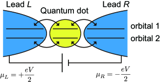
Figure 1: A schematic of a quantum dot connected to left and right lead electrodes with orbital degrees of freedom. Bias voltage $eV$ is applied between the two lead electrodes. In electron tunneling between the dot and the leads, the spin and orbital degrees of freedom are assumed to be conserved.

described by an Anderson impurity model:

$${\cal H}_{\rm A} = {\cal H}_{0}+{\cal H}_{\rm T}+{\cal H}_{\rm I}\,,$$ (1)

where

$${\cal H}_{0} = \sum_{\alpha m\sigma}\int_{-D}^{D}d\varepsilon\,\varepsilon\,c_{\varepsilon\alpha m\sigma}^{\dagger}c_{\varepsilon\alpha m\sigma}+\sum_{m\sigma}\epsilon_{\rm d}d_{m\sigma}^{\dagger}d_{m\sigma}\,,$$ (2)

$${\cal H}_{\rm T} = \sum_{\alpha m\sigma}\left[v_{\alpha}d_{m\sigma}^{\dagger}\psi_{\alpha m\sigma}+v_{\alpha}^{*}\psi_{\alpha m\sigma}^{\dagger}d_{m\sigma}\right]\,,$$ (3)

$${\cal H}_{\rm I} = U\sum_{m}\hat{n}_{{\rm d}m\uparrow}\hat{n}_{{\rm d}m\downarrow}+W\hat{n}_{{\rm d}1}\hat{n}_{{\rm d}2}+2J\hat{\bm{S}}_{{\rm d}1}\cdot\hat{\bm{S}}_{{\rm d}2}\,.$$ (4)

The first term ${\cal H}_{0}$ represents electrons in the two lead electrodes and the quantum dot. The operator $c_{\alpha\epsilon m\sigma}$ annihilates an electron with spin $\sigma=\uparrow,\downarrow$, orbital $m=1,2$ and energy $\varepsilon$ in the conduction band of the left and right electric leads $\alpha=L,R$. The operator $d_{m\sigma}$ annihilates an electron with spin $\sigma$ and orbital $m$ in the dot level $\epsilon_{\rm d}$. The second term ${\cal H}_{\rm T}$ represents the electron tunneling between the leads and the dot. The leads and the dot are connected by tunneling matrix element $v_{\alpha}$ through $\psi_{\alpha m\sigma}:=\int_{-D}^{D}d\varepsilon\sqrt{\rho_{\rm c}}c_{\varepsilon\alpha m\sigma}$ where $D$ is the half width of the conduction band and $\rho_{\rm c}=\frac{1}{2D}$ is the density of state for the conduction electrons. The electron tunneling leads to an intrinsic linewidth of the dot level given by $\Gamma=\frac{1}{2}\left(\Gamma_{L}+\Gamma_{R}\right)$ with $\Gamma_{\alpha}:=2\pi\rho_{\rm c}\left|v_{\alpha}\right|^{2}$. The last term ${\cal H}_{\rm I}$ represents the interaction between the electrons in the dot, where $U$ and $W$ are the intra- and interorbital Coulomb interaction, respectively, and $J$ is the exchange interaction. The number operators of the electrons in the dot are defined by $\hat{n}_{{\rm d}m\sigma}:=d_{m\sigma}^{\dagger}d_{m\sigma}$ and $\hat{n}_{{\rm d}m}:=\sum_{\sigma}\hat{n}_{{\rm d}m\sigma}$, and the total spin operator for the electrons in the dot in channel $m$ is defined by $\hat{\bm{S}}_{{\rm d}m}:=\sum_{\sigma\sigma^{\prime}}d_{m\sigma}^{\dagger}{\bm{\sigma}}_{\sigma\sigma^{\prime}}d_{m\sigma^{\prime}}$, where ${\bm{\sigma}}$ is the Pauli matrix.

In calculation of current correlations, we assume particle-hole symmetric $\epsilon_{\rm d}=-\frac{U}{2}-W$, symmetric connection $\Gamma_{L}=\Gamma_{R}$, and the absolute zero temperature $T=0$ to eliminate thermal and partition noise and emphasize spin-entanglement due to the exchange interaction $J$. The bias voltage $eV$ is symmetrically applied between the left and right leads to induce electric current: The chemical potential of the left and right leads are $\mu_{L}=+\frac{1}{2}eV$ and $\mu_{R}=-\frac{1}{2}eV$, respectively. Without loss of generality, positive bias voltage $eV>0$ can be taken. We also use the natural unit $\hbar=k_{\rm B}=e=1$.

We investigate spin entanglement of interacting quasiparticle pairs emerging in nonlinear currents through the two orbitals, exploiting cross-correlations for current with two twisted spin angles. The operator of the electric current with spin angled to the $\theta$ direction, from the lead $\alpha$ to the dot can be defined by

$$I_{\alpha m\theta}=-i\left(v_{\alpha}d_{m\theta}^{\dagger}\psi_{\alpha m\theta}-v_{\alpha}^{*}\psi_{\alpha m\theta}^{\dagger}d_{m\sigma}\right)\,.$$ (5)

Here the operators for the electrons with spin angled to the $\theta$ direction can be defined by a rotational transformation without loss of generality:

$$\begin{pmatrix}d_{m\theta}\\ d_{m\,\theta+\pi}\end{pmatrix} := \begin{pmatrix}\cos\frac{\theta}{2}&-\sin\frac{\theta}{2}\\ \sin\frac{\theta}{2}&\cos\frac{\theta}{2}\end{pmatrix}\begin{pmatrix}d_{m\uparrow}\\ d_{m\downarrow}\end{pmatrix}\,,$$ (6)

$$\begin{pmatrix}\psi_{\alpha m\theta}\\ \psi_{\alpha m\,\theta+\pi}\end{pmatrix} := \begin{pmatrix}\cos\frac{\theta}{2}&-\sin\frac{\theta}{2}\\ \sin\frac{\theta}{2}&\cos\frac{\theta}{2}\end{pmatrix}\begin{pmatrix}\psi_{\alpha m\uparrow}\\ \psi_{\alpha m\downarrow}\end{pmatrix}\,.$$ (7)

We note that our analysis can be applied to not only single quantum dots with orbital degeneracy Sasaki et al. (2004); Jarillo-Herrero et al. (2005) but also double quantum dots with two current channels. Keller et al. (2014)

II.2 Renormalized perturbation theory

To derive the precise form of current cross-correlations under the electron correlations of the Anderson impurity model at low energies, we make use of the renormalized perturbation theory.

The renormalized perturbation theory is an idea to reorganize the series of perturbation expansion, which is very useful for systems where the renormalization effect strongly acts such as Kondo impurities. The renormalized perturbation theory for the Anderson impurity model links the microscopic local Fermi liquid theory where perturbation expansion is done in powers of bare interactions Yamada (1975); Yoshimori (1976) to phenomenological local Fermi liquid theory where perturbation expansion is done in powers of the renormalized interactions. Nozières (1974) Thus, the theory tells us the precise way to calculate currents and current-correlations at low energies, by perturbation expansion in the renormalized interactions, and brings an intuitive understanding of the current due to low-lying excited states in the quasiparticle picture.

In this subsection, we illustrate the renormalized perturbation theory for the Anderson impurity model with degenerate orbitals given by Eq. (1). Hewson (1993b, 2001); Nishikawa et al. (2010) Then, we apply this theory to calculate current cross-correlations up to third order in bias-voltage $V^{3}$. The basic idea is as the following. In the local Fermi liquid region, perturbation expansion in the interactions $U,W$, and $J$ for all orders gives the exact result at low energies. However, it is very difficult, except for some special cases, to calculate all series in the perturbation expansion. Here, employing the idea of the renormalized perturbation theory, we reorganize the perturbation expansion and effectively carry out all-order calculation at low energies.

Let us start with the partition function for the Anderson impurity model given by Eq. (1), which can be expressed as a functional integral over time-dependent Grassmann variables along the Keldysh contour $C$ [see Fig. 2 (a)],

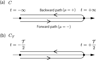
Figure 2: The Keldysh contour (a) $C$ between $t=-\infty$ and $t=+\infty$, and (b) $C_{\cal T}$ between $t=-\frac{\cal T}{2}$ and $t=+\frac{\cal T}{2}$. The indices $\mu=-$ and $+$ specify the forward and backward paths, respectively.

$${\cal Z}=\int\prod_{\alpha m\sigma}{\cal D}\left(\bar{d}_{m\sigma}\right){\cal D}\left(d_{m\sigma}\right){\cal D}\left(\bar{c}_{\varepsilon\alpha m\sigma}\right){\cal D}\left(c_{\varepsilon\alpha m\sigma}\right)e^{i{\cal S}}\,,$$

where the action is given by

$${\cal S}=\sum_{\mu}\int_{-\infty}^{\infty}dt\,\left(\sigma_{3}\right)^{\mu\mu}{\cal L}_{\rm A}^{\mu}(t).$$ (9)

with

$$\sigma_{3}=\begin{pmatrix}1&0\\ 0&-1\end{pmatrix}.$$ (10)

The superscripts $\mu=-$ and $+$ label the forward and backward paths of the Keldysh contour, respectively, as shown in Fig. 2 (a). The integral along the Keldysh contour allows us to calculate expectation values in nonequilibrium states. Our Anderson impurity model in the Lagrangean form is given by

$${\cal L}_{\rm A}^{\mu}(t)={\cal L}_{0}^{\mu}(t)+{\cal L}_{\rm T}^{\mu}(t)+{\cal L}_{\rm I}^{\mu}(t)\,,$$ (11)

with

$${\cal L}_{0}^{\mu}(t) = \sum_{\alpha m\sigma}\int_{-D}^{D}d\varepsilon\,\bar{c}_{\varepsilon\alpha m\sigma}^{\mu}(t)\left(i\frac{\partial}{\partial t}-\varepsilon\right)c_{\varepsilon\alpha m\sigma}^{\mu}(t)$$ (12)

$$\qquad+\sum_{m\sigma}\bar{d}_{m\sigma}^{\mu}(t)\left(i\frac{\partial}{\partial t}-\epsilon_{\rm d}\right)d_{m\sigma}^{\mu}(t)\,,$$

$${\cal L}_{\rm T}^{\mu}(t) = \sum_{\alpha m\sigma}\left[v_{\alpha}\bar{d}_{m\sigma}^{\mu}(t)\,\psi_{\alpha m\sigma}^{\mu}(t)\right.$$ (13)

$$\qquad\left.+v_{\alpha}^{*}\bar{\psi}_{\alpha m\sigma}^{\mu}(t)\,d_{m\sigma}^{\mu}(t)\right]\,,$$

$${\cal L}_{\rm I}^{\mu}\left(t\right) = U\sum_{m}n_{{\rm d}m\uparrow}^{\mu}(t)\,n_{{\rm d}m\downarrow}^{\mu}(t)$$ (14)

$$+Wn_{{\rm d}1}^{\mu}(t)\,n_{{\rm d}2}^{\mu}(t)+2J{\bm{S}}_{{\rm d}1}^{\mu}(t)\cdot{\bm{S}}_{{\rm d}2}^{\mu}(t)\,.$$

Here, the Grassmann numbers are defined by

$$n_{{\rm d}m\sigma}^{\mu}(t) := \bar{d}_{m\sigma}^{\mu}(t)d_{m\sigma}^{\mu}(t)\,,$$ (15)

$$n_{{\rm d}m}^{\mu}(t) := \sum_{sigma}n_{{\rm d}m\sigma}^{\mu}(t)\,,$$ (16)

$${\bm{S}}_{{\rm d}m}^{\mu}(t) := \sum_{\sigma\sigma^{\prime}}\bar{d}_{m\sigma}^{\mu}(t){\bm{\sigma}}_{\sigma\sigma^{\prime}}d_{m\sigma^{\prime}}^{\mu}(t)\,,$$ (17)

$$\psi_{\alpha m\sigma}^{\mu}(t) := \int_{-D}^{D}d\varepsilon\sqrt{\rho_{\rm c}}c_{\varepsilon\alpha m\sigma}^{\mu}(t),$$ (18)

$$\bar{\psi}_{\alpha m\sigma}^{\mu}(t) := \int_{-D}^{D}d\varepsilon\sqrt{\rho_{\rm c}}\bar{c}_{\varepsilon\alpha m\sigma}^{\mu}(t).$$ (19)

On introducing a self-energy $\Sigma_{{\rm d}m\sigma}^{\rm r}(\omega)$ due to the interactions, $U,W$, and $J$, the full retarded Green’s function for the electrons in the dot can be written in the form

$$G_{{\rm d}m\sigma}^{\rm r}(\omega)=\frac{1}{\omega-\epsilon_{\rm d}+i\Gamma-\Sigma_{{\rm d}m\sigma}^{\rm r}(\omega)}\,.$$ (20)

We reorganize the perturbation expansion in the bare interactions $U,W$, and $J$ to a form appropriate for the low energies. The first step is to write the self-energy in the form

$$\Sigma_{{\rm d}m\sigma}^{\rm r}(\omega)=\Sigma_{{\rm d}m\sigma}^{\rm r}(0)+\omega\,\Sigma_{{\rm d}m\sigma}^{{\rm r}\,\prime}(0)+\Sigma_{{\rm d}m\sigma}^{\rm rem}(\omega)\,,$$ (21)

which defines the remainder self-energy $\Sigma_{{\rm d}m\sigma}^{\rm rem}(\omega)$. Here, $\Sigma_{{\rm d}m\sigma}^{{\rm r}\,\prime}(\omega):=\frac{\partial\Sigma_{{\rm d}m\sigma}^{\rm r}(\omega)}{\partial\omega}$. Substituting the self-energy in this form into the full Green’s function given in Eq. (20), Green’s function of the quasiparticles $\widetilde{G}_{{\rm d}m\sigma}^{\rm r}\left(\omega\right)$ takes the same form with a renormalized energy level of the localized state $\tilde{\epsilon}_{\rm d}:=z\left[\epsilon_{\rm d}+\Sigma_{{\rm d}m\sigma}^{\rm r}(0)\right]$, level width $\widetilde{\Gamma}:=z\Gamma$, and self-energy $\widetilde{\Sigma}_{{\rm d}m\sigma}^{\rm r}(\omega):=z\Sigma_{{\rm d}m\sigma}^{\rm rem}(\omega)$:

$$G_{{\rm d}m\sigma}^{\rm r}(\omega) = \frac{z}{\omega-\tilde{\epsilon}_{\rm d}+i\widetilde{\Gamma}-\widetilde{\Sigma}_{{\rm d}m\sigma}^{\rm r}(\omega)}$$ (22)

$$= z\widetilde{G}_{{\rm d}m\sigma}^{\rm r}(\omega)\,.$$ (23)

Here, the wave function renormalization factor is defined by $z:=\left[1-\Sigma_{{\rm d}m\sigma}^{{\rm r}\,\prime}(0)\right]^{-1}$. The renormalized linewidth $\widetilde{\Gamma}$ corresponds to the characteristic energy scale, namely, the Kondo temperature as $T_{\rm K}=\pi\widetilde{\Gamma}/4$. We note that $\Sigma_{{\rm d}m\sigma}^{\rm r}(0)$ and $\Sigma_{{\rm d}m\sigma}^{{\rm r}\,\prime}(0)$ are to be evaluated at $\omega=0,T=0$, and $V=0$. The overall factor $z$ in Green’s function is removed by rescaling the Grassmann numbers of the dot state as, $d_{m\sigma}=\sqrt{z}\tilde{d}_{m\sigma}$ and $\bar{d}_{m\sigma}=\sqrt{z}\tilde{\bar{d}}_{m\sigma}$.

The last parameters specifying the renormalized theory are the renormalized interactions $\widetilde{U},\widetilde{W}$, and $\widetilde{J}$. These quantities are derived from the four-point vertex function $\Gamma_{m_{3}\sigma_{3};m_{4}\sigma_{4}}^{m_{1}\sigma_{1};m_{2}\sigma_{2}}(\omega_{1},\omega_{2},\omega_{3},\omega_{4})$, which is derived from the time-ordering two-particles Green’s function of the dot electrons at $V=0$ and $T=0$. The renormalized four-vertex is defined by

$$\widetilde{\Gamma}_{m_{3}\sigma_{3};m_{4}\sigma_{4}}^{m_{1}\sigma_{1};m_{2}\sigma_{2}}\left(\omega_{1},\omega_{2},\omega_{3},\omega_{4}\right)$$

$$\qquad:=z^{2}\Gamma_{m_{3}\sigma_{3};m_{4}\sigma_{4}}^{m_{1}\sigma_{1};m_{2}\sigma_{2}}\left(\omega_{1},\omega_{2},\omega_{3},\omega_{4}\right)\,,$$ (24)

through the rescaling of four fermion fields for the dot site. The renormalized interactions are then defined by the value of the four-vertex at $\omega_{1}=\omega_{2}=\omega_{3}=\omega_{4}=0$:

$$z^{2}\Gamma_{m_{3}\sigma_{3};m_{4}\sigma_{4}}^{m_{1}\sigma_{1};m_{2}\sigma_{2}}\left(0,0,0,0\right)$$

$$\qquad=:\left[\left(\widetilde{U}+\widetilde{J}\right)\delta_{m_{2}}^{m_{1}}+\left(\widetilde{W}-\frac{\widetilde{J}}{2}\right)\left(1-\delta_{m_{2}}^{m_{1}}\right)\right]$$

$$\qquad\qquad\qquad\times\left(\delta_{m_{4}}^{m_{1}}\delta_{m_{3}}^{m_{2}}\delta_{\sigma_{4}}^{\sigma_{1}}\delta_{\sigma_{3}}^{\sigma_{2}}-\delta_{m_{3}}^{m_{1}}\delta_{m_{4}}^{m_{2}}\delta_{\sigma_{3}}^{\sigma_{1}}\delta_{\sigma_{4}}^{\sigma_{2}}\right)$$

$$\qquad\qquad-\widetilde{J}\left(\delta_{m_{3}}^{m_{1}}\delta_{m_{4}}^{m_{2}}\delta_{\sigma_{4}}^{\sigma_{1}}\delta_{\sigma_{3}}^{\sigma_{2}}-\delta_{m_{4}}^{m_{1}}\delta_{m_{3}}^{m_{2}}\delta_{\sigma_{3}}^{\sigma_{1}}\delta_{\sigma_{4}}^{\sigma_{2}}\right)\,,$$ (25)

where $\delta_{m_{2}}^{m_{1}}$ is the Kronecker’s delta.

The quasiparticle’s Lagrangean $\widetilde{\cal L}_{\rm qp}^{\mu}(t)$ to describe properties at low energies is obtained by replacing the parameters of the dot state of the Anderson impurity model given by Eq. (1) to the renormalized ones:

$$\widetilde{\cal L}_{\rm qp}^{\mu}(t) = \widetilde{\cal L}_{0}^{\mu}(t)+\widetilde{\cal L}_{\rm T}^{\mu}(t)+\widetilde{\cal L}_{\rm I}^{\mu}(t)\,,$$ (26)

where

$$\widetilde{\cal L}_{0}^{\mu}\left(t\right) = \sum_{\alpha m\sigma}\int_{-D}^{D}d\varepsilon\,\bar{c}_{\varepsilon\alpha m\sigma}^{\mu}\left(t\right)\left(i\frac{\partial}{\partial t}-\varepsilon\right)c_{\varepsilon\alpha m\sigma}^{\mu}\left(t\right)$$ (27)

$$\qquad+\sum_{m\sigma}\tilde{\bar{d}}_{m\sigma}^{\mu}\left(t\right)\left(i\frac{\partial}{\partial t}-\tilde{\epsilon}_{\rm d}\right)\tilde{d}_{m\sigma}^{\mu}\left(t\right)\,,$$

$$\widetilde{\cal L}_{\rm T}^{\mu}\left(t\right) = \sum_{\alpha m\sigma}\left[\tilde{v}_{\alpha}\tilde{\bar{d}}_{m\sigma}^{\mu}\left(t\right)\psi_{\alpha m\sigma}^{\mu}\left(t\right)\right.$$ (28)

$$\qquad\left.+\tilde{v}_{\alpha}^{*}\bar{\psi}_{\alpha m\sigma}^{\mu}\left(t\right)\tilde{d}_{m\sigma}^{\mu}\left(t\right)\right]\,,$$

$$\widetilde{\cal L}_{\rm I}^{\mu}\left(t\right) = \widetilde{U}\sum_{m}\tilde{n}_{{\rm d}m\uparrow}^{\mu}\left(t\right)\tilde{n}_{{\rm d}m\downarrow}^{\mu}\left(t\right)$$ (29)

$$+\widetilde{W}\tilde{n}_{{\rm d}1}^{\mu}\left(t\right)\tilde{n}_{{\rm d}2}^{\mu}\left(t\right)+2\widetilde{J}\widetilde{\bm{S}}_{{\rm d}1}^{\mu}\left(t\right)\cdot\widetilde{\bm{S}}_{{\rm d}2}^{\mu}\left(t\right)\,,$$

with

$$\tilde{v}_{\alpha} := \sqrt{z}v_{\alpha}\,,$$ (30)

$$\tilde{n}_{{\rm d}m\sigma}^{\mu}(t) := \tilde{\bar{d}}_{m\sigma}^{\mu}(t)\tilde{d}_{m\sigma}^{\mu}(t)\,,$$ (31)

$$\tilde{n}_{{\rm d}m}^{\mu}(t) := \sum_{\sigma}\tilde{n}_{{\rm d}m\sigma}^{\mu}(t)\,,$$ (32)

$$\widetilde{\bm{S}}_{{\rm d}m}^{\mu}(t) := \sum_{\sigma\sigma^{\prime}}\tilde{\bar{d}}_{m\sigma}^{\mu}(t){\bm{\sigma}}_{\sigma\sigma^{\prime}}\tilde{d}_{m\sigma^{\prime}}^{\mu}(t)\,.$$ (33)

As a part of the interaction effects are taken into account ab initio in the quasiparticle’s Lagrangean, compensating terms have to be introduced to avoid overcounting in the perturbation expansion. Then, the total Lagrangean has to be satisfied with

$${\cal L}_{\rm A}^{\mu}(t)=\widetilde{\cal L}_{\rm qp}^{\mu}(t)+{\cal L}_{\rm CT}^{\mu}(t).$$ (34)

Therefore, the specific form of the counter-term Lagrangean is given by

$${\cal L}_{\rm CT}^{\mu}(t) = \sum_{m\sigma}\tilde{\bar{d}}_{m\sigma}^{\mu}(t)\left(\xi_{1}i\frac{\partial}{\partial t}+\xi_{2}\right)\tilde{d}_{m\sigma}^{\mu}(t)$$ (35)

$$+\xi_{3}^{U}\sum_{m}\tilde{n}_{{\rm d}m\uparrow}^{\mu}(t)\,\tilde{n}_{{\rm d}m\downarrow}^{\mu}(t)+\xi_{3}^{W}\tilde{n}_{{\rm d}1}^{\mu}(t)\,\tilde{n}_{{\rm d}2}^{\mu}(t)$$

$$+2\xi_{3}^{J}\widetilde{\bm{S}}_{{\rm d}1}^{\mu}(t)\cdot\widetilde{\bm{S}}_{{\rm d}2}^{\mu}(t)\,.$$

In the reorganized perturbation theory, the action can be written in the terms of the quasiparticles. After formally integrating over the Grassmann numbers for the conduction electrons, the reduced action is given by

$${\cal S} = \sum_{\mu}\int_{-\infty}^{\infty}dt\left(\sigma_{3}\right)^{\mu\mu}\left[\widetilde{\cal L}_{\rm qp}^{\mu}\left(t\right)+{\cal L}_{\rm CT}^{\mu}(t)\right]$$ (37)

$$= \int_{-\infty}^{\infty}dt\int_{-\infty}^{\infty}dt^{\prime}\sum_{m\sigma}\tilde{\bar{\bm{d}}}_{m\sigma}(t)\left[\widetilde{\bm{g}}_{{d}m\sigma}(t-t^{\prime})\right]^{-1}\tilde{\bm{d}}_{m\sigma}(t^{\prime})$$

$$\qquad+\sum_{\mu}\left(\sigma_{3}\right)^{\mu\mu}\int_{-\infty}^{\infty}dt\,\left[\widetilde{\cal L}_{\rm I}^{\mu}(t)+{\cal L}_{\rm CT}^{\mu}(t)\right]$$

with

$$\tilde{\bar{\bm{d}}}(t)=\begin{pmatrix}\tilde{d}_{{\rm d}m\sigma}^{-}(t)&\tilde{d}_{{\rm d}m\sigma}^{+}(t)\end{pmatrix},\ \tilde{\bm{d}}(t)=\begin{pmatrix}\tilde{d}_{{\rm d}m\sigma}^{-}(t)\\ \tilde{d}_{{\rm d}m\sigma}^{+}(t)\end{pmatrix},$$ (38)

$$\widetilde{\bm{g}}_{{\rm d}m\sigma}(t)=\begin{pmatrix}\tilde{g}_{{\rm d}m\sigma}^{--}(t)&\tilde{g}_{{\rm d}m\sigma}^{-+}(t)\\ \tilde{g}_{{\rm d}m\sigma}^{+-}(t)&\tilde{g}_{{\rm d}m\sigma}^{++}(t)\end{pmatrix}\,.$$ (39)

Here, $\widetilde{\bm{g}}_{{\rm d}m\sigma}(t)$ is Green’s function of the free quasiparticle (see Appendix B). The coefficients of the counter terms, $\xi_{1},\xi_{2},\xi_{3}^{U},\xi_{3}^{W}$, and $\xi_{3}^{J}$, are expressed in powers of the renormalized interactions $\widetilde{U},\widetilde{W}$ and $\widetilde{J}$, which are determined by the renormalized condition for the renormalized self-energy given $\widetilde{\Sigma}_{{\rm d}m\sigma}^{\rm r}(0)=0$ and $\left.\frac{\partial\widetilde{\Sigma}_{{\rm d}m\sigma}^{\rm r}(0)}{\partial\omega}\right|_{\omega=0}=0$, and for the four-vertex $\widetilde{\Gamma}_{m_{3}\sigma_{3};m_{4}\sigma_{4}}^{m_{1}\sigma_{1};m_{2}\sigma_{2}}(0,0,0,0)$ (see Appendix A).

We can evaluate the values of the quasiparticle parameters, $\tilde{\epsilon}_{\rm d},\widetilde{\Gamma},\widetilde{U},\widetilde{W}$, and $\widetilde{J}$, with use of the numerical renormalization group approach, Hewson et al. (2004); Nishikawa et al. (2010, 2012a) because the quantities are defined at $T=0$ and $V=0$ (see Appendix C). The nonequilibrium effect at low bias voltages $V\ll T_{\rm K}\sim\widetilde{\Gamma}$ enters via perturbation expansion in the renormalized interactions.

The perturbation expansion up to only the second order in the renormalized interactions gives a precise expression of the self-energy at $T=0$ up to the second order in $\omega$ and $V$, and those of currents and current correlations up to order $V^{3}$. The counter terms cancel all the terms with higher orders in the renormalized interactions. Oguri (2005); Sakano et al. (2011a, b, 2012) We shall calculate current cross-correlation by the perturbation expansion in the renormalized interactions.

II.3 Full counting statistics

To calculate currents and current correlations, we make use of the full counting statistics. Bagrets et al. (2006); Esposito et al. (2009) There are two major advantages of the full counting statistics. One is that the technique gives all-order current correlations at once. The other is that labeled counting fields in the partition function classify scattering processes in the current, which provides us an intuitive understanding of the underlying physics of the currents and the current fluctuations. Thus, the combination of the renormalized perturbation expansion and the full counting statistics can be a powerful tool to explore the mechanism that leads to entangled states in the current.

Let us start with the probability distribution $P({\bm{q}})$ of the transferred charge

$${\bm{q}}=\left(q_{L1\uparrow},q_{L1\downarrow},q_{L2\uparrow},q_{L2\downarrow},q_{R1\uparrow},q_{R1\downarrow},q_{R2\uparrow},q_{R2\downarrow}\right)$$

with orbital $m$ spin $\sigma$ from lead $\alpha$ to the dot in a time interval ${\cal T}$ between $t=-\frac{\cal T}{2}$ and $t=\frac{\cal T}{2}$, which can provide the current correlation function to all orders. In this paper, we consider the steady currents in the long time limit ${\cal T}\to\infty$. For simplification of the spin subscript, $\sigma=\uparrow$ indicates spin angled to the $\theta(\phi)$ direction, and $\sigma=\downarrow$ indicates spin angled to the $\theta+\pi(\phi+\pi)$ direction for orbital $m=1(2)$, in the following. This probability distribution is given by

$$P({\bm{q}})=\left\langle\prod_{m\sigma\alpha}\delta_{\hat{n}_{\alpha m\sigma}\left(-\frac{\cal T}{2}\right)-\hat{n}_{\alpha m\sigma}\left(\frac{\cal T}{2}\right)}^{q_{\alpha m\sigma}}\right\rangle\,,$$ (40)

in terms of the operator for the number of charge in lead $\alpha$,

$$\hat{n}_{\alpha m\sigma}(t)=\int_{-D}^{D}d\varepsilon\,c_{\varepsilon\alpha m\sigma}^{\dagger}(t)\,c_{\varepsilon\alpha m\sigma}(t)\,.$$ (41)

The generation function for this probability distribution is given in the form

$$\chi\left({\bm{\lambda}}\right)=\sum_{\bm{q}}e^{i{\bm{\lambda}}\cdot{\bm{q}}}P\left({\bm{q}}\right)$$ (42)

with the counting field

$${\bm{\lambda}}=\left(\lambda_{L1\uparrow},\lambda_{L1\downarrow},\lambda_{L2\uparrow},\lambda_{L2\downarrow},\lambda_{R1\uparrow},\lambda_{R1\downarrow},\lambda_{R2\uparrow},\lambda_{R2\downarrow}\right).$$

The cumulant generating function can be written as

$$\ln\chi({\bm{\lambda}})=\ln{\cal Z}({\bm{\lambda}})\,,$$ (43)

in term of the partition function ${\cal Z}\left({\bm{\lambda}}\right)$ for an extended Lagrangean

$${\cal L}_{\rm A}^{\mu}(t,{\bm{\lambda}})={\cal L}_{0}^{\mu}(t)+{\cal L}_{\rm T}^{\mu}(t,{\bm{\lambda}})+{\cal L}_{\rm I}^{\mu}(t)\,.$$ (44)

This extended tunneling part is given by

$${\cal L}_{\rm T}^{\mu}(t,{\bm{\lambda}})=\sum_{\alpha m\sigma}\left[v_{\alpha}e^{i\lambda_{\alpha m\sigma}^{\mu}}d_{m\sigma}^{\dagger}(t)\psi_{\alpha m\sigma}(t)+{\rm H.c.}\right]\,,$$ (45)

where the sign of the counting field depends on the Keldysh contour as $\lambda_{\alpha m\sigma}^{\mu}=\left(\sigma_{3}\right)^{\mu\mu}\lambda_{m\sigma}$. Thus, the partition function is written in the path integral form:

$${\cal Z}({\bm{\lambda}})$$

$$=\int{\cal D}\left(\bar{c}_{\varepsilon\alpha m\sigma}\right){\cal D}\left(c_{\varepsilon\alpha m\sigma}\right){\cal D}\left(\bar{d}_{m\sigma}\right){\cal D}\left(d_{m\sigma}\right)e^{i{\cal S}({{\bm{\lambda}}})}\,,$$

where the action is given by

$${\cal S}({\bm{\lambda}}) = \int_{C_{\cal T}}dt\,{\cal L}_{\rm A}^{\mu}(t,{\bm{\lambda}})\,,$$ (47)

and $C_{\cal T}$ is a Keldysh contour in a time interval ${\cal T}$ [see Fig. 2(b)]. The counting field is introduced such that the terms where one electron moves from the left or right lead to the dot gain one counting field $e^{\lambda_{\alpha m\sigma}}$, as seen in the extended tunneling Lagrangean (45). It is useful for analyzing scattering processes in currents.

III Result and discussion

Let us calculate the cumulant generating function for the current through the quantum dot in the Kondo regime. Then, using the obtained cumulant generating function, current cross-correlations, averaged currents and shot noise, are derived in terms of renormalized parameters, and we investigate spin entanglement of quasiparticle pairs emerging in the current. Finally, we discuss interaction dependence of these quantities with use of the numerical renormalization group approach.

III.1 Cumulant generating function

Applying the renormalized perturbation theory, we can precisely include the local Fermi liquid properties in the partition function for low energies, which can be written in the quasiparticle picture as

$${\cal Z}({\bm{\lambda}})=\int{\cal D}\left(\tilde{\bar{d}}_{m\sigma}\right){\cal D}(\tilde{d}_{m\sigma})e^{i{\cal S}_{\rm red}({{\bm{\lambda}}})}\,,$$ (48)

where the reduced action is given by

$${\cal S}_{\rm red}({\bm{\lambda}})$$

$$=\int_{-\frac{\cal T}{2}}^{\frac{\cal T}{2}}dt\int_{-\frac{\cal T}{2}}^{\frac{\cal T}{2}}dt^{\prime}\sum_{m\sigma}\tilde{\bar{\bm{d}}}_{m\sigma}(t)\left[\widetilde{\bm{g}}_{{\rm d}m\sigma}^{\lambda}(t-t^{\prime})\right]^{-1}\tilde{\bm{d}}_{m\sigma}(t^{\prime})$$

$$\qquad+\sum_{\mu}\int_{-\frac{\cal T}{2}}^{\frac{\cal T}{2}}dt\,(\sigma_{3})^{\mu\mu}\left[\widetilde{\cal L}_{\rm I}^{\mu}(t)+\widetilde{\cal L}_{\rm CT}^{\mu}(t)\right]\,.$$ (49)

Here, $\widetilde{\bm{g}}_{{\rm d}m\sigma}^{\lambda}(t)$ is the Green’s function of the free quasiparticle with the counting fields (see Appendix B).

Applying the perturbation expansion in the renormalized interactions to the partition function given in Eq. (48), the cumulant generating function up to the third order in $V$ is precisely calculated in terms of the renormalized parameters:

$$\ln\chi({\bm{\lambda}}) = \ln{\chi}_{0}({\bm{\lambda}})+\frac{\cal T}{2\pi}V\left(\frac{V}{\widetilde{\Gamma}}\right)^{2}\left({\cal A}+{\cal B}\right)+{\cal O}(V^{5})\,.$$

This is a key result. Equation (LABEL:eq:CGF-2ndodr) enables us to calculate the current correlations in all orders by differentiating it with respect to the counting fields. It also describes the scattering processes of the low-energy excited states in the current. The first term of Eq. (LABEL:eq:CGF-2ndodr) describes the free-quasiparticles contribution, which is resulted from the zeroth order term of the perturbation expansion in the renormalized interaction as

$$\ln\chi_{0}({\bm{\lambda}})=\frac{{\cal T}}{2\pi}\sum_{m\sigma}\int_{-\frac{V}{2}}^{+\frac{V}{2}}d\omega\ln\left[1+T_{m\sigma}(\omega)\left(e^{i\bar{\lambda}_{m\sigma}}-1\right)\right]\,.$$

In the free-quasiparticle’s process, the quasiparticles are scattered by the resonant level near the Fermi level, described by the transmission probability

$$T_{m\sigma}(\omega)=-\Gamma{\rm Im}G_{{\rm d}m\sigma}^{\rm r}(\omega)=\frac{\widetilde{\Gamma}^{2}}{\omega^{2}+\widetilde{\Gamma}^{2}}\,.$$ (52)

The second term of Eq. (LABEL:eq:CGF-2ndodr) is obtained by second order calculation in the renormalized interactions as

$${\cal A} = \tilde{u}^{2}\left\{\frac{1}{12}\sum_{m\sigma}\left(e^{-i\bar{\lambda}_{m\sigma}}-1\right)+\frac{1}{3}\sum_{m}\left[e^{-i\left(\bar{\lambda}_{m\uparrow}+\bar{\lambda}_{m\downarrow}\right)}-1\right]\right\}$$ (53)

$$\qquad+\frac{1}{4}\tilde{j}^{2}\left[\cos^{2}\left(\theta-\varphi\right)+1\right]\left\{\frac{1}{24}\sum_{m\sigma}\sum_{m^{\prime}}^{m^{\prime}\neq m}\left[e^{-i\left(\lambda_{Rm\sigma}-\lambda_{Rm^{\prime}\sigma}-\lambda_{Rm\bar{\sigma}}+\lambda_{Lm^{\prime}\bar{\sigma}}\right)}-1\right]\right.$$

$$\qquad\qquad+\frac{1}{24}\sum_{m\sigma}\sum_{m^{\prime}}^{m^{\prime}\neq m}\left[e^{-i\left(\lambda_{Lm\sigma}+\lambda_{Lm^{\prime}\bar{\sigma}}-\lambda_{Lm\bar{\sigma}}-\lambda_{Rm^{\prime}\sigma}\right)}-1\right]+\left.\frac{1}{3}\sum_{\sigma}\left[e^{-i\left(\lambda_{L2\sigma}+\lambda_{L1\bar{\sigma}}-\lambda_{R1\sigma}-\lambda_{R2\bar{\sigma}}\right)}-1\right]\right\}$$

$$\qquad+\left[\tilde{w}-\frac{1}{2}\tilde{j}\cos\left(\theta-\varphi\right)\right]^{2}\left\{\frac{1}{6}\sum_{m\sigma}\left(e^{-i\bar{\lambda}_{m\sigma}}-1\right)+\frac{1}{3}\sum_{\sigma\sigma^{\prime}}\left[e^{-i\left(\bar{\lambda}_{1\sigma}+\bar{\lambda}_{2\sigma^{\prime}}\right)}-1\right]\right\}$$

$$\qquad+\tilde{j}\tilde{w}\cos\left(\theta-\varphi\right)\left\{\frac{1}{6}\sum_{m\sigma}\left(e^{-i\bar{\lambda}_{m\sigma}}-1\right)+\frac{2}{3}\sum_{\sigma}\left[e^{-i\left(\bar{\lambda}_{1\sigma}+\bar{\lambda}_{2\sigma}\right)}-1\right]\right\}\,,$$

$${\cal B} = \frac{1}{4}\tilde{j}^{2}\left[\cos\left(\theta-\varphi\right)-1\right]^{2}\sum_{\sigma}\left\{\frac{1}{3}\left[e^{-i\left(\lambda_{L1\sigma}+\lambda_{L2\sigma}-\lambda_{R1\bar{\sigma}}-\lambda_{R2\bar{\sigma}}\right)}-1\right]+\frac{1}{24}\left[e^{-i\left(\lambda_{R1\sigma}+\lambda_{L2\sigma}-\lambda_{R1\bar{\sigma}}-\lambda_{R2\bar{\sigma}}\right)}-1\right]\right.$$ (54)

$$\qquad\qquad+\frac{1}{24}\left[e^{-i\left(\lambda_{L1\sigma}+\lambda_{R2\sigma}-\lambda_{R1\bar{\sigma}}-\lambda_{R2\bar{\sigma}}\right)}-1\right]+\frac{1}{24}\left[e^{-i\left(\lambda_{L1\sigma}+\lambda_{L2\sigma}-\lambda_{R1\bar{\sigma}}-\lambda_{L2\bar{\sigma}}\right)}-1\right]$$

$$\qquad\qquad\left.+\frac{1}{24}\left[e^{-i\left(\lambda_{L1\sigma}+\lambda_{L2\sigma}-\lambda_{L1\bar{\sigma}}-\lambda_{R2\bar{\sigma}}\right)}-1\right]\right\}$$

$$\qquad+\frac{1}{4}\tilde{j}^{2}\sin^{2}\left(\theta-\varphi\right)\sum_{mm^{\prime}\sigma^{\prime}}\sum_{m^{\prime}}^{m^{\prime}\neq m}\left\{\frac{1}{3}\left[e^{i\left(\lambda_{Rm{\sigma}^{\prime}}+\lambda_{Rm^{\prime}{\sigma}}-\lambda_{Lm^{\prime}\bar{\sigma}}-\lambda_{Lm{\sigma}^{\prime}}\right)}-1\right]+\frac{1}{12}\left[e^{i\left(\lambda_{Rm{\sigma}}-\lambda_{Lm\bar{\sigma}}\right)}-1\right]\right.$$

$$\qquad\qquad\qquad\qquad\left.+\frac{1}{24}\left[e^{i\left(\lambda_{Rm{\sigma}^{\prime}}+\lambda_{Rm^{\prime}{\sigma}}-\lambda_{Rm^{\prime}\bar{\sigma}}-\lambda_{Lm{\sigma}^{\prime}}\right)}-1\right]+\frac{1}{24}\left[e^{i\left(\lambda_{Rm{\sigma}^{\prime}}+\lambda_{Lm^{\prime}{\sigma}}-\lambda_{Lm^{\prime}\bar{\sigma}}-\lambda_{Lm{\sigma}}\right)}-1\right]\right\}\,,$$

with $\bar{\sigma}=\uparrow\left(\downarrow\right)$ for $\sigma=\downarrow\left(\uparrow\right)$ and $\bar{\lambda}_{m\sigma}=\lambda_{Lm\sigma}-\lambda_{Rm\sigma}$. Here the renormalized interactions scaled by the renormalized linewidth, $\tilde{u}:=\frac{\widetilde{U}}{\pi\widetilde{\Gamma}},\tilde{w}:=\frac{\widetilde{W}}{\pi\widetilde{\Gamma}}$. and $\tilde{j}:=\frac{\widetilde{J}}{\pi\widetilde{\Gamma}}$, express the strengths of the interactions of the Fermi liquid. ${\cal A}$ and ${\cal B}$ represent the contribution of the interacting quasiparticles, and it is peculiar to nonequilibrium beyond the linear response current.

At the end of this subsection, we mention properties of the free-quasiparticle term. For low bias voltages, this term can be expanded in bias voltage $V$ up to the third order as

$$\ln\chi_{0}({\bm{\lambda}})$$

$$\ \sim\frac{\cal T}{2\pi}V\sum_{m\sigma}\left[i\bar{\lambda}_{m\sigma}-\frac{1}{12}\left(\frac{V}{\widetilde{\Gamma}}\right)^{2}\left(e^{-i\bar{\lambda}_{m\sigma}}-1\right)\right]$$

$$\qquad+{\cal O}(V^{5})\,.$$ (55)

This term does not contain any current correlations between the two orbitals. It is natural because this term is accounted for by the free quasiparticles. Therefore, only quasiparticles excited by the renormalized interactions in the nonlinear current of order $V^{3}$ can form spin-entanglement between the two channels.

We note that there is no current of order $V^{2}$ because of our setting of the particle-hole symmetry.

III.2 Current and current-correlations

Cross-correlation

We first calculate interorbital cross-correlations of current fluctuations, which can be readily derived as a derivative of Eq. (LABEL:eq:CGF-2ndodr) with respect to counting fields:

$$C_{\alpha\alpha}(\theta,\varphi) = \int_{-\infty}^{\infty}dt\ \left\langle\delta I_{\alpha 1\theta}(t)\,\delta I_{\alpha 2\varphi}(0)\right\rangle$$ (56)

$$= \frac{e^{2}}{\cal T}\left(-i\right)^{2}\left.\frac{\partial}{\partial\lambda_{\alpha 1\uparrow}}\frac{\partial}{\partial\lambda_{\alpha 2\uparrow}}\ln\chi({\bm{\lambda}})\right|_{{\bm{\lambda}}=0}$$

$$= B_{1}-B_{2}\cos(\theta-\varphi)+{\cal O}\left(V^{5}\right)$$

with

$$B_{1} = \frac{1}{2\pi}V\left(\frac{V}{\widetilde{\Gamma}}\right)^{2}\left(\frac{1}{4}\tilde{j}^{2}+\frac{1}{3}\tilde{w}^{2}\right)\,,$$ (57)

$$B_{2} = \frac{1}{2\pi}V\left(\frac{V}{\widetilde{\Gamma}}\right)^{2}\left(\frac{1}{4}\tilde{j}^{2}-\frac{1}{3}\tilde{w}\tilde{j}\right)\,.$$ (58)

Here, the operator of current fluctuation can be defined by $\delta I_{\alpha m\sigma}:=I_{\alpha m\sigma}-\left\langle I_{\alpha m\sigma}\right\rangle$. This is one of the main result of this paper. Here, the angle independent and dependent terms of Eq. (56) are related to the charge and spin correlation of excited particles and holes in the current, as following. The cross-correlation of charge currents and spin currents between orbitals $m=1$ and $2$ are given by

$$C_{\alpha\alpha}^{\rm c} = \int_{-\infty}^{\infty}dt\ \left\langle\delta I_{\alpha 1}^{\rm c}(t)\delta I_{\alpha 2}^{\rm c}(0)\right\rangle$$ (59)

$$= C_{\alpha\alpha}(\theta,\varphi)+C_{\alpha\alpha}(\theta+\pi,\varphi)$$

$$\quad+C_{\alpha\alpha}(\theta,\varphi+\pi)+C_{\alpha\alpha}(\theta+\pi,\varphi+\pi)$$

$$= 4B_{1}\,,$$

$$C_{\alpha\alpha}^{\rm s}(\theta,\varphi) = \int_{-\infty}^{\infty}dt\ \left\langle\delta I_{\alpha 1\theta}^{\rm s}(t)\delta I_{\alpha 2\varphi}^{\rm s}(0)\right\rangle$$ (60)

$$= C_{\alpha\alpha}(\theta,\varphi)-C_{\alpha\alpha}(\theta+\pi,\varphi)$$

$$\quad-C_{\alpha\alpha}(\theta,\varphi+\pi)+C_{\alpha\alpha}(\theta+\pi,\varphi+\pi)$$

$$= 4B_{2}\cos(\theta-\varphi)\,,$$

respectively. Here,

$$I_{\alpha m}^{\rm c} = \sum_{\sigma}I_{\alpha m\sigma}\,,$$ (61)

$$I_{\alpha m\theta}^{\rm s} = I_{\alpha m\theta}-I_{\alpha m\,\theta+\pi}\,,$$ (62)

are the charge and spin current, respectively. In our model, every single quasiparticle and hole carries both a charge and a spin. Thus, the ratio,

$$\frac{C_{\alpha\alpha}^{\rm s}\left(\theta,\varphi\right)}{C_{\alpha\alpha}^{\rm c}}=\frac{B_{2}}{B_{1}}\cos\left(\theta-\varphi\right)\,,$$ (63)

corresponds to the cross-correlation for effective spins per current-carrying charge. The prefactor is determined by the local-Fermi-liquid parameters, specifically the interorbital residual interactions $\tilde{w}$ and $\tilde{j}$ as,

$${\cal R}:=\frac{B_{2}}{B_{1}}=\frac{1-\frac{4}{3}\left(\frac{\tilde{w}}{\tilde{j}}\right)}{1+\frac{4}{3}\left(\frac{\tilde{w}}{\tilde{j}}\right)^{2}}\,.$$ (64)

Since ${\cal R}$ is the value of Eq. (63) for $\theta=\varphi$, positive (negative) values of ${\cal R}$ indicate that the charge pairs with the parallel (antiparallel) spins are dominant in the current.

We also find that the cross-correlation of the current with three different angular momenta is induced by the exchange interaction:

$$C_{\rm three} = \int dt\int dt^{\prime}\left\langle\delta I_{\alpha m\sigma}(t)\delta I_{\alpha m^{\prime}\sigma}(t^{\prime})\delta I_{\alpha m^{\prime}\bar{\sigma}}(0)\right\rangle$$ (65)

$$= \frac{(-i)^{3}}{\cal T}\left.\frac{\partial}{\partial\lambda_{\alpha m\sigma}}\frac{\partial}{\partial\lambda_{\alpha m^{\prime}\sigma}}\frac{\partial}{\partial\lambda_{\alpha m^{\prime}\bar{\sigma}}}\ln\chi({\bm{\lambda}})\right|_{{\bm{\lambda}}=0}$$

$$= \frac{1}{2\pi}\frac{1}{24}V\left(\frac{V}{\widetilde{\Gamma}}\right)^{2}\tilde{j}^{2}\,.$$

There is a cross-correlation of four different channels. However, it is equivalent to the above cross-correlation of three spin-orbit channels because of the conservation of the total angular momentum consisting of the spin and orbital angular momenta during the quasiparticle scattering processes by the residual interactions.

We shall demonstrate the existence of the spin-entanglement between the orbitals. The Lagrangean for quasiparticle’s interaction given by Eq. (29) can be rewritten in terms of the spin-singlet and triplet components:

$$\widetilde{\cal L}_{\rm I}^{\mu}(t) = \widetilde{U}\sum_{m}\tilde{n}_{{\rm d}m\uparrow}^{\mu}(t)\,\tilde{n}_{{\rm d}m\downarrow}^{\mu}(t)+\widetilde{W}\tilde{n}_{{\rm d}m}^{\mu}(t)\,\tilde{n}_{{\rm d}m}^{\mu}(t)$$ (66)

$$\quad-\frac{3\widetilde{J}}{2}\widetilde{J}\,\bar{b}_{\rm s}^{\mu}(t)\,b_{\rm s}^{\mu}(t)+\frac{\widetilde{J}}{2}\sum_{i=0,\pm}\bar{b}_{{\rm t}i}^{\mu}(t)\,b_{{\rm t}i}^{\mu}(t)\,,$$

where

$$\bar{b}_{\rm s}^{\mu}(t) = -\frac{1}{\sqrt{2}}\left[\tilde{\bar{d}}_{1\uparrow}^{\mu}(t)\tilde{\bar{d}}_{2\downarrow}^{\mu}(t)-\tilde{\bar{d}}_{1\downarrow}^{\mu}(t)\tilde{\bar{d}}_{2\uparrow}^{\mu}(t)\right]\,,$$

$$b_{\rm s}^{\mu}(t) = \frac{1}{\sqrt{2}}\left[\tilde{d}_{1\uparrow}^{\mu}(t)\tilde{d}_{2\downarrow}^{\mu}(t)-\tilde{d}_{1\downarrow}^{\mu}(t)\tilde{d}_{2\uparrow}^{\mu}(t)\right]\,,$$ (67)

$$\bar{b}_{{\rm t}0}^{\mu}(t) = -\frac{1}{\sqrt{2}}\left[\tilde{\bar{d}}_{1\uparrow}^{\mu}(t)\tilde{\bar{d}}_{2\downarrow}^{\mu}(t)+\tilde{\bar{d}}_{1\downarrow}^{\mu}(t)\tilde{\bar{d}}_{2\uparrow}^{\mu}(t)\right]\,,$$

$$b_{{\rm t}0}^{\mu}(t) = \frac{1}{\sqrt{2}}\left[\tilde{d}_{1\uparrow}^{\mu}(t)\tilde{d}_{2\downarrow}^{\mu}(t)+\tilde{d}_{1\downarrow}^{\mu}(t)\tilde{d}_{2\uparrow}^{\mu}(t)\right]\,,$$ (68)

$$\bar{b}_{{\rm t}+}^{\mu}(t) = -\tilde{\bar{d}}_{1\uparrow}^{\mu}(t)\tilde{\bar{d}}_{2\uparrow}^{\mu}(t)\,,\ b_{{\rm t}+}^{\mu}(t)=\tilde{d}_{1\uparrow}^{\mu}(t)\tilde{d}_{2\uparrow}^{\mu}(t)\,,$$ (69)

$$\bar{b}_{{\rm t}-}^{\mu}(t) = -\tilde{\bar{d}}_{1\downarrow}^{\mu}(t)\tilde{\bar{d}}_{2\downarrow}^{\mu}(t)\,,\ b_{{\rm t}-}^{\mu}(t)=\tilde{d}_{1\downarrow}^{\mu}(t)\tilde{d}_{2\downarrow}^{\mu}(t)\,,$$ (70)

are the Grassmann number for the spin-singlet and triplet states of two generated particles (holes) between the orbitals. Applying the perturbation expansion with respect to $\widetilde{\cal L}_{\rm I}^{\mu}(t)$, the term of the generating function with order $\widetilde{J}^{2}$ can be written by Green’s function for the singlet state and the triplet states:

$$\frac{\widetilde{J}^{2}}{4}\sum_{\mu\nu}(\sigma_{3})^{\mu\mu}(\sigma_{3})^{\nu\nu}\int_{-\frac{\cal T}{2}}^{+\frac{\cal T}{2}}dt\,dt^{\prime}\left[9\left\langle b_{\rm s}^{\mu}(t)\bar{b}_{\rm s}^{\nu}(t^{\prime})\right\rangle\left\langle\bar{b}_{\rm s}^{\mu}(t)b_{\rm s}^{\nu}(t^{\prime})\right\rangle+\sum_{i=0,1}\left\langle b_{{\rm t}i}^{\mu}(t)\bar{b}_{{\rm t}i}^{\nu}(t^{\prime})\right\rangle\left\langle\bar{b}_{{\rm t}i}^{\mu}(t)b_{{\rm t}i}^{\nu}(t^{\prime})\right\rangle\right]\,,$$ (71)

where

$$\left\langle\cdots\right\rangle=\frac{\int{\cal D}\left(\tilde{\bar{d}}_{m\sigma}\right){\cal D}(\tilde{d}_{m\sigma})\cdots e^{i{\cal S}_{\rm red}^{(0)}}}{\int{\cal D}\left(\tilde{\bar{d}}_{m\sigma}\right){\cal D}(\tilde{d}_{m\sigma})e^{i{\cal S}_{\rm red}^{(0)}}}$$ (72)

is an expectation value. Equation (71) shows that the spin entangled pairs given by Eqs. (67)-(70) are excited and result in the cross-correlation between the two currents. We note that there are additional $\widetilde{J}^{2}$ terms due to the counter term. However, they only eliminate the overcounting of the renormalization effect, and do not affect the form of the entangled pairs.

Averaged current

The average current in each channel of the right lead is also calculated from the first derivative of Eq. (LABEL:eq:CGF-2ndodr):

$$\left\langle I_{\alpha m\sigma}\right\rangle = \left.\frac{e}{\cal T}\left(-i\right)\frac{\partial}{\partial\lambda_{\alpha m\sigma}}\ln\chi\left({\bm{\lambda}}\right)\right|_{{\bm{\lambda}}=0}$$ (73)

$$= \left(1-2\delta_{\alpha}^{R}\right)\left(I_{u}-\left\langle I_{\alpha m\sigma}^{\rm NL}\right\rangle\right)\,,$$

where $I_{u}=\frac{1}{2\pi}V$ is the linear current, and

$$\left\langle I_{\alpha m\sigma}^{\rm NL}\right\rangle=\frac{1}{2\pi}\frac{1+5\widetilde{\cal I}}{12}V\left(\frac{V}{\widetilde{\Gamma}}\right)^{2}+{\cal O}\left(V^{5}\right)$$ (74)

is the nonlinear current with $\widetilde{\cal I}=\tilde{u}^{2}+2\tilde{w}^{2}+\frac{3}{2}\tilde{j}^{2}$. The averaged current is independent of the observation angles $\theta$ and $\varphi$.

Shot noise

The shot noise is a current noise due to the charge discretization, and is simply given by auto-correlation of the full current through the Anderson impurity. This is because the noise source is only a small amount of the scattering state of the excited quasiparticles by the renormalized interaction in the current. Thus, the shot noise is given by the second derivation with respect to the counting field as

$$S := \int dt\,\left\langle\delta I\left(t\right)\delta I\left(0\right)+\delta I\left(0\right)\delta I\left(t\right)\right\rangle$$ (75)

$$= \left(-i\right)^{2}\frac{2e^{2}}{\cal T}\left.\frac{\partial^{2}}{\partial\lambda^{2}}\ln\chi\left(\lambda\right)\right|_{\lambda=0}$$

$$= \frac{1}{3\pi}V\left(\frac{V}{\widetilde{\Gamma}}\right)^{2}\left(1+9\widetilde{\cal I}\right)\,,$$

where

$$\chi\left(\lambda\right)=\left.\chi\left({\bm{\lambda}}\right)\right|_{\lambda_{Lm\sigma}=-\lambda_{Rm\sigma}=\frac{\lambda}{2}}\,.$$ (76)

This form of the shot noise has already been derived for Hund’s rule exchange interaction $J<0$, Sakano et al. (2012) and here it is naturally extended to the whole of the local-Fermi-liquid region, including antiferromagnetic interaction $J>0$. The Fano factor for the backscattering current is given by the ratio of the shot noise and the nonlinear current as

$$F_{\rm b}:=\frac{S}{2e\left\langle I_{\alpha m\sigma}^{\rm NL}\right\rangle}=\frac{1+9\widetilde{\cal I}}{1+5\widetilde{\cal I}}.$$ (77)

The ratio of the current and its own shot noise usually gives an effective charge of the current-carrying state. However, a variety of quasiparticle-hole pairs are excited in the current owing to the continuous low-energy spectrum of the local Fermi-liquid, as seen in Eq. (LABEL:eq:CGF-2ndodr). In this case, the Fano factor can be defined as an average of the current-carrying effective charges $e_{i}^{*}(i=1,2,\cdots)$ of form Sela et al. (2006)

$$eF_{\rm b}=\frac{\sum_{i}\left\langle\left(e_{i}^{*}\right)^{2}\right\rangle}{\sum_{i}\left\langle e_{i}^{*}\right\rangle}.$$ (78)

In the remainder of this section, we investigate the interaction dependence of the transport quantities derived above, using the renormalized interactions calculated with the numerical renormalization group. In particular, we shall discuss behaviors of the transport quantities for ferromagnetic ($J<0$) and antiferromagnetic ($J>0$) exchange interactions.

III.3 Ferromagnetic exchange interaction

Figure 3 shows ${\cal R}$ as a function of ferromagnetic $J$ for four values of $W$ with $U$ fixed as $3.0\pi\Gamma$.

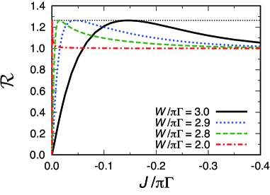
Figure 3: The value of ${\cal R}$ as a function of ferromagnetic $J(<0)$, with $U=3.0\pi\Gamma$, and several choices of $W=3.0\pi\Gamma,\,2.9\pi\Gamma,\,2.8\pi\Gamma$, and $2.0\pi\Gamma$. The thin dotted line indicates the maximum value ${\cal R}=\frac{1}{2}+\frac{\sqrt{21}}{6}=1.263\cdots$.

For $U=3.0\pi\Gamma$, the ground state stays in the Kondo regime, and it evolves continuously as $W$ and $J$ vary. The calculated renormalized interactions of the local Fermi liquid, $\tilde{u},\tilde{w}$, and $\tilde{j}$ are plotted in Fig. 4 as functions of bare ferromagnetic exchange interaction $J$.

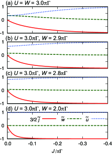
Figure 4: The renormalized interactions, $\tilde{j}$ (red solid line), $\tilde{u}$ (green dashed line), and $\tilde{w}$ (blue dotted line), as functions of ferromagnetic $J(<0)$, with $U=3.0\pi\Gamma$, and several choices of (a) $W=3.0\pi\Gamma$, (b) $W=2.9\pi\Gamma$, (c) $W=2.8\pi\Gamma$, and (d) $W=2.0$.

${\cal R}$ takes positive values for any finite strength of $J$, which indicates that the charge pairs with parallel spins are always dominant in the current. In the absence of the exchange interaction $J=0$, the renormalized one is also $\tilde{j}=0$ and thus no spin angle-dependent interactions are induced, while angle-independent renormalized interactions $\tilde{u}$ and $\tilde{w}$ are finite. As a result, $B_{2}=0$ while $B_{1}$ is finite, and the ratio becomes ${\cal R}=0$ at $J=0$. With increase of the strength of $J$, the spin entanglement between the two orbitals is enhanced. Then, ${\cal R}$ takes a common maximum $\frac{1}{2}+\frac{\sqrt{21}}{6}$ at a finite $J=J^{*}$ for any finite strength of $W$ with $U>W$. The two interorbital renormalized interactions, $\tilde{j}$ and $\tilde{w}$, cooperatively enhance the spin entanglement as the cross-term $\tilde{w}\tilde{j}$ arises in $B_{2}$. For larger ferromagnetic interaction $-J\gg\widetilde{\Gamma}\sim T_{\rm K}$ and $U>W$, the system crosses over to the $S=1$ full screening Kondo regime where the renormalized interactions take the universal values of the $S=1$ Kondo fixed point: $\tilde{u}\to 1,\tilde{w}\to 0$ , and $\tilde{j}\to-\frac{2}{3}$, as seen in Fig. 4. Nishikawa et al. (2010) In this limit, charge fluctuations due to the interorbital Coulomb interaction are suppressed, i.e., $\tilde{w}\to 0$, and the spin fluctuations are maximally enhanced, which results in

$${\cal R}\to 1\,.$$ (79)

We note that ${\cal R}=1$ does not mean that the current is fully spin-polarized. As seen in the generating function given in Eq. (LABEL:eq:CGF-2ndodr), correlated quasiparticles and holes excited by the exchange interaction give rise to pure spin current and charge current. Therefore, ${\cal R}=1$ simply means that the number of current-carrying spins is equal to that of charges.

The crossover from the SU(2) Kondo state for $U>W$ or the SU(4) Kondo state for $U=W$, and $J=0$ to the fully screened $S=1$ Kondo state at large strength of $J$, is observed in the ratio ${\cal R}$. Sakano et al. (2012) Note that, for $W=0$, the ratio is constant ${\cal R}=1$ for nonzero $J$, because the residual interorbital Coulomb interaction is always zero $\tilde{w}=0$, $\widetilde{W}=0$ in this case. As $-J$ increases, the renormalized interactions and ${\cal R}$ more rapidly converge to their own universal values for smaller values of $W$, because the Kondo temperature decreases with $W$.

This crossover through variation in the renormalized parameters can also be seen in the cross-correlation of three currents given by (65) and shot noise. The cross-correlation of three currents takes the form

$$C_{\rm three}=\frac{1}{2\pi}\frac{1}{864}V\left(\frac{\pi V}{T_{\rm K}}\right)^{2}$$ (80)

in the $S=1$ Kondo limit ($J/\Gamma\to-\infty$). The shot noise is also enhanced with the increase of two-particle backscattering due to the renormalized exchange interaction. This has been clearly seen in enhancement of the Fano factor. Sakano et al. (2012)

III.4 Antiferromagnetic interaction

Figures 5 and 6 show the computed values of ${\cal R}$, and the renormalized interactions, $\tilde{u},\,\tilde{w}$ and $\tilde{j}$, respectively, as a functions of ferromagnetic $J>0$ with $U=3\pi\Gamma$ and several values of $W$.

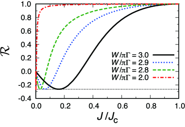
Figure 5: The values of ${\cal R}$ as a function of antiferromagnetic $J/J_{\rm c}$, with $U=3.0\pi\Gamma$, and several choices of (a) $W=3.0\pi\Gamma,\,2.9\pi\Gamma,\,2.8\pi\Gamma$, and $2.0\pi\Gamma$. $J$ is the normalized by the critical value $J_{\rm c}$ which is listed in Table 1. The thin dotted line indicates the minimum value ${\cal R}=\frac{1}{2}-\frac{\sqrt{21}}{6}=-0.263\cdots$.

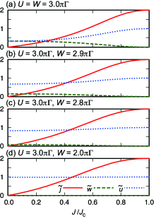
Figure 6: The renormalized interactions, $\tilde{j}$ (red solid line) $\tilde{u}$ (green dashed line) and $\tilde{w}$ (blue dotted line) as functions of antiferromagnetic $J/J_{\rm c}$, with $U=3.0\pi\Gamma$, and several choices of (a) $W=3.0\pi\Gamma$, (b) $W=2.9\pi\Gamma$, (c) $W=2.8\pi\Gamma$, and (d) $W=2.0\pi\Gamma$. The exchange interaction is normalized by the critical value $J_{\rm c}$ which is listed in Table 1.

There is a critical point at $J=J_{\rm c}$ for antiferromagnetic $J(>0)$. The values of the critical interaction $J_{\rm c}$ are listed in Table 1.

Table 1: The critical values $J_{\rm c}$ calculated by the numerical renormalization group, for $U=3.0\pi\Gamma$, and the values of $W$ used in Figs. 5 and 6.

$\frac{W}{\pi\Gamma}$	3.0	2.9	2.8	2.0
$\frac{J_{c}}{\pi\Gamma}$	0.1140	0.0950	0.08121	0.04034

For large antiferromagnetic interactions $J>J_{\rm c}$, two electrons occupied in the two orbitals form an isolated singlet state and decouple from the conduction electrons in the leads, and then no electric currents can flow through the quantum dot. Nishikawa et al. (2012a, b) Therefore, we focus on the region $J<J_{\rm c}$ where the low-energy state is accounted for by the local Fermi-liquid and electric current through the dot arises.

As the antiferromagnetic interaction increases, ${\cal R}$ decreases to a common and negative minimum $\frac{1}{2}-\frac{\sqrt{21}}{6}$, where cooperation of the interorbital interactions, $\tilde{w}$ and $\tilde{j}$, maximizes the number of the charge pairs with antiparallel spins in the current. Then, ${\cal R}$ turns to increases to the value ${\cal R}=1$ at the limit $J\to J_{\rm c}+0^{-}$ where the renormalized interactions take the values of $\tilde{u}\to 1,\tilde{w}\to 0$, and $\tilde{j}\to 2$ for $U>W$ Nishikawa et al. (2012a, b) as seen in Fig. 6. The number of the charge pairs with antiparallel spins decreases, and ones with parallel spins become dominant in the current. The excited state is described by Eq. (66) as long as the system stays in the local-Fermi-liquid region. Note that, for $W=0$, the ratio is unity for nonzero $J$, because the renormalized interorbital Coulomb interaction is always zero, $\tilde{w}=0$.

The crossover can also be seen in the cross-correlation of three currents given by (65) and the shot noise through variation in the renormalized parameters. The cross-correlation of three currents in the limit $J\to J_{\rm c}+0^{-}$ is given in a form

$$C_{\rm three}=\frac{1}{2\pi}\frac{1}{96}V\left(\frac{\pi V}{T_{\rm K}}\right)^{2}.$$ (81)

The Fano factor of the shot noise of the nonlinear current is shown in Fig. 7 as a function of $J$.

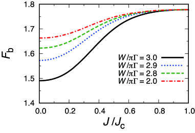
Figure 7: The Fano factor $F_{b}$, as a function of antiferromagnetic $J/J_{\rm c}(J>0)$, with $U=3.0\pi\Gamma$, and several choices of $W=3.0\pi\Gamma,\,2.9\pi\Gamma,\,2.8\pi\Gamma$, and $2.0\pi\Gamma$.

At the limit $J\to J_{\rm c}+0^{-}$, the Fano factors take a universal value

$$F_{\rm b}\to\frac{16}{9}.$$ (82)

By classifying the backscattered current by the effective charges, Sakano et al. (2012) the ratio of probability to generate current with effective charge $e$ and $2e$ are found to be 4:7, which result in the value through Eq. (78). Even near the critical point $J\to J_{\rm c}+0^{-}$, the Kondo effect or the Fermi liquid state with strong renormalization are held as the low energy state. Thus, $2e$ charge states are strongly backscattered in the current, which can be observed as an increase of $F_{\rm b}$. With an increase of $J$, the renormalized interactions, ${\cal R}$ and $F_{\rm b}$, more rapidly converge to their own universal values for smaller values of $W$, because the Kondo temperature decreases with $W$, similarly to the case with the ferromagnetic interaction.

IV Summary

We have investigated spin-entanglement of quasiparticle pairs excited by the renormalized interactions of the local Fermi liquid, which arise in nonlinear currents through the Kondo state of quantum dots with two degenerate orbitals and exchange interactions. We have shown, the cumulant generating function of the current is precisely described in the terms of the local Fermi-liquid parameters, up to third order in the applied bias voltage. Using this cumulant generating function, we have derived current correlations: cross-correlations between currents with two twisted spin in the different orbitals, cross-correlations of currents with three different spin-orbital channels, shot noises, and the Fano factor of the backscattering (nonlinear) currents. By calculating the renormalized parameters with use of the numerical renormalization group approach, we have investigated the exchange interaction dependence of these transport quantities. We have discussed spin-entanglement arising in the currents through two orbitals in current cross-correlations. It is elucidated that spin-angle dependent cross-correlation is induced by the exchange interactions.

Our approach can be extended to dots with more than two degenerate orbitals $N>2$. The low-energy state for the ferromagnetic exchange interaction is simply described by the $S=N/2$ Kondo state for any orbital degeneracy $N$ and the extension can be readily obtained. Sakano et al. (2012) However, discussion on the ground state for the antiferromagnetic exchange interaction contains more variety. For instance, the model for even $N$ has a critical interaction $J_{\rm c}$ and the conduction electrons decouple from the dot for $J>J_{\rm c}$, similarly to the case of $N=2$ discussed in the last section. Hattori and Tsunetsugu (2012) However, there is only one fixed point for odd $N$, where a degenerate ground state of the quantum dot due to the antiferromagnetic interaction yields the full-screened Kondo state. Futher explanation of this issue is beyond the scope of this paper.

Finally, further study on the spin entanglement of interacting quasiparticles in the currents may be done by the Bell’s inequality or the entanglement entropy. However, we note that not only particle pairs but also hole pairs and particle-hole pairs contribute to the spin entanglement as seen in the generating function, which makes it difficult to observe pure and individual entanglement of the quasiparticle pairs in the current.

Acknowldgement

RS thanks Shiro Kawabata and Taro Wakamura for helpful discussions and Yuya Shimazaki for inspiring discussions. This work was partially supported by JSPS KAKENHI Grant Nos. JP26220711, JP26400319, JP15K05181, and JP16K17723.

Appendix A Counter term

The coefficients of the counter term in Eq. (35) are formally determined by comparing both sides of Eq. (34) as an identity:

$$\xi_{1} = -\Sigma_{{\rm d}m\sigma}^{\rm r}(0)\,,$$ (83)

$$\xi_{2} = z-1\,,$$ (84)

$$\xi_{3}^{U} = z^{2}\left[U-\Gamma_{m\downarrow;m\uparrow}^{m\uparrow;m\downarrow}(0,0,0,0)\right]\,,$$ (85)

$$\xi_{3}^{W} = z^{2}\left\{W-\frac{1}{2}\left[\Gamma_{2\uparrow;1\uparrow}^{1\uparrow;2\uparrow}(0,0,0,0)+\Gamma_{2\downarrow;1\uparrow}^{1\uparrow;2\downarrow}(0,0,0,0)\right]\right\}\,,$$

$$\xi_{3}^{J} = z^{2}\left[J-\Gamma_{1\uparrow;2\downarrow}^{1\downarrow;2\uparrow}(0,0,0,0)\right]\,.$$ (87)

The specific form of the counter terms as series of the renormalized interactions for the particle-hole symmetric case $\epsilon_{\rm d}=-\frac{U}{2}-W$ can be calculated order by order. The coefficients of the counter term up to the second order in the renormalized interactions are obtained as

$$\xi_{1} = 0\,,$$ (88)

$$\xi_{2} = -\left(3-\frac{\pi^{2}}{4}\right)\widetilde{\cal I}+\cdots\,,$$ (89)

$$\xi_{3}^{U} = \pi\widetilde{\Gamma}\left[2\left(\tilde{w}-\frac{1}{2}\tilde{j}\right)^{2}-\tilde{j}^{2}\right]+\cdots\,,$$ (90)

$$\xi_{3}^{W} = \pi\widetilde{\Gamma}\tilde{u}\tilde{j}+\cdots\,,$$ (91)

$$\xi_{3}^{J} = \pi\widetilde{\Gamma}\left[-2\tilde{j}^{2}-2\tilde{u}\tilde{j}\right]+\cdots\,.$$ (92)

Most of the Fermi-liquid quantities can be written in the series of the renormalized interaction up to the second order. Therefore, this obtained form of the counter term allows us to calculate the precise and specific form of Fermi liquid quantities in terms of the renormalized parameters.

Appendix B Green’s function for free quasiparticle

The free-quasiparticle’s Green’s function in Eq. (37) is given by

$$\widetilde{\bm{g}}_{{\rm d}m\sigma}(t)=\int\frac{d\omega}{2\pi}\,\widetilde{\bm{g}}_{{\rm d}m\sigma}(\omega)\,e^{-i\omega t}\,.$$ (93)

with the four Keldysh component in $\omega$ space,

$$\tilde{g}_{{\rm d}m\sigma}^{--}(\omega) = \left[1-\widetilde{f}_{\rm eff}(\omega)\right]\tilde{g}_{{\rm d}m\sigma}^{\rm r}(\omega)+\widetilde{f}_{\rm eff}(\omega)\tilde{g}_{{\rm d}m\sigma}^{\rm a}(\omega)\,,$$

$$\tilde{g}_{{\rm d}m\sigma}^{-+}(\omega) = -\widetilde{f}_{\rm eff}(\omega)\left[\tilde{g}_{{\rm d}m\sigma}^{\rm r}(\omega)-\tilde{g}_{{\rm d}m\sigma}^{\rm a}(\omega)\right]\,,$$ (95)

$$\tilde{g}_{{\rm d}m\sigma}^{+-}(\omega) = \left[1-\widetilde{f}_{\rm eff}(\omega)\right]\left[\tilde{g}_{{\rm d}m\sigma}^{\rm r}(\omega)-\tilde{g}_{{\rm d}m\sigma}^{\rm a}(\omega)\right]\,,$$ (96)

$$\tilde{g}_{{\rm d}m\sigma}^{++}(\omega) = -\left[1-\widetilde{f}_{\rm eff}(\omega)\right]\tilde{g}_{{\rm d}m\sigma}^{\rm a}(\omega)-\widetilde{f}_{\rm eff}(\omega)\tilde{g}_{{\rm d}m\sigma}^{\rm r}(\omega)\,.$$

Here, the retarded and advanced Green’s function of the free quasiparticles are given by

$$\tilde{g}_{{\rm d}m\sigma}^{\rm r/a}(\omega)=\frac{1}{\omega-\tilde{\epsilon}_{\rm d}\pm i\widetilde{\Gamma}}$$ (98)

with the full linewidth $\widetilde{\Gamma}=\frac{1}{2}\left(\widetilde{\Gamma}_{L}+\widetilde{\Gamma}_{R}\right)$. The effective Fermi distribution function for the quasiparticles is given by

$$\widetilde{f}_{\rm eff}(\omega)=\frac{\widetilde{\Gamma}_{L}f_{L}(\omega)+\widetilde{\Gamma}_{R}f_{R}(\omega)}{\widetilde{\Gamma}_{L}+\widetilde{\Gamma}_{R}}\,,$$ (99)

where $f_{\alpha}(\omega)=\left[e^{\frac{\omega-\mu_{\alpha}}{T}}+1\right]^{-1}$ is the Fermi distribution function for the electrons in the isolated left and right leads.

The quasiparticle’s Green’s function with counting field in the $\omega$ space in Eq. (49) is given by

$$\tilde{g}_{{\rm d}m\sigma}^{\lambda--}(\omega) = \frac{1}{{\cal K}(\omega)}\left[\omega-\tilde{\epsilon}_{{\rm d}}-i\widetilde{\Gamma}+i\widetilde{\Gamma}\sum_{\alpha}f_{\alpha}(\omega)\right]\,,$$ (100)

$$\tilde{g}_{{\rm d}m\sigma}^{\lambda-+}(\omega) = \frac{-i\widetilde{\Gamma}}{{\cal K}(\omega)}\sum_{\alpha}e^{i\lambda_{\alpha m\sigma}}f_{\alpha}(\omega)\,,$$ (101)

$$\tilde{g}_{{\rm d}m\sigma}^{\lambda+-}(\omega) = \frac{i\widetilde{\Gamma}}{{\cal K}(\omega)}\sum_{\alpha}e^{-i\lambda_{\alpha m\sigma}}\left[1-f_{\alpha}(\omega)\right]\,,$$ (102)

$$\tilde{g}_{{\rm d}m\sigma}^{\lambda++}(\omega) = \frac{1}{{\cal K}(\omega)}\left[-\omega+\tilde{\epsilon}_{{\rm d}}+i\widetilde{\Gamma}-i\widetilde{\Gamma}\sum_{\alpha}f_{\alpha}(\omega)\right]\,,$$

where

$${\cal K}(\omega) = \left(\omega-\tilde{\epsilon}_{\rm d}\right)^{2}+\widetilde{\Gamma}^{2}$$ (104)

$$\ +\widetilde{\Gamma}^{2}\left[e^{-i\bar{\lambda}_{m\sigma}}-1\right]\left[1-f_{R}(\omega)\right]f_{L}(\omega)$$

with $\bar{\lambda}_{m\sigma}=\lambda_{Lm\sigma}-\lambda_{Rm\sigma}$.

Appendix C Calculation of renormalized parameters

Here we briefly show how to calculate values of $\tilde{\epsilon}_{\rm d},\widetilde{\Gamma},\widetilde{U},\widetilde{W}$, and $\widetilde{J}$, using the numerical renormalization group (NRG) approach. In this section, we fix the NRG iteration number $N$ close to the low energy fixed point and drop the $N$ dependencies from the expressions. The NRG eigen energy $E$ here is not multiplied by $\Lambda^{(N-1)/2}$, where $\Lambda$ is the logarithmic discretization parameter in NRG.

In our NRG calculation, the eigen energies are classified using a set of quantum number $(S,Q,\Delta Q)$, where $S$, $Q$, and $\Delta Q$ are the total spin, the total electron number and the difference in the number of electrons between the channels 1 and 2, respectively. We put ${\rm Spec}H_{S,Q,\Delta Q}:=\left\{{\rm NRG\ eigen\ energies\ labeled\ with}(S,Q,\Delta Q)\right\}$.

Near the low energy fixed point corresponding to the local Fermi-liquid state, the system is mainly described by the free quasiparticle Hamiltonian

$$H_{0}=\sum_{\kappa\eta n\sigma}{\mathcal{E}}^{(0)}_{\kappa,\eta,n}q^{\dagger}_{\kappa,\eta,n,\sigma}q_{\kappa,\eta,n,\sigma},$$ (105)

where $q_{\kappa,\eta,n,\sigma}$ annihilates a quasiparticle ($\kappa=1$) or quasihole ($\kappa=-1$) with spin $\sigma$ and $n$ th lowest energy in the channel 1 ($\eta=1$) or 2 ($\eta=-1$). We consider the lowest one-quasiparticle or one-quasihole excited state $q_{\kappa,\eta,{\rm 1st},\sigma}^{\dagger}|{\rm G}\rangle$ from the ground state $|{\rm G}\rangle$. This state is an eigen state of $H_{0}$ and has the eigen energy ${\mathcal{E}}^{(0)}_{\kappa,\eta,{\rm 1st}}$. Near the low energy fixed point, we can estimate the eigen energy as ${\mathcal{E}}^{(0)}_{\kappa,\eta,{\rm 1st}}=E^{(\rm 1st)}_{S_{\rm G}+\frac{1}{2},Q_{\rm G}+\kappa,\Delta Q_{G}+\kappa\eta}$, where $E^{(\rm 1st)}_{S,Q,\Delta Q}:={\rm min}{\rm Spec}H_{S,Q,\Delta Q}$ and $(S_{\rm G},Q_{\rm G},\Delta Q_{\rm G})$ is the set of quantum number of the ground state. (We usually have $S_{\rm G}=0$.)

Since ${\mathcal{E}}^{(0)}_{\kappa,\eta,{\rm 1st}}$ is determined by the poles of the Green’s function for the free quasiparticles, $\tilde{\epsilon}_{\rm d}$ and $\widetilde{\Gamma}$ can be deduced from NRG eigen energies:

$$\frac{1}{\widetilde{\Gamma}} = A_{\Lambda}\frac{2}{\pi}\frac{g_{00}\left(E^{(\rm 1st)}_{S_{\rm G}+\frac{1}{2},Q_{\rm G}+1,\Delta Q_{\rm G}+\eta}\right)-g_{00}\left(-E^{(\rm 1st)}_{S_{\rm G}+\frac{1}{2},Q_{\rm G}-1,\Delta Q_{\rm G}-\eta}\right)}{E^{(\rm 1st)}_{S_{\rm G}+\frac{1}{2},Q_{\rm G}+1,\Delta Q_{\rm G}+\eta}+E^{(\rm 1st)}_{S_{\rm G}+\frac{1}{2},Q_{\rm G}-1,\Delta Q_{\rm G}-\eta}},$$ (106)

$$\tilde{\epsilon}_{\rm d} = -A_{\Lambda}\tilde{\Gamma}\frac{2}{\pi}g_{00}\left(\kappa E^{(\rm 1st)}_{S_{\rm G}+\frac{1}{2},Q_{\rm G}+\kappa,\Delta Q_{\rm G}+\kappa\eta}\right),$$ (107)

where $g_{00}$ is the Green’s function at site $0$ for the NRG discretized chain of the conduction electrons and $A_{\Lambda}=\frac{1+1/\Lambda}{2(1-1/\Lambda)}\log\Lambda$ (For details, see Ref. Hewson et al., 2004.). There is a plateau in each of the graphs of $\tilde{\epsilon}_{\rm d}$ and $\widetilde{\Gamma}$ against $N$ toward the low energy fixed point, which enables us to determine the values of these renormalized parameters.

Next, we consider the following three two-quasiparticle excited states,

$$q_{\kappa,\eta,{\rm 1st},\uparrow}^{\dagger}q_{\kappa,\eta,{\rm 1st},\downarrow}^{\dagger}|{\rm G}\rangle\,,$$ (108)

$$q_{\kappa,+1,{\rm 1st},\uparrow}^{\dagger}q_{\kappa,-1,{\rm 1st},\uparrow}^{\dagger}|{\rm G}\rangle\,,$$ (109)

$$\frac{1}{\sqrt{2}}\left(q_{\kappa,+1,{\rm 1st},\uparrow}^{\dagger}q_{\kappa,-1,{\rm 1st},\downarrow}^{\dagger}-q_{\kappa,+1,{\rm 1st},\downarrow}^{\dagger}q_{k,-1,{\rm 1st},\uparrow}^{\dagger}\right)|{\rm G}\rangle.$$

The three states are eigen states of $H_{0}$, and the eigen energies are $2{\mathcal{E}}^{(0)}_{\kappa,\eta,{\rm 1st}}$,  ${\mathcal{E}}^{(0)}_{\kappa,+1,{\rm 1st}}+{\mathcal{E}}^{(0)}_{\kappa,-1,{\rm 1st}}$ and ${\mathcal{E}}^{(0)}_{\kappa,+1,{\rm 1st}}+{\mathcal{E}}^{(0)}_{\kappa,-1,{\rm 1st}}$, which are shifted by $\Delta E_{1}$,  $\Delta E_{2}$ and $\Delta E_{3}$, respectively, due to the renormalized interactions between the quasiparticles. Near the low energy fixed point, the three energy shifts can be evaluated using the NRG eigen energies:

$$\Delta E_{1} = E_{1}-2{\mathcal{E}}^{(0)}_{\kappa,\eta,{\rm 1st}}\,,$$ (111)

$$\Delta E_{2} = E_{2}-({\mathcal{E}}^{(0)}_{\kappa,+1,{\rm 1st}}+{\mathcal{E}}^{(0)}_{\kappa,-1,{\rm 1st}})$$ (112)

and

$$\Delta E_{3}=E_{3}-({\mathcal{E}}^{(0)}_{\kappa,+1,{\rm 1st}}+{\mathcal{E}}^{(0)}_{\kappa,-1,{\rm 1st}}),$$ (113)

where $E_{1}$,  $E_{2}$, and $E_{3}$ minimize

$$\left|E-2{\mathcal{E}}^{(0)}_{\kappa,\eta,{\rm 1st}}\right|\ {\rm for}\ E\in{\rm Spec}H_{S_{\rm G},Q_{\rm G}+2\kappa,\Delta Q_{\rm G}+2\kappa\eta}\,,$$

(114)

$$\left|E-\left({\mathcal{E}}^{(0)}_{\kappa,+1,{\rm 1st}}+{\mathcal{E}}^{(0)}_{\kappa,-1,{\rm 1st}}\right)\right|\ {\rm for}\ E\in{\rm Spec}H_{S_{\rm G}+1,Q_{\rm G}+2\kappa,\Delta Q_{\rm G}}\,,$$

and

$$\left|E-\left({\mathcal{E}}^{(0)}_{\kappa,+1,{\rm 1st}}+{\mathcal{E}}^{(0)}_{\kappa,-1,{\rm 1st}}\right)\right|\ {\rm for}\ E\in{\rm Spec}H_{S_{\rm G},Q_{\rm G}+2\kappa,\Delta Q_{\rm G}}\,,$$

respectively. Since the effects of the renormalized interactions on the low-lying many-particle excitations tend to zero toward the low energy fixed point, the three energy shifts can be calculated using the ordinarily first order perturbation expansion in the renormalized interactions, which gives us the following three formulas for calculating the renormalized interaction parameters,

$$\widetilde{U} = \frac{\Delta E_{1}}{|C^{(0)}_{\kappa,\eta,{\rm 1st}}|^{4}},$$ (117)

$$\widetilde{W} = \frac{3\Delta E_{2}+\Delta E_{3}}{4|C^{(0)}_{\kappa,+1,{\rm 1st}}|^{2}|C^{(0)}_{\kappa,-1,{\rm 1st}}|^{2}},$$ (118)

$$2\widetilde{J} = \frac{\Delta E_{2}-\Delta E_{3}}{|C^{(0)}_{\kappa,+1,{\rm 1st}}|^{2}|C^{(0)}_{\kappa,-1,{\rm 1st}}|^{2}}.$$ (119)

Here, $C^{(0)}_{\kappa,\eta,{\rm 1st}}$ is the overlap integral between the orbital of the dot coupled with the channel $\eta$ and the free quasiparticle state labeled with $(\kappa,\eta,{\rm 1st})$. Toward the low energy fixed point, we usually have a plateau in each of the graphs of $\widetilde{U},\widetilde{W}$, and $\widetilde{J}$ against $N$, which enable us to evaluate the renormalized interaction parameters.

References

- Hewson (1993a) A. C. Hewson, The Kondo Problem to Heavy Fermions (Cambridge University Press, 1993).
- Goldhaber-Gordon et al. (1998) D. Goldhaber-Gordon, H. Shtrikman, D. Mahalu, D. Abusch-Magder, U. Meirav, and M. A. Kastner, Nature 391, 156 (1998).
- van der Wiel et al. (2000) W. G. van der Wiel, S. D. Franceschi, T. Fujisawa, J. M. Elzerman, S. Tarucha, and L. P. Kouwenhoven, Science 289, 2105 (2000).
- Buccheri et al. (2016) F. Buccheri, G. D. Bruce, A. Trombettoni, D. Cassettari, H. Babujian, V. E. Korepin, and P. Sodano, New Journal of Physics 18, 075012 (2016).
- Hattori et al. (2015) K. Hattori, K. Itakura, S. Ozaki, and S. Yasui, Phys. Rev. D 92, 065003 (2015).
- Ozaki et al. (2016) S. Ozaki, K. Itakura, and Y. Kuramoto, Phys. Rev. D 94, 074013 (2016).
- Oguri (2001) A. Oguri, Phys. Rev. B 64, 153305 (2001).
- Grobis et al. (2008) M. Grobis, I. G. Rau, R. M. Potok, H. Shtrikman, and D. Goldhaber-Gordon, Phys. Rev. Lett. 100, 246601 (2008).
- Kretinin et al. (2011) A. V. Kretinin, H. Shtrikman, D. Goldhaber-Gordon, M. Hanl, A. Weichselbaum, J. von Delft, T. Costi, and D. Mahalu, Phys. Rev. B 84, 245316 (2011).
- Gogolin and Komnik (2006) A. O. Gogolin and A. Komnik, Phys. Rev. Lett. 97, 016602 (2006).
- Sela et al. (2006) E. Sela, Y. Oreg, F. von Oppen, and J. Koch, Phys. Rev. Lett. 97, 086601 (2006).
- Vitushinsky et al. (2008) P. Vitushinsky, A. A. Clerk, and K. Le Hur, Phys. Rev. Lett. 100, 036603 (2008).
- Mora et al. (2008) C. Mora, X. Leyronas, and N. Regnault, Phys. Rev. Lett. 100, 036604 (2008).
- Mora et al. (2009) C. Mora, P. Vitushinsky, X. Leyronas, A. A. Clerk, and K. Le Hur, Phys. Rev. B 80, 155322 (2009).
- Fujii (2010) T. Fujii, J. Phys. Soc. Jpn. 79, 044714 (2010).
- Sakano et al. (2012) R. Sakano, Y. Nishikawa, A. Oguri, A. C. Hewson, and S. Tarucha, Phys. Rev. Lett. 108, 266401 (2012).
- Zarchin et al. (2008) O. Zarchin, M. Zaffalon, M. Heiblum, D. Mahalu, and V. Umansky, Phys. Rev. B 77, 241303 (2008).
- Delattre et al. (2009) T. Delattre, C. Feuillet-Palma, L. G. Herrmann, P. Morfin, J.-M. Berroir, G. Fève, B. Plaçais, D. C. Glattli, M.-S. Choi, C. Mora, and T. Kontos, Nat. Phys. 5, 208 (2009).
- Yamauchi et al. (2011) Y. Yamauchi, K. Sekiguchi, K. Chida, T. Arakawa, S. Nakamura, K. Kobayashi, T. Ono, T. Fujii, and R. Sakano, Phys. Rev. Lett. 106, 176601 (2011).
- Ferrier et al. (2016) M. Ferrier, T. Arakawa, T. Hata, R. Fujiwara, R. Delagrange, R. Weil, R. Deblock, R. Sakano, A. Oguri, and K. Kobayashi, Nat. Phys. 12, 230 (2016).
- Sakano et al. (2011a) R. Sakano, T. Fujii, and A. Oguri, Phys. Rev. B 83, 075440 (2011a).
- Sakano et al. (2011b) R. Sakano, A. Oguri, T. Kato, and S. Tarucha, Phys. Rev. B 83, 241301 (2011b).
- Ferrier et al. (2017) M. Ferrier, T. Arakawa, T. Hata, R. Fujiwara, R. Delagrange, R. Deblock, Y. Teratani, R. Sakano, A. Oguri, and K. Kobayashi, Phys. Rev. Lett. 118, 196803 (2017).
- Nozières (1974) P. Nozières, J. Low Temp. Phys. 17, 31 (1974).
- Yamada (1975) K. Yamada, Prog. Theor. Phys. 53, 970 (1975).
- Affleck (2010) I. Affleck, in Perspectives of Mesoscopic Physics, edited by A. Aharony and O. Entin-Wohlman (World Scientific, Singapore, 2010) arXiv:0911.2209 .
- Schmidt et al. (2007a) T. L. Schmidt, A. Komnik, and A. O. Gogolin, Phys. Rev. B 76, 241307 (2007a).
- Schmidt et al. (2007b) T. L. Schmidt, A. O. Gogolin, and A. Komnik, Phys. Rev. B 75, 235105 (2007b).
- Moca et al. (2010) C. P. Moca, I. Weymann, and G. Zaránd, Phys. Rev. B 81, 241305 (2010).
- Bagrets et al. (2006) D. Bagrets, Y. Utsumi, D. Golubev, and G. Schön, Fortschritte der Physik 54, 917 (2006).
- Esposito et al. (2009) M. Esposito, U. Harbola, and S. Mukamel, Rev. Mod. Phys. 81, 1665 (2009).
- Hewson (1993b) A. C. Hewson, Phys. Rev. Lett. 70, 4007 (1993b).
- Hewson (2001) A. C. Hewson, J. Phys.: Condens. Matter 13, 10011 (2001).
- Oguri (2005) A. Oguri, J. Phys. Soc. Jpn. 74, 110 (2005).
- Nishikawa et al. (2010) Y. Nishikawa, D. J. G. Crow, and A. C. Hewson, Phys. Rev. B 82, 115123 (2010).
- Sasaki et al. (2004) S. Sasaki, S. Amaha, N. Asakawa, M. Eto, and S. Tarucha, Phys. Rev. Lett. 93, 017205 (2004).
- Jarillo-Herrero et al. (2005) P. Jarillo-Herrero, J. Kong, H. S. J. van der Zant, C. Dekker, L. P. Kouwenhoven, and S. De Franceschi, Nature 434, 484 (2005).
- Keller et al. (2014) A. J. Keller, S. Amasha, I. Weymann, C. P. Moca, I. G. Rau, J. A. Katine, H. Shtrikman, G. Zarand, and D. Goldhaber-Gordon, Nat Phys 10, 145 (2014).
- Yoshimori (1976) A. Yoshimori, Progress of Theoretical Physics 55, 67 (1976).
- Hewson et al. (2004) A. C. Hewson, A. Oguri, and D. Meyer, Eur. Phys. J. B 40, 177 (2004).
- Nishikawa et al. (2012a) Y. Nishikawa, D. J. G. Crow, and A. C. Hewson, Phys. Rev. Lett. 108, 056402 (2012a).
- Nishikawa et al. (2012b) Y. Nishikawa, D. J. G. Crow, and A. C. Hewson, Phys. Rev. B 86, 125134 (2012b).
- Hattori and Tsunetsugu (2012) K. Hattori and H. Tsunetsugu, Phys. Rev. B 86, 054421 (2012).