Reduction of Frequency-dependent Light Shifts in Light-narrowing Regimes: A Study Using Effective Master Equations

Abstract

Alkali-metal-vapor magnetometers, using coherent precession of polarized atomic spins for magnetic field measurement, have become one of the most sensitive magnetic field detectors. Their application areas range from practical uses such as detections of NMR signals to fundamental physics research such as searches for permanent electric dipole moments. One of the main noise sources of atomic magnetometers comes from the light shift that depends on the frequency of the pump laser. In this work, we theoretically study the light shift, taking into account the relaxation due to the optical pumping and the collision between alkali atoms and between alkali atoms and the buffer gas. Starting from a full master equation containing both the ground and excited states, we adiabatically eliminate the excited states and obtain an effective master equation in the ground-state subspace that shows an intuitive picture and dramatically accelerates the numerical simulation. Solving this effective master equation, we find that in the light-narrowing regime, where the line width is reduced while the coherent precession signal is enhanced, the frequency-dependence of the light shift is largely reduced, which agrees with experimental observations in cesium magnetometers. Since this effective master equation is general and is easily solved, it can be applied to an extensive parameter regime, and also to study other physical problems in alkali-metal-vapor magnetometers, such as heading errors.

I Introduction

Alkali-metal-vapor atomic magnetometers Kominis et al. (2003); Budker (2003); Budker and Romalis (2007), which have become one of the most sensitive devices for magnetic field detection, find applications in various areas ranging from practical uses such as NMR signal detection Budker and Romalis (2007); Yashchuk et al. (2004); Savukov and Romalis (2005); Walker and Happer (1997) to fundamental physics research such as searches for permanent electric dipole moments Fortson et al. (2003); Amini et al. (2007); Roberts et al. (2015). The physics behind atomic magnetometers is as follows: polarized atomic spins precess along the magnetic field to be measured, and its precession angle, or the so-called Larmor frequency that can be measured, is proportional to the magnitude of the magnetic field. To have a collective spin precession for measurement, the electronic spins are polarized by optical pumping Happer (1972); Happer and Van Wijngaarden (1987); Happer et al. (2010); Auzinsh et al. (2010). However, in the measurement of the Larmor frequency, the light shift, resulting from the interaction of light (the pump beam here) and matter, behaves as an effective magnetic field to the atomic spins, and subsequently shifts its precession frequency Happer and Mathur (1967); Mathur et al. (1968); Appelt et al. (1998); Seltzer (2008); Schultze et al. (2017). This light shift is dependent on the intensity and frequency of the pump laser. Therefore, it will decrease the measurement accuracy if the pump beam’s frequency has fluctuations. One way to reduce this frequency dependence of the light shift is to decrease the pump beam’s intensity, or to increase the line broadenings of the alkali atoms’ excited states, but both will lower the atomic polarization, which reduces the precession signal.

Recently, we have found that in cesium vapor magnetometers with buffer gas N₂ Guo et al. (2019), without tuning the pump beam’s intensity or the excited states’ lifetimes, the light shift’s dependence on the laser frequency can be greatly reduced in the light-narrowing regime Appelt et al. (1999); Scholtes et al. (2011), in which the line width of the spin precession signal is narrowed and the fundamental sensitivity Scholtes et al. (2011, 2016), which is inversely proportional to the square root of the spin’s transverse relaxation time, is improved, which further improves the measurement accuracy.

In the experimental setup shown in Fig. 1(a), an atomic cell containing cesium atoms and nitrogen gas (buffer gas) is illuminated by a circularly polarized pump laser propagating along the $z$-direction. The magnetic field $\vec{B}_{0}$ to be measured is also in the $z$-direction, and an oscillating magnetic field along the $x$-direction is generated by two RF coils to induce atomic spin polarizations in the $x$-direction, which are reconstructed by measuring the optical rotation of a linearly polarized probe laser propagating in the $x$-direction. The energy levels of an alkali atom are shown in Fig. 1(b), where the electrons’ fine structure energy levels are denoted by $\left.{}^{2}S_{1/2}\right.$ for the ground states and $\left.{}^{2}P_{1/2}\right.$ for the excited states. These fine structure levels are further split by hyperfine interaction, with $\Delta_{\text{S}}$ ($\Delta_{\text{P}}$) the splitting between the two multiplets $F=a\equiv I+1/2$ and $F=b\equiv I-1/2$ states in the ground (first excited) states. Here, only the D1 transition Steck (2003) is under consideration, since the pump laser is nearly resonant with the transition frequency between the ground states and first excited states (the definition of the detuning $\Delta$ is shown in Fig. 1(b)), and the probe laser is not taken into account in the optical pumping process since it is far detuned from both the D1 and D2 transitions (about $80$ GHz blue detuned from the D2 transition, with the laser power around $10$ mW). With the magnetic field, the magnetic levels for cesium atoms are shown in Fig. 1(c), with the Larmor frequency $\omega_{{}_{\mathrm{L}}}$. Note that all the frequencies in this paper are the regular frequencies and not the angular ones.

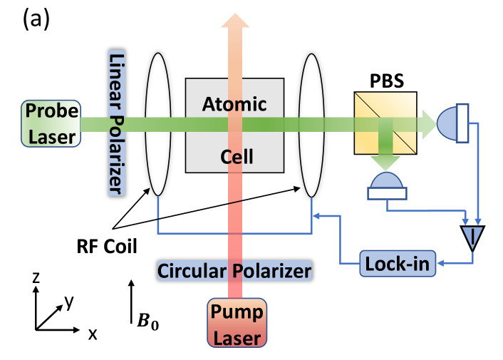
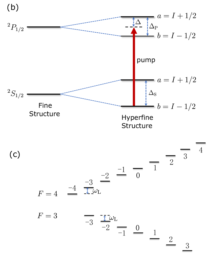
Figure 1: (a) Experimental setup of the alkali-metal-vapor magnetometer. The magnetic field $\vec{B}_{0}$ to be measured is in the $z$-direction, and a pump laser (the red arrow), also propagating in the $z$-direction with circular polarization, is applied to polarize the atomic spins to the $z$-direction. An oscillating magnetic field along the $x$-direction is produced by two RF coils, and the resultant $x$-directional atomic spin polarization is probed by a linearly polarized laser (the green arrow) along the $x$-direction using its optical rotation. Note that the frequency of the probe laser is about $80$ GHz blue detuned from the D2 transition, with the laser power around $10$ mW, so it is a good approximation that the probe laser is not taken into account in the optical pumping process. (b) Schematic of the alkali atoms’ D1 transition in the optical pumping process. Here, $\left.{}^{2}S_{1/2}\right.$ and $\left.{}^{2}P_{1/2}\right.$ represent ground and first excited states, respectively, in the fine structure, and through the hyperfine interaction between the electrons and the nuclei, these levels are further split, with the splitting $\Delta_{\text{S}}$ ($\Delta_{\text{P}}$) for the $\left.{}^{2}S_{1/2}\right.$ ($\left.{}^{2}P_{1/2}\right.$) states. The pump laser (the red arrow) with Rabi frequency $\Omega$ and detuning $\Delta$ (with respect to the frequency difference between the $b=I-1/2$ ground and $a=I+1/2$ excited states) induces transitions between the ground and first excited states. (c) Ground state Zeeman sublevels for cesium ($I=5/2)$, with magnetic numbers marked above/below each level. The energy difference between two adjacent sublevels in the same multiplet is the Larmor frequency $\omega_{\mathrm{L}}$.

For the mechanism of this frequency-dependent light-shift reduction, an intuitive picture is as follows. In the light-narrowing regime with $\Delta=0$, the $b$ ground states are pumped strongly and the alkali atoms mainly populate the $a$ ground state, where most of the magnetic resonance is generated and probed. Considering the Lorentzian form of the AC Stark shift Autler and Townes (1955) for a single state, one might conclude that the dependence of the light shift on the pump beam’s frequency is reduced because of the large hyperfine splitting $\Delta_{\text{S}}$ in the ground state (compared with the line width of the excited states). Note that we do not choose the probe laser’s frequency so that it only measures the magnetic resonance from the $a$ multiplet. Actually, the only function of the probe laser is to measure the response of the atomic spin to the oscillating magnetic field. The fact that the states being pumped differ from the states where most of the spin precession signal is generated arises naturally in the light-narrowing regime with properly tuned pump laser powers.

However, the atomic ground states are incoherently coupled to each other by the light-matter interaction and atomic collisions, so that the light shift cannot be simply written as a Lorentzian or a sum of Lorentzians. Thus we use the master equation to study the light shift in a general alkali-metal-vapor atomic magnetometer, taking into account the light-matter interaction and the relaxation due to collisions between alkali atoms and between alkali atoms and buffer gas Appelt et al. (1998). The interaction between the pump light and the alkali atoms is modeled using the dipole approximation and rotating-wave approximation Walls and Milburn (2008); Gardiner and Zoller (2004). This master equation appeared in some early textbooks and papers Happer (1972); Happer et al. (2010), but it is not easily solved because of its nonlinearity (caused by the mean field approximation for the spin-exchange interaction) and its large superspace Happer (1972); Happer et al. (2010); Gardiner and Zoller (2004). (The full master equation is in a Hilbert space consisting of all the ground and first excited states.) Thus we adiabatically eliminate the excited states in the weak-driving limit, where the Rabi frequency–the coupling strength between the ground and excited states–is much smaller than the excited states’ decay rates, to acquire an effective master equation in a subspace consisting of only the ground states. This can dramatically decrease the calculation power and time needed to solve the nonlinear master equation, and it explicitly shows the intuitive picture of the reduction of the light-shift dependence on the frequency, as well as the light-narrowing effect Appelt et al. (1999). With little cost of calculation, the light shift and line width obtained by solving this effective master equation and using linear response theory Fetter and Walecka (2012) agree well with the experimental data.

The rest of this paper is organized as follows. In section II, we model the system by a full master equation for the density matrix evolution of the alkali atoms, including all the ground states and the first excited states. Starting from this full master equation, in section III, we adiabatically eliminate the excited states in the weak-driving limit and obtain an effective master equation in only the ground-state subspace. It is shown that this effective master equation can give the rate equations Lang et al. (1999) used in many contexts. And when the energy-level broadening of the excited states is much larger than the hyperfine splittings $\Delta_{\text{P}}$ and $\Delta_{\text{S}}$, the light-matter interaction is reduced to a dissipation term that consists of only the electronic spin operators Appelt et al. (1998), leading to the spin temperature distribution. In section IV, we study the linear response of the alkali atoms to the small transverse oscillating magnetic field, both analytically and numerically, showing good agreement between the theoretical predictions and experimental data on both the light shift and line width in a wide frequency regime of the pump laser. Finally, in section V, we summarize our work and show other possible applications of the effective master equation.

II Full master equation description

In this section, we give the full master equation depicting the time evolution of the density matrix $\rho\left(t\right)$ of the alkali atoms. This master equation involves all the energy levels in the ground state and the first excited states Happer (1972); Happer et al. (2010), which can be written as a sum of four Lindblad operators,

$$\partial_{t}\rho=\sum_{n=1}^{4}\mathcal{L}^{\left(n\right)}\rho,$$ (1)

each coming from a different interaction. The first Lindblad term describes the light-matter interaction. Without lost of generality, we assume the pump laser is propagating parallel to the magnetic field’s direction, which defines the magnetic numbers of the hyperfine states, and is left-handed circularly polarized. But this can be easily generalized to the opposite case, i.e., a parallel propagating laser with right-handed circular polarization. This will not change the conclusion of this paper. With the left-handed circularly polarized pump laser, the light-matter interaction contributes to the master equation as

$$\mathcal{L}^{\left(1\right)}\rho = -i\left[H_{\text{lm}},\rho\right]+$$ (2)

$$\Gamma_{\text{sd}}\sum_{l=0,\pm 1}\left(\left|s\right\rangle\left\langle p_{l}\right|\rho\left|p_{l}\right\rangle\left\langle s\right|-\frac{1}{2}\left\{\rho,\left|p_{l}\right\rangle\left\langle p_{l}\right|\right\}\right),$$

where $\Gamma_{\text{sd}}$ is the spontaneous decay rate resulting from the interaction between the alkali atoms and light in the free space; $\left|s\right\rangle$ and $\left|p_{l}\right\rangle$ are the electron’s orbital states $1s$ and $2p$, respectively; and $l$ in $\left|p_{l}\right\rangle$ is its quantum magnetic number. The Hamiltonian $H_{\text{lm}}$ depicting the coupling between the pump beam and the alkali atoms is written in the rotating frame with respect to the laser’s frequency as

$$H_{\text{lm}}=\Omega^{\prime}\left(\left|s\right\rangle\left\langle p_{1}\right|+\left|p_{1}\right\rangle\left\langle s\right|\right),$$ (3)

where $\Omega^{\prime}$ is the Rabi frequency, and the dipole and rotating-wave approximations Walls and Milburn (2008); Gardiner and Zoller (2004) are used. The radiation trapping Molisch and Oehry (1998) effect is not included, since the quenching Seltzer (2008) gas can largely remove it.

The second Lindblad operator depicts the alkali atoms’ energy levels and their Zeeman splitting due to the static magnetic field $\vec{B}_{0}=B_{z}\hat{e}_{z}$:

$$\mathcal{L}^{\left(2\right)}\rho=-i\left[H_{\text{hf}}+H_{\text{Zee}},\rho\right],$$ (4)

where

$$H_{\text{hf}} = \sum_{M}\Delta_{\text{s}}\left|s_{\text{a}}M\right\rangle\left\langle s_{\text{a}}M\right|-\Delta_{\text{p}}\left|p_{\text{b}}M\right\rangle\left\langle p_{\text{b}}M\right|$$ (5)

$$+\Delta\sum_{\text{F=a,b}}\left|p_{\text{F}}M\right\rangle\left\langle p_{\text{F}}M\right|$$

gives the hyperfine structures and

$$H_{\text{Zee}}=\sum_{\text{F=a,b}}\sum_{M}M\omega_{{}_{\text{F}}}\left|s_{\text{F}}M\right\rangle\left\langle s_{\text{F}}M\right|$$ (6)

gives the Zeeman splitting. Here, $\left|s_{\text{F}}/p_{\text{F}}M\right\rangle$ is the hyperfine state in the $1s$ ($\left|s_{\text{F}}M\right\rangle$) or $1p$ ($\left|p_{\text{F}}M\right\rangle$, whose energies have been shifted with respect to the pump beam’s frequency) orbital, with the total angular momentum $F=a$, $b$ and its projection in the $z$-direction $M$. In $H_{\text{Zee}}$,$\ \omega_{{}_{\mathrm{a}}}=-\omega_{{}_{\mathrm{b}}}=\gamma_{\mathrm{e}}B_{z}/(2I+1)\equiv\omega_{{}_{\mathrm{L}}}$ is the Larmor frequency of the atom, where $\gamma_{\mathrm{e}}$ is the gyromagnetic ratio of the electron. Note that only the linear Zeeman splitting in the ground states has been considered, since other interactions with the magnetic field, such as the nonlinear Zeeman interaction for $B_{z}=0.1G$ and the Zeeman splitting in the excited states, are too small to affect the result.

Since there are many alkali atoms and there is much buffer gas (nitrogen in the experiment) in the heated atomic cell, collisions between atoms must be taken into account, resulting in dissipation in the master equation as

$$\mathcal{L}^{\left(3\right)}\rho = \gamma\left(\boldsymbol{S}\cdot\rho\boldsymbol{S-}\frac{1}{2}\left\{\rho,\boldsymbol{S}\cdot\boldsymbol{S}\right\}\right)$$ (7)

$$+\frac{1}{2}\gamma_{\text{se}}\left\langle S_{z}\right\rangle\left(S_{+}\rho S_{-}-S_{-}\rho S_{+}\boldsymbol{+}\left\{\rho,S_{z}\right\}\right)$$

$$+\frac{1}{2}\gamma_{\text{se}}\left\langle S_{+}\right\rangle\left(S_{-}\rho S_{z}-S_{z}\rho S_{-}\boldsymbol{+}\frac{1}{2}\left\{\rho,S_{-}\right\}\right)+\text{H.c.}$$

$$+\Gamma_{\text{pb}}\sum_{m=0,\pm 1}A_{m}\rho A_{j}^{\dagger}-\frac{1}{2}\left\{\rho,A_{m}^{\dagger}A_{m}\right\},$$

where $\boldsymbol{S}$ is the electronic spin operator in the ground state, $S_{\pm}=S_{x}\pm iS_{y}$ is the spin raising/lowering operator, $\gamma_{\text{se}}$ is the spin exchange rate coming from collisions between alkali atoms, and $\gamma=\gamma_{\text{se}}+\gamma_{\text{sd}}$ is the total relaxation rate with the spin destruction rate $\gamma_{\text{sd}}$ coming from collisions between alkali atoms and nitrogen molecules. In addition to spin relaxation, the collisions also cause line broadening of the excited states, with $\Gamma_{\text{pb}}$ being the pressure broadening of the ${}^{2}P_{1/2}$ states due to collisions of the alkali atoms with the nitrogen molecules. During such a collision, the alkali atom in excited states decays to the ground states by transferring its momentum to the nitrogen molecule’s angular momentum, rather than emitting photons. In $\mathcal{L}^{\left(3\right)}$, the jump operators $A_{m}$ are defined as

$$A_{0}=\sum_{m=\pm 1/2}\left|{}^{2}S_{1/2},m\right\rangle\left\langle{}^{2}P_{1/2},m\right|,$$ (8)

$$A_{\pm 1}=\left|{}^{2}S_{1/2},\mp\frac{1}{2}\right\rangle\left\langle{}^{2}P_{1/2},\pm\frac{1}{2}\right|.$$ (9)

It can be shown straightforwardly from $\mathcal{L}^{\left(3\right)}\rho$ that the spin exchange interaction does not change the mean values of the spins, i.e., $\partial_{t}^{\left(3\right)}\left\langle\boldsymbol{S}\right\rangle=0$ if we set $\gamma_{\text{sd}}=0$ and $\Gamma_{\text{pb}}=0$, while the spin destruction interaction exponentially decreases the spin’s mean values, i.e., $\partial_{t}^{\left(3\right)}\left\langle\boldsymbol{S}\right\rangle=-\gamma_{\text{sd}}\left\langle\boldsymbol{S}\right\rangle$ if we set $\gamma_{\text{se}}=0$ and $\Gamma_{\text{pb}}=0$. Here, the time derivative $\partial_{t}^{\left(3\right)}$ means we consider only $\mathcal{L}^{\left(3\right)}\rho$ in the time evolution of the density matrix: $\partial_{t}^{\left(3\right)}\rho=\mathcal{L}^{\left(3\right)}\rho$.

To measure the precession frequency, a small oscillating magnetic field $B_{x}\hat{e}_{x}\cos\omega t$ along the $x$-direction, with amplitude $B_{x}$ and frequency $\omega$, is applied, leading to a time-dependent term in the master equation,

$$\mathcal{L}^{\left(4\right)}\rho=-i\gamma_{\mathrm{e}}B_{x}\cos\omega t\left[S_{x},\rho\right].$$ (10)

Note that the dimension of the superspace Happer (1972); Happer et al. (2010); Gardiner and Zoller (2004) of the full master equation is $4\left(4I+2\right)^{2}$, i.e., there are $4\left(4I+2\right)^{2}$ coupled nonlinear equations to be solved, hence the numerical simulation consumes much time and power. In any case, the physics cannot be revealed in such a big set of nonlinear equations. Therefore, we will simplify this master equation by adiabatically eliminating the excited states.

III Effective master equation in the ground-state subspace

To gain physical insights and accelerate the calculations, we will adiabatically eliminate the excited states in the weak-driving limit in the master equation, where the coupling strength between the ground and excited states is much smaller than the energy-level broadening of the corresponding excited state, i.e., $\Omega\equiv\sqrt{2/3}\Omega^{\prime}\ll\Gamma_{\text{sd}}/2+\Gamma_{\text{pb}}$, which has been shown in many experiments. Furthermore, when $\gamma_{\mathrm{e}}B_{x}\ll\gamma$, we can apply linear response theory Fetter and Walecka (2012) and consider the effect of the transverse field at the very end. Therefore, in this case we will drop the Lindblad term $\mathcal{L}^{\left(4\right)}\rho$ in the master equation.

Adiabatic elimination in the master equation is common in quantum optics when working with open systems Gardiner and Zoller (2004); Wallquist et al. (2010); Schwager et al. (2013). There are several ways to accomplish adiabatic elimination. For example, one can utilize a generating function, as is commonly done in the Fröhlich transformation Cohen-Tannoudji et al. (2006), but in the superspace, adiabatic elimination is usually performed in the motion equations Gardiner and Zoller (2004); Wallquist et al. (2010); Schwager et al. (2013). Here, we apply the latter to the alkali-metal-vapor atomic systems. Following the standard procedure, we first define two projection operators $\mathcal{P}$ and $\mathcal{Q}=1-\mathcal{P}$, where $\mathcal{P}$ projects any given operators in the Hilbert space or vectors in the superspace to the ground-state subspace. For instance, when performing in the density matrix, $\mathcal{P}\rho$ gives

$$\mathcal{P}\rho=\sum_{FMF^{\prime}M^{\prime}}\left\langle s_{F}M\right|\rho\left|s_{F^{\prime}}M^{\prime}\right\rangle\left|s_{F}M\right\rangle\left\langle s_{F^{\prime}}M^{\prime}\right|.$$ (11)

Next, we write the full master equation (1) in the $\mathcal{P}$- and $\mathcal{Q}$-spaces and adiabatically eliminate the $\mathcal{Q}$-space, acquiring an effective master equation in the $\mathcal{P}$-space. For this purpose, we separate the Lindblad operators in the full master equation (1) into two parts,

$$\partial_{t}\rho=\left(\mathcal{L}_{0}+\mathcal{L}_{1}\right)\rho,$$ (12)

where

$$\mathcal{L}_{1}\rho\equiv-i\left[H_{\text{lm}},\rho\right]$$ (13)

is the perturbation that couples the $\mathcal{P}$-space to the $\mathcal{Q}$-space  and $\mathcal{L}_{0}\rho=\left(\sum_{n=1}^{3}\mathcal{L}^{\left(n\right)}-\mathcal{L}_{1}\right)\rho$ is the zeroth order term. Noting that $\mathcal{P}+\mathcal{Q}=1$, $\mathcal{Q}$$\mathcal{L}_{0}\mathcal{P}=0$, and $\mathcal{PL}_{0}\mathcal{P}=0$, we can write the density matrix’s evolution in the $\mathcal{P}$- and $\mathcal{Q}$-spaces respectively as

$$\partial_{t}\mathcal{P}\rho=\mathcal{PL}_{0}\mathcal{P}\rho+\mathcal{PL}_{0}\mathcal{Q}\rho+\mathcal{PL}_{1}\mathcal{Q}\rho,$$ (14)

$$\partial_{t}\mathcal{Q}\rho=\mathcal{Q}\text{{}}\mathcal{L}_{0}\mathcal{Q}\rho+\mathcal{Q}\text{{}}\mathcal{L}_{1}\mathcal{P}\rho+\mathcal{Q}\text{{}}\mathcal{L}_{1}\mathcal{Q}\rho.$$ (15)

To adiabatically eliminate the $\mathcal{Q}$-space, we solve $\mathcal{Q}\rho$ from Eq. (15) and substitute it in Eq. (14). The solution for $\mathcal{Q}\rho$ in Eq. (15) is

$$\mathcal{Q}\rho\left(t\right)=\int_{0}^{t}e^{\mathcal{Q}\left(\mathcal{L}_{0}+\mathcal{L}_{1}\right)\left(t-t^{\prime}\right)}\mathcal{Q}\text{{}}\mathcal{L}_{1}\mathcal{P}\rho\left(t^{\prime}\right)dt^{\prime},$$ (16)

where we assume an initial condition $\mathcal{Q}\rho\left(0\right)=0$. This assumption shows that the system is initially in the $\mathcal{P}$-space, which is reasonable, since before the interaction with the pump laser, the steady state of the system is in the $\mathcal{P}$-space. Then, substituting this solution of $\mathcal{Q}\rho\left(t\right)$ in Eq. (14), for the second order of $\mathcal{L}_{1}$, we acquire the density matrix in the ground-state subspace,

$$\partial_{t}\mathcal{P}\rho\left(t\right) \approx \mathcal{PL}_{0}\mathcal{P}\rho\left(t\right)+\mathcal{PL}_{1}\int_{0}^{t}e^{\mathcal{Q}\text{ }\mathcal{L}_{0}\left(t-t^{\prime}\right)}\mathcal{Q}\text{{}}\mathcal{L}_{1}\mathcal{P}\rho\left(t\right)dt^{\prime}$$ (17)

$$+\mathcal{PL}_{0}\int_{0}^{t}e^{\mathcal{Q}\text{{}}\mathcal{L}_{0}\left(t-t^{\prime}\right)}(1+$$

$$\int_{0}^{t-t^{\prime}}dt^{\prime\prime}e^{-\mathcal{Q}\text{{}}\mathcal{L}_{0}t^{\prime\prime}}\mathcal{Q}\text{{}}\mathcal{L}_{1}e^{\mathcal{Q}\text{{}}\mathcal{L}_{0}t^{\prime\prime}})\mathcal{Q}\text{{}}\mathcal{L}_{1}\mathcal{P}\rho\left(t\right)dt^{\prime},$$

where we have applied the Born-Markov approximation Walls and Milburn (2008); Gardiner and Zoller (2004) to replace $\rho\left(t^{\prime}\right)$ by $\rho\left(t\right)$ in the integral and extend the upper limit $t$ in the integration to $+\infty$. The Born-Markov approximation has been verified in many quantum open systems Gardiner and Zoller (2004); Walls and Milburn (2008), given that the exponent $e^{\mathcal{L}_{0}t}$ decays on a time scale much smaller than that of $\mathcal{P}\rho\left(t\right)$, which is the case in our system.

After straightforward calculations using the concrete expressions of $\mathcal{L}_{0}$ and $\mathcal{L}_{1}$, the effective master equation in the ground-state subspace is

$$\partial_{t}\rho_{g} = -i\left[H_{\text{hf}}+H_{\text{Zee}},\rho_{g}\right]+\gamma\left(\boldsymbol{S}\cdot\rho_{g}\boldsymbol{S-}\frac{1}{2}\left\{\rho_{g},\boldsymbol{S}\cdot\boldsymbol{S}\right\}\right)$$ (18)

$$+\frac{1}{2}\gamma_{\text{se}}\left\langle S_{z}\right\rangle\left(S_{+}\rho_{g}S_{-}-S_{-}\rho_{g}S_{+}\boldsymbol{+}\left\{\rho_{g},S_{z}\right\}\right)+\frac{1}{2}\gamma_{\text{se}}\left\langle S_{+}\right\rangle\left(S_{-}\rho_{g}S_{z}-S_{z}\rho_{g}S_{-}\boldsymbol{+}\frac{1}{2}\left\{\rho_{g},S_{-}\right\}\right)+\text{H.c.}$$

$$+\sum_{n=1}^{3}\sum_{FMF\prime M^{\prime}}\left[\Gamma_{FMF\prime M^{\prime}}^{(n)}J_{FF\prime M}^{\left(n\right)}\rho_{g}J_{FF\prime M^{\prime}}^{\left(n\right)\dagger}\right]-\sum_{FMM^{\prime}}\left(\Gamma_{FM}+\Gamma_{FM^{\prime}}^{\ast}\right)J_{FM}\rho_{g}J_{FM^{\prime}}$$

where $\ \rho_{g}=\mathcal{P}\rho\left(t\right)$ is the density matrix in the ground-state subspace, the jump operators $J_{FF\prime M}^{\left(n\right)}$ are

$$J_{FF\prime M}^{\left(1\right)}=\left|F^{\prime},M+1\right\rangle\left\langle FM\right|,$$ (19)

$$J_{FF\prime M}^{\left(2\right)}=\left|F^{\prime}M\right\rangle\left\langle FM\right|,$$ (20)

$$J_{FF\prime M}^{\left(3\right)}=\left|F^{\prime},M+2\right\rangle\left\langle FM\right|,$$ (21)

the operator $J_{FM}$ is

$$J_{FM}=\left|FM\right\rangle\left\langle FM\right|,$$ (22)

and the pump-laser-induced relaxation rates are

$$\Gamma_{FMF\prime M^{\prime}}^{(1)}=\frac{\Gamma_{\text{pb}}\Omega^{2}}{\left|\tilde{\Delta}_{FF^{\prime}}\right|^{2}}g_{2;FMFM^{\prime}}g_{1;F^{\prime}M+1,F^{\prime}M^{\prime}+1},$$ (23)

$$\Gamma_{FMF\prime M^{\prime}}^{(2)}=g_{2;FMFM^{\prime}}g_{2;F^{\prime}MF^{\prime}M^{\prime}}\sum_{F_{1}F_{2}}\frac{\Omega^{2}\Gamma_{\text{pb}}}{\tilde{\Delta}_{FF_{1}}\tilde{\Delta}_{FF_{2}}^{\ast}}g_{1;F_{1}M+1,F_{2}M^{\prime}+1}^{2},$$ (24)

$$\Gamma_{FMF\prime M^{\prime}}^{(3)}=g_{2;FMFM^{\prime}}g_{1;F^{\prime}M+2,F^{\prime}M^{\prime}+2}\sum_{F_{1}F_{2}}\frac{\Omega^{2}\Gamma_{\text{pb}}}{\tilde{\Delta}_{FF_{1}}\tilde{\Delta}_{FF_{2}}^{\ast}}g_{1;F_{1}M+1,F_{2}M^{\prime}+1}g_{2;F_{1}M+1,F_{2}M^{\prime}+1},$$ (25)

$$\Gamma_{FM}^{(4)}=\sum_{F^{\prime}}\frac{\Omega^{2}}{\tilde{\Delta}_{FF^{\prime}}}g_{2;FMFM}g_{1;F^{\prime}M+1,F^{\prime}M+1},$$ (26)

with the coefficients

$$g_{n,FMF\prime M^{\prime}}=CG_{F}\left(n,M\right)CG_{F^{\prime}}\left(n,M^{\prime}\right)$$ (27)

and

$$\tilde{\Delta}_{FF^{\prime}}=\Delta_{FF^{\prime}}-i\Gamma_{\text{pb}}.$$ (28)

Here, $CG_{F}\left(n,M\right),$ $n=1$, $2$, are the Clebsch-Gordan coefficients, defined as

$$CG_{F}\left(n,M\right)=\left\langle\left.I,M-\frac{\left(-\right)^{n-1}}{2};\frac{1}{2},\frac{\left(-\right)^{n-1}}{2}\right|FM\right\rangle,$$ (29)

and $\Delta_{\text{aa}}=\Delta-\Delta_{\text{s}}$, $\Delta_{\text{ab}}=\Delta-\Delta_{\text{s}}-\Delta_{\text{p}}$, $\Delta_{\text{ba}}=\Delta$, and $\Delta_{\text{bb}}=\Delta-\Delta_{\text{p}}$ are the energy differences. These energy differences $\Delta_{FF^{\prime}}$ are the detunings between the pump laser’s frequency and the transition frequency between the ground state in the $F$ multiplet and the excited state in the $F^{\prime}$ multiplet. We also define the corresponding effective detunings $\tilde{\Delta}_{FF^{\prime}}$, given that each excited state “gains” an imaginary energy $-i\Gamma_{\text{pb}}$ representing its energy level broadening. Note that we simplify the derivation of Eq. (18) by assuming the hyperfine splitting $\Delta_{\text{s}}$ is much larger than the (effective) decay rates, which is the case for most alkali-vapor atomic magnetometers, such that the coherence between the $a$ and $b$ multiplets, as well as the contribution to the effective detuning $\tilde{\Delta}_{FF^{\prime}}$ from the electronic spin relaxation and the Zeeman splitting, can be neglected. Moreover, we assume that the spontaneous decay rate is much smaller than the pressure broadening, $\Gamma_{\text{sd}}/2\ll\Gamma\equiv\Gamma_{\text{pb}}$, which occurs in atomic vapors with high pressure buffer gas. Thus the spontaneous decay term can be neglected in the master equation. When the condition $\Gamma_{\text{sd}}/2\ll\Gamma_{\text{pb}}$ is not met, we can obtain a similar effective master equation in which the effective decay rates $\Gamma_{FMF\prime M^{\prime}}^{(j=1,2,3)}$ and $\Gamma_{FM}^{4}$ are slightly different.

The effective master equation (18) is valid in an extensive parameter regime. In particular, when the energy splittings $\Delta_{\text{s}}$ and $\Delta_{\text{p}}\$are both much smaller than the excited states’ energy broadening $\Gamma$, the master equation can be written in the compact form Appelt et al. (1998)

$$\partial_{t}\rho_{g} = \left(\mathcal{L}^{\left(2\right)}+\mathcal{L}^{\left(3\right)}\right)\rho_{g}$$ (30)

$$+\Gamma_{\mathrm{OP}}\left[S_{+}\rho_{g}S_{-}+S_{z}\rho_{g}S_{z}+\frac{1}{2}\left\{S_{z},\rho_{g}\right\}-\frac{3}{4}\rho_{g}\right]$$

$$-i\Delta_{\mathrm{LS}}\left[S_{z},\rho_{g}\right],$$

where

$$\Gamma_{\mathrm{OP}}=\frac{\eta^{2}\Gamma}{\Gamma^{2}+\Delta^{2}}$$ (31)

is the optical pumping rate and

$$\Delta_{\mathrm{LS}}=\frac{-\eta^{2}\Delta}{\Gamma^{2}+\Delta^{2}}$$ (32)

is the light shift. This master equation (30) gives the Bloch equations and the spin temperature distribution Walker and Happer (1997); Appelt et al. (1998), where populations in states with the same magnetic number $M$ are the same.

In an extensive parameter regime, including when the condition $\Delta_{\text{s,p}}\ll\Gamma_{\text{pb}}$ is not met, one can use the general master equation (18) we have derived. It can be shown in (18) that when the coherence between the two multiplets $a\$and $b$ in the spin relaxation term are ignored, the diagonal elements of the density matrix $\rho_{g}$ are decoupled from the diagonal ones. As a result, we obtain the rate equations Lang et al. (1999), i.e., the evolution of the diagonal elements of the density matrix. In this case, only the diagonal terms are non-vanishing in the steady-state solution to the master equation, i.e., the polarization is along the $z$-direction and the mean values $\left\langle S_{\pm}\right\rangle$ in $\mathcal{L}^{\left(3\right)}$ are zero. This reduces the number of coupled nonlinear equations from $4\left(4I+2\right)^{2}$ to $4I+2$, and speeds up the numerical calculation.

In the experiment Guo et al. (2019) with cesium atoms, whose nuclear spin is $7/2$ and energy splittings are $\Delta_{\text{S}}=9.193$ GHz and $\Delta_{\text{P}}=1.168$ GHz, the atomic cell is cubic, with inner size $4\times 4\times 4\mathrm{mm}^{3}$, and is heated to $90$ Celsius. The power of the pump beam is 700 $\mu$W, with right-handed circular polarization. The magnetic field $B_{0}=0.1$G along the $z$-direction. Thus the atoms are mostly pumped to states with negative magnetic numbers, and the polarization is negative. This is equivalent to a left-handed circularly polarized pump laser propagating antiparallel to the direction of the magnetic field. In this case, we only need to change $B_{0}$ to $-B_{0}$ in the effective master equation (18), while keeping the definition of the $z$-direction that defines the magnetic states. With the Rabi frequency $\Omega=4.1$ MHz, spin exchange rate $\gamma_{\text{se}}=1.31$ KHz, total spin relaxation rate $\gamma=1.53$ KHz, and excited states’ energy broadening $\Gamma=0.6$ GHz for the 100 torr nitrogen case, while $\gamma=1.65$vKHz, $\Gamma=4.2$ GHz for the 700 torr nitrogen case, we numerically solve the master equation (18) for $\rho_{g}$ in the long term limit.

With the steady-state solution $\rho_{g}^{\left(0\right)}$, where $\rho_{g}^{\left(0\right)}$ satisfies the effective master equation (18) and$\ \partial_{t}\rho_{g}^{\left(0\right)}=0$, the electronic spin polarization $\left\langle S_{z}\right\rangle$ as a function of the detuning $\Delta$ is plotted in Fig. 2. For the 100 torr nitrogen case, two peaks, corresponding to $\Delta\approx 0$ (marked by circle (a)) and $\Delta_{aa}\approx 0$ (marked by circle (c)), are shown in the polarization curve, corresponding to two pump frequencies resonant with the transition frequencies between the $a$/$b$ mutiplets and the excited states. However, for the 700 torr nitrogen case, these two peaks (marked by circles (b) and (d)) cannot be distinguished because of the large energy level broadening $\Gamma$ of the excited states. Comparing the polarizations at these four circles in Fig. 2, we see that the polarization in (a) is larger than in (b), while the polarization in (c) is smaller than in (d). This is because the effective optical pumping rates $\Gamma_{FMF\prime M^{\prime}}^{(j=1,3)}$ are inversely proportional to $\Gamma$. (We note that the optical pumping process is generally complicated, as shown in Eq. (18), and there does not exist a simple optical pumping rate, as shown in Eq. (31).) In (a) and (b), $\Delta=0$ and the ground state with $F=3$ are more efficiently pumped and depleted, leaving the atoms mostly in the $F=4$ states, which contribute more to the electrons’ polarization. Thus the larger the energy level broadening $\Gamma$ the smaller the polarization. However, in (c) and (d), $\Delta_{aa}=0$ and the $F=4$ ground states are more efficiently pumped, leaving the atoms populating the $F=4$ states less than in cases (a) and (b). Therefore, the larger $\Gamma$ causes more polarization. To verify this, we plotted the ground state populations, i.e., the diagonal terms of the density matrix in Fig. 3, for the four resonant cases (a)-(d) marked in Fig. 2. Fig. 3 shows that the populations in the $F=4$ ground states are larger in (a) and (d), compared with those in (b) and (c), respectively. Moreover, in each case, the populations in states $\left|4,m\right\rangle$ and$\ \left|3,m\right\rangle$ are different, especially when $m=3$, which is shown explicitly in the figures. Thus the spin temperature distribution Walker and Happer (1997); Appelt et al. (1998) is not valid.

Figure 2: Electron polarizations for cesium atoms in the steady-state solution to the effective master equation in the ground state subspace, as functions of the pump beam’s detuning $\Delta$. For a smaller decay rate (100 torr, blue line) of the excited state such that $\Gamma\ll\Delta_{\text{S}}$, there are two peaks in the electron’s polarization, around two resonant frequencies $\Delta=0$ (point (a)) and $\Delta_{\text{aa}}=0$ (point (c)). In the 700 torr case (red line), the decay rate $\Gamma$ is comparable to $\Delta_{\text{S}}$. Therefore, the two polarization peaks around the two frequencies ((b) and (d)) cannot be distinguished. The populations in the ground states at these four points (a)-(d) are plotted in Fig. 3.

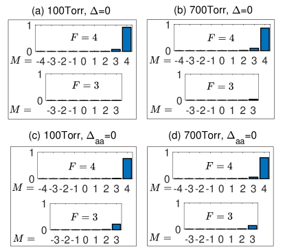
Figure 3: Population distribution in the hyperfine states at two resonant frequencies $\Delta=0$ ((a) and (b)) and $\Delta_{\text{aa}}=0$ ((c) and (d)), for different energy level broadening $\Gamma$ of the excited state, corresponding to the four points in Fig. 2. When the lower ground states with $F=3$ are pumped ($\Delta=0$), the smaller the decay rate $\Gamma$ the smaller the population in the $F=3$ states. However, when the upper states with $F=4$ are pumped ($\Delta_{\text{aa}}=0$), a smaller $\Gamma$ gives a larger population in the $F=3$ states. Note that the populations in states $\left|4,m\right\rangle$ and$\ \left|3,m\right\rangle$ are different, especially when $m=3$. Thus the spin temperature distribution is not valid.

Having solved the steady-state solution $\rho_{g}^{\left(0\right)}$, we will study the light shift and line width acquired from the linear response Fetter and Walecka (2012) of the atoms to an oscillating transverse magnetic field.

IV Frequency-dependent light-shift reduction and light narrowing

In the presence of the oscillating magnetic field $B_{x}\hat{e}_{x}\cos\omega t$ in the $x$-direction, where $\gamma_{\mathrm{e}}B_{\mathrm{x}}$ ($B_{\mathrm{x}}=3$nT in the experiment) is much smaller than the decay rate $\gamma$ or $\Gamma_{FMF\prime M^{\prime}}^{(n)}$, the master equation can be written as

$$\partial_{t}\rho_{g}=\mathcal{\bar{L}}_{0}\rho_{g}+\mathcal{\bar{L}}_{1}\rho_{g}\text{,}$$ (33)

where

$$\mathcal{\bar{L}}_{0}\rho_{g} = -i\left[H_{\text{hf}}+H_{\text{Zee}},\rho_{g}\right]$$ (34)

$$+\gamma\left(\boldsymbol{S}\cdot\rho_{g}\boldsymbol{S-}\frac{1}{2}\left\{\rho_{g},\boldsymbol{S}\cdot\boldsymbol{S}\right\}\right)$$

$$+\frac{1}{2}\gamma_{\text{se}}\left\langle S_{z}\right\rangle\left(S_{+}\rho_{g}S_{-}-S_{-}\rho_{g}S_{+}\boldsymbol{+}\left\{\rho_{g},S_{z}\right\}\right)$$

$$+\sum_{n=1}^{3}\sum_{FMF\prime M^{\prime}}\left[\Gamma_{FMF\prime M^{\prime}}^{(n)}J_{FF\prime M}^{\left(n\right)}\rho_{g}J_{FF\prime M^{\prime}}^{\left(n\right)\dagger}\right]$$

$$-\sum_{FMM^{\prime}}\left(\Gamma_{FM}+\Gamma_{FM^{\prime}}^{\ast}\right)J_{FM}\rho_{g}J_{FM^{\prime}}$$

is the zero-order term, and

$$\mathcal{\bar{L}}_{1}\rho_{g} = \frac{1}{2}\gamma_{\text{se}}\left\langle S_{+}\right\rangle\left(S_{-}\rho_{g}S_{z}-S_{z}\rho_{g}S_{-}\boldsymbol{+}\frac{1}{2}\left\{\rho_{g},S_{-}\right\}\right)$$ (35)

$$+\text{H.c.}+\mathcal{L}^{\left(4\right)}\rho_{g}$$

is the first-order perturbation. Here, the zero-order Lindblad operator $\mathcal{\bar{L}}_{0}$ is different from the right side of Eq. (18) regarding the terms containing $\left\langle S_{\pm}\right\rangle$, since $\left\langle S_{\pm}\right\rangle$ is zero from the zero-order solution $\rho_{g}^{\left(0\right)}$. That is, the polarization in directions other than the $z$-direction is induced by the magnetic field $B_{x}\hat{e}_{x}\cos\omega t$. As a result, the terms with $\left\langle S_{\pm}\right\rangle$ are perturbations and it is in $\mathcal{\bar{L}}_{1}$ rather than in $\mathcal{\bar{L}}_{0}$.

To the first order of $\mathcal{\bar{L}}_{1}$, $\rho_{g}$ in the long-term limit has three parts:

$$\rho_{g}=\rho_{g}^{\left(0\right)}+\rho_{g}^{\left(+\right)}e^{i\omega t}+\rho_{g}^{\left(-\right)}e^{-i\omega t},$$ (36)

where $\rho_{g}^{\left(0\right)}$ was obtained above by solving the equation $\mathcal{\bar{L}}_{0}\rho_{g}^{\left(0\right)}=0$; $\rho_{g}^{\left(+\right)}$ is the positive-frequency part of $\rho_{g}$ that fulfills

$$\left(\mathcal{\bar{L}}_{0}-i\omega\right)\rho_{g}^{\left(+\right)}+\mathcal{\bar{L}}_{1}^{\left(+\right)}\rho_{g}^{\left(0\right)}=0,$$ (37)

with its positive-frequency Lindblad operator $\mathcal{\bar{L}}_{1}^{\left(+\right)}$ defined as

$$\mathcal{\bar{L}}_{1}^{\left(+\right)}\rho_{g}^{\left(0\right)} = -\frac{i}{2}\gamma_{\mathrm{e}}B_{x}\left[S_{x},\rho_{g}^{\left(0\right)}\right]+\frac{1}{2}\gamma_{\text{se}}\text{Tr}\left[S_{+}\rho_{g}^{\left(+\right)}\right]$$ (38)

$$\times\left(S_{-}\rho_{g}^{\left(0\right)}S_{z}-S_{z}\rho_{g}^{\left(0\right)}S_{-}\boldsymbol{+}\frac{1}{2}\left\{\rho_{g}^{\left(0\right)},S_{-}\right\}\right)$$

$$+\text{H.c.;}$$

and the negative-frequency part $\rho_{g}^{\left(-\right)}=\rho_{g}^{\left(+\right)\dagger}$ to ensure the Hermitian of the density matrix $\rho_{g}$. Note that $\mathcal{\bar{L}}_{1}^{\left(+\right)}$ is dependent on $\rho_{g}^{\left(+\right)}$ through the mean value $\left\langle S_{+}\right\rangle$. Therefore, $\mathcal{\bar{L}}_{1}^{\left(+\right)}\rho_{g}^{\left(0\right)}$ can be decomposed to two parts: $\mathcal{\bar{L}}_{1}^{\left(+\right)}\rho_{g}^{\left(0\right)}=\mathcal{\bar{L}}_{0}^{\left(+\right)}\rho_{g}^{\left(+\right)}+\mathcal{\bar{L}}_{1}^{\prime\left(+\right)}\rho_{g}^{\left(0\right)}$, where

$$\mathcal{\bar{L}}_{1}^{\prime\left(+\right)}\rho_{g}^{\left(0\right)}=-\frac{i}{2}\gamma_{\mathrm{e}}B_{x}\left[S_{x},\rho_{g}^{\left(0\right)}\right],$$

and $\mathcal{\bar{L}}_{0}^{\left(+\right)}$ contains $\rho_{g}^{\left(0\right)}$ but not $\rho_{g}^{\left(+\right)}$. As a result, the solution of $\rho_{g}^{\left(+\right)}$ is

$$\rho_{g}^{\left(+\right)}=-\left(\mathcal{\bar{L}}_{0}+\mathcal{\bar{L}}_{0}^{\left(+\right)}-i\omega\right)^{-1}\mathcal{\bar{L}}_{1}^{\prime\left(+\right)}\rho_{g}^{\left(0\right)}.$$ (39)

Consequently, the electrons’ polarization in the $x$-direction can be written as

$$\left\langle S_{x}\left(t\right)\right\rangle=\text{Re}\left\langle S_{x}^{+}\right\rangle\cos\omega t-\text{Im}\left\langle S_{x}^{+}\right\rangle\sin\omega t,$$ (40)

where $\left\langle S_{x}^{+}\right\rangle=2$Tr$\left[S_{x}\rho_{g}^{\left(+\right)}\right]$. Here, $\left\langle S_{x}^{+}\right\rangle$ is a function of $\omega$. In the experiment, the measured Larmor frequency $\omega_{\mathrm{L}}$ is determined by the zero-crossing $\omega_{\mathrm{0}}$ of Re$\left\langle S_{x}^{+}\right\rangle$, and the line width $w$ is defined as half the difference between frequencies corresponding to the maximum and minimum  of Re$\left\langle S_{x}^{+}\right\rangle$.

As shown in Sec. III, there are only diagonal terms in the steady-state $\rho_{g}^{\left(0\right)}$. Thus, in the superspace Happer (1972); Happer et al. (2010); Gardiner and Zoller (2004), $\mathcal{\bar{L}}_{1}^{\prime\left(+\right)}\rho_{g}^{\left(0\right)}$ is a column vector in the subspace $\left\{\left|FM\right\rangle\left\langle FM\pm 1\right|\right\}$, and $\mathcal{\bar{L}}_{0}+\mathcal{\bar{L}}_{0}^{\left(+\right)}$ is a matrix that does not couple this subspace $\left\{\left|FM\right\rangle\left\langle FM\pm 1\right|\right\}$ to the others. In general, the zero-crossing $\omega_{\mathrm{0}}$ and the line width $w$ are obtained by diagonalizing the matrix $\mathcal{\bar{L}}_{0}+\mathcal{\bar{L}}_{0}^{\left(+\right)}$, which can only be done numerically. But to acquire an intuitive picture, we can analyze the diagonal terms of $\mathcal{\bar{L}}_{0}+\mathcal{\bar{L}}_{0}^{\left(+\right)}$.

When the Larmor frequency $\omega_{\mathrm{L}}$ is much larger than the dissipation rates that contribute to the real parts of the eigenvalues of $\mathcal{\bar{L}}_{0}+\mathcal{\bar{L}}_{0}^{\left(+\right)}$, the zeros-crossing $\omega_{\mathrm{0}}$ will be around $\pm\omega_{\mathrm{L}}$, the eigenvalues of $i\mathcal{L}^{\left(2\right)}$ in the subspace $\left\{\left|FM\right\rangle\left\langle FM\pm 1\right|\right\}$. Here, we focus on $\omega$ around the positive frequency $\omega_{\mathrm{L}}$, corresponding to the subspace $\left\{\left|aM\right\rangle\left\langle a,M+1\right|,\left|bM\right\rangle\left\langle b,M-1\right|\right\}$ (the coherence between states with different $F$ has been ignored, for the same reason as in Sec. III.). Especially, when the atoms mainly populate the state $\left|aa\right\rangle$, the most weighted diagonal element of $\mathcal{\bar{L}}_{0}+\mathcal{\bar{L}}_{0}^{\left(+\right)}$ is $i\tilde{\omega}-\tilde{\gamma}$ in the basis $\left|a,a-1\right\rangle\left\langle aa\right|$, where the frequency

$$\tilde{\omega}=\omega_{\mathrm{L}}+\frac{1}{2I+1}\frac{\Omega^{2}\Delta_{aa}}{\Gamma^{2}+\Delta_{aa}^{2}}$$ (41)

and the line broadening

$$\tilde{\gamma} = \frac{\Omega^{2}}{2I+1}\frac{\Gamma}{\Gamma^{2}+\Delta_{aa}^{2}}+\frac{I+1}{2I+1}\gamma$$ (42)

$$-\frac{1}{2I+1}\gamma_{ex}-\frac{2I}{2I+1}\gamma_{ex}\left\langle S_{z}\right\rangle.$$

In the light-narrowing regime with $\Delta\approx 0$, $\tilde{\omega}$ can be approximated in the vicinity of this resonant frequency as

$$\tilde{\omega}=\omega_{\mathrm{L}}-\frac{1}{2I+1}\frac{\Omega^{2}\Delta_{\text{s}}}{\Gamma^{2}+\Delta_{\text{s}}^{2}}+\delta\omega,$$ (43)

where

$$\delta\omega=\frac{1}{2I+1}\frac{\Omega^{2}\Delta}{\Gamma^{2}+\Delta_{\text{s}}^{2}}$$ (44)

is the frequency-dependent light shift that leads to measurement inaccuracy if the pump laser’s frequency fluctuates. Because of the large hyperfine splitting $\Delta_{\text{s}}$, the frequency-dependent light shift $\delta\omega$ can be strongly reduced. Futhermore, for fully polarized atoms, i.e., $\left\langle S_{z}\right\rangle=1/2$, the line width

$$\tilde{\gamma}=\frac{\Omega^{2}}{2I+1}\frac{\Gamma}{\Gamma^{2}+\Delta_{aa}^{2}}+\frac{I+1}{2I+1}\gamma_{\text{sd}},$$ (45)

and the spin-exchange relaxation does not contribute to the line width, which makes perfect line narrowing Appelt et al. (1999); Scholtes et al. (2011) possible.

The Lorentzian light shift $\delta\omega$ in Eq. (44) is actually the AC Stark shift. It gives an intuitive picture of why the light shift is reduced in the light-narrowing regime. But, as shown in $\mathcal{\bar{L}}_{0}+\mathcal{\bar{L}}_{0}^{\left(+\right)}$ in Eq. (39), each pair of adjacent magnetic levels has its own precession frequency (the imaginary part of the diagonal terms of $\mathcal{\bar{L}}_{0}+\mathcal{\bar{L}}_{0}^{\left(+\right)}$), and they are all coupled (the non-zero off-diagonal terms of $\mathcal{\bar{L}}_{0}+\mathcal{\bar{L}}_{0}^{\left(+\right)}$). Thus the total light shift is generally not a single Lorentzian or a sum of several Lorentzians. To obtain the exact result, we numerically solve Eq. (39) and search for the zero-crossing $\omega_{\mathrm{0}}$ and the line width $w$. The numerical results, which are shown in Fig. 4, with the same parameters as in Fig. 2, agree well with the experimental data. For the light shift shown in Fig. 4(a), in both the 100 and 700 torr cases, in the vicinity of the frequency $\Delta=\Delta_{\text{S}}$ ($\Delta_{\text{aa}}\approx 0$), where the $F=a$ ground states are pumped, the blue lines have two (100 torr) or one (700 torr) zero-crossings, corresponding to the resonant frequencies, and the light shift changes much while the frequency varies. However, when $\Delta$ is around $0$, i.e., when the $F=b$ ground states are pumped, no zero-crossing appears in the blue lines and the frequency-dependent light shift is highly reduced. The line width shown in 4(b) has a dip around the frequency $\Delta=0$. This is the light-narrowing effect. Note that at a large detuning limit ($-5$ and $15$ GHz, for instance), the light’s effect tends to vanish. As a result, at infinite detunings, the light shift goes to zero and the line width tends to be a constant, independent of the pump beam’s Rabi frequency $\Omega$, its detuning $\Delta$, or the excited states’ decay rate $\Gamma$ Happer and Tam (1977).

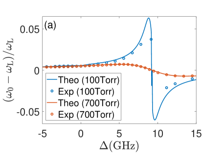
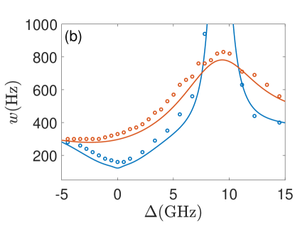
Figure 4: Light shift (a) and line width (b) for the 100 torr and 700 torr nitrogen cases as functions of the pump beam’s detuning $\Delta$ (the legend in (b) is the same as in (a)). The theoretical results are shown by the lines, and the experimental data are shown by circles with corresponding colors (the experimental data have been calibrated so that the light shift at infinite detuning is zero). Both the theoretical and experimental results show that the light shift’s dependence on the pump laser’s frequency is largely reduced around the resonant point $\Delta$, especially compared to the light shift around $\Delta_{\text{aa}}=0$. In this light-shift-reduced regime, the line width is narrowed, as shown in (b).

V Conclusions and outlook

We have studied in detail the mechanism of the light shift and light-narrowing effects in alkali-metal-vapor magnetometers. Starting from the full master equation for the alkali atom’s density matrix, we acquire the effective master equation in the ground-state subspace by adiabatically eliminating the excited states in the weak-driving limit. This effective master equation cannot only save power and time for the numerical calculations, but can reveal the intuitive picture of the frequency-dependent light-shift reduction: in the light-narrowing regime, the $F=b$ ground states are depleted by the pump laser, and the atoms mostly populate the $F=a$ states. As a result, the light shift is reduced since the pump beam’s frequency is largely detuned from the transition frequency between the most populated ground states ($F=a$) and the excited states. We compare the theoretical results to the experimental data, and find they agree for both the light shift and line width.

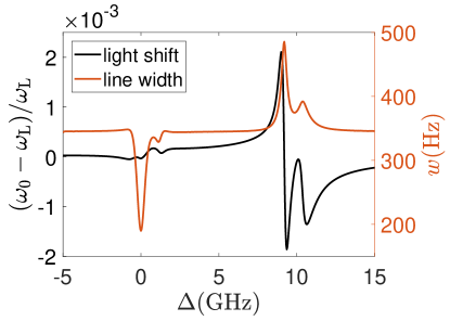
Figure 5: Light shift (black line) and line width (red line) for $\Gamma=0.2$ GHz and $\Omega=0.5$ MHz, with other parameters the same as the 100 torr nitrogen case in the cesium vapor experiment. With smaller $\Gamma$ and $\Omega$, more peaks and zero-crossings are shown in both the light shift and line width.

We note that the effective master equation we have obtained is general and is valid in an extensive parameter regime for alkali-vapor magnetometers. Particularly, it can lead to the spin temperature distribution in the limit that the hyperfine splittings in both the ground and excited states can be ignored when the broadening of the excited states is much larger than them. Since it consumes little time and power to solve this effective master equation, one can use it to quickly explore a large parameter regime to optimize the physical properties. For example, with a smaller decay rate $\Gamma=0.2$ GHz and Rabi frequency $\Omega=0.5$ MHz, while other parameters are the same as in Fig. 2 for the 100 torr nitrogen case, the light shift and line width are acquired and shown in Fig. 5. Here, more peaks and zero-crossings can be distinguished, corresponding to four resonant frequencies $\Delta_{\mathrm{FF^{\prime}}}=0$ with $F$, $F^{\prime}=3,4$.

Besides the application shown in this paper, the effective master equation is also applicable to many other topics, such as the study of heading errors Jensen et al. (2009); Bao et al. (2018), and light propagation in an atomic vapor.