Two-temperature scales in the triangular-lattice Heisenberg antiferromagnet

Abstract

The anomalous thermodynamic properties of the paradigmatic frustrated spin-1/2 triangular lattice Heisenberg antiferromagnet (TLH) has remained an open topic of research over decades, both experimentally and theoretically. Here we further the theoretical understanding based on the recently developed, powerful exponential tensor renormalization group (XTRG) method on cylinders and stripes in a quasi one-dimensional (1D) setup, as well as a tensor product operator approach directly in 2D. The observed thermal properties of the TLH are in excellent agreement with two recent experimental measurements on the virtually ideal TLH material Ba₈CoNb₆O₂₄. Remarkably, our numerical simulations reveal two crossover temperature scales, at $T_{l}/J\sim 0.20$ and $T_{h}/J\sim 0.55$, with $J$ the Heisenberg exchange coupling, which are also confirmed by a more careful inspection of the experimental data. We propose that in the intermediate regime between the low-temperature scale $T_{l}$ and the higher one $T_{h}$, the “rotonlike” excitations are activated with a strong chiral component and a large contribution to thermal entropies. Bearing remarkable resemblance to the renowned roton thermodynamics in liquid helium, these gapped excitations suppress the incipient 120^∘ order that emerges for temperatures below $T_{l}$.

Introduction. The triangular lattice Heisenberg (TLH) model is arguably the most simple prototype of a frustrated quantum spin system. It has attracted wide attention since Anderson’s famous proposal of a resonating valence bond (RVB) spin liquid state Anderson (1973). The competition between RVB liquid versus semiclassical Néel solid states raised great interest. After decades of research, it is now widely accepted that the TLH has noncollinear 120^∘ order at $T=0$, with a spontaneous magnetization Bernu et al. (1992), $m\simeq 0.205$ Capriotti et al. (1999); White and Chernyshev (2007). Nevertheless, the TLH has long been noticed to possess anomalous thermodynamic properties Elstner et al. (1993), in the sense that thermal states down to rather low-temperature regimes behave more as a system with no indication of an ordered ground state Elstner et al. (1994); Kulagin et al. (2013).

Bipartite-lattice Heisenberg antiferromagnets (AFs) such as the square-lattice Heisenberg (SLH) model, develop a semiclassical magnetic order at $T=0$ which is “melted” at any finite temperature according to the Mermin-Wagner theorem Mermin and Wagner (1966). Nevertheless, the groundstate Néel order strongly influences low-temperature thermodynamics in the so-called renormalized classical (RC) regime Chakravarty et al. (1988, 1989), where the spin-spin correlation length $\xi$ increases exponentially as $T$ decreases Beard et al. (1998); Kim and Troyer (1998); Elstner et al. (1995); Greven et al. (1994).

Figure 1: (Color online) Uniform TLH with nearest-neighbor (NN) coupling $J{=}1$ (which thus sets the unit of energy) and lattice spacing $a{=}1$, with three schematically depicted distinct regimes, separated by two cross-over temperature scales, $T_{l}$ and $T_{h}$: an incipient 120^∘ ordered regime for $T<T_{l}$ (left), a paramagnetic regime for $T>T_{h}$ (right), an intermediate regime (center), which is explored in detail in this paper. The thick black line indicates the 1D snake order adopted in the MPO-based XTRG. When the system is wrapped into a cylinder along the tilted left arrow, this is referred to as YC geometry. The clockwise oriented circles in the center of the system indicate chiral operators, $\chi\equiv 2^{3}\cdot S_{a}\cdot(S_{b}\times S_{c})$, acting on the enclosing triangle of sites $(a,b,c)$ in the order of the arrows, as used for the calculation of chiral correlations between the triangle pair A-B.

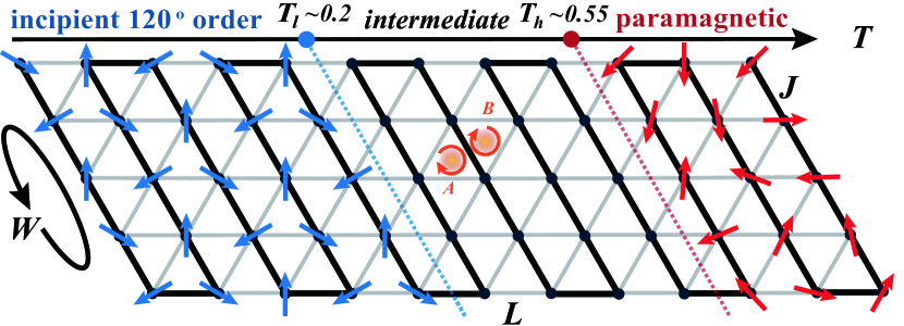
In contrast, the thermodynamics of the TLH strikingly differs in many respects from that of SLH. Based on high-temperature series expansion (HTSE) results, both models show $c_{V}$ peaks at similar temperatures, $T_{h}\simeq 0.55$ (TLH) and $T_{s}\simeq 0.6$ (SLH). The SLH enters the RC regime for $T\lesssim T_{s}$ Beard et al. (1998); Kim and Troyer (1998), whereas the TLH shows no signature for incipient order and possesses anomalously large entropies at temperatures below $T_{h}$ Elstner et al. (1994).

The classical SLH and TLH models have a similar spin stiffness $\rho_{s}$, and thus a similar constant, $C_{\xi}{\sim}\rho_{s}$, in the correlation length, $\xi{\sim}\exp{(\frac{C_{\xi}}{T})}$, as well as in the static structure factor at the ordering wave vector, $S(K){\sim}\exp{(\frac{2C_{\xi}}{T})}$, with $C_{\xi}{=}2\pi\rho_{s}{=}1.571$ (SLH) Singh and Huse (1989) and $C_{\xi}{=}4\pi\rho_{s}{=}1.748$ (TLH) Elstner et al. (1993); Zheng et al. (2006a); Azaria et al. (1992) in units of spin coupling $J$. However, the constant $C_{\xi}$ is significantly renormalized by quantum fluctuations. For the SLH, the constant is reduced by about 30% to $C_{\xi}{\sim}1.13$, while in the TLH it is reduced by an order of magnitude down to $C_{\xi}{\sim}0.1$ Elstner et al. (1993, 1994). The energy scale $E_{\mathrm{RC}}\equiv 2C_{\xi}$ naturally represents the onset of RC behavior and thus incipient order. Recent sign-blessing bold diagrammatic Monte Carlo (BDMC) simulations still show that the thermal states down to the lowest accessible temperatures $T=0.375$ “extrapolate” to a disordered ground state via a quantum-to-classical correspondence Kulagin et al. (2013).

Here, we exploit two renormalization group (RG) techniques based on thermal tensor network states (TNSs) Li et al. (2011); Chen et al. (2017, 2018): the exponential tensor RG (XTRG) which we recently introduced based on one-dimensional (1D) matrix product operators (MPOs) Chen et al. (2018), and a tensor product operator (TPO) approach Li et al. (2011). XTRG is employed to simulate the TLH down to temperatures $T<0.1$ on YC $W(\times L)$ geometries (see Fig. 1) up to width $W=6$ with default $L=2W$, and open strips [OS $W(\times L)$] with fully open boundary conditions (OBCs) and default $L=W$ Sup .

TLH thermodynamics. In Fig. 2 we present our thermodynamical results from XTRG on cylinder (YC) and open geometries (OS), as defined earlier. In Fig. 2(a), we observe from YC5, OS6, and YC6 data that, besides a high temperature round peak at $T_{h}\sim 0.55$, our YC data exhibit another peak (shoulder for OS6) at $T_{l}\sim 0.2$. On YCs, the peak position $T_{l}$ stays nearly the same when increasing $W$ from 5 to 6, also consistent with the shoulder in OS6 as well as in the experimental data. At the same time, the low-temperature peak becomes slightly weakened, yet towards the experimental data. When compared to the two virtually coinciding experimental data sets, YC6, TPO, earlier HTSE Elstner et al. (1993), and latest Padé [6,6] data Rawl et al. (2017) all agree well for $T\gtrsim T_{h}$ and reproduce the round peak of $c_{V}$ at $T_{h}$.

The remarkable agreement of finite-size XTRG with experimental measurements can be ascribed to a short correlation length $\xi\lesssim 1$ lattice spacing for $T\gtrsim 0.4$ Sup . Deviations from experiment only take place below $T_{l}$, suggesting significant finite-size effects due to larger $\xi$ in that regime. Moreover, we have checked the dependence of $T_{l}$ on the cylinder length $L$ for YC6, and find that the lower peak even gets slightly enhanced as $L$ increases. In addition to YC and OS geometries, simulations on X cylinders also lead to the same scenario Sup .

Figure 2: (Color online) Simulated thermodynamics in comparison to experimental measurements, Cui et al. (2018) Cui et al. (2018) and Rawl et al. (2017) Rawl et al. (2017), as well as earlier numerical results. The YC and OS data are obtained via XTRG by retaining up to $D^{\ast}=1000$ multiplets [$D\sim 4000$ U(1) states], and by a TPO method Sup on infinite lattices, keeping up to 40 bond states. (a) Specific heat, $c_{V}$, results benchmarked against HTSE Elstner et al. (1993); Rawl et al. (2017) and experimental curves. (b) The thermal entropy $S$ vs $T$, together with the reconstructed Schwinger boson mean field (RSBMF) Mezio et al. (2012), and “roton” contributions Zheng et al. (2006a). (c) Uniform magnetic susceptibility $T\!\chi_{0}$ vs $T$, shown with BDMC data Kulagin et al. (2013). The left top inset compares $\chi_{0}$ to Curie-Weiss (CW) $\chi_{0}=C/(T+\theta)$ in a wide temperature range, where $C=1/4$ and $\theta=2.06$. In the right bottom inset we further compare various $T\!\chi_{0}$ values at $T=0.5$. The magnetic moment per Co is assumed $\simeq 2\mu_{B}$, with Landé factor $g\simeq 4.13$ Cui et al. (2018).

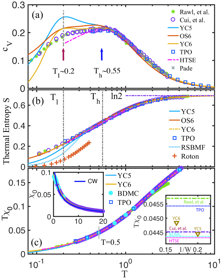
In Fig. 2(b), we present our data on thermal entropy, again directly juxtaposed with experimental as well as previous theoretical results. Whereas the YC5 data deviate at $T\lesssim 0.3$ due to finite-size effects, we observe good agreement between the two experimental data sets with our TPO results down to $T_{l}$, and with $W=6$ data (OS6 and YC6) down to the lowest temperatures in the measurements. Notably, the thermal entropy per site $S$ is about 1/3 of the high-$T$ limit, $S_{\infty}=\ln{2}$, at temperatures as low as $T\simeq 0.2$ where, for comparison, for SLH $S$ is almost zero at the same temperature Elstner et al. (1994). We emphasize that Fig. 2(b) is a direct comparison without any fitting, since the only parameter $J$ has also been determined and thus fixed as 1.66 K in the experiments Rawl et al. (2017); Cui et al. (2018). Nevertheless, since the experimental data of $S$ are determined by integrating $c_{V}/T$, starting from the lowest accessible temperature $T_{x}$, systematic vertical shifts for the curves from Refs. Rawl et al. (2017) and Cui et al. (2018) are necessary to reach the known large-$T$ limits. This results in residual entropies of $S(T_{x})=0.045$ and $0.06$ at temperatures $T_{x}=0.06$ and $0.08$ K, for Refs. Rawl et al. (2017) and Cui et al. (2018), respectively. Note that the large entropy due to quantum frustration at low $T$ is not properly described in previous theories, e.g., RSBMF Mezio et al. (2011, 2012) as shown in Fig. 2(b).

Figure 2(c) presents our results for the average magnetic susceptibility. Both data sets, YC5 and YC6, agree quantitatively with the experimental results, as well as HTSE data Elstner et al. (1993), from high temperatures down to $T\lesssim 0.1$, well beyond state-of-the-art BDMC results that reach down to $T=0.375$ Kulagin et al. (2013). In the left top inset of Fig. 2(c), we also include a Curie-Weiss (CW) fit for $T\gtrsim 1$, resulting in the positive Weiss constant $\theta\approx 2J$. In the right bottom inset, we compare the $T\!\chi_{0}$ value at $T=0.5$, and find the various numerical and experimental results all agree, up to three significant digits.

Two-temperature scales. As schematically depicted in Fig. 1, we uncover a two-temperature-scale scenario in the TLH. This confirms that the 120^∘ order plus magnon excitations is not sufficient to describe TLH thermodynamics. References. Zheng et al. (2006b); Starykh et al. (2006) argued that the TLH also has additional types of excitations which are gapped, with the minimum of their quadratic dispersion at finite momentum, and referred to these as “rotonlike excitations” (RLEs), since their dispersions are reminiscent of that known for vortexlike excitations in He⁴ Feynman (1954). Excitations with this type of dispersion have recently also been observed in neutron scattering experiments of TLH materials Ma et al. (2016); Ito et al. (2017). RLEs evidently play an important role in the intermediate-temperature regime in Fig. 1, but their precise nature has not yet been fully elucidated.

RLEs, although missed in the linear spin-wave theory, can be well captured by including $1/S$ corrections in calculating the magnon dispersions Starykh et al. (2006); Chernyshev and Zhitomirsky (2006, 2009) and dynamical correlations Mourigal et al. (2013); Luo et al. (2015). Other proposals have also been put forward to understand RLEs, including the vortex-antivortex excitation Alicea et al. (2006) with signatures already in the classical TLH phase diagram versus finite temperature Kawamura et al. (2010); Gvozdikova et al. (2011); Seabra et al. (2011); Popov et al. (2017), (nearly deconfined) spinon-antispinon pair Zheng et al. (2006b, a); Piazza et al. (2014), and magnon-interaction-stabilised excitations Mourigal et al. (2013); Verresen et al. (2018a, b).

First, the RLE quadratic band with a finite gap $\Delta{\sim}0.55\,J$ contributes to a very prominent peak in the density of states around $\Delta$ Zheng et al. (2006a). This coincides with the high-temperature scale $T_{h}\sim\Delta$ here. Therefore a possible connection of RLEs to the thermodynamic anomaly in TLH has been suggested earlier Zheng et al. (2006a); Chernyshev and Zhitomirsky (2009). Second, the RLEs themselves only start to significantly contribute to the entropy above $T_{l}$ [‘Roton’ entry in Fig. 2(b), with data taken from Ref. Zheng et al. (2006a)]. This suggests that the RLEs are activated in the intermediate temperature regime, i.e., $T_{l}\lesssim T\lesssim T_{h}$. Consequently, the onset of incipient magnetic order is postponed to a clearly lower temperature $T_{l}\sim 0.2$, which is remarkably close to previous HTSE studies, where $E_{\mathrm{RC}}\sim 0.2\,J$ sets the energy scale of classical correlation Elstner et al. (1993) as discussed earlier.

Figure 3: (Color online) (a-d) Structure factor on YC$6\times 12$ lattice, i.e., with $q_{y}$ pointing along the direction of the cylinder, at temperatures $T=5$, $0.54$, $0.2$, and $0.1$, respectively, [vertical gray lines in (e)]. (e) $S(q)$ vs $T$ at momenta $q=K$ and $M$ where the legend holds for both data sets. (f) $S_{E}$ vs $T$, where the tilted dashed lines indicate the logarithmic scaling $S_{E}=a\ln(\beta)+b$, where the slopes $a$ seen for the TLH are similar to that for the SLH (SC6 data). The vertical dashed line labels the low-temperature scale $T_{l}\sim 0.2$ for TLH and the only temperature scale $T_{s}\sim 0.6$ for SLH. SC$6\times 12$ stands for a $W=6,L=12$ square cylinder, and $S_{E}$ scaling in the Heisenberg chain (length $L=200$) is also plotted as a comparison.

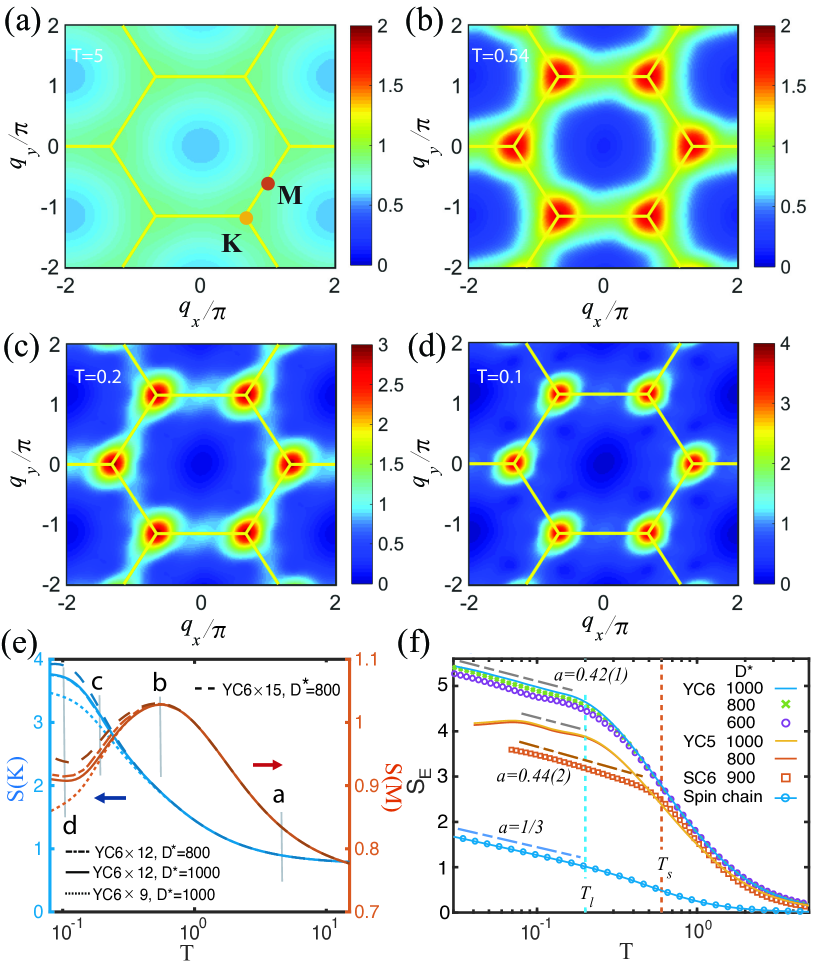
Spin structure factors. In order to shed light into the spin configurations across the intermediate regime, we turn to the temperature dependent static structure factor, $S(q)\equiv\sum_{j}e^{-iq\cdot r_{0j}}\,\langle{\mathbf{S}}_{0}\cdot\mathbb{S}_{j}\rangle_{T}$ where $r_{0j}\equiv r_{j}-r_{0}$ with $r_{j}$ the lattice location of site $j$, and $S(q)\in\mathbb{R}$ due to lattice inversion symmetry. There are two further high-symmetry points of interest, $q=K$ and $M$, as marked in Fig. 3(a). Up to symmetric reflections, $K{\equiv}(\frac{2\pi}{3},\frac{2\pi}{\sqrt{3}})$ relates to $120^{\circ}$ non-collinear order, whereas $M{\equiv}(0,\frac{2\pi}{\sqrt{3}})$ relates to nearest-neighbor (stripe) AF correlations. The latter have also been related to RLEs which feature band minima at the $M$ points Zheng et al. (2006b); Starykh et al. (2006); Ghioldi et al. (2018).

In Figs. 3(a-d) we show the overall landscape of $S(q)$. With decreasing temperature, $S(q)$ changes from rather featureless in Fig. 3(a), to showing bright regions in the vicinity of the six equivalent $K$ points as well as enhanced intensity at the $M$ points at $T\sim T_{h}$ in Fig. 3(b). Even at $T\sim T_{l}$ in Fig. 3(c), one can still recognize an enhanced intensity $S(M)$, which fades out eventually when $T$ is decreased below $T_{l}$ in Fig. 3(d). A quantitative comparison is given in Fig. 3(e).

From Fig. 3(e), we observe that $S(K)$ increases monotonously as $T$ decreases. It is featureless around $T_{h}$, and eventually saturates at the lowest $T$ due to finite system size. For $T>T_{l}$, $S(K)$ increases only slowly with decreasing temperature, and is independent of length $L$. It therefore shows no signature of incipient order there. For $T<T_{l}$, $S(K)$ rapidly increases, which eventually saturates with decreasing $T$ in an $L$-dependent manner, due to finite-size effects.

Furthermore, we observe from Fig. 3(e) that $S(M)$ develops a well-pronounced maximum around $T_{h}$. The maximum is already stable with system size, hence can be considered a feature in the thermodynamic limit. This is consistent with a picture that RLEs are activated near the $M$ points.

MPO entanglement. The two-energy-scale scenario also leaves a characteristic trace in the entanglement entropy $S_{E}$, computed at a bond (near the center) of the MPO Verstraete et al. (2004); Feiguin and White (2005); Chen et al. (2018). Gapless low-energy excitations in 1+1D conformal field theory (CFT) can give rise to a logarithmic increase of the entanglement, $S_{E}\propto-\frac{c}{3}\ln{T}$ with $c$ the conformal central charge Barthel ; Dubail (2017); Chen et al. (2018). One can also observe logarithmic $S_{E}$ behavior in the 2D SLH model, related to the spontaneous SU(2) symmetry breaking (at $T=0$) Chen et al. (2018), as also added for reference (“SC6” data) in Fig. 3(f).

We find similar behavior of the $S_{E}$ profiles of the TLH on YC5 and YC6 geometries in Fig. 3(f) down to $T=0.04$, with bond dimension $D^{\ast}\lesssim 1000$ multiplets ($D\sim 4D^{\ast}$ states). Interestingly, the lower-energy scale $T_{l}\sim 0.2$ (vertical dashed line) signals the onset of logarithmic entanglement scaling versus $T$, which in agreement with Fig. 2(a) already coincides for $W=5$ and $6$. For YC5, the window with logarithmic entanglement is rather narrow, below of which $S_{E}$ saturates as we already approach the ground state. For YC6, the entanglement continues to increase down to our lowest temperature $T=0.03$. We associate the logarithmic $S_{E}$ behavior with the onset of incipient order, which is closely related to SU(2) symmetry breaking at $T=0$ that gives rise, e.g., to a $1/(N=LW)$ level spacing in the low-energy tower of states Bernu et al. (1992). Concomitantly, we also observe a qualitative change of behaviors in the entanglement spectra at $T_{l}$ Sup .

Scalar chiral correlations.

Figure 4: (Color online) Chiral correlations on cylinders, YC5 and YC6 (for YC4, see Ref. Sup ). The inset represents the eigenstates $\Psi$ (and $\Psi^{\ast}$) of the chiral operator $\chi$ (Fig. 1) with non-zero eigenvalues $\pm\sqrt{12}$. They have total spin $S=1/2$, and hence are superpositions of configurations with two-site singlet dimers (thick lines) whose signs are fixed in clockwise order (arrow). Having $\alpha=\exp(2\pi i/3)$, this demonstrates the chiral nature.

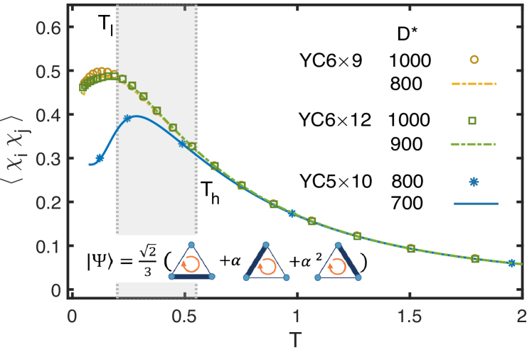
Chiral correlations in the TLH have raised great interest since the proposal of a Kalmeyer-Laughlin chiral spin liquid Kalmeyer and Laughlin (1987). Intriguingly, recent $T=0$ studies on the fermionic triangular lattice Hubbard model proposed a chiral intermediate phase versus Coulomb repulsion which thus breaks time reversal symmetry Szasz et al. (2018). While debated Shirakawa et al. (2017), we take this as a strong motivation to also study traces of chiral correlations in the TLH at finite $T$.

In Fig. 4, we present the chiral correlation $\langle\chi_{i}\chi_{j}\rangle$ between two nearest-triangles $i,j$ in the system center, as defined with Fig. 1. This shows that chiral correlations are weak in both high- and low-temperature limit, while they become strong Szasz et al. (2018) in the intermediate temperature regime, with a peak around $T_{l}$. Below $T_{l}$, the chiral correlations drop strongly, giving way to the buildup of coplanar incipient order.

Discussion. Our study suggests a tight connection between RLEs and chiral correlations in the intermediate regime $T_{l}\lesssim T\lesssim T_{h}$ (cf. Fig. 4). In this sense, we speculate that RLEs activated in the intermediate-temperature regime indicate phase-coherent rotating dimers, as schematically sketched with Fig. 4. Given that the complex phase of the dimers “rotates” by $2\pi$, this suggests a possible link to a topological, vortexlike nature of the RLEs. Moreover, it resembles Feynman’s notion of rotons in terms of quantized vortices in He⁴ Feynman (1954) via an exact mapping of TLH to a system of hardcore bosons. The latter further underlines the striking analogy between the anomalous thermodynamics of the TLH and the renowned roton thermodynamics in He⁴ H. C. Kramers and Gorter (1952); Bendt et al. (1959).

The low-energy scale $T_{l}$ can be tuned by deforming the Hamiltonian, e.g., by altering the level of frustration by adding a next-nearest $J_{2}$ coupling to the TLH. We see that increasing $J_{2}$ reduces $T_{l}$, as well as the height of the corresponding peak in the specific heat, suggesting that the RLE gap is decreasing and the influence can thus spread down to even lower-temperature/energy scales, in consistency with dynamical studies of the $J_{1}$-$J_{2}$ TLH Ghioldi et al. (2015); Ferrari and Becca (2019). In addition, TLH can be continuously deformed into the SLH, where $T_{l}$ increases and eventually merges with $T_{h}$ once sufficiently close to the SLH. We refer more details to the Supplemental Materials Sup .

Outlook. A detailed study of the microscopic nature of RLEs, e.g., via dynamical correlations at finite temperature, is beyond the scope of the present paper, and is thus left for future research. Further stimulating insights and possible superfluid analogies are also expected from an analysis of the interplay of external magnetic fields and thermal fluctuations in TLH Griset et al. (2011); Starykh (2015) with clear experimental relevance Cui et al. (2018).

I Finite-Temperature Renormalization Group Approaches

In this section, we recapitulate the two thermal tensor network approaches employed in the present study, i.e, the exponential tensor renormalization group (XTRG) based on matrix product operators (MPOs) and the tensor product operator (TPO) approach. The former is highly controllable while restricted to finite-size systems; the latter can be applied directly in the thermodynamic limit, but is constrained by finite bond dimensions as well as an approximate optimization scheme. Nevertheless, we exploit a combination of 1D/2D tensor network RG approaches to study the triangular lattice Heisenberg (TLH) model, and find the results of the two methods consistent.

I.1 Exponential Tensor Renormalization Group: A matrix product operator approach

Figure S1: (Color online) (a) Exponential vs. linear thermal evolution of the unnormalized density operator, $\rho\equiv e^{-\beta H}$. (b) The procedure of MPO doubling in XTRG, i.e. $\rho_{n+1}=\rho_{n}\ast\rho_{n}$ corresponding to $\beta_{n+1}=2\beta_{n}=2^{n}\tau_{0}$.

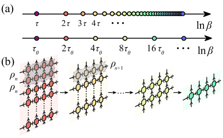
We start from the MPO-based XTRG approach, which was proposed in Ref. Chen et al. (2018). There the (unnormalized) thermal mixed state $\rho({\beta})\equiv e^{-\beta H}$ of the system is represented as 1D MPO, as depicted in Fig. S1(b). In the purification framework, $\rho({\beta})$ represents a thermo-double field, where the trace with its conjugate results in the partition function at $2\beta$, i.e.,

$$Z(2\beta)=\rm{Tr}[\rho(\beta)\cdot\rho^{\dagger}(\beta)].$$ (S1)

Similarly, one can compute thermodynamic quantities. While equivalent to the concept of purification, we emphasize, however, that here we always describe the density matrix as an MPO and thus as an operator. The added benefit of using $\rho\rho^{\dagger}$ as in Eq. (S1) is that it always yields a positive and, thus, a physical thermal density operator at inverse temperature $2\beta$.

The evolution of $\rho(\beta)$ always starts from infinite temperature in thermal RG approaches, where the density operator is just a trivial identity, i.e. $\rho(0)=\mathbb{I}$. Conventional linear RG approaches evolve the density matrix linearly in $\beta$, i.e.,

$$\rho(n\tau)=\underset{n}{\underbrace{\rho(\tau)\cdot\rho(\tau)\cdot...\cdot\rho(\tau)}}\cdot I\,,$$ (S2)

where $\tau$ is a small imaginary time (inverse temperature) step size that applies to all $\beta_{n+1}=\beta_{n}+\tau$. We refer to such a scheme, schematically depicted in the upper row of Fig. S1(a), as a linear thermal RG, see Ref. Li et al. (2011).

A recent insight from the logarithmic entanglement scaling in conformal field theory proves that the block-entanglement growth in a thermal MPO is upper bounded by $S_{E}\leq a\ln\beta+b$ with some constants $a$ and $b$ Barthel ; Dubail (2017). This shows that the entanglement entropy $S_{E}$ of the MPO actually changes significantly only when $\beta$ changes by a factor. In light of this, the linear evolution is realized to be a very slow cooling procedure, while a more efficient way is to follow the logarithmic temperature scale. A particularly simple and convenient choice is $\beta\to 2\beta$, i.e.,

$$\rho_{n+1}=\rho_{n}\ast\rho_{n},$$ (S3)

with $\rho_{n}\equiv\rho(2^{n}\tau_{0})$, and $\tau_{0}$ an arbitrarily small initial starting point. The asterisk here is a reminder to emphasize the underlying MPO product structure. This exponential procedure is illustrated in lower row of Fig. S1(a), as well as in Fig. S1(b), which reveal manifestly the efficiency of XTRG, i.e., the system reaches the lowest temperature exponentially fast. Similarly, by its very construction, XTRG can also start from an arbitrarily small $\tau_{0}$, which thus allows one to resort to a very simple but accurate initialization of $\rho_{0}$, e.g. using series expansion,

$$\rho_{0}\equiv\rho(\tau_{0})=\sum_{n=0}^{n_{c}}\frac{(-\tau_{0})^{n}}{n!}H^{n},$$ (S4)

even using a cutoff as small as $n_{c}=1$ where the MPO for $\rho_{0}$ is given – up to a very minor adaptation – by the MPO of $H$ itself with the same bond dimension. For comparison, $n_{c}=2$ only includes one further doubling of the MPO of $H$ with itself, an elementary MPO procedure in XTRG in any case. Overall, the techniques required to perform the expansion in Eq. (S4) have been developed in Ref. Chen et al. (2017), dubbed as series-expansion thermal tensor network (SETTN) method.

Naively, one might expect that the numerical cost for the step in Eq. (S3) scales like $\mathcal{O}(D^{6})$ with $D$ the bond dimension of MPO, and thus represents a (prohibitively) expensive calculation. The numerical cost, however, can be strongly reduced to $\mathcal{O}(D^{4})$ by resorting to a variational procedure (see Chen et al. (2017) for details), thus allowing larger $D$ in the calculation. In addition, thanks to the versatile QSpace framework Weichselbaum (2012), we have fully implemented non-Abelian symmetries in our XTRG simulations which effectively reduces the bond dimension by switching from $D$ states to $D^{\ast}$ multiplets. Conversely, for the case of SU(2) in the present study, we can therefore keep up to $D\lesssim 4\times D^{\ast}$ individual U(1) states.

Finally, we would like to emphasize that XTRG is not only superior to conventional linear RG in efficiency, but also in terms of accuracy. Since the lowest temperature can be reached in an extremely speedy fashion, this results in a significantly smaller number of numerical iterations. Hence also the truncation error accumulation is greatly reduced. A detailed comparison of accuracies and efficiencies between XTRG and LTRG, as well as SETTN, also can be found in Ref. Chen et al. (2018).

I.2 Tensor Product Operator Approach

As an alternative approach in our simulations, we also utilize the tensor product operator (TPO) approach, whose results generally are in agreement with XTRG. Here we provide details of our TPO algorithm together with more benchmark calculations. For practical and historical reasons, we still use a numerical code that is based on a linearized scheme in the imaginary time evolution based on Trotter decomposition in our TPO algorithm, and also does not yet exploit any symmetries. Its concepts, nevertheless, can equally well be generalized in the spirit of doubling of the density matrix as in XTRG.

Figure S2: (Color online) The triangular lattice (dashed lines) represented in the TPO ansatz (thick lines with symbols for tensors). Since we use Trotter decomposition within our TPO simulations, we need to differentiate sets of three tensors. There are three kinds of rank-5 tensors, i.e. tensors with five external indices, namely $T_{a}$, $T_{b}$ and $T_{c}$ (orange, green, and blue triangles, respectively) located on the sites of the TLH, where the two physical indices for bra and ket, i.e. $\sigma$ and $\sigma^{\prime}$, are omitted for simplicity. There are also three kinds of rank-3 intermediate tensors $S_{a}$, $S_{b}$ and $S_{c}$ (orange, green, and blue circles, respectively), without physical indices, residing in the center of the face of the up-triangles in the TLH. The geometrical bonds can be grouped by their orientation, labelled $x$, $y$ and $z$. The two horizontal dashed blue lines denote the XC boundary condition, where the system is wrapped up vertically (having $W=4$ in the plot above). The two vertical lines indicate the transfer matrix $T_{m}$ along the cylinder where, by definition of a transfer matrix, all ‘internal’ indices, including the physical indices as well as intermediate geometric indices, should be traced, with the only open indices the thick lines crossing the vertical dashed lines.

I.2.1 TPO Representation of the Density Matrix

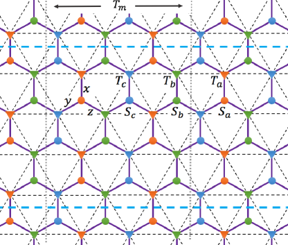
From a numerical efficiency point of view, it is favorable to describe the thermal states of TLH via an effective hexagonal lattice TN, as shown in Fig. S2. Furthermore, given that the TLH carries a $120^{\circ}$ magnetic order at zero temperature, this naturally divides the sites on the TLH into three sublattices, which is also required for a Trotter decomposition in any case. Therefore we introduce three types of $T$ tensors, $T_{a}$, $T_{b}$, and $T_{c}$ on the $A$-, $B$-, and $C$-sites (orange, green and blue solid triangles in Fig. S2, respectively). All of them are rank-5 tensors with 2 physical indices and 3 geometric ones. The $T$ tensors are interconnected to form the hexagonal tensor network (TN) in Fig. S2 along the $x$-, $y$-, $z$-bonds via three types of rank-3 $S$ tensors, $S_{a}$, $S_{b}$ and $S_{c}$ (orange, green and blue solid circles, respectively) with no physical indices of their own. The $S$ tensors reside on three distinct up-triangles, dubbed as $a$-, $b$-, and $c$-triangles, corresponding to the three sublattices $A$, $B$, and $C$, respectively. They contain disconnected subsets of nearest-neighbor terms on the TLH which can be readily utilized for a Trotter decomposition [cf. Eq. (S6)]. In Fig. S2 we also indicate how to wrap up the TPO on an XC, i.e., by imposing periodic boundary condition (BC) along the vertical direction.

Throughout, we assume that the (starting) configuration of the $S$ tensors is in the canonical form,

$$\sum_{i,j}(S_{\alpha})^{*}_{ijk}(S_{\alpha})_{ijk^{\prime}}=(\lambda^{\alpha}_{k})^{2}\delta_{kk^{\prime}}.$$ (S5)

where the $\alpha\in a,b,c$ labels different $S$ tensors, and the bond indices $(i,j,k)$ denotes cyclic permutations of $(x,y,z)$. This form can be achieved by higher-order singular-value decomposition (HOSVD), with a residual unitary out of the $S$ tensors absorbed into the $T$ tensors, and the singular values $\lambda^{\alpha}_{k}\geq 0$ reabsorbed into the $S$ tensor. The contraction in Eq. (S5) thus regenerates a diagonal matrix with entries $(\lambda^{\alpha}_{k})^{2}$. For a more detailed discussion of HOSVD, we refer the reader to Refs. Lathauwer et al. (2000); Xie et al. (2014)

Figure S3: (Color online) Procedure of a single projection step: (a) Absorptions of $\lambda$ matrices, where the suggestive arrow with the $\lambda$’s indicates the (approximate) orthonormalization of the entire Bethe TNS. (b) QR decomposition, while also splitting off the upper physical indices. (c) Applying the triangular imaginary time step $e^{-\tau h}$ to the base tensor. (d) HOSVD of the base tensor. (e) truncate and update $S_{a}$ as well as three $T$ tensors.

I.2.2 Imaginary-time Evolution and Simple Update Scheme of TPO

We utilize the Bethe-lattice approximation, also referred to as simple update Jiang et al. (2008); Li et al. (2012), in the imaginary-time evolution to optimize the TPO density matrix of the system from high to low temperatures. To be concrete, via a Trotter-Suzuki decomposition, the density matrix can be expressed as

$$\rho=e^{-\beta H}\approx\bigl{(}e^{-\tau H^{A}}e^{-\tau H^{B}}e^{-\tau H^{C}}\bigr{)}^{N}\equiv\bigl{(}P^{A}P^{B}P^{C}\bigr{)}^{N}\quad\text{with}\quad P^{\Lambda}\equiv\prod_{i\in\Lambda}e^{-\tau h_{i}},$$ (S6)

where $H^{\Lambda}\equiv\sum_{i\in\Lambda}h_{i}$, with $h_{i}$ the ‘triangular plaquette’ Hamiltonian on the up-triangle $i$ in sublattice $\Lambda\in A,B,C$, and $\tau$ the Trotter step (chosen as $0.01\sim 0.02$ in practice). By construction, $[h_{i},h_{i^{\prime}}]=0$ for $i\neq i^{\prime}$ within the same sublattice $i,i^{\prime}\in\Lambda$. All of the $h_{i}$ have identical form for the isotropic Heisenberg model considered here. We initialize with an infinite-temperature density matrix (direct product of identities), and apply the triangular operators $P^{\Lambda}$ sequentially for $\Lambda\in A,B,C$. This is repeated iteratively to cool down the TPO density matrix.

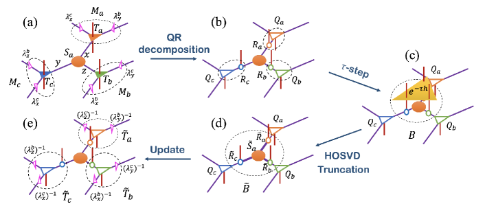
To be specific, we now describe in detail the application of $P^{A}$, where the tensor $S_{a}$ is surrounded by the tensors $T_{a}$, $T_{b}$ and $T_{c}$ (see Fig. S2 and also Fig. S3).

1. We firstly (re)generate the diagonal $\lambda^{\alpha}$ matrices as in Eq. (S5) out of the $S_{\alpha}$ tensors surrounding the $T$ tensors,
   i.e. $\alpha\in\{b,c\}$.

2. Next we absorb the $\lambda$’s into the $T$’s to construct the tensors $M$ [Fig. S3(a)]

   $$(M_{a})^{\sigma_{a}^{\prime}\sigma_{a}}_{xyz} = (T_{a})^{\sigma_{a}^{\prime}\sigma_{a}}_{xyz}\lambda_{y}^{b}\lambda_{z}^{c},$$ (S7a)

   $$(M_{b})^{\sigma_{b}^{\prime}\sigma_{b}}_{xyz} = (T_{b})^{\sigma_{b}^{\prime}\sigma_{b}}_{xyz}\lambda_{x}^{b}\lambda_{y}^{c},$$ (S7b)

   $$(M_{c})^{\sigma_{c}^{\prime}\sigma_{c}}_{xyz} = (T_{c})^{\sigma_{c}^{\prime}\sigma_{c}}_{xyz}\lambda_{z}^{b}\lambda_{x}^{c}$$ (S7c)

   (note that we explicitly indicate summation, i.e. there is no implicit summation here over double indices since the $\lambda$ matrices are diagonal).

3. Perform QR decompositions of $M_{a}$, $M_{b}$ and $M_{c}$ [Fig. S3(b)]

   $$(M_{a})^{\sigma_{a}^{\prime}\sigma_{a}}_{x^{\prime}yz} = \sum_{x}(Q_{a})^{\sigma_{a}^{\prime}}_{xyz}(R_{a})^{\sigma_{a}}_{xx^{\prime}},$$ (S8a)

   $$(M_{b})^{\sigma_{b}^{\prime}\sigma_{b}}_{xyz^{\prime}} = \sum_{z}(Q_{b})^{\sigma_{b}^{\prime}}_{xyz}(R_{b})^{\sigma_{b}}_{zz^{\prime}},$$ (S8b)

   $$(M_{c})^{\sigma_{c}^{\prime}\sigma_{c}}_{xy^{\prime}z} = \sum_{y}(Q_{c})^{\sigma_{c}^{\prime}}_{xyz}(R_{c})^{\sigma_{c}}_{yy^{\prime}}.$$ (S8c)

   Here we have also split off the upper physical indices into the tensors $R_{a}$, $R_{b}$ and $R_{c}$ which significantly reduces the computational cost in the projection-truncation procedure in the next step.

4. Construct the base tensor $B$ by contracting $R_{a}$, $R_{b}$, $R_{c}$ with $S_{a}$ tensor

   $$B^{\sigma_{a}\sigma_{b}\sigma_{c}}_{xyz}=\sum_{x^{\prime},y^{\prime},z^{\prime}}(R_{a})^{\sigma_{a}}_{xx^{\prime}}(R_{b})^{\sigma_{b}}_{zz^{\prime}}(R_{c})^{\sigma_{c}}_{yy^{\prime}}(S_{a})_{x^{\prime}y^{\prime}z^{\prime}},$$ (S9a)

   and apply the 3-site imaginary-time step $$P=e^{-\tau h}$$ onto the base tensor [Fig. S3(c)]

   $$\tilde{B}^{\sigma_{a}\sigma_{b}\sigma_{c}}_{xyz}=\sum_{\sigma^{\prime}_{a},\sigma^{\prime}_{b},\sigma^{\prime}_{c}}P^{\sigma_{a}\sigma_{b}\sigma_{c}}_{\sigma^{\prime}_{a}\sigma^{\prime}_{b}\sigma^{\prime}_{c}}\cdot B^{\sigma^{\prime}_{a}\sigma^{\prime}_{b}\sigma^{\prime}_{c}}_{xyz}.$$ (S9b)

5. Take HOSVD of the modified base tensor $\tilde{B}$ by performing independent SVD w.r.t. the index pairs $(\sigma_{a},x)$, $(\sigma_{b},z)$, and $(\sigma_{c},y)$, providing the isometries $\tilde{R}_{a}$ to $\tilde{R}_{c}$, respectively [Fig. S3(d)]. Then by projecting the original tensor $\tilde{B}$ with $\tilde{P}_{\alpha}\equiv\tilde{R}_{\alpha}\tilde{R}_{\alpha}^{\dagger}$ on all three indices $\alpha\in\{a,b,c\}$, one obtains the updated tensor $\tilde{S}$,

   $$(\tilde{S}_{a})_{xyz}=\sum_{\begin{subarray}{c}\sigma_{a}\sigma_{b}\sigma_{c}\\ x^{\prime}y^{\prime}z^{\prime}\end{subarray}}(\tilde{R}_{a}^{\ast})^{\sigma_{a}}_{x^{\prime}x}(\tilde{R}_{b}^{\ast})^{\sigma_{b}}_{z^{\prime}z}(\tilde{R}_{c}^{\ast})^{\sigma_{c}}_{y^{\prime}y}\tilde{B}_{x^{\prime}y^{\prime}z^{\prime}}^{\sigma_{a}\sigma_{b}\sigma_{c}},$$ (S10a)

   or equivalently,

   $$\tilde{B}^{\sigma_{a}\sigma_{b}\sigma_{c}}_{xyz}=\sum_{x^{\prime},y^{\prime},z^{\prime}}(\tilde{R}_{a})^{\sigma_{a}}_{xx^{\prime}}(\tilde{R}_{b})^{\sigma_{b}}_{zz^{\prime}}(\tilde{R}_{c})^{\sigma_{c}}_{yy^{\prime}}(\tilde{S}_{a})_{x^{\prime}y^{\prime}z^{\prime}}.$$ (S10b)

   In exact numerics, the bond dimensions of $\tilde{S_{a}}$ would be generally enlarged by the local Hilbert space dimension $d$, and thus needs to be truncated. This is achieved by discarding the smallest singular values in $\lambda$, such that $\tilde{P}_{\alpha}$ becomes a true projector, namely to the sector of dominant singular values. The kept singular values are the ones that also occur in Eq. (S5). Without symmetry breaking, the three directions $x,y,z$ are equivalent, and hence the $S$ and $T$ tensors may be chosen symmetric under cyclic permutation of these indices, throughout. This simplifies the TPO step above in that only a single SVD already suffices to obtain $\tilde{R}\equiv\tilde{R}_{a}=\tilde{R}_{b}=\tilde{R}_{c}$. In practice, the results were equivalent whether or not this lattice symmetry was enforced.

6. The truncated $\tilde{R}$ tensors in Eq. (S10b) can now be contracted (absorbed) into the $Q$ tensors in (iii). By also undoing step (ii) by applying inverted $\lambda^{b}$ and $\lambda^{c}$ weights (note that in the above steps, only $\lambda^{a}_{\xi}$ with $\xi\in\{x,y,z\}$ was altered, but the sets $\lambda^{b}_{\xi}$ and $\lambda^{c}_{\xi}$ remained the same), we obtain the updated $\tilde{T}$ tensors [Fig. S3(e)],

   $$(\tilde{T}_{a})^{\sigma_{a}^{\prime}\sigma_{a}}_{x^{\prime}yz} = \sum_{x}(Q_{a})^{\sigma_{a}^{\prime}}_{xyz}(\tilde{R}_{a})^{\sigma_{a}}_{xx^{\prime}}/(\lambda_{y}^{b}\lambda_{z}^{c}),$$ (S11a)

   $$(\tilde{T}_{b})^{\sigma_{b}^{\prime}\sigma_{b}}_{xyz^{\prime}} = \sum_{z}(Q_{b})^{\sigma_{b}^{\prime}}_{xyz}(\tilde{R}_{b})^{\sigma_{b}}_{zz^{\prime}}/(\lambda_{x}^{b}\lambda_{y}^{c}),$$ (S11b)

   $$(\tilde{T}_{c})^{\sigma_{c}^{\prime}\sigma_{c}}_{xy^{\prime}z} = \sum_{y}(Q_{c})^{\sigma_{c}^{\prime}}_{xyz}(\tilde{R}_{c})^{\sigma_{c}}_{yy^{\prime}}/(\lambda_{z}^{b}\lambda_{x}^{c}).$$ (S11c)

I.2.3 Evaluation of thermal quantities

The $S$ and $T$ tensors from the simple update above are inserted into the 2D-TN of Fig. S2. One then needs to contract this TN efficiently in the thermodynamic limit to obtain the partition function, and thus physical thermal properties such as free energy, energy, magnetization, etc. This constitutes another essential challenge of the algorithm. For finite-size cylinders with a small width $W$, e.g., XC4, we perform exact contractions; while for an infinite-size system, we use conventional boundary matrix product state (MPS) technique adopted in infinite projected entanglement pair state (iPEPS) algorithms Jordan et al. (2008).

For both the XC4 and infinite-size systems, the dominating eigenvector as well as eigenvalue of the horizontal transfer matrix $T_{m}$ (i.e. with a cut in Y direction, see Fig. S2) can be obtained exactly (for the XC4) or approximately (for infinite systems) by iteratively contracting a trial initial vector with $T_{m}$ until convergence. For this, double-layer TPO, i.e. using $\rho(\beta/2)^{\dagger}\rho(\beta/2)\rightarrow\rho(\beta)$ to enforce positivity, is orders of magnitude more expensive as compared to the relatively cheap single-layer formalism of TPO. For the XC4 system, the single-layer TPO computations are affordable at a cost of $O(D^{6})$, where $D$ up to 60 is the bond dimension of TPO. For the subsequent embedding into an infinite 2D TNS, the TPO cost scales as $O(\chi^{3}D^{3})$, with $\chi$ the bond dimension of the boundary MPS. In practice, we choose $D$ up to 40 and $\chi\sim 4D$, which is affordable, yet also ensures data convergence over the parameter $\chi$.

Figure S4: (Color online) (a) XC geometry where the dark blue lines indicate the MPO path in the XTRG simulations. (b) Comparison of specific heat $c_{V}$ between TPO and XTRG on XC4 and, for reference, also HTSE-2D, i.e., not constrained to the XC4 geometry. The high temperature scale, $T_{h}\sim 0.55$, indicates the high temperature round peak, while the low temperature scale, $T_{l}^{*}\sim 0.28$, is slightly higher than $T_{l}\sim 0.20$ for wider systems, e.g., YC6 in the main text as well as XC6 below. (c,d) illustrate the bond energy textures on XC4 (no vertical stripes) and XC6 (vertical stripes) geometries, consistent with $T=0$ DMRG simulations Weichselbaum and White (2011). The explicit symmetry breaking in the vertical direction by forming stripes, here in (d), at finite temperature is necessarily linked to the choice of the open boundary edges.

II Triangular Lattice Antiferromagnet

II.1 Benchmark results on XC4 geometry

Figure S5: (Color online) Static structure factor $S(q)$ of XC4, i.e., with $q_{x}$ pointing along the cylinder, computed by TPO (a-d) and XTRG (e,f) at various temperatures, $T\simeq 2,0.8,0.3,0.125$, as also indicated by the vertical solid gray lines in (g). While only having $W=4$ discrete $q_{y}$ momenta due to periodic BC, we interpolate by adding further intermediate points $q_{y}$ in the Fourier transform in $S(q)$ to obtain for overall smoother results. The vertical dashed lines in (g) indicate $T_{l}$ and $T_{h}$. Overall, the TPO data in (c,d) shows good agreement with the XTRG data in (e,f) at the same respective temperatures. (g) $S(q)$ at $q=K$ and two types of $M$ points [cf. panel (a)] vs. $T$, again with good quantitative agreement between TPO and XTRG.

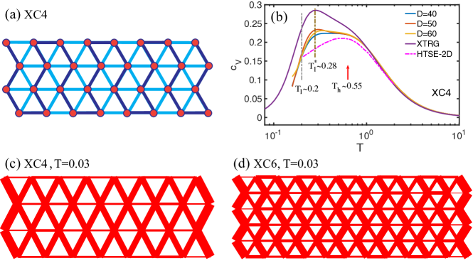
In contrast to YC geometries which correspond to a cylinder with straight ends, the XC geometry results in a cylinder with zigzag ends Weichselbaum and White (2011). Also note that the YC systems have a unique shortest distance path along the nearest-neighbor bonds of the TLH around the circumference when starting from an arbitrary but fixed lattice site. This can favor 1D RVB stripe structures around the circumference, in contrast to XC systems. Here therefore we apply both methods above to an XC4 geometry, i.e., of width $W=4$, as shown in Fig. S4(a). For XTRG, we use our default aspect ratio $L/W=2$, and map the 2D lattice into a 1D structure along the snake line also shown in Fig. S4(a). For the TPO method, we optimise the tensors $T$ and $S$ directly in the thermodynamic limit, and connect the local tensors on an infinitely long XC4 lattice.

In Fig. S4(b), the specific heat, $c_{V}$, of XC4 obtained by XTRG by retaining $D^{\ast}=400$ multiplets, and by TPO with different bond dimensions $D$ up to 60, is presented in comparison with HTSE. The two temperature scales are apparent in both cases, although the low temperature peak appears at $T_{l}^{*}\sim 0.28$ somewhat above the value $0.20$ obtained on wider YC geometries. This is due to strong finite-site effects on XC4, which will be further analyzed shortly by calculating the static structure factor $S(q)$. Another distinct feature is that the lower-temperature peaks in TPO curves are significantly lower than for the XTRG results. This may also hint a smaller finite-size effect in the TPO approach (due to its simple update scheme).

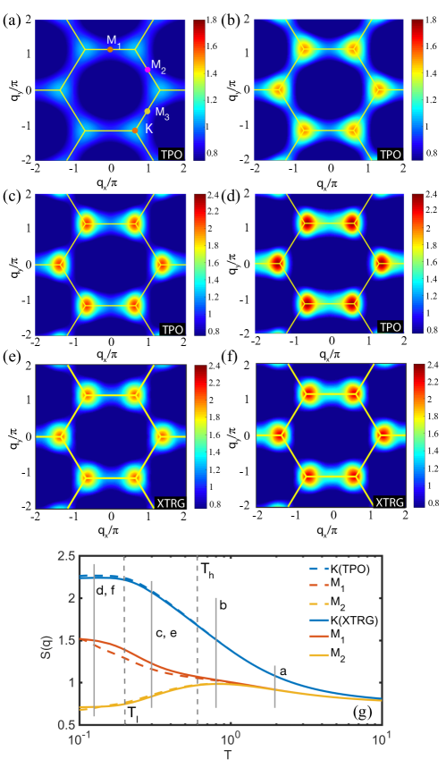
In Fig. S5(a-f), we visualize the static structure factors $S(q)$ for XC4 in the first BZ at various temperatures, which are marked by grey solid lines in Fig. S5(g) together with the corresponding panel reference [(a-d) from TPO, and (e,f) from XTRG calculations]. When lowering the temperature, the triangular lattice symmetry is broken around $T_{h}$ due to the finite system size, as manifested by the slightly different behavior of the data for the otherwise equivalent points $M_{1}$ and $M_{2}$ [indicated by markers in Fig. S5(a)]. For temperatures below $T_{h}$, one can observe that $S(M_{1})$, which points perpendicular to the direction of the cylinder, turns brighter whereas $S(M_{2})$ and $S(M_{3})$ start loosing weight. This indicates a tendency for enhanced AF, i.e. Néel like correlations around the circumference of the cylinder. Note that for XC4 one has equivalent, i.e. non-symmetry broken shortest zig-zag paths around the circumference of the cylinder [vertical direction in Fig. S4(c)].

In Fig. S5(g) we also directly compare $S(q)$ vs. $T$ at $M_{1,2}$ and $K$ from both methods, XTRG as well as TPO. At the $K$ and $M_{2}$ points, the data from the two methods coincide, while for $M_{1}$, the XTRG data reaches the low-$T$ limit faster. This may be attributed to a stronger (or cleaner) finite-size effect in XTRG, as compared to the TPO data which, despite being evaluated on a cylinder, originates from an infinite-system simple update. A similar conclusion was already drawn from the data in Fig. S4(b) regarding the higher $c_{V}$ peak for XTRG at $T_{l}^{*}$.

Figure S6: (Color online) (a) Specific heat $c_{V}$ on XC6 and YC6 lattices. (b) Static magnetic susceptibility $\chi_{0}$ vs. $T$. We also added HTSE-2D data and other data from the literature for reference, as well as a simple Curie Weiss (CW) estimate (same as in Fig. 2 in the main paper). For a discussion of numerical cost, i.e. the growth of the block entanglement $S_{E}$ with decreasing $T$, see, e.g., Fig. 3(f) in the main text.

Figure S7: (Color online) Comparison of structure factor between (a) XC$6{\times}12$ and (b) YC$6{\times}12$ geometries at $T=0.103$. The direction along the cylinder corresponds to $q_{x}$ and $q_{y}$, respectively. XC6 shows a higher intensity around $M_{1}$ which indicates a tendency to form stronger bonds around the circumference of the cylinder, i.e., stripe order. Consequently, XC6 has a lower $S(K)$ as compared to YC6, shown more explicitly in (c).

II.2 Specific heat, susceptibility, and structure factor for cylinders up to $W=6$

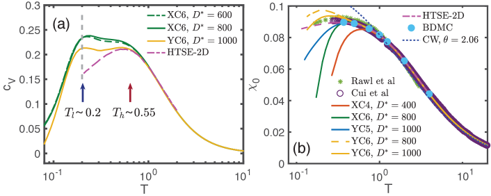
We present our XTRG results on XC6 and YC6 systems for the specific heat and static susceptibility in Fig. S6, and for the static structure factor in Fig. S7. Overall, we expect clearly reduced finite-size effects as compared to the width $W=4$ systems.

The specific heat, $c_{V}$, on XC6, shown in Fig. S6(a), agrees well with both YC6 and HTSE in the high temperature regime, $T\gtrsim T_{h}$. The observed lower energy scale in this data is stable around $T_{l}\sim 0.2$ also for this wider system. In Fig. S6(b), we compare our XTRG data for the magnetic susceptibility, $\chi_{0}$ vs. $T$, on XC6 with other results including two experimental measurements, XC4, YC5 and 6, HTSE, etc. A good agreement between XC6 data and experimental results can be observed, although YC6 produces $\chi_{0}$ mostly close to experiments and constitutes the overall most suitable geometry.

From Figs. S6(a,b) we can conclude that although XC6 has many features in common with YC6, it suffers larger finite-size effects and is less favorable in approximating the thermodynamic limit. This can be directly seen in the bond energy texture on XC6 in Fig. S4(d). Although being measured at a finite temperature, it is consistent with previous DMRG studies of the ground state properties Weichselbaum and White (2011), where spontaneous zig-zag stripe formation around the circumference of the cylinder is found for XC systems of width $2n+4$, with $n$ an integer.

The structure factor, $S(q)$, is analyzed in Fig. S7, where XC6 [Fig. S7(a)] is compared to YC6 [Fig. S7(b)]. By reaching temperatures as low as $T\sim 0.1<T_{l}$, we expect signatures of incipient $120^{\circ}$ order to be present in both systems. For YC6 cases, there exist two $M$ points ($M_{1}$ and $M_{3}$) which have strong intensity, while the remaining one, $S(M_{2})$, is weak at low temperatures, although all three $M$ points have anomalous enhancement at $T$ around $T_{h}$, due to RLE activation. In XC6, there is one strong $S(M_{1})$ as compared to weaker $M_{2}$ and $M_{3}$ points, indicating a strong tendency for stripe order [see also Fig. S4(d)], which is largely absent in YC6 case. Consequently, the strength of the $K$-point correlations in XC6 is impaired as well compared to the YC6 case [see Fig. S7(c)]. The situation here is thus opposite to the width $W=4$ case, where YC4 shows a stripe phase, whereas XC4 does not.

Figure S8: (a) Internal energy, $u$ vs. $T$, on YC$6\times 12$, OS$6\times 6$, and YC$4\times 8$ lattices. The legend specifies the number of multiplets $D^{\ast}$ followed by the corresponding number of $U(1)$ states. DMRG data $u_{g}$ (horizontal markers) represent ground state results where we kept up to $D^{\ast}=2000$ SU(2) multiplets. (b) Same data as in (a) but relative to $u_{g}$ on a log-log plot, from which suggests algebraic convergence for OS6 and YC6. The latter (YC6, blue), however, is not yet fully converged below $T\lesssim 0.1$ (dashed regime) since it still changes with $D^{\ast}$. In contrast, YC4 already shows exponential convergence to the ground state energy for the lowest temperatures which may already be attributed to the finite size energy gap, as indicated by the exponential fitting. The OS6 data (purple) exhibits a quasi-algebraic behavior below $T_{l}$. The black dotted line line is a guide to the eye and indicates the expected $\propto T^{3}$ at low $T$ for large enough systems [e.g., cf. Fig. S13].

II.3 Internal energy

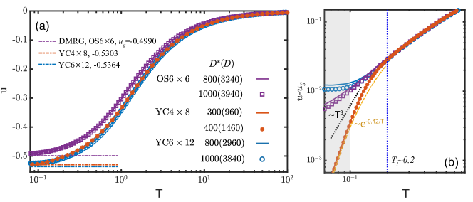
In Fig. S8, we analyze the internal energy per site, $u(T)\equiv\tfrac{1}{N}\langle H\rangle_{T}$ with $c_{V}(T)\equiv\tfrac{\partial u}{\partial T}=-\beta\tfrac{\partial u}{\partial\ln\beta}$ Chen et al. (2018), versus temperature and compare it to the ground state DMRG results on the same geometry. We show data for various geometries, including the YC$6\times 12$, OS$6\times 6$, and small YC$4\times 8$ lattices. It can be observed that the energy data are well converged with bond dimension $D^{\ast}=1000$ (for YC6 and OS6) and $D^{\ast}=400$ (YC4), which correspond to nearly $D\sim 4\times D^{\ast}$ in terms of $U(1)$ states (see legend).

At low temperature, the $u(T)$ curves already closely approach the zero-temperature limits $u_{g}$ [horizontal markers Fig. S8(a)] obtained by ground state density matrix renormalization group (DMRG) calculations. For a strong comparison, we replot the same XTRG data in Fig. S8(b), but now relative to the DMRG ground state energy $u_{g}$ on a log-log plot. The data for the intermediate to large temperature regime, $T>T_{l}$, scales similarly for all boundary conditions (with minor offsets due boundaries). As $T$ decreases below $T_{l}$, the YC4 data converges exponentially, in agreement with the stripe-phase scenario revealed in Ref. Chen et al. (2018). In contrast, the OS6 and YC6 data collapse onto each other down to temperatures well below $T_{l}$ (here the upturn in the YC6 system (blue data) is attributed to finite-$D$ accuracy). Note that from the OS6 data in Fig. S8(b), one may estimate an approximate power-law behavior.

II.4 System size dependence of low-temperature scale $T_{l}$

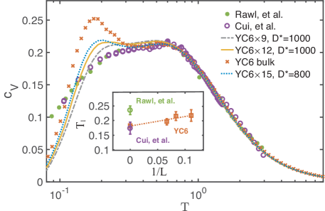
In Fig. S9 we provide the scaling of the lower characteristic temperature $T_{l}$ vs. length $L$ for various YC6 lattices. As $L$ increases, the lower peak/shoulder structure only slightly shifts towards lower temperatures, while it also becomes more pronounced, suggesting stronger 120^∘ correlations in the system [in accordance with $S(K)$ data in Fig. 3(e) in the main text].

In the inset of Fig. S9 we plot the estimated position for $T_{l}$ vs. $1/L$, and also indicate the position of shoulder-like structure in experimental curves Cui et al. (2018). Note that there exists some arbitrariness in determining $T_{l}$ from peak/shoulder structure, as reflected in the error bars. Furthermore, in order to reduce the finite-length effect in YC6 data, we take the difference between YC$6\times 12$ and YC$6\times 9$ data (divided by the $6\times 3$ extra sites) as a YC6 “bulk” results, whose lower peak is even more pronounced and the corresponding $T_{l}$ well agrees with experiments, up to error bars.

Figure S9: Specific heat on YC6 for three different lengths, also compared to experimental data. The ‘YC6 bulk’ is obtained by subtracting YC$6{\times}9$ from YC$6{\times}12$ data, in order reduce the effects from the open boundary. The inset shows the lower characteristic temperature $T_{l}$ vs. $1/$L with estimated error bars from the determination of $T_{l}$ for the peak/shoulder structure. The data point at $1/L=0$ is taken from ‘YC6 bulk’ curve which, indeed, approximately represents an extrapolation in $1/L\to 0$, as suggested by the dotted line. In particular, to determine $T_{l}$ in experimental curves, we assume the shoulder is sitting on top of an approximately linear slope of the $T_{h}$ peak: take $T_{l}$ as the temperature where the curvature of $c_{V}(T)$ is maximally negative (i.e., the local minimum of the curvature around the shoulder). Note the sparse experimental data has been interpolated by $4$th to $6$th order polynomial fittings.

Figure S10: Correlation length, $\xi$, on various YC cylinders, together with HTSE-2D data Elstner et al. (1993) for comparison. For reference, we also added the exponential increase $\xi\propto T^{-1/2}e^{T_{l}/2T}$ predicted by field-theoretical arguments (red dotted line) Chakravarty et al. (1988).

II.5 Correlation length vs. temperatures

Assuming the Ornstein-Zernicke form of the static structure factor $S(q)=S(q_{0})/[1+\xi^{2}(q-q_{0})^{2}]$, in the close vicinity of the ordering momentum $q_{0}$, this defines the correlation length Elstner et al. (1993, 1994) as

$$\xi^{2}\cong\left.\tfrac{1}{2S(q)}\tfrac{\partial^{2}S(q)}{\partial q^{2}}\right|_{q=q_{0}}=\tfrac{c^{2}_{q_{0}}}{2S(q_{0})}\sum_{j}r_{0j}^{2}\,e^{-iq_{0}\cdot r_{0j}}\,\langle\bm{S}_{0}\cdot\bm{S}_{j}\rangle\text{ ,}$$ (S12)

where $r_{0j}\equiv r_{j}-r_{0}$ with $r_{j}$ the lattice location of site $j$, with $j$ running over the whole lattice, and again $r_{0}$ fixed in the center of the system. The constant $c^{2}_{q_{0}}\equiv\langle\cos^{2}\alpha_{0j}\rangle\in[0,1]$ accounts for an angular average with $\alpha_{0j}$ the angle in between $q_{0}$ and $r_{0j}$. In the present context of the TLH, we chose $q_{0}=K$ as the ordering momentum which leads to $c^{2}_{0}=1/2$.

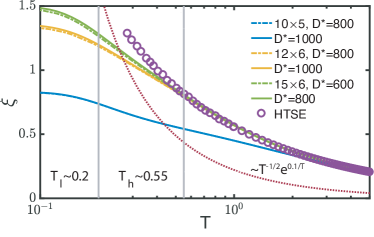
From Fig. S10, one observes that the correlation length $\xi$ remains very short, in that it is below one lattice spacing down to temperatures even below $T_{h}\sim 0.55$ also for the wider systems, in agreement with HTSE-2D in the thermodynamic limit. At lower temperatures, the correlation length gets enhanced with increasing width $W$ and length $L$. Given the very short correlation length of just a very few lattice spacings for $T_{l}<T<T_{h}$, incipient order can be ruled out in this intermediate regime. Instead, we associate this regime with activated RLEs (with minima at $M$), which suppresses the long-range order formation at $K$ and thus leads to a short $\xi$. As temperature is lowered further, the correlation length $\xi$ is expected to increase exponentially. As for our XTRG data, $\xi$ keeps increasing down to $T\sim 0.1$, where it saturates due to the finite system size.

II.6 Entanglement spectra vs. temperatures

Figure S11: (Color online) (a) Entanglement spectrum, $E_{S}$, across a vertical cut in the middle of a YC$6{\times}12$ system versus temperature $T$, where the color differentiates the SU(2) spin symmetry sectors as indicated in the legend. Two temperature scales $T_{l}\sim 0.2$ and $T_{h}\sim 0.55$ are indicated with the grey dashed lines. (b) The same $E_{S}$ data, yet scaled by $\ln{(1+T/a)}$ with $a\sim T_{l}$. With this the high temperature spectra in (a) with $E_{S}\sim\ln T$ Chen et al. (2018) become horizontal lines. At low $T<T_{l}$, empirically, the chosen scale factor $1/\ln(1+\tfrac{T}{T_{l}})\sim 1/T$ still represents a sensible scaling for the lowest levels, thus suggesting $E_{S}\sim T$ there.

Figure S12: (Color online) Entanglement spectrum ($E_{S}$) of entanglement Hamiltonian $\mathcal{H}_{\mathrm{ES}}$ with SU(2) spin quantum number $S$ at (a) $T=0.05$, (b) $T=0.19\simeq T_{l}$, and (c) $T=0.53\simeq T_{h}$. The dashed lines are guide for eyes, indicating the increasing slopes of the “towers” with increasing temperatures. (c) Counting the number of states $\mathcal{N}(E_{S}\leq E_{r})$ for $E_{r}=3,4,5,10$, at various temperatures. It is observed that $\mathcal{N}$ increases as $T$ decreases, and for a range of intermediate energies, say, $E_{r}=4,5$, $\mathcal{N}$ scales approximately polynomially vs. $T$ for $T<T_{l}$, with $\sim T^{-0.44}$ (see text) shown as guid to the eye.

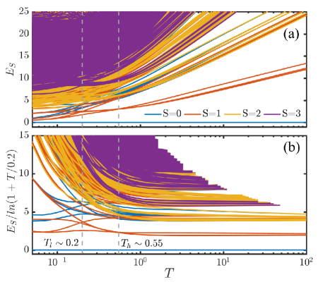
In Fig. S11, we analyze the “renormalization-group” flow of the MPO entanglement spectra of the thermal state, $\rho(\beta)$ vs. the logarithm of the energy scale $T$, for a vertical cut across the middle of a YC$6{\times}12$ system, with focus on the two temperature scales $T_{l}$ and $T_{h}$. This is significantly more detailed than the single number in terms of the MPO entanglement entropy $S_{E}$, e.g., as analyzed in Fig. 3(f) in the main paper. The entanglement spectra are also derived from the normalized ‘purified’ thermal state $|\rho(\beta)\rangle$ and its reduced density matrix $\mathcal{R}(\beta)_{I,I^{\prime}}\equiv\sum_{J}|\rho_{I,J}\rangle\langle\rho_{I^{\prime},J}|$ Chen et al. (2018), where $I,J$ represent degrees of freedom in left and right half of the system, respectively, and $\beta$ is the inverse temperature. Then, the entanglement spectrum, $\tilde{E}_{S}$, at a given inverse temperature, $\beta$, is obtained by diagonalizing $\mathcal{H}_{\mathrm{ES}}\equiv-\ln{\mathcal{R}}$. These are analyzed relative to their ‘ground-state energy’, i.e., $E_{S}\equiv\tilde{E}_{S}-E_{0}$.

In the entanglement spectra $E_{S}$ in Fig. S11, the different symmetry sectors of the MPO virtual bond states are differentiated by color as indicated in the legend. We show eigenstates for each spin symmetry sector, up to a largest ‘energy’ $E_{S}\leq 25$, which corresponds to a weight in the density matrix as low as $\geq e^{-25}\sim 10^{-11}$. From Fig. S11, we can see that, while in the high temperature regime the levels in $E_{S}$ are rather far apart (i.e. the MPO is close to a product state), they become much more dense with decreasing temperature. They show systematic qualitative changes, and in particular line-crossings in the ‘low-energy sector’ around $T_{l}$ and $T_{h}$. For $T<T_{l}$, the entanglement spectra show a systematic (algebraic) approach towards the ‘ground state’, with Fig. S11(b) roughly suggesting $E_{S}\sim T$ for the lowest levels once $T<T_{l}$. These distinct behaviors of $E_{S}$ in different temperature regimes are consistent with the existence of two temperature scales.

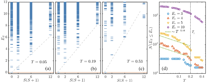
In Fig. S12(a-b), we study the spectroscopy of the entanglement Hamiltonian $\mathcal{H}_{\mathrm{ES}}$. The entanglement levels are plotted with respect to different symmetry labels from $S=0$ up to $S=4$, at $T=0.19$ and $0.05$, respectively. As indicated by the gray dashed lines, the lowest level in each symmetry sector decreases, roughly algebraically as we cool down the system, while also the slope systematically decreases. As a consequence, the number of states with weights $E_{S}<E_{r}$, denoted by $\mathcal{N}(E_{S}\leq E_{r})$, increases as $T$ decreases. We plot $\mathcal{N}(E_{S}\leq E_{r})$ in Fig. S12(d) with $E_{r}=3,4,5,10$. From this we observe that $\mathcal{N}(E_{S}\leq E_{r})$ increases roughly polynomially when $T\leq T_{l}$, indicated by the green dashed lines. If furthermore, we assume rather heuristically that for intermediate $E_{r}$, say, $E_{r}=4$ or 5, each level in the range $E_{S}\leq E_{r}$ contributes crudely equally to the thermal entropy $S_{E}$ of the entanglement Hamiltonian $\mathcal{H}_{ES}$ system, this is consistent with an expected log-scaling of the entanglement entropy, $S_{E}\sim\ln{\mathcal{N}}\propto a_{\mathcal{N}}\ln{\beta}+b$. And, indeed, this hand-waving argument agrees with the scaling $S_{E}\propto a\ln{\beta}+b$ for $T\leq T_{l}$, as observed and discussed with Fig. 3(f) in the main text, even with roughly consistent slope $a_{\mathcal{N}}\approx a=0.44$, also shown in Fig. S12(d) as guide to the eye.

II.7 Spin wave analysis

Figure S13: (Color online) Low-temperature specific heat $c_{V}$ from the spin wave analysis, with and without $1/S$ corrections Starykh et al. (2006), where the gray dashed line indicates the $T^{2}$ behaviors of $c_{V}$ at low $T$ due to the linear spin wave dispersion $E_{k}\propto k$ for small $k$. Inset shows the difference between the two approximations. The vertical markers indicate the two energy scales $T_{l}$ and $T_{h}$ as specified.

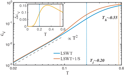
Linear spin wave theory (LSWT) can very well capture the $120^{\circ}$ order in the ground state of TLH Jolicoeur and Le Guillou (1989); Chubukov et al. (1994); Chernyshev and Zhitomirsky (2009). It is thus also believed that LSWT is able to describe thermodynamics at very low temperatures. Here we take the spin wave spectra with and without $1/S$ corrections [Eq. (12) from Starykh et al. (2006)], compute the specific heat according to the conventional Bose-Einstein distribution of magnon gas, and draw a comparison to our two-temperature-scale scenario.

In Fig. S13, we can see that the $c_{V}$ curve with $1/S$ corrections also exhibit a “shoulder-like” structure at around $T_{l}$, below which it gradually changes into a $T^{2}$ scaling, coinciding there with pure LSWT results at low $T$.

The $1/S$ correction gives rise to the difference $\Delta c_{V}$ which, as manifested in the inset of Fig. S13, strongly affects the intermediate temperature regime in between $T_{l}$ and $T_{h}$. $\Delta c_{V}$ starts to decrease rapidly below $T\sim T_{l}$, and the influences of RLEs as well as other renormalization effects in the spectrum due to $1/S$ corrections are largely absent below $T=0.1$. This is consistent with our spin structure factor as discussed with Fig. 3(c-e), where $S_{M}$, representing the activation of RLEs, also becomes clearly weakened below $T_{l}$.

The LSWT analysis of $c_{V}$ and its $1/S$ correction in Fig. S13 thus further confirms the existence of two temperature scales, and, in particular, the lower one $T_{l}$. Overall, Fig. S13 provides useful complementary thermal data to our finite-size XTRG results.

II.8 Chiral Correlations on YC4

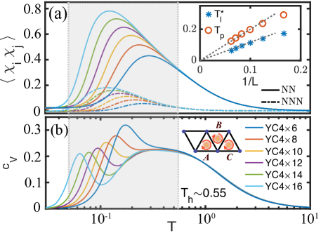
This section complements the analysis of chiral correlations in Fig. 5 in the main paper, in that we focus on the case of YC4 which is special, in that $T_{l}^{\ast}$ scales to zero as $L\to\infty$ (hence the asterisk with $T_{l}$). From Fig. S14 we observe that short-ranged (NN and NNN) chiral correlations build up and become strong at intermediate temperatures, $T_{l}^{*}\lesssim T\lesssim T_{h}$. Clearly, the peak at $T_{p}$ in the chiral correlations [Fig. S14(a)] correlates with the low-energy scale $T_{l}^{*}$ derived from $c_{V}$ [Fig. S14(b)]. Below $T_{l}^{*}$, chiral correlations become negligibly small, which is also directly confirmed by DMRG simulations (not shown). While YC4 also enters an anomalous liquid-like regime for $T<T_{h}$, it becomes a stripe phase below a low-energy scale $T_{l}^{*}$ which diminishes to zero in the thermodynamic limit as demonstrated in the inset to Fig. S14(a) Chen et al. (2018). This is qualitatively different from $T_{l}\sim 0.20$ in wider cylinders and strips, where it becomes a stable temperature scale vs. various system sizes and boundary conditions as shown and discussed with Fig. 2(a). Importantly, Fig. S14 demonstrates that the peak $T_{p}$ in the chiral correlations closely follows the low-energy scale $T_{l}$ derived from the specific heat. In this sense we conclude that they can be ascribed to the same crossover scale that separates the low-energy (here stripe) order from the intermediate regime and, moreover, that finite chiral correlations constitute a characteristic property of the intermediate regime.

Figure S14: (Color online) (a) Chiral correlations compared to (b) specific heat $c_{V}$ in YC4 for various lengths $L$. In (a) we consider correlations between nearest- (NN) and next-nearest neighboring (NNN) triangles in the system center [i.e., using $i=A$ and $j=B,C$ as shown in the inset of (b) with the triangles taken in the system center [cf. Fig. 1]. The disappearance of the low-energy regime for $1/L\to 0$ is specific to YC4 Chen et al. (2018). The inset shows finite size scaling of the peak position, $T_{p}$, in the chiral correlations $\langle\chi_{i}\chi_{j}\rangle$, as well as of the temperature scale, $T_{l}^{*}$, derived from the lower-temperature peak in $c_{V}$ from (b).

Figure S15: (Color online) (a) Specific heat, as well as thermal entropy (inset), of $J_{1}$-$J_{2}$ TLH, with $J_{2}=-0.05$, $0$, and $0.05$, on YC$6\times 9$ geometry. (b,c,d) show the structure factors at $T\simeq 0.53$ near the high temperature scale $T_{h}$.

III Tune spin frustration by deforming the triangular-lattice Heisenberg model

III.1 $J_{1}$-$J_{2}$ Triangular lattice Heisenberg model

To shed further light on the two-temperature-scale scenario, we deform the TLH by including a small but finite next-nearest coupling $J_{2}$,

$$H=J_{1}\sum_{\langle i,j\rangle}\vec{S}_{i}\vec{S}_{j}+J_{2}\sum_{\langle\langle i,j\rangle\rangle}\vec{S}_{i}\vec{S}_{j},$$ (S13)

having $J_{1}\equiv J=1$. A small AF coupling $J_{2}>0$ adds frustration, and hence suppresses 120^∘ ordering on a three-sublattice configuration Zhu and White (2015); Hu et al. (2015); Iqbal et al. (2016); Gong et al. (2017), while $J_{2}<0$ reinforces the ferromagnetic correlations between two spins on the same $120^{\circ}$ sublattice.

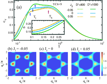
In Fig. S15 we compare the specific heat $c_{V}$ of YC$6\times 9$, for $J_{2}=0$ with $J_{2}=\pm 0.05$. From the temperature dependence in Fig. S15(a) we can see that as we change $J_{2}$ from $-0.05$ to $0.05$, the $T_{l}$ peak systematically shifts to lower temperatures, while at the same time, it weakens. In contrast, the broad peak at $T_{h}$ keeps its position while varying $J_{2}$. The overall downward shift for temperatures $T\gtrsim 0.2$ and upward shift for very small temperatures suggests that with increasing $J_{2}$, more entropy is transferred to lower temperatures. Indeed, as shown in the inset of Fig. S15(a), compared to $J_{2}=0$ case, thermal entropy $S$ at $T=0.1$ is increased (decreased) by $\sim 15\%$, when $J_{2}=0.05$ ($-0.05$) is introduced.

The sensitivity of the structure factor on $J_{2}$ is analyzed in Figs. S15(b-d). As expected, increasing $J_{2}$ significantly reduces the weight $S(K)$, but enhances the weight $S(M)$. This is consistent with dynamical calculations of the $J_{1}$-$J_{2}$ TLH Ferrari and Becca (2019), as well as that includes spin XXZ anisotropy Ghioldi et al. (2015), which show that RLEs are renormalized downward by increasing $J_{2}>0$, giving rise to an extended dispersive continuum above the “roton” minimum.

Figure S16: (Color online (a) Specific heat data for the frustrated SLH on a $6\times 12$ cylinder with $J_{t}$ varied from 0 to 1, keeping up to $D^{\ast}=500$ multiplets [$1790$-$2010$ U(1) states]. The inset traces the low-temperature peak (or shoulder) in the $c_{V}$ curves. (b) Static structure factor $S(q)$ at $C=(\pi,\pi)$ (lines with markers) and $M=(0,\pi)$ (solid lines). The constant offset towards large $T$ is a trivial finite size effect: it is the same for $S(M)$ and $S(C)$ (note the significantly different vertical scales for $S(C)$ [left axis] and $S(M)$ [right axis]) and comes from the $r_{j}=r_{0}$ contribution in the definition of the structure factor, which gives a constant $\langle\bm{S}^{2}\rangle_{T}=\tfrac{3}{4}$. (c) Thermal entropy $S$ decreases from $\ln 2$ as $T$ is lowered. The thermal entropy moves to larger values as the frustration is turned on via $J_{t}$.

III.2 Frustrated square-lattice antiferromagnet

Besides adding $J_{2}$ in to TLH, we can also deform the Hamiltonian towards the square lattice Heisenberg (SLH) model via a tuning parameter $J_{t}$ where $J_{t}=1$ corresponds to the TLH, and $J_{t}=0$ to the SLH. The corresponding Hamiltonian of the frustrated SLH is given by,

$$H=J\sum_{\langle i,j\rangle}\vec{S}_{i}\cdot\vec{S}_{j}+J_{t}\sum_{\langle\langle i,j\rangle\rangle}\vec{S}_{i}\cdot\vec{S}_{j},$$ (S14)

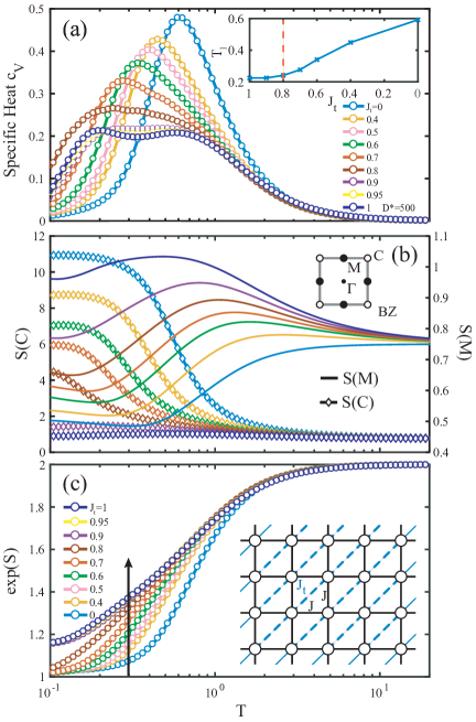
where $\langle.,.\rangle$ denotes nearest-neighbor, and $\langle\langle.,.\rangle\rangle$ next-nearest neighboring pairs of sites along one of the diagonals only [e.g., as depicted in the inset to Fig. S16(c)]. Their respective coupling strengths are given by $J$ and $J_{t}$, where again $J=1$ sets the unit of energy, unless specified otherwise. The system features square lattice Néel order at $T=0$ for $J_{t}=0$, leading to low-$T$ RC behavior Manousakis (1991). Finite $J_{t}>0$ introduces frustration in the system, which leads to an abrupt onset of an incommensurate spiral wave at some critical $J_{t}^{c}\sim 0.79$ Weichselbaum and White (2011). For the isotropic TLH at $J_{t}=1$ this turns commensurate and yields the familiar $120^{\circ}$ order. Our results for the SLH on a $6\times 12$ cylinder (i.e. $L=2W=12$) are summarized in Fig. S16, where we vary $J_{t}$ from $0$ to $1$ (see legend), with $D^{\ast}=500$ multiplets kept.

The specific heat $c_{V}$ is shown in Fig. S16(a). The tracked lowest temperature scale, i.e., global peak position for $J_{t}\leq 0.8$ and the position of the lower shoulder for $J_{t}>0.8$, is plotted as ‘$T_{l}$’ in the inset. This scale starts from about $T_{l}=T_{h}\sim 0.6$ for $J_{t}=0$ (i.e., the pure SLH case). While $T_{l}$ decreases gradually with increasing $J_{t}$, at the same time a shoulder emerges at the original peak position $T_{h}$ which only marginally moves to smaller values. At around $J_{t}\simeq 0.8$, the single peak in the specific heat for small $J_{t}$ is about to fully split into two peaks. There $T_{l}$ has already nearly also reached its final value of $0.2$ for $J_{t}=1$, i.e., the isotropic TLH. Interestingly, the critical value for which ground state calculations observe the onset of incommensurate correlations, $J_{t}^{c}\sim 0.79$ Weichselbaum and White (2011), roughly coincides with the $J_{t}$ for which a well separated two-peak structure has developed at finite $T$ (for the finite size systems here even with a minimum in between), where $T_{l}$ is already also close to its final value of 0.2 for the TLH.

To understand the physical meaning of the temperature scales and their behaviors under various $J_{t}$, we look at the static structure factors, $S(C)$ and $S(M)$, in Fig. S16(b). The points $C$ and $M$ in reciprocal space are pointed out in the inset. We observe that, for $J_{t}\lesssim J_{t}^{c}$, the AF magnetic order [at $C=(\pi,\pi)$, i.e., Néel order] melts most rapidly at the characteristic temperature $T_{l}$. The magnetization per site may also be estimated in the present case by $m\approx\sqrt{S(C)/N}$ (note the slightly different normalization due to angular average as compared to the TLH). For $J_{t}=0$, this yields $m\sim 0.39$ which overestimates the thermodynamic limit $m\sim 0.31$ White and Chernyshev (2007) due to finite-size effects.

The stable large energy scale at $T_{h}$ relates to different physics, here argued to be RLEs. This argument can be solidified by analyzing the structure factor at the point $M=(0,\pi)$ which, indeed, shows anomalous enhancement at intermediate temperatures for finite $J_{t}$. Note that the position of the maximum in $S(M)$ changes from $\sim 1.5$ for $J_{t}=0.6$ to the value of $T_{h}\sim 0.55$ itself for $J_{t}=1$.

In Fig. S16(c), finally, we still present data for the thermal entropy $S$ for various $J_{t}$ values. From this we can see an anomalous enhancement of the entropy as $J_{t}\gtrsim J_{t}^{c}\sim 0.8$. It is remarkable to find the zero temperature commensurate-incommensurate transition also reflected here as a (residual) entropy enhancement in our thermal calculations at our lowest temperatures.

In summary, the specific heat as well as the static structure factor data in Fig. S16 provide further strong support for the emergence of a two-temperature-scale scenario at sufficiently large frustration $J_{t}$, including the $J_{t}=1$ TLH.